Observing braneworld black holes

Abstract:

Spacetime in the vicinity of an event horizon can be probed using observations which explore the dynamics of the accretion disc. Many high energy theories of gravity lead to modifications of the near horizon regime, potentially providing a testing ground for these theories. In this paper, we explore the impact of braneworld gravity on this region by formulating a method of deriving the general behaviour of the as yet unknown braneworld black hole solution. We use simple bounds to constrain the solution close to the horizon.

1 Introduction

Black holes are a fascinating topic of study, whether it be to explore the geometry of strong gravity and its quantum effects, or to understand the astrophysics of massive objects in our galaxy. From the point of view of standard physics in four dimensions, black holes are well described by the Kerr-Newman family of solutions, solutions in standard four-dimensional Einstein-Maxwell gravity. However, the true nature of gravity, though well measured from tabletop to solar system scale experiments, is surprisingly less well determined at larger or smaller scales. For example, the assumptions of dark matter and/or energy are made in order to fit the observed Universe with Einstein theory, yet it is quite possible that it is the theory of gravity which should be altered to fit these data instead.

Theoretically, the possibility that gravity might not be fundamentally four-dimensional, or indeed Einsteinian, is gathering credence. This is in part an impact of superstring theory, which is consistent in ten dimensions (or M-theory in eleven dimensions), but also the more phenomenological recent developments of “braneworld” scenarios, [1, 2], have had a direct influence on studies of more exotic gravitational theories in four-dimensions. Experimentally, the small scale implications of alternative theories of gravity have focused on the impact of Kaluza-Klein (KK) modes or small black holes in colliders, [3, 4], cosmic ray showers, [5], or in particle interactions in supernovae or nucleosynthesis, [6]. Large scale implications of modified gravity have been conducted mostly within the MOND (modified Newtonian gravity) set-up [7], although some preliminary studies have investigated braneworld modifications to the microwave background [8]. Interestingly, while much theoretical work has been done on black holes in modified or higher dimensional gravity theories, there is very little direct link with experimental data so far. Yet there are observations of astrophysical black holes which provide some constraints on strong gravity. Stellar remnant black holes, with masses of about 10 times the mass of our Sun, can form as a result of very massive star evolution. Most stars form in binary systems, so if the companion star is close enough then it can provide a source of material falling onto the black hole. This material has the angular momentum of the orbit so it forms a ring, but angular momentum transport (via a magnetic dynamo process, [9]) spreads this ring out into a disc. The magnetic dynamo also dissipates energy, so this means that there is emitting material down to the last stable orbit around the black hole.

For large mass accretion rates this disc emission takes a rather simple form as the material is optically thick. The energy is emitted and absorbed many times before it escapes the disc, so thermalizes to a blackbody spectrum at a given radius. The total disc spectrum is a sum over all radii of these different temperature blackbodies, with the maximum temperature (which is of order 1 keV for these stellar mass black holes) being set by the emission from close to the inner edge of the disc [10]. The combination of observed disc luminosity and temperature can constrain the size of the inner disc radius, while dynamical studies of the orbit can constrain the black hole mass. Together these give an estimate of the innermost stable orbit in terms of Schwarzschild radii. Current observations indicate that this is generally of order $6GM$, as expected for a Schwarzschild black hole, though there are a few objects with significantly smaller radii, which are interpreted as moderate spin Kerr black holes [11].

Another observational tracer of the gravitational field comes from a corona above the disc, which forms a high energy tail to the disc emission. These high energy X-rays illuminate the disc and form an iron fluorescence line, produced from material with a large rotational velocity in a strong gravitational field. Thus what is seen at infinity is affected by both special (doppler shift, length contraction, time dilation) and general (gravitational redshift) relativistic effects. Together these transform an initially narrow atomic transition into a broad, skewed and reddened line profile. Current observations indicate that the observed lines are consistent with material close to the last stable orbit in Schwarzschild or Kerr black holes [12]. These relativistic effects also distort the spectrum of the intrinsic (sum of blackbodies) disc emission [13].

Thus black holes provide a promising test bed for testing our understanding of gravity. While stellar, or galactic, black holes do not provide regions of high curvature, at least at the classical level, if we accept as fact that black holes radiate, then it is likely that close to the event horizon quantum effects become relevant. Alternatively, the effect of higher dimensions or additional fields in the gravity sector might begin to make their presence felt as the event horizon is approached. In this paper we explore the case of braneworld black holes.

The braneworld paradigm views our universe as a slice of some higher dimensional spacetime. Unlike the Kaluza-Klein picture of extra dimensions, where we do not notice the extra dimensions because they are so small and our physics is ‘averaged’ over them, the braneworld picture can have large, even non-compact, extra dimensions which are unobservable at low energies since we are confined to the brane. Naturally, at not so low energies, the extra dimensions can have experimental consequences [1, 2]. Confinement to the brane, while at first sounding counter-intuitive, is in fact a common occurrence. The first braneworld scenarios [14] used topological defects to model the braneworld, and zero-modes on the defects to produce confinement. Of course in string theory, D-branes have ‘confined’ gauge theories on their worldvolumes.

The braneworld scenario provides a set-up in which we have standard four-dimensional physics confined to the brane, but gravity (and possibly a small number of other fields) propagating in the bulk. The new phenomenology of braneworld scenarios is then primarily located in the gravitational sector, with a particularly nice possible resolution of the hierarchy problem being its primary motivation. Clearly however, the astrophysical and cosmological implications of such a scenario have a more immediate, and more directly measurable, impact. For these issues, the most popular model to explore, and the one which we will be using, has been the Randall-Sundrum scenario, [2], which consists of a domain wall universe living in five-dimensional anti-de Sitter (adS) spacetime. This model is loosely motivated by the Horava-Witten compactification of M-theory [15].

The Randall-Sundrum model has one (or two) domain walls situated as minimal submanifolds in adS spacetime. In its canonical form, the metric of the braneworld is

$$ds^{2}=e^{-2k|z|}\left[dt^{2}-d{\bf x}^{2}\right]-dz^{2}$$ (1)

Here, the spacetime is constructed so that there are four-dimensional flat slices stacked along the fifth $z$-dimension, which have a $z$-dependent conformal pre-factor known as the warp factor. Since this warp factor has a cusp at $z=0$, this indicates the presence of a domain wall – the braneworld which represents an exactly flat Minkowski universe.

Randall and Sundrum showed in their original papers that although gravity was inherently five-dimensional, and the spacetime was strongly warped, as far as a four-dimensional braneworld observer was concerned, the Newtonian potential of a particle on the brane was indeed the four-dimensional $1/r$ potential. These early results were backed up by more complete analyses confirming that the graviton propagator did indeed have the correct tensor structure, and that the effect of the KK modes was to introduce a $1/r^{3}$ correction to the gravitational potential [16].

Of course, of real interest in astrophysics and cosmology is not the perturbative study of the graviton propagator, but a concrete understanding of the true nonperturbative nature of gravity on the brane. This is what is relevant for a black hole. To some extent, this was provided by the brane-based approach of Shiromizu et. al. (SMS) [17], who used a Gauss-Codazzi approach to obtain the braneworld gravitational equations:

$$G_{\mu\nu}=\Lambda_{4}g_{\mu\nu}+8\pi G_{N}T_{\mu\nu}+\kappa^{2}S_{\mu\nu}+{\cal E}_{\mu\nu}$$ (2)

Here, $\Lambda_{4}$ is a residual cosmological constant on the brane. It represents the mismatch between the brane tension and the bulk negative cosmological constant. (In the RS scenario, the brane tension was precisely tuned to balance out the negative bulk cosmological constant.) The final two terms are the brane gravity effects. The first, $S_{\mu\nu}$, consists of squares of the energy-momentum tensor, which is only relevant at high energies. The final term, ${\cal E}_{\mu\nu}$, is a so-called Weyl term, and consists of the projection of the bulk Weyl tensor onto the brane. Although the SMS equations do provide an apparent nonperturbative description of gravity on the brane, it is important to emphasize that the Weyl term is not given in terms of data on the brane, and is a complete unknown from the brane point of view. Therefore, in order to take a pure brane-based approach to gravity, some assumptions must be made about ${\cal E}_{\mu\nu}$.

Two main nonperturbative gravitational problems are of clear interest: Cosmology, and Black Holes. The first problem, that of finding the braneworld generalization of the FRW universe, has been well explored and understood. Brane-based work concentrates mostly on an explanation of the “non-conventional” energy momentum squared terms, as well as the unknown dark radiation effect from the Weyl term [18]. For cosmology however, the high degree of symmetry present renders the full five-dimensional problem fully integrable [19], and the general cosmological braneworld is fully understood in terms of a slice of a five-dimensional adS black hole [20]. The mass of this bulk black hole then generates the radiation-style Weyl term. It is therefore fair to say that while all the implications may not have been calculated, brane cosmology for the pure RS scenario is pretty well understood.

The situation for the black hole on the brane is somewhat different however. Though it would appear that the two cases are similar in that cosmological branes have a dependence on time as well as the bulk $z$-coordinate, and black holes on radius and bulk $z$-coordinate, in fact, the symmetry groups of the spacetimes are crucially different. For cosmology, the metric splits into two parts – the two dimensions on which it depends, and the spatial part of the universe, which has constant curvature. The mathematics of the cosmological braneworld is therefore a two dimensional field theory which turns out to be totally integrable. For the black hole however, the metric splits into three parts – the two dimensions on which it depends, the time coordinate and the remaining spatial part in which the horizon resides. Thus there are two fields in our two dimensional theory, one of which acquires a potential, and there is no longer a simple solution [21].

The case of the black hole in this braneworld picture now becomes of great interest and importance. Of interest as a problem in higher dimensional gravity, and of importance because the adS/CFT correspondence, [22], relates the classical five-dimensional braneworld black hole solution to the four-dimensional quantum radiating black hole[23, 24]. The first attempt, [25], to find a black hole solution replaced the Minkowski metric in (1) by the Schwarzschild metric, thus creating a black string sticking out of the brane. Unfortunately, as suspected by the authors, this string is unstable to classical linear perturbations [26]. Chamblin et. al. realised that the true localised black hole would be a slice of a five-dimensional accelerating black hole metric (known as the C-metric, [27], in four dimensions), however no such metric has as yet been found. A lower dimensional version of a black hole living on a $2+1$-dimensional braneworld was however presented by Emparan, Horowitz and Myers [28], using this four-dimensional C-metric. Since then, several authors have attempted to find the full metric – notably numerical work by Wiseman [29], and others [30].

In this paper, we are interested in near horizon modifications to General Relativity, which in the absence of a full five-dimensional solution might seem problematic. However, our aim here is not to attempt to answer the full five-dimensional problem, but to revisit the four-dimensional braneworld and to take a practical approach to finding the braneworld metric. The motivation will be to see if we can categorize (preferably analytically) various classes of near horizon behaviour, and to see if there is any universality to the four-dimensional braneworld solutions.

The literature has several special solutions, notably the tidal Reissner-Nordstrom solution of Dadhich et. al. [31], but also the PPN parametrized solutions of Casadio et. al. [32]. Visser and Wiltshire [33] presented a more general method which generated an exact solution for a given radial metric form. All of these approaches however have in common the assumption of an “area gauge” for the radial coordinate, $r$, in the metric, i.e., that the area of the 2-spheres surrounding the black hole behaves as ${\cal A}(r)=4\pi r^{2}$. Thus the area of spheres surrounding the black hole increases monotonically between the horizon and spacelike infinity. However, the monotonicity of ${\cal A}(r)$ is only guaranteed if the dominant energy condition holds, and there is no reason to suppose that this will be the case for the Weyl term, indeed, Dadhich et.  al.  have ${\cal E}_{00}<0$ – a violation of the weak energy condition! In fact, energy conditions are persistently violated in dimensionally reduced theories of gravity.

Our reason for suspecting that ${\cal A}(r)$ is not monotonic lies in the putative higher dimensional C-metric, which would consist of an accelerating black hole being ‘pulled’ by a string. The appropriate higher dimensional metric for a Poincaré invariant string has a turning point in the area function, and the ‘horizon’ is in fact singular [34]. It is therefore possible that this renders the black hole horizon also singular. Moreover, using the dual description of a CFT with cutoff living on the brane [23], a static quantum black hole must have a singular horizon [24]. Since the singularity of the string has a diverging area function, it seems likely that the black hole itself might. Such a turning point in the area function can be thought of as a wormhole in the geometry, so called because the spatial part of the Schwarzschild metric:

$$|ds^{2}|=\left(1-{2GM\over r}\right)^{-1}dr^{2}+r^{2}d\Omega^{2}_{I\!I}={({\tilde{r}}+GM/2)^{4}\over{\tilde{r}}^{4}}d{\tilde{r}}^{2}+{({\tilde{r}}+GM/2)^{4}\over{\tilde{r}}^{2}}d\Omega^{2}_{I\!I}$$ (3)

(where $r=({\tilde{r}}+GM/2)^{2}/{\tilde{r}}$) has this property of the area of spheres decreasing as we approach $r=2GM$, then stationary at $r=2GM$, then increasing again as we move onto the other asymptotically flat régime of the maximally extended Schwarzschild solution. As we will see, this is a very good analogy, as there is an exact analytic braneworld metric which has this spatial form, and simply moves the event horizon relative to Schwarzschild either outside $r=2GM$ or through the wormhole neck onto the other Kruskal branch.

In identifying general features of braneworld solutions, the questions we explore in this paper are:

$\bullet$ When is the horizon singular?

$\bullet$ When does the area function have a turning point?

$\bullet$ When are black hole solutions asymptotically flat?

Within the context of an equation of state of the Weyl term we are able to give definitive answers to all of these questions.

The layout of the paper is as follows. In the next section we derive the braneworld equations in a general gauge and show how to reduce these to a two-dimensional dynamical system for a given equation of state. At this point we give the analytic solution corresponding to the Schwarzschild wormhole. In section 3 we analyze this system in general, showing how to answer the questions above. In section 4 we make contact with the asymptotic linearized propagator, and work on small black holes, and present arguments leading to an analytic near horizon metric. Finally, in section 5, we use this metric to explore the phenomenology of astrophysical black holes.

2 Spherically symmetric braneworld metrics

We start by looking at the general static, spherically symmetric metric on the braneworld. By taking the metric to be static, we are taking the point of view that there exists a five-dimensional solution analogous to the C-metric in four-dimensions which has a timelike Killing vector, and can therefore be ‘sliced’ by the braneworld in such a way as to create a static four-dimensional black hole on the brane. In this we assume that the three-dimensional braneworld black hole constructed from the four-dimensional C-metric has a direct analog in one dimension higher. We note that this produces a static braneworld black hole, and precludes the possibility of a dynamical back-reaction to Hawking radiation, instead corresponding to a Boulware choice of boundary conditions, [24], which give a singular ‘horizon’. It should be noted that there is not a consensus as to whether the braneworld black hole should be static (and therefore singular, by the reasoning of [24]), or time dependent, corresponding to an evaporating black hole, as explored by Tanaka [35].

2.1 The metric

The general static spherically symmetric metric on the brane can be written as:

$$ds^{2}=A^{2}(r)dt^{2}-B^{2}(r)dr^{2}-C^{2}(r)d\Omega_{I\!I}^{2}$$ (4)

Clearly this is not in the simplest gauge, as we can still choose our radial function, $r$, quite arbitrarily, however, it proves to be convenient to use this over-general form in order to choose the best gauge for problem solving, and to compare this to more familiar gauges more readily. The main reason for using this form of the metric, with an arbitrary function for the area of the 2-spheres rather than $r^{2}$, is that there is good reason to believe that the area function might not be monotonic. With this form of the metric, the second derivative of the area radius, $C$, (i.e., the radial function defined by $\sqrt{{\cal A}/4\pi}$) is given by the following combination of the Einstein tensor:

$${C^{\prime\prime}\over C}=-{B^{2}\over 2}\left[G^{t}_{t}-G^{r}_{r}\right]+{C^{\prime}\over C}\left({B^{\prime}\over B}+{A^{\prime}\over A}\right)$$ (5)

therefore, for the area function to be guaranteed to be monotonic, we must have $G^{t}_{t}-G^{r}_{r}\geq 0$, which is equivalent to the dominant energy condition. In usual Einstein gravity this is generally the case, but when there are extra dimensions, or extra fields, this is no longer the case. For example, in the cosmic $p$-brane, [34] the area function actually blows up on the ‘horizon’. Since the cosmic $p$-brane might be expected to have some connection to the higher dimensional C-metric, possibly rendering the ‘horizon’ singular, it is vital that in any exploration of braneworld black holes we do not make the restrictive ansatz of $C=r$.

The ‘vacuum’ brane equations from (2) are

$$G_{\mu\nu}={\cal E}_{\mu\nu}$$ (6)

We follow Maartens [36] in using the symmetry of the physical set-up to put the Weyl energy into the form:

$${\cal E}_{\mu\nu}={\cal U}\left(u_{\mu}u_{\nu}-{\textstyle{1\over 3}}h_{\mu\nu}\right)+\Pi\left(r_{\mu}r_{\nu}+{\textstyle{1\over 3}}h_{\mu\nu}\right)$$ (7)

where $u^{\mu}$ is a unit time vector, and $r^{\mu}$ a unit radial vector. Note that the Weyl energy is in ‘Planck’ units, i.e., there is no preceding $8\pi G$ since ${\cal E}$ is derived from gravitation in the bulk. If we want to compare with 4D matter, we should rescale by $1/8\pi G$.

We now have the equations of motion:

$$G^{t}_{t} = {1\over C^{2}}-{1\over B^{2}}\left[2{C^{\prime\prime}\over C}-2{C^{\prime}B^{\prime}\over CB}+{C^{\prime 2}\over C^{2}}\right]={\cal U}$$ (8)

$$G^{r}_{r} = {1\over C^{2}}-{1\over B^{2}}\left[2{A^{\prime}C^{\prime}\over AC}+{C^{\prime 2}\over C^{2}}\right]=-{({\cal U}+2\Pi)\over 3}$$ (9)

$$G^{\theta}_{\theta} = -{1\over B^{2}}\left[{A^{\prime\prime}\over A}+{C^{\prime\prime}\over C}+{A^{\prime}C^{\prime}\over AC}-{A^{\prime}B^{\prime}\over AB}-{B^{\prime}C^{\prime}\over BC}\right]=-{({\cal U}-\Pi)\over 3}$$ (10)

An alternate and useful equation is the Bianchi identity:

$$\left({\cal U}+2\Pi\right)^{\prime}+2{A^{\prime}\over A}\left(\Pi+2{\cal U}\right)+6\Pi{C^{\prime}\over C}=0$$ (11)

(or conservation of “energy-momentum”).

This system of equations has been solved in many special cases, and more general techniques have also been presented. Briefly, the special cases are the tidal Reissner-Nordstrom solution of Dadhich et. al. [31], or the solutions which assume a given form for the time or radial part of the metric [37]. Visser and Wiltshire [33] presented a more general method which generated an exact solution for a given radial metric form. In all of these cases however, the radial gauge $C=r$ was chosen (although [33] did comment on how to use their method when $C$ was not monotonic).

A reasonable alternative to making guesses for various of the metric functions is instead to follow a pragmatic approach as in cosmology. When solving for an FRW universe, the precise details of the composition of the universe are approximated by an isotropic perfect fluid energy-momentum tensor, and, most pertinently, an equation of state is assumed for this source. Dust ($p=0$) for the later universe, radiation ($p=\rho/3$) for somewhat earlier times, and cosmological constant ($p=-\rho$) for inflation. Clearly the actual evolution and matter content of the universe is more detailed and complicated, but this method is useful, accurate, and universally accepted. Here we propose the analogous approach: an equation of state for ${\cal U}$ and $\Pi$, $\Pi={\gamma-1\over 2}{\cal U}$. Of course, a priori there is no reason to suppose that the Weyl term should obey an equation of state (and indeed we will argue later that it will not) however, it is quite possible that just as the universe is approximately matter dominated or radiation dominated in certain eras, the Weyl term might have certain asymptotic equations of state which may be useful as near-horizon or long range approximations.

2.2 The dynamical system

In the next section we provide a detailed analysis of all equations of state, using the common method of dynamical systems analysis of the equations of motion. In our case, it is clear that the most convenient gauge for this type of analysis is $B=C$. In this case, writing

$$X={C^{\prime}\over C}+2{A^{\prime}\over A}\qquad Y={C^{\prime}\over C}$$ (12)

we have:

$$2X^{\prime}+X^{2}-1 = 3{\cal U}C^{2}={9\over\gamma}(XY-1)$$ (13)

$$1-2Y^{\prime}-Y^{2} = {\cal U}C^{2}={3\over\gamma}(XY-1)$$ (14)

together with the constraint

$$1-XY=-{C^{2}\over 3}({\cal U}+2\Pi)=-\gamma{{\cal U}C^{2}\over 3}$$ (15)

The plot of the $\{X,Y\}$ phase plane gives us curves which are solutions, $X(\rho),Y(\rho)$, to this dynamical system. Whether or not these trajectories correspond to an actual black hole depends on whether the integrated solutions $A(\rho),C(\rho)$ have the behaviour we expect for a black hole, such as an horizon, asymptotic flatness and so on.

It is therefore useful before proceeding with the analysis to extract some asymptotic information from the Einstein equations in order to identify general features of the solution on the phase plane.

2.3 Asymptotic analysis

There are two clear asymptotic regions in which we would like to have some information about the black hole solution - the horizon and infinity. Near the horizon $A\to 0$, and we therefore expect that $X$ will become infinite. Near infinity however we would like spacetime to be asymptotically flat, which means (in the area gauge) $A\sim 1-O(r^{-1})$, $B\sim 1-O(r^{-1})$, $C=r$. Or $A\sim 1-O(e^{-\rho})$, $B=C\sim e^{\rho}+O(1)$ in dynamical system (d.s.) gauge.

For the purpose of clarity, we will look at the far field region in the area gauge, in which the leading behaviour of the Weyl energy and radial metric component is easily read off as:

$${\cal U} = {u_{0}r^{3\over\gamma}\over r^{3}}$$ (16)

$$B^{-2} = 1-{\mu\over r}-{\gamma u_{0}r^{3\over\gamma}\over 3r}$$ (17)

What this clearly shows is that for $0<\gamma<3$ the braneworld metric does not tend to Minkowski spacetime for large $r$. Indeed, even for $\gamma>3$ the metric is not asymptotically flat, since asymptotic flatness requires corrections to Minkowski spacetime to be $O(1/r)$. Therefore, an asymptotically flat braneworld black hole requires an asymptotic equation of state $\gamma<0$.

Near the horizon on the other hand, we cannot assume the area gauge, and integrating the energy conservation equation gives

$${\cal U}\propto A^{-{3\over\gamma}-1}C^{{3\over\gamma}-3}$$ (18)

Whether or not the horizon corresponds to a singularity in the Weyl energy depends on the magnitude and sign of $\gamma$, as well as on the behaviour of $C$.

2.4 A simple analytic solution

We conclude this section by demonstrating the use of both the general gauge $C(r)$, as well as the dynamical system by deriving an alternate form of a known analytic solution with ${\cal U}=0$. A quick glance at the equation of state shows that this is formally the limit $\gamma\to\pm\infty$. Since letting $\gamma$ become infinite decouples the equation of state from the dynamical system, the phase plane is in fact the same whether $\gamma$ is $+\infty$ or $-\infty$. Our main reason for deriving this solution afresh is that we wish to use it in section 5 for a near horizon limit, but clearly, any exact solution is helpful, and our derivation makes the overall structure of the spacetime somewhat clearer than using an area gauge.

For ${\cal U}=0$, (13,14) have the solutions:

$$X,Y=\tanh{(\rho-\rho_{0})\over 2}\ ,\coth{(\rho-\rho_{1})\over 2}$$ (19)

Clearly the former solution is appropriate for $Y$, as this corresponds to

$$C=C_{0}\cosh^{2}{(\rho-\rho_{0})\over 2}$$ (20)

which, since we expect an asymptotically flat spacetime which has $r=e^{\rho}$, gives $C_{0}=4e^{\rho_{0}}$. We then have for $A$:

$$2\ln A+\ln C=2\ln\cosh{(\rho-\rho_{1})\over 2}$$ (21)

or

$$2\ln A+\ln C=2\ln\sinh{(\rho-\rho_{1})\over 2}$$ (22)

i.e.

$$A^{2}A_{0}^{-2}C_{0}\cosh^{2}{(\rho-\rho_{0})\over 2}=\cosh^{2}{(\rho-\rho_{1})\over 2}\ \ {\rm or}\ \ \sinh^{2}{(\rho-\rho_{1})\over 2}$$ (23)

For an horizon, we expect that $A^{2}$ will have a zero, hence we choose the second solution, giving

$$A^{2}={A_{0}^{2}\over C_{0}}\left({\cosh(\rho-\rho_{1})-1\over\cosh(\rho-\rho_{0})+1}\right)$$ (24)

For asymptotic flatness $A_{0}^{2}=4e^{\rho_{1}}$.

Overall the metric is:

$$ds^{2}=e^{\rho_{1}-\rho_{0}}\left({\cosh(\rho-\rho_{1})-1\over\cosh(\rho-\rho_{0})+1}\right)dt^{2}-16e^{2\rho_{0}}\cosh^{4}{(\rho-\rho_{0})\over 2}\left[d\rho^{2}+d\Omega_{I\!I}^{2}\right]$$ (25)

or, writing $r=e^{\rho}$:

$$ds^{2}={(r-r_{1})^{2}\over(r+r_{0})^{2}}dt^{2}-{(r+r_{0})^{4}\over r^{4}}dr^{2}-{(r+r_{0})^{4}\over r^{2}}d\Omega_{I\!I}^{2}$$ (26)

this metric has appeared in the area gauge as [32]

$$ds^{2}=\left[(1+\epsilon)\sqrt{1-{2GM\over R}}-\epsilon\right]^{2}dt^{2}-{dR^{2}\over 1-{2GM\over R}}-R^{2}d\Omega_{I\!I}^{2}$$ (27)

where $R=(r+r_{0})^{2}/r$, $GM=2r_{0}$, and $GM\epsilon=r_{1}-r_{0}$. The anisotropic stress for this solution is $\Pi=3GM\epsilon/AC^{3}$.

Figure 1: Pictorial representation of a constant time slice of the metric (26).

While the area gauge gives a familiar spatial part of the metric, note that at the old Schwarzschild ‘horizon’, $R=2GM$, the $t-t$ component of the metric does not vanish. For $\epsilon>0$, $g_{tt}$ will be zero before $r=2GM$, and the area gauge holds outside the black hole. (Strictly of course, this is not a black hole, as the ‘horizon’ is singular.) If $\epsilon<0$ then $g_{tt}=0$ at $r<2GM$, and $r=2GM$ becomes a coordinate singularity accessible by timelike observers, the result of choosing an inappropriate gauge.

3 The general dynamical system

In order to find a general solution for the braneworld black hole, subject to the proviso that the Weyl energy obeys an equation of state, we will now analyze the general dynamical system:

$$X^{\prime} = {1-X^{2}\over 2}+{9\over 2\gamma}(XY-1)$$ (28)

$$Y^{\prime} = {1-Y^{2}\over 2}+{3\over 2\gamma}(1-XY)$$ (29)

Once again we emphasize that we do not believe that the equation of state will necessarily hold over the whole horizon exterior, simply that it will potentially give various asymptotic behaviours near infinity or near the horizon.

The plot of the $\{X,Y\}$ phase plane gives us curves which are solutions, $X(\rho),Y(\rho)$, to the dynamical system (28,29). These in turn can be integrated to find $A(\rho),C(\rho)$. A selection of representative phase plane plots are given in figure 2.

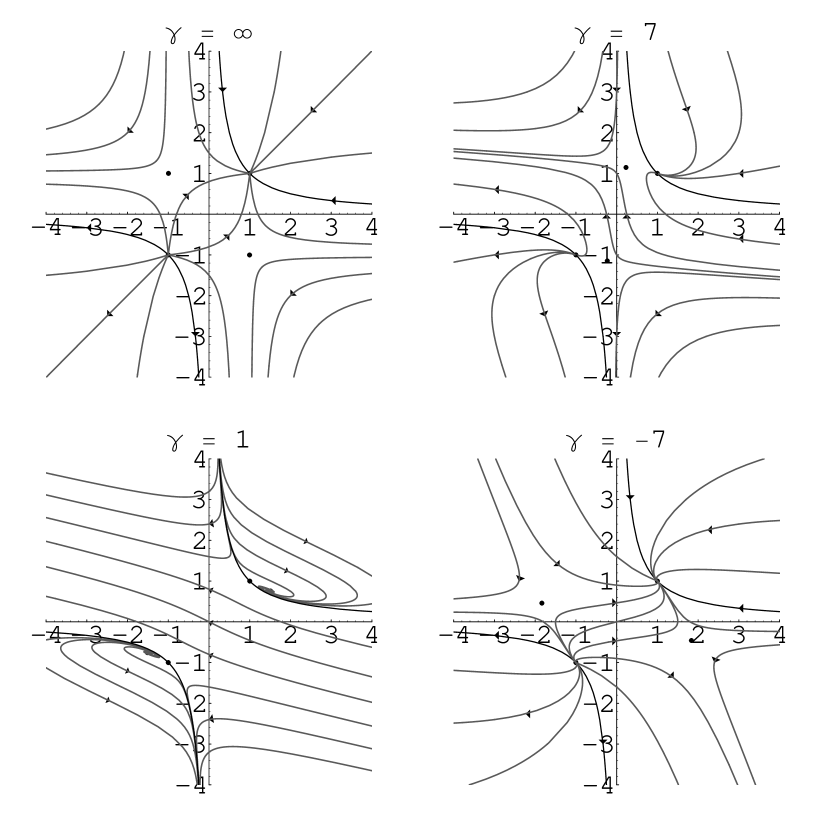
Figure 2: Phase plane for a range of equations of state.

What these plots show is that there are attractors in the phase plane, and that a general trajectory flows in from infinity to one of these attractors. Whether or not these trajectories correspond to an actual black hole depends on whether the integrated solutions $A(\rho),C(\rho)$ have the behaviour we expect for a black hole, such as an horizon, asymptotic flatness and so on.

Briefly, a horizon corresponds to $A\to 0$, therefore we expect $X$ becomes infinite for the black hole horizon. Flat space on the other hand corresponds to $A^{\prime}=0$, $C\propto e^{\rho}$, hence $X=Y=1$. A black hole solution must therefore be a trajectory which comes in from large $X$ (possibly large $Y$ as well) and terminates on $(1,1)$. To find out which equations of state allow this, and whether the area function has any turning points, which correspond to zeros of $Y$, requires a detailed analysis of the phase plane.

3.1 Features of the phase plane

Part of any dynamical systems analysis is an identification and classification of critical points, invariant submanifolds, and other distinguishing features of the phase plane. In this case, the invariant hyperboloid is easily identified from the constraint (15) as $XY=1$. Along this hyperboloid $({\cal U}+2\Pi)=0$, therefore, apart from the special case $\gamma=0$, this corresponds to a vanishing Weyl term, and hence the pure Einstein case – i.e., the Schwarzschild solution. This is given by (20,24) with $\rho_{0}=\rho_{1}$ and $A_{0}^{2}=C_{0}$. If $\gamma=0$, in addition to the Schwarzschild solution we have $X=\pm\sqrt{3}=1/Y$, which is covered by the analysis of the critical points below.

Critical points

The system has 4 critical points ($X^{\prime}=Y^{\prime}=0$):

$$P_{\pm} = \pm(1,1)$$ (30)

$$Q_{\pm} = \pm(27+\gamma^{2})^{-1/2}(9-\gamma,3+\gamma)$$ (31)

The $Q_{\pm}$ critical points move as $\gamma$ runs from $+\infty$ to $-\infty$, from $Q_{\pm}=(\mp 1,\pm 1)$ to $Q_{\pm}=(\pm 1,\mp 1)$. For $\gamma=3$, $P$ and $Q$ are coincident. The nature of the critical points is as follows:

$\bullet$ $3<\gamma$           $P_{+}$ is an attractor and $P_{-}$ a repellor, the $Q$’s are saddle points.

$\bullet$ $0<\gamma<3$    $Q_{+}$ is an attractor and $Q_{-}$ a repellor, the $P$’s are saddle points.

$\bullet$ $\gamma<0$           $P_{+}$ is an attractor and $P_{-}$ a repellor, the $Q$’s are saddle points.

The critical point $(1,1)$ corresponds to flat space:

$$X=Y=1 \Rightarrow A^{\prime}=0,\ C^{\prime}=C$$ (32)

$$\Rightarrow C=e^{\rho}$$

Therefore any asymptotically flat solution must terminate on this critical point. While $P_{+}$ is an attractor, this is not really a problem, but for the range of $\gamma$ where it is a saddle point, only the invariant hyperboloid can satisfy this, and by definition, this is where we have the exact Schwarzschild solution.

The critical point $Q_{+}$ on the other hand, corresponds to a non-asymptotically flat spacetime, which, for $\gamma>-3$ in area gauge is:

$$ds^{2}=r^{2(3-\gamma)\over(3+\gamma)}dt^{2}-{(27+\gamma^{2})\over(3+\gamma)^{2}}dr^{2}-r^{2}d\Omega_{I\!I}^{2}$$ (33)

which we do not expect to be appropriate to the metric for an isolated source. This solution can also be used for $\gamma<-3$, provided one remembers that increasing $r$ actually corresponds to moving towards the black hole ($g_{tt}\to 0$ as $r\to\infty$). This is a genuine wormhole solution, in that the area ${\cal A}(r)$ increases unboundedly towards the event horizon, which is located at infinite proper distance. Unlike the Schwarzschild wormhole however, this inner asymptotic region is not flat, but, as already mentioned, leads in to a null asymptopia. It is perhaps worth noting that the critical value $\gamma=-3$ corresponds to the marginal case of no wormhole, but an infinite throat:

$$ds^{2}=r^{2}dt^{2}-{dr^{2}\over r^{2}}-r_{0}^{2}d\Omega_{I\!I}^{2}$$ (34)

exactly analogous to the extreme Reissner-Nordstrom black hole throat.

The general solution of the braneworld black hole therefore requires $\gamma>3$ or $\gamma<0$ in order to terminate on the critical point $P_{+}$. Luckily, this range of $\gamma$ is precisely that for which spacetime asymptotes flat space, although only for $\gamma<0$ is it actually asymptotically flat.

Asymptotes

Finally, the other region of interest, the black hole horizon, corresponds in general to large values of $X$, for which we can identify the characteristic behaviour.

The line $Y=(\gamma-3)X/(\gamma+9)$ is an asymptote for $\gamma\in[0,3]$, but a separatrix for negative $\gamma$, and $\gamma>3$. It corresponds to the solution

$$ds^{2}=(\rho-\rho_{0})^{24\gamma\over\gamma^{2}+27}dt^{2}-(\rho-\rho_{0})^{4\gamma(\gamma-3)\over\gamma^{2}+27}\left[d\rho^{2}+d\Omega^{2}_{I\!I}\right]$$ (35)

which has a singular horizon.

For negative $\gamma$, and $\gamma>3$ the asymptotic solution is $X=2/(\rho-\rho_{0})$, and $Y\propto(\rho-\rho_{0})^{-3/\gamma}$. This gives the metric

$$ds^{2}=(\rho-\rho_{0})^{2}dt^{2}-C_{0}^{2}\left(1+c_{1}(\rho-\rho_{0})^{1-3/\gamma}\right)\left[d\rho^{2}+d\Omega^{2}_{I\!I}\right]$$ (36)

The horizon is singular in this case for $|\gamma|>3$.

3.2 Special solutions

Because of the number and nature of the critical points, there can be special solutions which start on one critical point and terminate on another. Depending on the value of $\gamma$, the attractor $P_{+}$ can have up to three special solutions corresponding to trajectories from each of the other critical points. It is easiest to demonstrate these solutions for the extreme case $\gamma=\infty$, where we have an analytic solution of the phase plane.

$\bullet$ $P_{-}$ solution:

The solution from $P_{-}$ to $P_{+}$ is easy to define in the analytic case: it is $X=\tanh(\rho-\rho_{1})/2$, $Y=\tanh(\rho-\rho_{0})/2$, which corresponds to a two parameter family solution of metrics:

$$ds^{2}={(r+r_{1})^{2}\over(r+r_{0})^{2}}dt^{2}-{(r+r_{0})^{4}\over r^{4}}dr^{2}-{(r+r_{0})^{4}\over r^{2}}d\Omega^{2}_{I\!I}$$ (37)

For $r_{0}=r_{1}$, this is the Schwarzschild wormhole, and corresponds to the straight line path between $P_{-}$ and $P_{+}$. For $r_{1}\neq r_{0}$, the solution corresponds to the other paths shown in figure 2 between the critical points. The wormhole is supported here by the negative anisotropic stress $\Pi=-6/C^{3}=-6r^{3}/(r+r_{0})^{6}$. See [38] for more detailed discussions of wormhole solutions on braneworlds. Although for finite $\gamma$ the form of this metric will change, the general nature – that of a wormhole connecting two asymptotically flat regions – will not. This solution exists for $\gamma>9$ and $\gamma<-3$.

$\bullet$ $Q_{-}$ solution:

This solution only exists in the $\gamma=\infty$ limit. It has $X\equiv 1$ and $Y=\tanh\rho/2$ which integrates to the metric

$$ds^{2}={r^{2}\over(r+r_{0})^{2}}dt^{2}-{(r+r_{0})^{4}\over r^{4}}dr^{2}-{(r+r_{0})^{4}\over r^{2}}d\Omega^{2}_{I\!I}$$ (38)

which can be seen to be a limiting form of the metric (26) i.e., a wormhole with an inner asymptotic null asymptopia. For $\gamma<-3$, the $Q_{+}$ critical point has $Y<0$ and hence the $Q_{+}\to P_{+}$ solution actually takes this qualitative form.

$\bullet$ $Q_{+}$ solution:

This solution has $Y\equiv 1$ and $X=\tanh\rho/2$ for the analytic form. This integrates to the metric

$$ds^{2}=\left(1+{1\over r}\right)^{2}dt^{2}-dr^{2}-r^{2}d\Omega^{2}_{I\!I}$$ (39)

which is not a wormhole, but a flat 3-space with a distorted Newtonian potential. The solution will have this form for $\gamma>3$, but for $\gamma<-3$, the $Q_{+}$ critical point moves below the $X$-axis, and the solution joining $Q_{+}$ to $P_{+}$ takes the above form (38). For $\gamma=-3$ this trajectory is identical to the extremal Reissner-Nordstrom solution:

$$ds^{2}=\left(1-{r_{0}\over r}\right)^{2}dt^{2}-\left(1-{r_{0}\over r}\right)^{-2}dr^{2}-r^{2}d\Omega^{2}_{I\!I}$$ (40)

In addition, there are special values of $\gamma$ for which there are $Q_{-}\to Q_{+}$ trajectories. Specifically, $\gamma=9$ has a wormhole:

$$ds^{2}={r\over(r+r_{0})^{2}}dt^{2}-{3\over 4}\left({r+r_{0}\over r}\right)^{4}dr^{2}-{(r+r_{0})^{4}\over r^{2}}d\Omega^{2}_{I\!I}$$ (41)

and $\gamma=-3$ has a ‘throat’ solution with bouncing Newtonian potential:

$$ds^{2}=A_{0}^{2}\cosh^{2}r\ dt^{2}-dr^{2}-R_{0}^{2}d\Omega^{2}_{I\!I}$$ (42)

or adS${}_{2}\times S^{2}$.

3.3 Summary

To summarize: the phase plane shows clearly that flat spacetime is a critical point, which is an attractor for equations of state with $\gamma>3$ or $\gamma<0$. Only for this latter range of $\gamma$ is the spacetime asymptotically flat. For these ranges of $\gamma$ the near horizon behaviour is also given by a defined class of metrics (36), which are singular for $|\gamma|>3$. Solutions are allowed both with and without turning points in the area function, though only for $\gamma<-3$ do these correspond to solutions which are asymptotically flat.

In addition, there are special solutions which correspond to trajectories between critical points. The trajectory from $P_{-}$ to $P_{+}$ represents a solution with two asymptotic flat regions, and is a genuine braneworld wormhole. The solution from one $Q$ critical point also represents a wormhole spacetime, which in the case of $\gamma=-3$, has a throat.

4 Physical solutions

In order to decide what a reasonable black hole metric might look like, it is useful to compare to known results, that of the linearized metric, and also the small black hole approximation.

4.1 Comparison with linearized propagator

One region in which we do know the metric of the black hole is at large $r$. Randall and Sundrum, [2], computed the corrections to the Newtonian potential, and Garriga and Tanaka, [16], the correct tensor propagator:

$$g_{tt}=1-{2GM\over{\tilde{r}}}\left(1+{2\over 3}{l^{2}\over{\tilde{r}}^{2}}\right)\hskip 14.22636pt;\hskip 22.76219ptg_{ij}=-1-{2GM\over{\tilde{r}}}\left(1+{1\over 3}{l^{2}\over{\tilde{r}}^{2}}\right)$$ (43)

where we write ${\tilde{r}}$ to distinguish from the $r$-coordinate of the area gauge. Transforming to area gauge gives:

$$g_{tt}=A^{2}=1-{2GM\over r}-{4\over 3}{GMl^{2}\over r^{3}}\hskip 14.22636pt;\hskip 22.76219pt-g_{rr}^{-1}=B^{-2}=1-{2GM\over r}-{2GMl^{2}\over r^{3}}$$ (44)

Substituting into the equations of motion gives an equation of state $\Pi=5{\cal U}/4$, or $\gamma=-3/2$.

Interestingly, this asymptotically flat solution holds down to the event horizon, giving a fully nonsingular solution. The Weyl energy:

$${\cal U}={-4GMl^{2}\over r^{5}}\left(1-{2GM\over r}-{4\over 3}{GMl^{2}\over r^{3}}\right)$$ (45)

has a maximum at $r\simeq 2.4GM$ and returns to zero at the event horizon. This is not the behaviour we would expect from the Weyl energy, hence $\gamma=-3/2$ should be taken only as an asymptotic equation of state.

4.2 Comparison with small black holes

Another common limit used in braneworld black holes is the small black hole limit. Here, if the black hole has mass much less than the adS scale, it is expected that the adS curvature has very little effect on the event horizon, and so the five-dimensional Schwarzschild solution in a good approximation, i.e. $B^{-2}=A^{2}=1-{\mu\over r^{2}}$ in area gauge. A quick check of the asymptotic solution (17) shows that $\gamma=-3$, or $\Pi=-2{\cal U}$. This has ${\cal U}=-\mu/r^{4}$.

A plot of the phase plane for $\gamma=-3$ shows that these

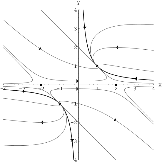
Figure 3: Phase plane for $\gamma=-3$.

trajectories form a stable family of solutions terminating on $P_{+}$. There are no trajectories crossing the $X$-axis as $Y=0$ is a solution to the equations of motion. In other words, there are solutions to the black hole system which represent truly infinite throats with varying Newtonian potentials. For $\gamma<-3$ once again there are trajectories which cross the $Y$-axis, and hence have a bounce in the area function, or a wormhole.

4.3 A possible black hole solution

Having compared the equation of state method with known asymptotic solutions, it is clear that if an equation of state applies, it is generally a negative one. Moreover, from the intuition gained by looking at very small black holes, $\gamma$ curiously becomes more negative closer to the horizon. What sort of equation of state might hold near the event horizon? To explore this, we return to the holographic correspondence.

In string theory, it has been realized for some time that there is a correspondence between string theory on adS space, and a CFT on the boundary of that adS space [22]. In other words, all of the information contained in the five-dimensional gravitational spacetime is encoded in a pure quantum field theory (no gravity) living on a four-dimensional spacetime. In the braneworld picture, the brane is not at the adS boundary, but at a finite distance, and the theory on this brane now contains gravity, as well as a conformal energy-momentum tensor – the Weyl term ${\cal E}_{\mu\nu}$. The effect of the brane on the adS/CFT correspondence therefore is that the bulk theory of gravity in five dimensions corresponds to the four dimensional brane theory of a CFT with a UV cutoff interacting with gravity [23]. Since the brane theory is a quantum theory, the holographic correspondence indicates that the classical bulk solution projects to a quantum corrected solution on the brane [24].

For cosmological solutions, there is a nice holographic interpretation, where the braneworld cosmology can have a radiation source which is the result of the projection of the Weyl curvature of the black hole on the brane. This source can be interpreted as a CFT in a thermal state corresponding to the Hawking temperature of the bulk black hole. The brane cosmological metric has a constant curvature spatial part, and its symmetries demand that only a radiation energy Weyl term is allowed. From the bulk perspective, this means that every point on the brane is at the same distance from the bulk black hole. Thus a flat universe corresponds to a ‘flat’ bulk black hole, a closed universe to a conventional spherical bulk black hole. One way of imagining a braneworld black hole forming is to transport this bulk black hole in towards and onto the brane. In doing this, one breaks this symmetry of equidistance from the black hole. In other words, from the holographically dual brane point of view, we introduce an anisotropic stress by shifting the black hole from its equidistant position. The closer we bring the black hole towards the brane, the more anisotropic the set-up. Therefore, we might expect that $\Pi$ becomes more and more important both as we transport the black hole towards the brane, or as we move closer to the event horizon. Therefore a physically reasonable expectation might be that equations of state with large $\gamma$ are relevant near the horizon.

Taking this reasoning to its logical extreme, we therefore propose as a “working metric” for the near horizon solution the analytic form of section 2.4:

$$ds^{2}={(r-r_{1})^{2}\over(r+r_{0})^{2}}dt^{2}-{(r+r_{0})^{4}\over r^{4}}dr^{2}-{(r+r_{0})^{4}\over r^{2}}d\Omega_{I\!I}^{2}$$ (46)

Clearly, although there is a degree of arbitrariness in this choice, we believe that the horizon is likely to be singular, and also that a turning point in the area function is also likely. This metric has both these features and the added advantage of analyticity, which means that many properties can be calculated explicitly.

5 Testing the solution and future horizons

We now wish to explore some simple tests of the near horizon form (26/46) or (27):

$$ds^{2}=\left[(1+\epsilon)\sqrt{1-{2GM\over R}}-\epsilon\right]^{2}dt^{2}-{dR^{2}\over 1-{2GM\over R}}-R^{2}d\Omega_{I\!I}^{2}$$ (47)

Although this latter form of the metric is not valid throughout the exterior of the horizon if $\epsilon<0$, it is an easier gauge to see the contrasts with the Schwarzschild metric, and since it turns out that there can be no stable orbit within the wormhole region, it is quite satisfactory for working with accretion discs.

The first point to note about (47) is that the ADM and gravitational mass (defined by $g_{tt}$) are no longer the same. Once again, this is quite a common occurance in string gravity, and is a result of the extra degrees of freedom of the gravitational field. As a result, the weak field tests of light bending and perihelion precession will be modified at the $O(\epsilon)$ level, in a way consistent with the PPN formalism.

The near horizon metric (2.24 in area gauge or 4.4 in isotropic coordinates) is very different to the standard Schwarzschild solution. The horizon is always singular even for apparently negligibly small $\epsilon$ (except for $\epsilon=0$ which corresponds to $\cal E{\mu\nu}=0$, so is identically Schwarzschild). This is a true singularity, as the energy density from $\cal E_{\mu\nu}$ becomes infinite at the horizon. An intrepid observer plunging into a supermassive black hole, expecting to sail seamlessly through the horizon and explore spacetime close to the singularity before finally succumbing to tidal forces, is instead crushed out of existence at the horizon. Indeed, they are slammed into the horizon at infinite proper speed! The are no timelike or null geodesics which connect anywhere outside the horizon with the standard Schwarzschild singularity at $r=0$. Infalling matter or light simply cannot reach this point.

Such a drastic change to the spacetime surely has observable effects above the horizon. The metric (4.4) can easily be compared with the PPN formalism, and observational limits on these parameters from solar system tests set limits on $|\epsilon|<10^{-3}$. However, these derive from solar system tests in the weak gravitational field regime. This would only be applicable if the metric (4.4) covered the entire spacetime, but as discussed above we envisage this only as the near horizon asympote of a more general metric. The only mathematical limit on the near horizon metric is $\epsilon>-\frac{1}{2}$ from the requirement that $r_{1}$ is positive definite.

Here instead we constrain $\epsilon$ by connection to the observations of accreting black holes in our galaxy. The luminosity and temperature of the blackbody emission from the accretion disc can be measured from X-ray spectra, giving a direct estimate of the emitting area. There are uncertainties in this approach, but some confidence can be derived from the fact that changes in the luminosity give rise to the $L\propto T^{4}$ behaviour expected from a constant emitting area. Assuming that the uncertainties are less than a factor of 2 then the data strongly constrain the minimum stable orbit to be $<12GM$.

We assume that the ‘near horizon’ metric applies on these size scales and solve the Euler-Lagrange equations from (2.24) in the equatorial plane to find the innermost stable particle orbit, and its associated angular momentum $h=|g_{\phi\phi}|\dot{\phi}$. Table 1 shows these as a function of $\epsilon$, together with the horizon position ($g_{tt}=0$) and the radius at which light can (unstably) orbit around the black hole. We can use the area gauge even for cases where $\epsilon<0$ (which have a wormhole) as the coordinate singularity at $R=2GM$ is below the radii of interest for light and particle orbits. The observations of accretion disc size in X-ray binary systems give an upper limit to $\epsilon$ of about $2$, and are easily consistent with our expectation of $\epsilon<0$. (In the absence of a complete metric from larger to smaller $r$, we have taken $M$ to be the ADM mass.)

$\epsilon$	-0.5	-0.1	0	0.1	0.5	1	2
$R_{h}$	$\infty^{*}$	2.02∗	2	2.01	2.25	2.67	3.6
$R_{ms}$	4.26	5.63	6	6.37	7.88	9.82	13.75
$h^{2}$	4.15	10.11	12	14.03	23.78	39.54	83.06
$R_{ph}$	2.25	2.83	3	3.17	3.91	4.86	6.82

Table 1: Radii for the horizon, $R_{h}$, minimum stable orbit for particles, $R_{ms}$ and the unstable photon orbit $R_{ph}$ in units of $GM$. We also give the associated angular momentum of the minimum stable orbit, $h^{2}$. Note that for negative $\epsilon$, the star indicates that the horizon is on the lower Kruskal branch, and therefore inside R=2GM.

If this asymptotic metric holds to within a few tens of Schwarzschild radii of the horizon then there are potentially observable effects on the spacetime around stellar mass black holes. We will explore these further in a subsequent paper.

Although we have focused on braneworlds, the techniques will clearly be applicable to stringy black holes, or indeed any theory that modifies gravity. In the absence of a concrete solution to test, our approach of trying to find classes of behaviour and some sort of universality near the event horizon seems the best way to proceed. Typically, any covariant theory which modifies the near horizon spacetime structure of the black hole will have these qualitative features, hence similar effects that we have been exploring. All in all, this seems a fruitful alternative to explore in terms of testing ideas in high energy gravity.