hep-th/0406191

RIKEN-TH-27

Large $N$ limit of 2D Yang-Mills Theory and Instanton Counting

Toshihiro Matsuo, So Matsuura and Kazutoshi Ohta

Theoretical Physics Laboratory
The Institute of Physical and Chemical Research (RIKEN)
2-1 Hirosawa, Wako
Saitama 351-0198, JAPAN

Abstract

We examine the two-dimensional $U(N)$ Yang-Mills theory by using the technique of random partitions. We show that the large $N$ limit of the partition function of the 2D Yang-Mills theory on $S^{2}$ reproduces the instanton counting of 4D ${\cal N}=2$ supersymmetric gauge theories introduced by Nekrasov. We also discuss that we can take the “double scaling limit” by fixing the product of the $N$ and cell size in Young diagrams, and the effective action given by Douglas and Kazakov is naturally obtained by taking this limit. We give an interpretation for our result from the view point of the superstring theory by considering a brane configuration that realizes 4D ${\cal N}=2$ supersymmetric gauge theories.

1 Introduction

It has been recently recognized that “duality” is a quite important idea to understand non-perturbative aspects of gauge theories. For example, the duality between gauge theories and string theories [1] is realized as the AdS/CFT correspondence [2, 3, 4] (For review, see [5, 6]), the large $N$ reduction of gauge theories realizes the gauge/matrix correspondence [7, 8, 9, 10] and large $N$ matrix models have been proposed as candidates for non-perturbative definition of the string/M theory [11, 12], and recently, it was found that ${\cal N}=1$ supersymmetric gauge theories closely related to $c=0$ matrix models [13].

Among studies of duality in lower dimensional theories, two-dimensional (2D) Yang-Mills theory has played important roles to examine the nature of the gauge/string correspondence. This theory is exactly solvable [14] and the partition function of 2D $U(N)$ ($SU(N)$) gauge theory on an arbitrary orientable manifold of genus $G$ with area $A$ is exactly given by a sum over all irreducible representations [15];

$$Z_{G}=\sum_{R}(\dim R)^{2-2G}e^{-\frac{\lambda A}{2N}C_{2}(R)},$$ (1.1)

where $\dim R$ and $C_{2}(R)$ are a dimension and quadratic Casimir of the representation $R$. Gross and Taylor have attempted in their seminal works [16, 17, 18] to uncover the relationship between the 2D Yang-Mills theory and a string theory. (For review, see Ref. [19].) Not only the gauge/string correspondence, the equivalence with a $c=0$ matrix model [20] and a $c=1$ matrix model [21] has been studied. As recent developments, a correspondence between the finite $N$ 2D Yang-Mills and a string theory has been discussed [22, 23], and it has been pointed out that 2D Yang-Mills theory relates to 4D black holes [25] and random walks [26].

In this article, we analyze 2D $U(N)$ Yang-Mills theory from the point of view of random partitions and discuss the relation to the instanton counting of 4D ${\cal N}=2$ supersymmetric gauge theories discovered by Nekrasov [27]. The authors of Ref. [27] have used the technique of a summing over random partitions. This technique is powerful enough when partitions or Young diagrams are concerned to carry out the exact calculation of the instanton counting. However, in spite of the beautiful structure of the obtained instanton partition function, the physical meaning of the relationship between the instanton counting and the random partitions is not clear yet.

We show that we can rewrite the partition function (1.1) in the language of random partitions. In particular, we argue that the large $N$ limit of the partition function (1.1) reproduces the instanton counting of a 4D ${\cal N}=2$ supersymmetric gauge theory given in Ref. [28] by a deformation corresponding to the breaking of the gauge symmetry, $U(N)\to U(N_{1})\times\cdots\times U(N_{r})$. We also argue that we can take a “double scaling limit” by fixing the product of $N$ and the size of boxed of Young diagrams, which includes the naive large $N$ limit as a limit of the fixed parameter. We will see that this limit naturally reproduces the discussion by Douglas and Kazakov [20].

This paper is organized as follows. In the next section, we review the definition and some properties of the profile function that is convenient to express partitions. We show that the dimension and the quadratic Casimir of $U(N)$ can be rewritten using the profile function. In the section 3, we take the large $N$ limit of the 2D Yang-Mills theory and show that its partition function gives the instanton counting of a 4D ${\cal N}=2$ supersymmetric gauge theory. In the section 4, we argue the “double scaling limit” of the partition function. In the section 5, we consider a brane configuration which realizes 4D ${\cal N}=2$ supersymmetric gauge theory and 2D Yang-Mills theory, and discuss a string theoretical interpretation for the result that 2D Yang-Mills theory reproduces the instanton counting of the 4D theory. The section 6 is devoted to conclusions and discussions.

2 The profile function of Young diagram

As mentioned in the introduction, the partition function of 2D Yang-Mills theory is given by a sum over all irreducible representations of the gauge group, each of which corresponds to a Young diagram. In this section, we first review the definition and some properties of the “profile function” which expresses the Young diagram systematically, and rewrite the partition function (1.1) using them.

Recalling the one-to-one correspondence between a Young diagram with $k$ boxes and a partition of $k$, $\left\{k_{1},\cdots,k_{L}\right\}$ $(k_{1}\geq\cdots\geq k_{L}>0,\,\,k_{1}+\cdots+k_{L}=k)$, we can identify a representation $R$ of $U(N)$ $(SU(N))$ group with the corresponding partition. For the following discussion, we extend the definition of the partition as

$${\bf k}\equiv\left\{k_{i}\right\}_{i=1}^{\infty},$$ (2.1)

with the restrictions,

$$\sum_{i=1}^{\infty}k_{i}=k,$$

$$k_{1}\geq\cdots\geq k_{L}>0,\qquad k_{j}=0\,\,{\rm for}\,\,j>L.$$ (2.2)

Note that, for the irreducible representation of $U(N)$, $L$ is less than or equal to $N$ since $k_{i}$ expresses the length of $i$’s row of the diagram. Corresponding to the extended partition ${\bf k}$, we define the profile function as; [29]

$$f_{{\bf k}}(x|\epsilon)=|x|+\sum_{i=1}^{\infty}\left[|x-\epsilon(k_{i}-i+1)|-|x-\epsilon(k_{i}-i)|+|x+\epsilon i|-|x+\epsilon(i-1)|\right].$$ (2.3)

As shown in Fig. 1, in which we explicitly draw the profile function for the partition ${\bf k}=\left[10,8,6,5,4,3,3,2,1,1\right]$, the standard shape of the Young diagram is rotated by 45 degree (and reflected) in the profile function.

Figure 1: The bold line on the rotated Young diagram represents the profile function. For $U(N)$ group, the Young diagram has a “cut-off” at $x=-\epsilon N$ since the number of row is restricted on less than $N$.

Let us also introduce a function $\gamma_{\epsilon}(x)$ which obeys the difference equation,

$$\gamma_{\epsilon}(x+\epsilon)+\gamma_{\epsilon}(x-\epsilon)-2\gamma_{\epsilon}(x)=\log(x).$$ (2.4)

For later discussion, we write down some properties of the function $\gamma_{\epsilon}(x)$. (For detail, see the appendix of Ref. [29].) $\gamma_{\epsilon}(x)$ can be written as

$$\gamma_{\epsilon}(x)=\frac{d}{ds}\Bigg{|}_{s=0}\frac{1}{\Gamma(s)}\int_{0}^{\infty}\frac{dt}{t}t^{s}\frac{e^{-tx}}{\left(e^{\epsilon t}-1\right)\left(e^{\epsilon t}+1\right)},$$ (2.5)

up to linear functions of $x$. From this expression, we can read off the asymptotic expansion of $\gamma_{\epsilon}(x)$ for $\epsilon\to 0$;

$$\gamma_{\epsilon}(x)\equiv\sum_{g=0}^{\infty}\epsilon^{2g-2}\gamma_{g}(x),$$ (2.6)

with

$$\gamma_{0}(x) =\frac{1}{2}x^{2}\log x-\frac{3}{4}x^{2},$$

$$\gamma_{1}(x) =-\frac{1}{12}\log x,$$

$$\gamma_{2}(x) =-\frac{1}{240}\frac{1}{x^{2}},$$ (2.7)

$$\vdots$$

$$\gamma_{g}(x) =\frac{B_{2g}}{2g(2g-2)}\frac{1}{x^{2g-2}},$$

where $B_{2g}$’s are the Bernoulli numbers.

Combining $f_{{\bf k}}(x|\epsilon)$ and $\gamma_{\epsilon}(x)$, we can prove the integration,

$$\exp\left\{-\frac{1}{8}-\int dxdy\ f^{\prime\prime}_{\bf k}(x|\epsilon)f^{\prime\prime}_{\bf k}(y|\epsilon)\gamma_{\epsilon}(x-y)\right\}=\prod_{1\leq i<j<\infty}\frac{k_{i}-k_{j}+j-i}{j-i}=\prod_{\{\square\}}\frac{1}{h_{\square}}=\frac{d_{\bf k}}{k!},$$ (2.8)

where $\{\square\}$, $h_{\square}$ and $d_{{\bf k}}$ denote the set of boxes of the Young diagram, the hook length about the box $\square$, and the dimension of the irreducible representation of the symmetry group $S_{k}$ corresponding to the partition ${\bf k}$, respectively. From the first line to the second line, we have used the explicit expression of the second derivative of the profile function,

$$f^{\prime\prime}_{{\bf k}}(x|\epsilon)=2\delta(x)+2\sum_{i=1}^{\infty}\left[\delta(x-\epsilon(k_{i}-i+1))-\delta(x-\epsilon(k_{i}-i))+\delta(x+\epsilon i)-\delta(x+\epsilon(i-1))\right].$$ (2.9)

Notice that the product over $i,j$ runs infinitely and this is regarded as the dimension of a representation $R$ associating with the given Young diagram at the large $N$. This infinite product is well-defined measure on the random partitions known as the Plancherel measure and will play a central role in the following discussions.

From the above properties of the profile function, we can express the dimension of the representation $R$ as

$$\dim R =\prod_{1\leq i<j\leq N}\frac{k_{i}-k_{j}+j-i}{j-i}$$

$$=\prod_{1\leq i<j<\infty}\frac{k_{i}-k_{j}+j-i}{j-i}\prod_{{1\leq i\leq N}\atop{N<j<\infty}}\frac{j-i}{k_{i}+j-i}$$

$$=\exp\left\{-\frac{1}{8}-\int dxdy\ f^{\prime\prime}_{\bf k}(x|\epsilon)f^{\prime\prime}_{\bf k}(y|\epsilon)\gamma_{\epsilon}(x-y)+\frac{1}{2}\int dx\ f^{\prime\prime}_{\bf k}(x|\epsilon)\left(\gamma_{\epsilon}(x+\epsilon N)-\gamma_{\epsilon}(\epsilon N)\right)\right\},$$ (2.10)

and the quadratic Casimir of the representation as

$$C_{2}(R) =\sum_{i}\left(Nk_{i}+k_{i}(k_{i}-2i+1)\right)$$

$$=\int dxf^{\prime\prime}_{\bf k}(x|\epsilon)\left(\frac{N}{4\epsilon^{2}}x^{2}+\frac{1}{6\epsilon^{3}}x^{3}\right).$$ (2.11)

Substituting them into (1.1), we can rewrite the partition function of the 2D Yang-Mills theory (1.1) in terms of integrals on the profile function

$$Z_{G}=\sum_{k=1}^{\infty}\sum_{{\bf k}\in Y_{k}^{N}}\exp\biggl{\{} -\frac{2-2G}{8}-\int dxdy\ f^{\prime\prime}_{\bf k}(x|\epsilon)f^{\prime\prime}_{\bf k}(y|\epsilon)\gamma_{\epsilon}(x-y)$$

$$+\frac{2-2G}{2}\int dx\ f^{\prime\prime}_{\bf k}(x|\epsilon)\left(\gamma_{\epsilon}(x+\epsilon N)-\gamma_{\epsilon}(\epsilon N)\right)$$ (2.12)

$$-\frac{\lambda A}{4N}\int dx\ f^{\prime\prime}_{\bf k}(x|\epsilon)\left(\frac{N}{2\epsilon^{2}}x^{2}+\frac{1}{3\epsilon^{3}}x^{3}\right)\biggr{\}},$$

where $Y_{k}^{N}$ stands for a set of the Young diagram of $U(N)$ representation consisting with $k$ boxes.

This formulation of the partition function has a remnant of an usual $c=0$ hermitian matrix model. Indeed, let us now consider the following matrix model with “matter” matrix as

$$Z_{{\rm mm}}=\int[d\Phi][dQ][d\tilde{Q}]e^{-\frac{1}{g_{s}}\left(V(\Phi)+\tilde{Q}(\Phi+m)Q\right)},$$ (2.13)

where $\Phi$, $Q$ and $\tilde{Q}$ are $N\times N$, $N\times N_{f}$ and $N_{f}\times N$ hermitian matrices, respectively, and $m$ represents mass of the matter. Integrating $Q$ and $\tilde{Q}$ first and diagonalizing the matrix $\Phi$ into eigenvalues $\lambda_{i}$, we find

$$Z_{\rm mm}=\int\prod_{i}d\lambda_{i}\frac{\prod_{i<j}(\lambda_{i}-\lambda_{j})^{2}}{\prod_{i}(\lambda_{i}+m)^{N_{f}}}e^{-\frac{1}{g_{s}}\sum_{i}V(\lambda_{i})}.$$ (2.14)

If we define the eigenvalue density,

$$\rho(x)=\frac{1}{N}\sum_{i}\delta(x-\lambda_{i}),$$ (2.15)

the effective action of the above matrix model becomes

$$S_{\rm eff} = -2g_{s}N^{2}-\int dxdy\ \rho(x)\rho(y)\log(x-y)$$ (2.16)

$$\quad+g_{s}NN_{f}\int dx\ \rho(x)\log(x+m)+N\int dx\,\rho(x)V(x).$$

2D Yang-Mills theory is a kind of discretized matrix model as pointed out in Refs. [16, 20], and thus we expect that the matrix model technique is useful to solve 2D Yang-Mills theory. In fact, comparing the matrix model effective action (2.16) with (2), we see the eigenvalue density and logarithmic function corresponds to $f^{\prime\prime}_{\bf k}(x|\epsilon)$ and $\gamma_{\epsilon}(x)$ naively. In addition, the Vandermonde determinant (the measure of the matrix model) and potential relates to the (regularized) Plancherel measure and Casimirs. We make a restriction on the number of rows of the Young diagram in order to treat the finite $N$ case. This restriction causes introducing the matter with a mass of $-\epsilon N$ if we compare with the effect of the matter with mass $m$ to the matrix model. This means that the effect of the finite $N$ behaves as a regularization at the mass scale of $-\epsilon N$ due to the massive matters. We will show in the large $N$ and continuous limit the partition function of the 2D Yang-Mills theory is regarded as a large $N$ limit of the matrix model in some sense.

3 2D Yang-Mills theory as instanton counting

We first consider the large $N$ limit of the partition function (2) with fixing the extra parameter $\epsilon$ finitely;

$$Z_{G}(N\to\infty,\epsilon,\lambda A)=\sum_{k=1}^{\infty}\sum_{{\bf k}\in Y_{k}}\exp\biggl{\{} -\frac{2-2G}{8}-\int dxdy\ f^{\prime\prime}_{\bf k}(x|\epsilon)f^{\prime\prime}_{\bf k}(y|\epsilon)\gamma_{\epsilon}(x-y)$$

$$-\frac{\lambda A}{8\epsilon^{2}}\int dx\ f^{\prime\prime}_{\bf k}(x|\epsilon)x^{2}\biggr{\}}.$$ (3.1)

Notice that the cubic potential term coming from the quadratic Casimir and contribution of the “cut-off” matter part has been dropped in this large $N$ limit.

In addition, let us consider a decomposition of the gauge group $U(N)$ into a product group $U(N_{1})\times U(N_{2})\times\cdots\times U(N_{r})$, where $N=\sum_{i=1}^{r}N_{i}$. To do this, we need to define preliminarily “sub-partitions” of the original partition $\left\{k_{i}\right\}_{i=1}^{N}$ as follows;

$${\bf k}^{(1)} =\left\{k_{1,1}\cdots k_{1,N_{1}}\right\}\equiv\left\{k_{1},\cdots,k_{N_{1}}\right\},$$

$${\bf k}^{(2)} =\left\{k_{2,1}\cdots k_{2,N_{2}}\right\}\equiv\left\{k_{N_{1}+1},\cdots,k_{N_{1}+N_{2}}\right\},$$ (3.2)

$$\qquad\qquad\qquad\qquad\vdots$$

$${\bf k}^{(r)} =\left\{k_{r,1}\cdots k_{r,N_{r}}\right\}\equiv\left\{k_{N_{1}+\cdots+N_{r-1}},\cdots,k_{N}\right\}.$$

Then we can prove the relation,

$$\prod_{i\neq j}^{N}\frac{k_{i}-k_{j}+j-i}{j-i} =\prod_{l=1}^{r}\prod_{i\neq j}^{N_{l}}\frac{k_{l,i}-k_{l,j}+j-i}{j-i}$$

$$\quad\times\prod_{l\neq n}^{r}\prod_{i=1}^{N_{l}}\prod_{j=1}^{N_{n}}\frac{M_{l}-M_{n}+k_{l,i}-k_{j,n}+j-i}{M_{l}-M_{n}+j-i}$$

$$=\prod_{(l,i)\neq(n,j)}\frac{M_{l}-M_{n}+k_{l,i}-k_{n,j}+j-i}{M_{l}-M_{n}+j-i},$$ (3.3)

where

$$M_{1} =N,$$

$$M_{2} =N-N_{1},$$ (3.4)

$$\quad\vdots$$

$$M_{r} =N-N_{1}-\cdots-N_{r-1}.$$

By setting $a_{l}\equiv\epsilon M_{l}$, we can rewrite the partition function (3.1) as

$$Z_{G}=\sum_{k=1}^{\infty}e^{-\frac{k\lambda A}{2}}\sum_{{\bf k}\in Y_{{\bf k}}}\left(\prod_{(l,i)\neq(n,j)}\frac{a_{l}-a_{n}+\epsilon(k_{l,i}-k_{n,j}+j-i)}{a_{l}-a_{n}+\epsilon(j-i)}\right)^{\frac{2-2G}{2}}.$$ (3.5)

For $G=0$, this is equal to the non-perturbative part of the instanton partition function of 4D ${\cal N}=2$ supersymmetric gauge theory derived in Ref. [28], except that the centers of $U(1)$, $a_{l}$’s, are freezed and rigidly related to each $N_{i}$ in this construction.

This observation suggests that 2D Yang-Mills theory should reproduce the instanton counting of the 4D ${\cal N}=2$ supersymmetric gauge theory by considering the gauge symmetry breaking from $U(N)$ to the product group $\prod_{i=1}^{r}U(N_{i})$. After the gauge symmetry breaking, we can freely move overall $U(1)$ charges for each $U(N_{i})$ factor, that is, we can deal with $a_{l}$’s as free parameters. From the point of view of the Young diagram, it is done by sliding each sub-diagram down to the “ground line” and moving $x$-direction freely in the profile function, since irreducible representations of the product group is embedded in a Young diagram of the original $U(N)$ with $N=\sum_{i=1}^{r}N_{i}$ as sub-diagrams. (See Fig.2.)

Figure 2: The decomposition of the $U(N)$ Young diagram into the irreducible representation of the product group $U(N_{1})\times U(N_{2})\times U(N_{3})$ as an example, where $N_{1}+N_{2}+N_{3}=N$. The Young diagram divides into three pieces and the origins of the profile function sit at $x=a_{1},a_{2},a_{3}$.

In the language of the profile function it is realized by replacing $f_{{\bf k}}(x|\epsilon)$ in (2) to the “colored partition” [28],

$$f_{{\bf a};\vec{{\bf k}}}(x|\epsilon)\equiv\sum_{l=1}^{r}f_{{\bf k}_{l}}(x-a_{l}|\epsilon),$$ (3.6)

with centers of the profiles $a_{l}$. The positions of the origins of the profile function are regarded as the “$U(1)$ charge” of each $U(N_{i})$ factor. Actually, if we consider the reduction of the Young diagram from $U(N)$ to $SU(N)$, we need to tear off the rectangle block with the width of the last row $k_{N}$, thus the $SU(N)$ Young diagram only has up to $N-1$ rows. This operation makes a shift of the origin of the profile function by $k_{N}$ and the rectangle block corresponds to the overall $U(1)$ charge. Therefore, the positions of the origins, $a_{l}$’s, now become free parameters since we can change the $U(1)$ charges of $U(N_{l})$’s, although $a_{l}$’s in (3.3) seem to have fixed values. Note that this modification of 2D Yang-Mills theory would be explained by adding an adjoint scalar field to the 2D theory and integrating out off-diagonal massive components, which is naturally understood if we consider a brane configuration that realizes 2D Yang-Mills theory on $S^{2}$. (For detail, see the section 5.)

After the modification (3.6), we find that the large $N$ limit of the partition function (3.1) becomes

$$Z_{G}=Z_{\rm pert}^{\frac{2-2G}{2}}({\bf a},\epsilon)\sum_{k=1}^{\infty}e^{-\frac{k\lambda A}{2}}\sum_{{\bf k}\in Y_{k}}\mu_{{\bf k}}^{2-2G}({\bf a},\epsilon),$$ (3.7)

where

$$Z_{\rm pert}({\bf a},\epsilon) = \exp\left\{\sum_{l\neq n}\gamma_{\epsilon}(a_{l}-a_{n})\right\},$$ (3.8)

$$\mu_{\vec{{\bf k}}}^{2}({\bf a},\epsilon) = \prod_{(l,i)\neq(n,j)}\frac{a_{l}-a_{n}+\epsilon(k_{l,i}-k_{n,j}+j-i)}{a_{l}-a_{n}+\epsilon(j-i)}.$$ (3.9)

Therefore, if we choose 2D Yang-Mills theory on a sphere ($G=0$), the partition function exactly agrees with Nekrasov’s partition function by an identification of $q=e^{2\pi i\tau}=e^{-\frac{\lambda A}{2}}$. In the following section, we discuss why this happens from the string theoretical point of view.

Let us evaluate the free energy of 2D Yang-Mills theory in the large $N$ limit. To derive an expansion of the free energy from the partition function (3.7), it is convenient to rewrite as

$$Z_{G=0}(N\rightarrow\infty;{\bf a},\epsilon)=Z_{\rm pert}({\bf a},\epsilon)\left(1+\sum_{k=1}^{\infty}q^{k}Z_{k}({\bf a},\epsilon)\right),$$ (3.10)

where

$$Z_{\rm pert} = \exp\left\{\sum_{l\neq n}\gamma_{\epsilon}(a_{l}-a_{n})\right\},$$ (3.11)

$$Z_{k}({\bf a},\epsilon) = Z_{\rm pert}^{-1}\sum_{\vec{{\bf k}}\in Y_{k}}\exp\left\{-\frac{1}{4}-\int dxdy\ f_{{\bf a};{\bf k}}^{\prime\prime}(x|\epsilon)f_{{\bf a};{\bf k}}^{\prime\prime}(y|\epsilon)\gamma_{\epsilon}(x-y)\right\},$$ (3.12)

and $q\equiv e^{-\frac{\lambda A}{2}}$. Nekrasov claims that the prepotential of ${\cal N}{=}2$ 4D supersymmetric Yang-Mills theory can be obtained by a continuous limit of the free energy of the large $N$ (planar) partition function (3.10), [28, 29]

$${\cal F}_{0} \equiv -\lim_{\epsilon\rightarrow 0}\epsilon^{2}\log Z_{G=0}(N\rightarrow\infty;{\bf a},\epsilon)$$ (3.13)

$$= {\cal F}_{0}^{\rm pert}+{\cal F}_{0}^{\rm inst},$$ (3.14)

where ${\cal F}_{0}^{\rm pert}$ and ${\cal F}_{0}^{\rm inst}$ stands for the perturbative and non-perturbative instanton contribution to the prepotential, and obtained explicitly from the expansion (3.10)

$${\cal F}_{0}^{\rm pert} = -\lim_{\epsilon\rightarrow 0}\ \epsilon^{2}\log Z_{\rm pert},$$ (3.15)

$${\cal F}_{0}^{\rm inst} = -\lim_{\epsilon\rightarrow 0}\ \epsilon^{2}\log\left(1+\sum_{k}q^{k}Z_{k}\right).$$ (3.16)

Indeed, using the expansion of $\gamma_{\epsilon}(x)$ in $\epsilon$ (2.7), we find the perturbative part of the prepotential up to rescaling by a constant

$${\cal F}_{0}^{\rm pert}=\sum_{l\neq n}\left[\frac{1}{2}(a_{l}-a_{n})^{2}\log\left(\frac{a_{l}-a_{n}}{\Lambda}\right)-\frac{3}{4}(a_{l}-a_{n})^{2}\right].$$ (3.17)

This agrees with the perturbative part of the Seiberg-Witten prepotential of ${\cal N}{=}2$ $SU(r)$ gauge theory [30]. For the non-perturbative part, we can re-expand as a formal power series in $q$ since the summation in the logarithmic of (3.16) starts from 1. As a result, we obtain the expansion,

$${\cal F}_{0}^{\rm inst}=\sum_{k=1}^{\infty}q^{k}{\cal F}_{0,k}.$$ (3.18)

We have taken the planar limit of the partition function in the limit of $\epsilon\rightarrow 0$, but we can also expand asymptotically the whole 2D Yang-Mills free energy in general as follows

$${\cal F}_{\rm 2DYM}=\sum_{g=0}^{\infty}\sum_{k=0}^{\infty}\epsilon^{2g-2}q^{k}{\cal F}_{g,k},$$ (3.19)

where we define ${\cal F}_{0,0}\equiv{\cal F}_{\rm pert}$. This is a novel expression due to introducing an additional parameter $\epsilon$. From the 4D field theoretical point of view, the expansion in $\epsilon$ indicates a higher genus correction in a graviphoton background. An essential meaning in 2D Yang-Mills theory is not so clear, but the existence of the additional parameter $\epsilon$ helps us to take a well-regularized double scaling continuous limit as we will discuss in the next section.

4 Double scaling limit

By rewriting the partition function of 2D Yang-Mills theory using profile functions as (2), we can take various limits of the theory since it depends not only on $N$ and $\lambda A$ but also on the cell size of the Young diagram $\epsilon$. In this section, we take a “double scaling limit”,

$$N\to\infty,\quad\epsilon\to 0,\qquad{\rm with}\ \ \epsilon N=m={\rm fixed}.$$ (4.1)

In this limit, we find that the profile function becomes a smooth function. In fact, by setting

$$\epsilon i\equiv t,\qquad\epsilon k_{i}\equiv k(t),$$ (4.2)

and defining a function $\widetilde{h}(t)$ as

$$\widetilde{h}(t)\equiv-k(t)+t,$$ (4.3)

we see that the smooth limit of the profile function is given by

$$\lim_{\epsilon\to 0}f_{{\bf k}}(x|\epsilon)\equiv f_{k}(x)=\begin{cases}\max\left(|x|,\ |x|+2(\widetilde{h}^{-1}(-x)+x)\right)&\qquad(x<0)\\ |x|+2\widetilde{h}^{-1}(-x)&\qquad(x\geq 0)\\ \end{cases}.$$ (4.4)

The second derivative of the profile function in the smooth limit is

$$f_{k}^{\prime\prime}(x)=2\delta(x)+2\int_{0}^{m}dt\Bigl{[}\delta^{\prime}(x+t)-\delta^{\prime}(x+\widetilde{h}(t))\Bigr{]}.$$ (4.5)

As mentioned in the previous section, the position of a profile function is related to the $U(1)$ charge. In order to see this we note that the quadratic casimir of $U(N)$ representation can be obtained by that of the $SU(N)$ with $U(1)$ charge $q=k+Nr$;

$$C_{2}(R,q)=C_{2}(R)+q^{2}/N,$$ (4.6)

where $C_{2}(R)$ is given as (2.11). This can be written in terms of the profile function as

$$C_{2}(R,q)=\frac{N}{2\epsilon^{2}}\int dx\left[f^{\prime\prime}_{k}(x-\epsilon r)\left(\frac{1}{2}x^{2}+\frac{1}{3\epsilon N}x^{3}\right)\right]-\frac{N}{2}r^{2}+\frac{r^{3}}{3}.$$ (4.7)

Under the limit with $\epsilon r=a$ is kept fixed, we have

$$C_{2}(R,q)=\frac{N}{2\epsilon^{2}}\int dx\left[f^{\prime\prime}_{k}(x-a)\left(\frac{1}{2}x^{2}+\frac{1}{3m}x^{3}\right)\right]+const,$$ (4.8)

in which we can see the connection between the center of colored profile and the $U(1)$ charge.

Combining and substituting these into the partition function (2) and shifting $\widetilde{h}(t)$ by a constant as $\widetilde{h}(t)\equiv h(t)+m/2$, we obtain

$$Z_{G}=\int{\cal D}h(t)\exp\left(-\frac{1}{\epsilon^{2}}S_{\rm eff}[h(t)]\right),$$ (4.9)

where

$$S_{\rm eff}[h(t)]=-\frac{2-2G}{2}-\int dsdt\log\left(h(s)-h(t)\right)+\frac{\lambda A}{2m}\int dt\left[h(t)-a\right]^{2}.$$ (4.10)

If we set $G=0$, this is nothing but the effective action of 2D Yang-Mills theory discussed by Douglas and Kazakov in Ref. [20]. Therefore we can conclude that the “large $N$ limit” taken in Ref. [20] is the double scaling limit (4.1).

Let us briefly review the discussion in Ref. [20]. Since we take the limit $\epsilon\to 0$, the saddle point of the effective action dominates in (4.9). By taking variation for $h(t)$, we obtain (with setting $a=0$)

$$-\int dy\frac{\rho(y)}{h(t)-y}=\frac{\lambda A}{2m}h(t),$$ (4.11)

where $\rho(x)=\frac{dh^{-1}(x)}{dx}$ is the “density” of boxes of the Young diagram. The one-cut solution of (4.11) is Wigner’s semi-circle,

$$\rho(x)=\frac{\lambda A}{2\pi m}\sqrt{R^{2}-x^{2}},\qquad\left(R^{2}=\frac{4m^{2}}{\lambda A}\right)$$ (4.12)

where $R$ is determined by the condition,

$$\int\rho(x)dx=m.$$ (4.13)

Since $h(t)$ expresses a Young diagram, $\rho(x)$ must be equal to or less than $1$. Therefore, there is a critical area,

$$\lambda A_{c}=\pi^{2},$$ (4.14)

at which there appears a third order phase transition.

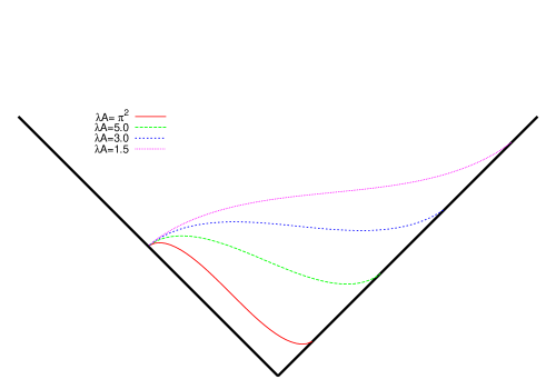
Figure 3: The profile functions corresponding to the density satisfying Wigner’s semi-circle law. As $\lambda A$ approaches to the critical area, $\lambda A_{c}=\pi^{2}$, the shape of the profile function becomes a rectangle. When the area becomes larger than the critical area, a line region would appear in the profile function. Note that the critical area dose not depend on the value of $m$.

To see the shape of the Young diagram which is dominated in the double scale limit, it is convenient to determine the profile function corresponding to it. By integrating the density (4.12) for $x$, we obtain

$$h^{-1}(x)=\begin{cases}0&\qquad(x<-R)\\ \displaystyle\frac{m}{\pi}\left[\arcsin\left(\frac{x}{R}\right)+\frac{x}{R}\sqrt{1-\left(\frac{x}{R}\right)^{2}}+\frac{\pi}{2}\right]&\qquad(-R\leq x\leq R)\\ m&\qquad(x>R)\end{cases}.$$ (4.15)

Substituting this into the continuous profile function (4.5), we can easily exhibit the shape of Young diagrams dominating in the double scaling limit. In Fig.3, we draw the shape of the profile function corresponding to the expression $\widetilde{h}(x)$ above. Here profiles are obtained with choosing appropriate $U(1)$ charge or the center $a$ to slide the profile function towards the oblique direction in order that the profiles fall into place.

In the figure, we see that a region where the derivative of the profile function is less than $-1$ appears when the area exceeds the critical area $\lambda A_{c}=\pi^{2}$. If we assume that this region is replaced by a line, $-x+const.$, we can understand this phase transition as a transition from the one-cut solution to a two-cut solution in the language of the density $\rho(x)$ [20].

5 Aspects from string theory

We have seen in the previous sections that a connection between 2D Yang-Mills theory on a sphere and the partition function of the 4D instanton counting. This connection is so mysterious only from the field theoretical point of view. However if we realize the 4D gauge theory in string theory using branes, the connection becomes to be clear.

Let us now consider $N$ D5-branes wrapping on a 2-cycle ($\mathbb{C}{\rm P}^{1}$) in an ALE space with resolved $A_{1}$ singularity in Type IIB superstring theory. This configuration preserves 8 supercharges on $\mathbb{R}^{1,3}$ worldvolume direction of D5-branes except for the 2-cycle and ${\cal N}{=}2$ $U(N)$ 4D gauge theory appears. And also, the internal theory on $\mathbb{C}{\rm P}^{1}$ must be topologically twisted and we expect that it is equivalent to a bosonic topological 2D Yang-Mills theory of the BF type as discussed in [31]

$$S=\int_{\mathbb{C}{\rm P}^{1}}\Phi F.$$ (5.1)

However, from the analysis of the double scaling limit in the section 4, the limit of 2D Yang-Mills has the quadratic potential as the $c=0$ matrix model below the Douglas-Kazakov phase transition point. This means that the action might be deformed to ${\cal N}{=}1$ by an induced quadratic potential

$$S=\int_{\mathbb{C}{\rm P}^{1}}\Phi F+\mu{\rm Tr}\,\Phi^{2}.$$ (5.2)

This theory reduces to an ordinary 2D Yang-Mills theory after integrating out $\Phi$. Geometrically, the 2-cycle $\mathbb{C}{\rm P}^{1}$ now turns into a 2-cycle in the resolved conifold.

The gauge coupling of the 4D theory is proportional to an area of the 2-cycle by a dimensional reduction, but the coupling could be complexified by adding the NS-NS B-field ($U(1)$ gauge field) through the 2-cycle which corresponds to the theta angle $\theta$. Namely, the gauge coupling of 4D theory and 2D objects are related each other by

$$2\pi i\tau=-\frac{\lambda A}{2}+i\theta.$$ (5.3)

In addition, the D5-branes have extra two dimensional transverse directions, which is identified with the vev of the adjoint scalar in the vector multiplet of ${\cal N}{=}2$ theory if we dropped the quadratic potential part in the large $N$ limit without fixing $\epsilon N$. The situation of the product group we have considered in section 3 corresponds to $N_{l}$ $(l=1,\ldots,r)$ D5-branes are localized at the same place of the transverse directions and the center of the D5-brane bunch is $a_{l}$. We need to take each large $N_{l}$ limit with fixing the center of positions and require that the near horizon radius does not overlap each other (each bunch should be sufficiently separated).

The instanton correction comes from the (euclidean) D-string wrapping around the blow-up 2-cycle. The $k$ instanton contribution corresponds to $k$ times wrapping D-string. Using the string like description of the 2D Yang-Mills partition function [16, 17, 18], wrapping maps from the world-volume of D-string to the target $\mathbb{C}{\rm P}^{1}$ are specified by the Young diagram (and related cycles). The Young diagram of each gauge factor is located at $a_{l}$ and it describes how to wrap D-strings on each localized $\mathbb{C}{\rm P}^{1}$ of the $N_{l}$ D5-branes. (See Fig.4.) The partition function (3.7) counts all possible configurations of the wrapping D-strings.

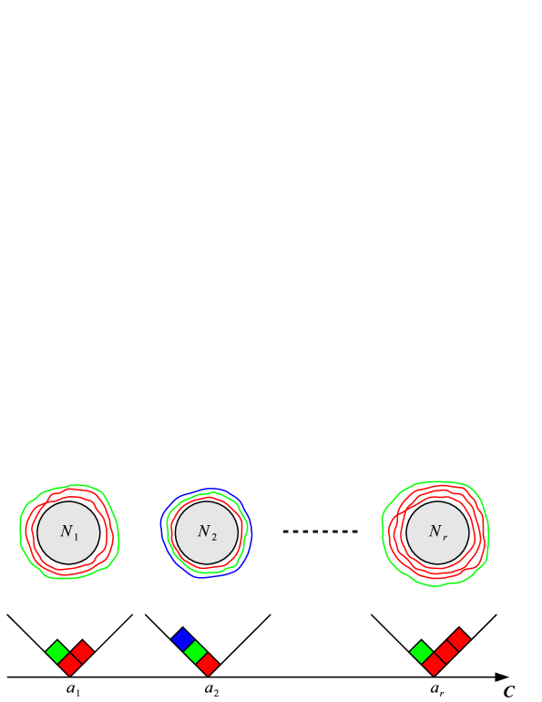
Figure 4: A configuration of instantons (wrapping D-strings). D-strings associated with the Young diagram are wrapping on $\mathbb{C}{\rm P}^{1}$ where D5-branes are wrapping on the same cycle.

According to the gauge/geometry (open/closed string) correspondence [2, 32, 33, 34, 35, 13], the large number limit of D-branes causes the geometry transition and D-brane charges turn to a non-trivial background flux. The flux carries all information of 4D ${\cal N}{=}2$ theory, that is, the information of the Seiberg-Witten geometry is encoded in the R-R and NS-NS B-filed flux configuration. This is regarded as a T-dual (along $x^{6}$) picture of the Hanany-Witten brane configuration [36, 37] in the large $N$ limit and also may relate to topological (closed) string theory on various geometry.

6 Conclusions and discussions

In this article, we discussed 2D Yang-Mills theory using the technique of the random partition. We found that the partition function of the 2D Yang-Mills theory can be written in terms of a “profile function” $f_{\bf k}(x|\epsilon)$ which expresses the Young diagram corresponding to the partition ${\bf k}$. We examined two kinds of limits of the theory; the large $N$ limit and the double scaling limit. We showed that the large $N$ limit of the partition function reproduces the partition function of the instanton counting of the 4D ${\cal N}=2$ supersymmetric gauge theory discovered by Nekrasov. On the other hand, we found that the double scaling limit of the partition function realizes naturally the discussion in Ref. [20] by Douglas and Kazakov. We also gave an interpretation of the instanton counting from the view point of brane configurations in the superstring theory.

We conclude this article by making some comments. In the section 3, we took the large $N$ limit of the 2D Yang-Mills theory on $S^{2}$ reproduces the instanton counting of a 4D ${\cal N}=2$ supersymmetric gauge theory. From this fact, it seems natural to expect that the double scaling limit of the 2D Yang-Mills theory discussed in the section 4 describes some non-perturbative aspects of a 4D theory. In fact, if the area is smaller than the critical area, the double scaling limit of the same theory is closely related to a $c=0$ matrix model. It suggests that the double scaling limit of 2D Yang-Mills theory might describe non-perturbative aspects of a 4D ${\cal N}=1$ supersymmetric gauge theory [13]. The deference between the partition function of the large $N$ limit and the double scaling limit is the cubic potential term $\int dxf_{{\bf k}}^{\prime\prime}(x|\epsilon)x^{3}$. If the cubic potential turns on, the ALE space where D5-branes live might be deformed to a Calabi-Yau manifold, which reduces the supersymmetry on the 4D space-time from ${\cal N}=2$ to ${\cal N}=1$. Moreover, if we admit this assumption, the phase transition discussed in Ref. [20] could be understood from the view point of the brane picture. In this picture, the area of $S^{2}$ where 2D Yang-Mills theory lives is that of a resolved 2-cycle in a CY manifold. When the area is small, the low energy theory on the D5-branes would be a 4D ${\cal N}=1$ supersymmetric gauge theory, which is consistent with the fact that the effective action of the 2D Yang-Mills theory is that of a $c=0$ matrix model in this parameter region. However, if the area becomes large enough, the effective theory on the D5-branes would not be a 4D theory but a 6D theory. The critical area might be identified with the area at which we cannot ignore the size of the $S^{2}$.

As for the phase transition, Gross and Witten have also discussed that a third order phase transition appears in the large $N$ limit of the one-plaquette model [38]. Recently, the authors in Ref. [26] have shown, among other things, that Willson’s one plaquette model can be formulated via the method of one-dimensional discrete random walk model which is also related to growing Young diagram, in which the authors argue that the Gross-Witten third order phase transition occurs when the growing Young diagram reaches its ceiling. It seems of quite interest to explore the relationship between the phase transition in the large $N$ limit of the one-plaquette model discussed by Gross and Witten [38] and the Douglas-Kazakov phase transition discussed in the section $4$.

References

- [1] G. ’t Hooft, A PLANAR DIAGRAM THEORY FOR STRONG INTERACTIONS, Nucl. Phys. B72 (1974) 461.
- [2] J. M. Maldacena, The large N limit of superconformal field theories and supergravity, Adv. Theor. Math. Phys. 2 (1998) 231–252 [hep-th/9711200].
- [3] E. Witten, Anti-de Sitter space and holography, Adv. Theor. Math. Phys. 2 (1998) 253–291 [hep-th/9802150].
- [4] S. S. Gubser, I. R. Klebanov and A. M. Polyakov, Gauge theory correlators from non-critical string theory, Phys. Lett. B428 (1998) 105–114 [hep-th/9802109].
- [5] O. Aharony, S. S. Gubser, J. M. Maldacena, H. Ooguri and Y. Oz, Large N field theories, string theory and gravity, Phys. Rept. 323 (2000) 183–386 [hep-th/9905111].
- [6] M. Fukuma, S. Matsuura and T. Sakai, Holographic renormalization group, Prog. Theor. Phys. 109 (2003) 489–562 [hep-th/0212314].
- [7] T. Eguchi and H. Kawai, Reduction of Dynamical Degrees of Freedom in the Large N Gauge Theory, Phys. Rev. Lett. 48 (1982) 1063.
- [8] D. J. Gross and Y. Kitazawa, A QUENCHED MOMENTUM PRESCRIPTION FOR LARGE N THEORIES, Nucl. Phys. B206 (1982) 440.
- [9] G. Bhanot, U. M. Heller and H. Neuberger, THE QUENCHED EGUCHI-KAWAI MODEL, Phys. Lett. B113 (1982) 47.
- [10] S. R. Das and S. R. Wadia, TRANSLATION INVARIANCE AND A REDUCED MODEL FOR SUMMING PLANAR DIAGRAMS IN QCD, Phys. Lett. B117 (1982) 228.
- [11] T. Banks, W. Fischler, S. H. Shenker and L. Susskind, M theory as a matrix model: A conjecture, Phys. Rev. D55 (1997) 5112–5128 [hep-th/9610043].
- [12] N. Ishibashi, H. Kawai, Y. Kitazawa and A. Tsuchiya, A large-N reduced model as superstring, Nucl. Phys. B498 (1997) 467–491 [hep-th/9612115].
- [13] R. Dijkgraaf and C. Vafa, A perturbative window into non-perturbative physics, hep-th/0208048.
- [14] A. A. Migdal, Recursion equations in gauge field theories, Sov. Phys. JETP 42 (1975) 413.
- [15] B. E. Rusakov, Loop averages and partition functions in U(N) gauge theory on two-dimensional manifolds, Mod. Phys. Lett. A5 (1990) 693–703.
- [16] D. J. Gross, Two-dimensional QCD as a string theory, Nucl. Phys. B400 (1993) 161–180 [hep-th/9212149].
- [17] D. J. Gross and I. Taylor, Washington, Two-dimensional QCD is a string theory, Nucl. Phys. B400 (1993) 181–210 [hep-th/9301068].
- [18] D. J. Gross and I. Taylor, Washington, Twists and Wilson loops in the string theory of two- dimensional QCD, Nucl. Phys. B403 (1993) 395–452 [hep-th/9303046].
- [19] S. Cordes, G. W. Moore and S. Ramgoolam, Lectures on 2-d Yang-Mills theory, equivariant cohomology and topological field theories, Nucl. Phys. Proc. Suppl. 41 (1995) 184–244 [hep-th/9411210].
- [20] M. R. Douglas and V. A. Kazakov, Large N phase transition in continuum QCD in two- dimensions, Phys. Lett. B319 (1993) 219–230 [hep-th/9305047].
- [21] J. A. Minahan and A. P. Polychronakos, Equivalence of two-dimensional QCD and the C = 1 matrix model, Phys. Lett. B312 (1993) 155–165 [hep-th/9303153].
- [22] S. Lelli, M. Maggiore and A. Rissone, Perturbative and non-perturbative aspects of the two- dimensional string / Yang-Mills correspondence, Nucl. Phys. B656 (2003) 37–62 [hep-th/0211054].
- [23] T. Matsuo and S. Matsuura, String theoretical interpretation for finite N Yang-Mills theory in two-dimensions, hep-th/0404204.
- [24] J. Baez and W. Taylor, Strings and two-dimensional QCD for finite N, Nucl. Phys. B426 (1994) 53–70 [hep-th/9401041].
- [25] C. Vafa, Two dimensional Yang-Mills, black holes and topological strings, hep-th/0406058.
- [26] S. de Haro and M. Tierz, Brownian motion, Chern-Simons theory, and 2d Yang-Mills, hep-th/0406093.
- [27] N. Nekrasov and A. Okounkov, Seiberg-Witten theory and random partitions, hep-th/0306238.
- [28] N. A. Nekrasov, Seiberg-Witten prepotential from instanton counting, hep-th/0306211.
- [29] N. A. Nekrasov, Seiberg-Witten prepotential from instanton counting, hep-th/0206161.
- [30] N. Seiberg and E. Witten, Monopoles, duality and chiral symmetry breaking in N=2 supersymmetric QCD, Nucl. Phys. B431 (1994) 484–550 [hep-th/9408099].
- [31] R. Dijkgraaf and C. Vafa, N = 1 supersymmetry, deconstruction, and bosonic gauge theories, hep-th/0302011.
- [32] R. Gopakumar and C. Vafa, Topological gravity as large N topological gauge theory, Adv. Theor. Math. Phys. 2 (1998) 413–442 [hep-th/9802016].
- [33] R. Gopakumar and C. Vafa, On the gauge theory/geometry correspondence, Adv. Theor. Math. Phys. 3 (1999) 1415–1443 [hep-th/9811131].
- [34] R. Dijkgraaf and C. Vafa, Matrix models, topological strings, and supersymmetric gauge theories, Nucl. Phys. B644 (2002) 3–20 [hep-th/0206255].
- [35] R. Dijkgraaf and C. Vafa, On geometry and matrix models, Nucl. Phys. B644 (2002) 21–39 [hep-th/0207106].
- [36] A. Hanany and E. Witten, Type IIB superstrings, BPS monopoles, and three-dimensional gauge dynamics, Nucl. Phys. B492 (1997) 152–190 [hep-th/9611230].
- [37] E. Witten, Solutions of four-dimensional field theories via M-theory, Nucl. Phys. B500 (1997) 3–42 [hep-th/9703166].
- [38] D. J. Gross and E. Witten, POSSIBLE THIRD ORDER PHASE TRANSITION IN THE LARGE N LATTICE GAUGE THEORY, Phys. Rev. D21 (1980) 446–453.