Quantum Oscillator on $\kern 2.0pt{\hbox{\sqi I}}\kern-4.2pt\rm CP^{n}$ in a constant magnetic field
Stefano Bellucci¹, Armen Nersessian^2,3 and Armen Yeranyan²

¹ INFN-Laboratori Nazionali di Frascati, P.O. Box 13, I-00044, Frascati, Italy
² Yerevan State University, Alex Manoogian St., 1, Yerevan, 375025, Armenia
³ Yerevan Physics Institute, Alikhanian Brothers St., 2, Yerevan, 375036, Armenia

Abstract

We construct the quantum oscillator interacting with a constant magnetic field on complex projective spaces $\kern 2.0pt{\hbox{\sqi I}}\kern-4.2pt\rm CP^{N}$, as well as on their non-compact counterparts, i. e. the $N-$dimensional Lobachewski spaces ${\cal L}_{N}$. We find the spectrum of this system and the complete basis of wavefunctions. Surprisingly, the inclusion of a magnetic field does not yield any qualitative change in the energy spectrum. For $N>1$ the magnetic field does not break the superintegrability of the system, whereas for $N=1$ it preserves the exact solvability of the system. We extend this results to the cones constructed over $\kern 2.0pt{\hbox{\sqi I}}\kern-4.2pt\rm CP^{N}$ and ${\cal L}_{N}$, and perform the (Kustaanheimo-Stiefel) transformation of these systems to the three-dimensional Coulomb-like systems.

Introduction

The harmonic oscillator plays a fundamental role in quantum mechanics. On the other hand, there are few articles related with the oscillator on curved spaces. The most known generalization of the Euclidian oscillator is the oscillator on curved spaces with constant curvature (sphere and hyperboloid) [1] given by the potential

$$V_{Higgs}=\frac{\omega^{2}r^{2}_{0}}{2}\frac{{\bf x}^{2}}{x^{2}_{0}},\qquad\epsilon{\bf x}^{2}+x^{2}_{0}=r^{2}_{0},\quad\epsilon=\pm 1.$$ (1)

This system received much attention since its introduction (see for a review [2] and refs. therein) and is presently known under the name of “Higgs oscillator”.

Recently the generalization of the oscillator to Kähler spaces has also been suggested, in terms of the potential [3]

$$V_{osc}=\omega^{2}g^{\bar{a}b}\partial_{\bar{a}}K\partial_{b}K.$$ (2)

Various properties of the systems with this potential were studied in Refs. [3, 4, 5, 6]. It was shown that on the complex projective spaces $\kern 2.0pt{\hbox{\sqi I}}\kern-4.2pt\rm CP^{N}$ such a system inherits the whole set of rotational symmetries and a part of the hidden symmetries of the $2N-$dimensional flat oscillator [3]. In Ref. [4], the classical solutions of the system on $\kern 2.0pt{\hbox{\sqi I}}\kern-4.2pt\rm CP^{2}$, ${\cal L}_{2}$ (the noncompact counterpart of $\kern 2.0pt{\hbox{\sqi I}}\kern-4.2pt\rm CP^{2}$) and the related cones were presented, and the reduction to three dimensions was studied. Particulary, it was found that the oscillator on some cone related with $\kern 2.0pt{\hbox{\sqi I}}\kern-4.2pt\rm CP^{2}$ (${\cal L}_{2}$) results, after Hamiltonian reduction, in the Higgs oscillator on the three-dimensional sphere (two-sheet hyperboloid) in the presence of a Dirac monopole field. In Ref. [5] we presented the exact quantum mechanical solutions for the oscillator on $\kern 2.0pt{\hbox{\sqi I}}\kern-4.2pt\rm CP^{2}$, ${\cal L}_{2}$ and related cones. We also reduced these quantum systems to three dimensions and performed their (Kustaanheimo-Stieffel) transformation to the three-dimensional Coulomb-like systems. The “Kähler oscillator” is a distinguished system with respect to supersymmetrisation as well. Its preliminary studies were presented in [6, 3].

In this paper we present the exact solution of the quantum oscillator on arbitrary-dimensional $\kern 2.0pt{\hbox{\sqi I}}\kern-4.2pt\rm CP^{N}$, ${\cal L}_{N}$ and related cones in the presence of a constant magnetic field. The study of such systems is not merely of academic interest. It is also relevant to the higher-dimensional quantum Hall effect. This theory has been formulated initially on the four-dimensional sphere [7] and further included, as a particular case, in the theory of the quantum Hall effect on complex projective spaces [8] (see, also [9]). The latter theory is based on the quantum mechanics on $\kern 2.0pt{\hbox{\sqi I}}\kern-4.2pt\rm CP^{N}$ in a constant magnetic field. Our basic observation is that the inclusion of the constant magnetic field does not break any existing hidden symmetries of the $\kern 2.0pt{\hbox{\sqi I}}\kern-4.2pt\rm CP^{N}$-oscillator and, consequently, its superintegrability and/or exact solvability are preserved.

To be more concrete, let us consider first the (classical) oscillator on $\rm I\kern-1.45pt\rm R^{2N}=\kern 2.0pt{\hbox{\sqi I}}\kern-4.2pt\rm C^{N}$. It is described by the symplectic structure

$$\Omega_{0}=d\pi_{a}\wedge dz^{a}+d{\bar{\pi}}_{a}\wedge d{\bar{z}}^{a}$$ (3)

and the Hamiltonian

$${\cal H}=\pi{\bar{\pi}}+\omega^{2}z\bar{z}.$$ (4)

It has a symmetry group $U(2n)$ given by the generators of $SO(2n)$ rotations

$$J^{+}_{ab}={\bar{z}}^{a}\pi_{b},\quad J^{-}_{\bar{a}\bar{b}}={z}^{a}\bar{\pi}_{b},\quad J_{a\bar{b}}=iz^{b}\pi_{a}-i\bar{\pi}_{b}\bar{z}^{a}$$ (5)

and the hidden symmetries

$$I^{+}_{ab}=\pi_{a}\pi_{b}+\omega^{2}\bar{z}^{a}\bar{z}^{b},\quad I^{-}=\bar{\pi}_{a}\bar{\pi}_{b}+\omega^{2}z^{a}z^{b},$$ (6)

$$I_{a\bar{b}}=\pi_{a}\bar{\pi}_{b}+\omega^{2}\bar{z}^{a}z^{b}.$$ (7)

The oscillator on the complex projective space $\kern 2.0pt{\hbox{\sqi I}}\kern-4.2pt\rm CP^{N}$ (for $N>1$) [3] and the one on Lobacewski space ${\cal L}_{N}$ are defined by the same symplectic structure as above, see eq. (3), with the Hamiltonian

$${\cal H}=g^{\bar{a}b}\bar{\pi}_{a}\pi_{b}+\frac{\omega^{2}{r^{2}_{0}}}{2}z\bar{z},\qquad g^{\bar{a}b}=\frac{2}{r^{2}_{0}}(1+\epsilon z\bar{z})(\delta^{ab}+\epsilon z^{a}{\bar{z}}^{b}),\qquad\epsilon=\pm 1.$$ (8)

The choice $\epsilon=1$ corresponds to $\kern 2.0pt{\hbox{\sqi I}}\kern-4.2pt\rm CP^{N}$, and $\epsilon=-1$ is associated to ${\cal L}_{N}$. This system inherits only part of the rotational and hidden symmetries of the $\kern 2.0pt{\hbox{\sqi I}}\kern-4.2pt\rm C^{N}$-oscillator given, respectively, by the following constants of motion:

$$J_{a\bar{b}}={i}(z^{b}\pi_{a}-\bar{\pi}_{b}\bar{z}^{a}),\quad I_{a\bar{b}}=2\frac{J^{+}_{a}J^{-}_{b}}{r^{2}_{0}}+\frac{\omega^{2}r^{2}_{0}}{2}{\bar{z}}^{a}z^{b}\;,$$ (9)

where $J^{+}_{a}={i}\pi_{a}+{i}\epsilon(\bar{z}\bar{\pi})\bar{z}^{a}$, $J_{a}^{-}=\bar{J}^{+}_{a}$ are the translation generators. It is clear that $J_{a\bar{b}}$ defines the $U(N)$ rotations, while $I_{a\bar{b}}$ is just a $\kern 2.0pt{\hbox{\sqi I}}\kern-4.2pt\rm CP^{N}$ counterpart of (7).
In order to include a constant magnetic field, we have to leave the initial Hamiltonian unchanged, and replace the initial symplectic structure (3) by the following one:

$$\Omega_{B}=\Omega+iBg_{a\bar{b}}dz^{a}\wedge d\bar{z}^{b},$$ (10)

where $g_{a\bar{b}}$ is a Kähler metric of the configuration space. It is easy to observe, that the inclusion of a constant magnetic field preserves only the symmetries of the $\kern 2.0pt{\hbox{\sqi I}}\kern-4.2pt\rm C^{N}$-oscillator generated by $J_{a\bar{b}}$ and $I_{a\bar{b}}$. On the other hand, the inclusion of the magnetic field preserves all the symmetries for the oscillator on $\kern 2.0pt{\hbox{\sqi I}}\kern-4.2pt\rm CP^{N}$. Hence, in the presence of a magnetic field the oscillators on $\kern 2.0pt{\hbox{\sqi I}}\kern-4.2pt\rm C^{N}$ and $\kern 2.0pt{\hbox{\sqi I}}\kern-4.2pt\rm CP^{N}$ look much more similar, than in its absence . Hence we could be sure that the $\kern 2.0pt{\hbox{\sqi I}}\kern-4.2pt\rm CP^{N}$- oscillator preserves its classical and quantum exact solvability in the presence of a constant magnetic field.

Below, we formulate the Hamiltonian and quantum-mechanical systems, describing the $\kern 2.0pt{\hbox{\sqi I}}\kern-4.2pt\rm CP^{N}$- and ${\cal L}_{N}$- oscillators in the constant magnetic field and present their wavefunctions and spectra. We also extend these results to the cones and discuss some related topics.

Oscillator in a constant magnetic field: $\kern 2.0pt{\hbox{\sqi I}}\kern-4.2pt\rm CP^{N}$ and ${\cal L}_{N}$

The classical Kähler oscillator in a constant magnetic field is defined by the Hamiltonian

$${{\cal H}}=g^{a\bar{b}}{\pi}_{a}{\bar{\pi}}_{b}+\omega^{2}g^{\bar{a}b}K_{\bar{a}}K_{b}\quad,$$ (11)

and the Poisson brackets corresponding to the symplectic structure (10)

$$\{\pi_{a},z^{b}\}=\delta^{b}_{a},\quad\{\bar{\pi}_{a},\bar{z}^{b}\}=\delta^{b}_{a},\quad\{\pi_{a},\bar{\pi}_{b}\}=iBg_{a\bar{b}}.$$ (12)

Its canonical quantization assumes the following choice of momenta operators:

$$\widehat{\pi}_{a}=-i\left(\hbar\partial_{a}+BK_{a}/2\right),\quad\widehat{\bar{\pi}}_{a}=-i\left(\hbar\partial_{\bar{a}}-BK_{\bar{a}}/2\right),$$ (13)

where $\partial_{a}=\partial/\partial z^{a}$, $\partial_{\bar{a}}=\partial/\partial{\bar{z}}^{a}$, $K_{a}=\partial K/\partial{z}^{a}$, $K_{\bar{a}}=\partial K/\partial{\bar{z}}^{a}$. The quantum Hamiltonian looks similar to the classical one

$$\widehat{{\cal H}}=\frac{1}{2}g^{a\bar{b}}(\widehat{\pi}_{a}\widehat{\bar{\pi}}_{b}+\widehat{\bar{\pi}}_{b}\widehat{\pi}_{a})+\omega^{2}g^{\bar{a}b}K_{\bar{a}}K_{b}.\quad$$ (14)

In the specific case of the complex projective space $\kern 2.0pt{\hbox{\sqi I}}\kern-4.2pt\rm CP^{N}$ and its noncompact version, i.e. the Lobacewski space ${\cal L}_{N}$, we have to choose

$$K=\frac{r^{2}_{0}}{2\epsilon}\log(1+\epsilon z\bar{z}),\qquad K_{a}=\frac{r^{2}_{0}}{2\epsilon}\frac{\bar{z}^{a}}{1+\epsilon z\bar{z}},\quad K_{\bar{a}}=\frac{r^{2}_{0}}{2\epsilon}\frac{z^{a}}{1+\epsilon z\bar{z}}.$$ (15)

The scalar curvature $R$ is related with the parameter $r^{2}_{0}$ as follows: $R=2\epsilon N(N+1)/r^{2}_{0}$. These systems possess the $u(N)$ rotational symmetry generators

$$\widehat{J}_{a\bar{b}}={i}\epsilon(z^{b}{\widehat{\pi}}_{a}-\bar{z}^{a}{\widehat{\bar{\pi}}}_{b})+{i}\epsilon(z^{c}\widehat{\pi}_{c}-\bar{z}^{c}\widehat{\bar{\pi}}_{c})\delta^{\bar{a}b}-\frac{Br^{2}_{0}}{2}\frac{\epsilon{\bar{z}}^{a}z^{b}-\delta^{\bar{a}b}}{1+\epsilon z\bar{z}},$$ (16)

and the hidden symmetry defined by the generators

$${\widehat{I}}_{a\bar{b}}=\frac{\widehat{{J}}^{+}_{a}\widehat{{J}}^{-}_{b}+\widehat{{J}}^{-}_{b}\widehat{{J}}^{+}_{a}}{r^{2}_{0}}+\frac{\omega^{2}r^{2}_{0}}{2}{\bar{z}}^{a}z^{b}\;,$$ (17)

where $\widehat{{J}}^{\pm}_{a}$ are the translations generators

$$\widehat{{J}}^{+}_{a}=i\widehat{\pi}_{a}+i\epsilon\bar{z}^{a}(\bar{z}\widehat{\bar{\pi}})-\frac{Br^{2}_{0}}{2}\frac{{\bar{z}}^{a}}{1+\epsilon z\bar{z}},\quad\widehat{{J}}^{-}_{a}=-i\widehat{\bar{\pi}}_{a}-i\epsilon z^{a}(z\widehat{\pi})-\frac{Br^{2}_{0}}{2}\frac{{z}^{a}}{1+\epsilon z\bar{z}}.$$ (18)

The Hamiltonian (14) could be rewritten as follows:

$${\cal H}=\frac{\hbar^{2}}{2r^{2}_{0}}\left[-\frac{(1+\epsilon x^{2})^{N+1}}{x^{2N-1}}\frac{\partial}{\partial x}\left(\frac{x^{2N-1}}{(1+\epsilon x^{2})^{N-1}}\frac{\partial}{\partial x}\right)+\frac{4(1+\epsilon x^{2})}{\epsilon x^{2}}{\widehat{\bf J}}^{2}+{\epsilon}(1+\epsilon x^{2})({2\widehat{J}_{0}}+\frac{\mu_{B}}{\epsilon})^{2}\right]+$$

$$+\frac{\omega^{2}r^{2}_{0}x^{2}}{2}-\epsilon\frac{\hbar^{2}\mu_{B}^{2}}{2r^{2}_{0}},$$ (19)

where

$$x=|z|,\quad\mu_{B}=\frac{Br^{2}_{0}}{2\hbar},\quad 2\widehat{J}_{0}=z^{a}\partial_{a}-\bar{z}^{\bar{a}}\partial_{\bar{a}},$$ (20)

$\widehat{\textbf{J}}^{2}$ is the quadratic Casimir of the $SU(N)$ momentum operator for the $N>1$, and $\widehat{\textbf{J}}=\widehat{J}_{0}$ for $N=1$. In order to get the energy spectrum of the system, let us consider the spectral problem

$$\widehat{{\cal H}}\Psi=E\Psi,\qquad\widehat{J}_{0}\Psi=s\Psi,\qquad\widehat{\bf J}^{2}\Psi=j(j+N-1)\Psi.$$ (21)

It is convenient to pass to the $2N-$dimensional spherical coordinates $(x,\phi_{i})$, where $i=1,\ldots,2N-1$, $x$ is a dimensionless radial coordinate taking values in the interval $[0,\infty)$ for $\epsilon=+1$, and in $[0,1]$ for $\epsilon=-1$, and $\phi_{i}$ are appropriate angular coordinates. The convenient algorithm for the expansion of “Cartesian” coordinates to the spherical ones is described in Appendix. In the new coordinates the above system could be solved by the following choice of the wavefunction:

$$\Psi=\psi(x)D^{j}_{s}(\phi_{i}),$$ (22)

where $D^{j}_{s}(\phi_{i})$ is the eigenfunction of the operators $\widehat{\bf J}^{2}$, $\widehat{J}_{0}$. It could be explicitly expressed via $2N-$dimensional Wigner functions, $D^{j}_{s}(\phi_{i})=\sum_{m_{i}}c_{m_{i}}D^{j}_{\{m-i\},s}(\phi_{i})$, where $j$, $m_{i}$ denote total and azimuth angular momenta, respectively, while $s$ is the eigenvalue of the operator $\widehat{J}_{0}$

$$m_{i},s=-j,-j+1,\ldots,j-1,j\;\;j=0,1/2,1,\ldots$$ (23)

Now, we make the substitution

$$x=\frac{\tan[\sqrt{\epsilon}\theta]}{\sqrt{\epsilon}},\quad\psi=\frac{f[\theta]\epsilon^{N/2-1/4}}{(\sin[\sqrt{\epsilon}\theta])^{N-1/2}(\cos[\sqrt{\epsilon}\theta])^{1/2}}$$ (24)

which yields the the following equation:

$$f^{\prime\prime}+\epsilon\left(\tilde{E}-\frac{j^{2}_{1}-1/4}{\sin^{2}[\sqrt{\epsilon}\theta]}-\frac{\delta^{2}-1/4}{\cos^{2}[\sqrt{\epsilon}\theta]}\right)f=0,$$ (25)

where

$$\tilde{E}=\frac{2Er^{2}_{0}}{\epsilon\hbar^{2}}+\frac{\omega^{2}r_{0}^{4}}{\hbar^{2}}+N^{2}+{\mu_{B}}^{2},\qquad\delta^{2}=\frac{\omega^{2}r_{0}^{4}}{\hbar^{2}}+\left(2s+\frac{\mu_{B}}{\epsilon}\right)^{2},\qquad j_{1}=2j+N-1.$$ (26)

The regular wavefunctions, which form a complete orthonormal of the above Schroedinger equation, are of the form

$$\psi=\left\{\begin{array}[]{c}C\sin^{j_{1}-1}\theta\cos^{\delta}\theta\;_{2}F_{1}(-n,n+\delta+j_{1}+1;j_{1}+1;\sin^{2}\theta),\;{\rm for\;}\epsilon=1\\ C\sinh^{j_{1}-1}\theta\cosh^{-\delta+2n}\theta\;_{2}F_{1}(-n,-n+\delta,j_{1}+1,\tanh^{2}\theta),\;{\rm for\;}\epsilon=-1,\end{array}\right.$$ (27)

where $n$ is the radial quantum number with the following range of definition:

$$n=\left\{\begin{array}[]{cc}0,1,\dots,\infty&{\rm for}\;\epsilon=1\\ 0,1,\dots,n^{max}=[(\delta-j_{1}-1)/2]&{\rm for}\;\epsilon=-1.\end{array}\right.$$ (28)

The normalization constants are defined by the expression

$$\frac{r_{0}^{2N}n!\Gamma^{2}(j_{1}+1)}{\Gamma(n+j_{1}+1)}C^{2}=\left\{\begin{array}[]{cc}(2n+j_{1}+1+\delta)\Gamma(n+j_{1}+1+\delta)/\Gamma(n+1+\delta),&{\rm for}\;\epsilon=1,\\ (\delta-2n-j_{1}-1)\Gamma(\delta-n)/\Gamma(\delta-n-j_{1}),&{\rm for}\;\epsilon=-1\;\;.\end{array}\right.$$ (29)

The energy spectrum reads

$$\tilde{E}=\left(2n+2j+N+\epsilon\delta\right)^{2},$$ (30)

or, explicitly,

$$E_{{n+j},\,s}=\frac{\epsilon\hbar^{2}}{2r^{2}_{0}}\left[\left(2n+2j+N+\epsilon\delta\right)^{2}-\left(\frac{\omega^{2}r_{0}^{4}}{\hbar^{2}}+N^{2}+{\mu_{B}}^{2}\right)\right].$$ (31)

The magnetic flux $\mu_{B}$ is quantised for $\epsilon=1$ and nonquantized for $\epsilon=-1$. In the flat limit $r^{2}_{0}\rightarrow\infty$ we get the correct formula for the $2N$-dimensional oscillator energy spectrum

$$E_{\tilde{n},s}=\hbar\sqrt{\omega^{2}+\frac{B^{2}_{0}}{4}}(\tilde{n}+N)+\hbar B_{0}s,\quad\tilde{n}=0,1,2,\ldots,$$ (32)

i.e. ${\tilde{n}}=2n+2j$ becomes the “principal” quantum number.

Thus, we get the following wonderful result: the inclusion of a constant magnetic field does not change the degeneracy of the oscillator’s spectrum on $\kern 2.0pt{\hbox{\sqi I}}\kern-4.2pt\rm CP^{N}$ and ${\cal L}_{N}$. For $N=1$, i.e. on the complex projective plane and Lobacewski plane, $s=j$, hence the spectrum is nondegenerate. For $N>1$ the spectrum depends on $s$ and $\tilde{n}\equiv 2n+2j$, i.e. it is degenerate in the orbital quantum number $j$. This degeneracy is due to the existence of a hidden symmetry. On the other hand, for $N=1$ the complex projective plane/Lobacewski plane coincides with the sphere/two-sheeted hyperboloid, while on these spaces there exists an oscillator system (Higgs oscillator) which possesses a hidden symmetry [1]. However, the inclusion of the constant magnetic field not only breaks the hidden symmetry (and the degeneracy of the energy spectrum) of that system, but makes it impossible to get the exact solution of its Schroedinger equation. So, opposite to the Higgs oscillator case, the Kähler oscillator on the two-dimensional sphere/hyperboloid behaves, with respect to the magnetic field, similarly to the planar one.

In free particle limit, i.e. for $\omega=0$, the energy spectrum is described by the principal quantum number $J$, which plays the role of the weight of the $SU(N+1)$ group (when $\epsilon=1$), and the $SU(N.1)$ group ( when $\epsilon=-1$). For example, when $\epsilon=1$, the energy spectrum is of the form

$$E_{{n+j},\,s}=\frac{2}{r^{2}_{0}}J(J+N)-\frac{\hbar^{2}}{2r^{2}_{0}}\mu_{B}^{2},\qquad J=n+j+|s+\frac{\mu_{B}}{2}|,\quad j\geq|s|.$$ (33)

As it is seen, the ground state becomes degenerate: the lowest value of $J$ is equal to $|{\mu_{B}}|/2$ (see [8] for details). Just this degeneracy plays a key role in the use of quantum mechanics on $\kern 2.0pt{\hbox{\sqi I}}\kern-4.2pt\rm CP^{N}$ in the theory of higher dimensional quantum Hall effect. For the details we refer to [8, 9] and related papers.

Conic oscillator

Our results could be easily extended to the family of $\nu-$ parametric cones (over $\kern 2.0pt{\hbox{\sqi I}}\kern-4.2pt\rm CP^{N}$ and ${\cal L}_{N}$) defined by the Kähler potential

$$K=\frac{r^{2}_{0}}{2\epsilon}\log(1+\epsilon(z\bar{z})^{\nu}),\quad\nu>0;\quad\epsilon=\pm 1.$$ (34)

The corresponding metric and oscillator potential are given by the expressions

$$g_{a\bar{b}}=\frac{\nu r^{2}_{0}(z\bar{z})^{\nu-1}}{2(1+\epsilon(z\bar{z})^{\nu})}\left(\delta_{a\bar{b}}-\frac{1-\nu+\epsilon(z\bar{z})^{\nu}}{z\bar{z}\;(1+\epsilon(z\bar{z})^{\nu})}\bar{z}^{a}z^{b}\right),\qquad V_{osc}=\frac{\omega^{2}r^{2}_{0}}{2}(z\bar{z})^{\nu}.$$ (35)

Introducing

$$(z\bar{z})^{{\nu}/2}=\frac{\tan[\sqrt{\epsilon}\theta]}{\sqrt{\epsilon}},\quad\psi=\frac{f[\theta]\epsilon^{N/2-1/4}}{(\sin[\sqrt{\epsilon}\theta])^{N-1/2}(\cos[\sqrt{\epsilon}\theta])^{1/2}}$$ (36)

and proceeding in a way completely similar to the previous case, we arrive to the equation (25), where $\tilde{E}$ is defined as in (26), while the parameters $\delta$ and $j_{1}$ look as follows:

$$\delta^{2}=\frac{\omega^{2}r_{0}^{4}}{\epsilon^{2}\hbar^{2}}+\left(2\frac{s}{\nu}+\frac{B_{0}r^{2}_{0}}{2\epsilon\hbar}\right)^{2}\qquad j^{2}_{1}=\frac{(2j+N-1)^{2}}{\nu}+\frac{\nu-1}{\nu}\left((N-1)^{2}-\frac{4s^{2}}{\nu}\right).$$ (37)

Thus, the wavefunctions and energy spectrum of the conic oscillator are defined, respectively, by the expressions (27),(28) and (30). The normalization constants $C_{cone}$ are of the form $C_{cone}=C/\nu^{N/2}$, where $C$ are defined by the expressions (29).

Explicitly, the energy spectrum of the conic oscillator reads

$$E_{n,\,j,\,s}=\frac{\epsilon\hbar^{2}}{2r^{2}_{0}}\left[(2n+j_{1}+1)^{2}+\frac{4s^{2}}{\nu^{2}}-N^{2}\right]+\frac{|\epsilon|\hbar^{2}}{r^{2}_{0}}\delta(2n+j_{1}+1)+\hbar B_{0}\frac{s}{\nu}\,.$$ (38)

KS-transformation

There is a well-known Kustaanheimo-Stiefel (KS) transformation [10] relating the four-dimensional oscillator with the three-dimensional Coulomb (and MIC-Kepler [11]) system. It allows for a straightforward extension to the oscillator on four-dimensional sphere $S^{4}$ and two-sheet hyperboloids $\rm I\kern-1.45pt\rm H_{4}$ [12], as well as on the $\kern 2.0pt{\hbox{\sqi I}}\kern-4.2pt\rm CP^{2}$, ${\cal L}_{2}$ and related cones [5]. The KS-transformation of the oscillator on $S^{4}$, $\rm I\kern-1.45pt\rm H_{4}$, $\kern 2.0pt{\hbox{\sqi I}}\kern-4.2pt\rm CP^{2}$, ${\cal L}_{2}$ yields the MIC-Kepler system on the three-dimensional two-sheet hyperboloid. The KS transformation of the oscillator on the cones over $\kern 2.0pt{\hbox{\sqi I}}\kern-4.2pt\rm CP^{2}$ and ${\cal L}_{2}$ results in the MIC-Kepler system on the three-dimensional cones over $\rm I\kern-1.45pt\rm H_{3}$ equipped with the metric (see [5] for details)

$$ds^{2}_{\nu,R^{2}_{0}}=\frac{8\nu R^{2}_{0}y^{2\sqrt{\nu}-2}(d{\bf y})^{2}}{(1-y^{2\sqrt{\nu}})^{2}},\qquad R_{0}=r^{2}_{0}.$$ (39)

The Hamiltonian of the system is given by the expression

$$\widehat{\cal H}_{MIC}=\frac{1}{\sqrt{g}}\widehat{\pi}_{i}{\sqrt{g}}g^{ij}\widehat{\pi}_{j}+s^{2}\hbar^{2}\frac{(1-y^{2\sqrt{\nu}})^{2}}{8\nu^{2}R^{2}_{0}y^{2\sqrt{\nu}}}-\frac{\gamma}{2R_{0}}\frac{1+y^{2\sqrt{\nu}}}{y^{\sqrt{\nu}}},$$ (40)

where

$$\widehat{\mbox{\boldmath$\pi$}}=-\imath\hbar\frac{\partial}{\partial{\bf y}}-s{\bf A(y)},\quad[\widehat{\pi}_{i},\widehat{\pi}_{j}]=\hbar s\epsilon_{ijk}\frac{y^{k}}{y^{3}}.$$ (41)

The coordinates of the initial and final systems are related as follows:

$${\bf y}=\left({\sqrt{1+\epsilon(z\bar{z})^{\nu}}-1}\right)^{2/\nu}\frac{z\mbox{\boldmath$\sigma$}\bar{z}}{(z\bar{z})^{2}}$$ (42)

The energy and coupling constant $\gamma$ of this system are defined by the energy and frequency of the respective four-dimensional oscillator. The quantum number $s=0,\pm 1/2,1,\ldots$ becomes a fixed parameter (the “monopole number”), and instead of (23) one has

$$j=|s|,|s|+1,\ldots;\qquad m=-j,-j+1,\ldots,j-1,j.$$ (43)

It appears, that applying the KS-transformation to the four-dimensional oscillator in a constant magnetic field, we have to get the modification of the MIC-Kepler system on the three-dimensional hyperboloid (and related cones), which nevertheless remains superintegrable (exactly solvable).

Surprisingly, repeating the whole procedure, one can find that the inclusion of the magnetic field in the initial system yields, in the resulting system, a redefinition of the coupling constant $\gamma$ and the energy ${\cal E}$ only

$$\gamma=\frac{E_{\rm osc}}{2}+\frac{\epsilon\hbar^{2}}{r^{2}_{0}}(1-\frac{s^{2}}{\nu^{2}})-\frac{B_{0}}{2\nu}\hbar s,\quad-2{\cal E}=\omega^{2}+\frac{\epsilon E_{osc}}{r^{2}_{0}}+\frac{\hbar^{2}}{r^{4}_{0}}(1+2\frac{s^{2}}{\nu^{2}})+\frac{\epsilon B_{0}}{r^{2}_{0}\nu}\hbar s.$$ (44)

Using the expressions (27), one can convert the energy spectrum of the oscillator in the energy spectrum of the MIC-Kepler system

$${\cal E}=-\frac{2\left(\gamma-\epsilon\hbar^{2}(2n+j_{1}+1)^{2}/(4R_{0})\right)^{2}}{\hbar^{2}(2n+j_{1}+1)^{2}}-\frac{\epsilon\gamma}{R_{0}}+\frac{\hbar^{2}}{2R^{2}_{0}},$$ (45)

where ${j}_{1}$ is defined by the expression (37).

Summary and Conclusion

Let us summarize our results. We have shown that the inclusion of a constant magnetic field preserves the hidden symmetries of the oscillator on the complex projective space $\kern 2.0pt{\hbox{\sqi I}}\kern-4.2pt\rm CP^{N}$, in its noncompact version, i. e. the Lobacewski space ${\cal L}_{N}$. We constructed the complete basis of the wavefunction of these systems and their spectra and found that the inclusion of a constant magnetic field does not change the qualitative quantum properties of those systems. Particulary, the inclusion of the magnetic field does not change the degeneracy of the energy spectra. These results are extended to the oscillators on cones related with $\kern 2.0pt{\hbox{\sqi I}}\kern-4.2pt\rm CP^{N}$ and ${\cal L}_{N}$. In some sense, we have shown that the oscillators on $\kern 2.0pt{\hbox{\sqi I}}\kern-4.2pt\rm CP^{N}$ and ${\cal L}_{N}$ (with and without constant magnetic field) are more similar to the oscillator on $\kern 2.0pt{\hbox{\sqi I}}\kern-4.2pt\rm C^{N}$ in presence of the constant magnetic field, than to the one in its absence. Another observation concerns the reduction of the four-dimensional oscillator and the three-dimensional Coulomb-like system (KS transformation): we found, to our surprise, that the oscillators with and without (constant) magnetic fields result in the equivalent Coulomb-like systems. Notice, that for the $N=1$ our system remains exactly solvable in the presence of magnetic field, though it has no hidden symmetries. In opposite to our model, the well-known Higgs oscillator on $\kern 2.0pt{\hbox{\sqi I}}\kern-4.2pt\rm CP^{N}$ and ${\cal L}_{N}$, looses its exact solvability property in the presence of constant magnetic field, while in it absence it has a hidden symmetries. So, one can suppose, that considered system would preserve the exact solvability also in noncommutative case. Such a modification seems to be interesting due to the interesting rotational properties of noncommutative quantum mechanics in the constant magnetic field, observed at first for the planar case [13] and later on extended to the two-dimensional sphere and hyperboloid [14]. While the noncommutative planar oscillator with constant magnetic field remains superintegrable [15], on the noncommutative spheres and hyperboloids only the particle systems without potential terms [15, 16].

Appendix: The choice of the angular coordinates

It is convenient to pass to spherical coordinates by the use of the so-called “Smorodinsky’s trees method”. Let us illustrate this method on the simplest cases of $N=2$ and $N=3$. Its extension to higher dimensions is straightforward. For choosing the appropriate angular coordinates we build Smorodinsky trees (fig.1).

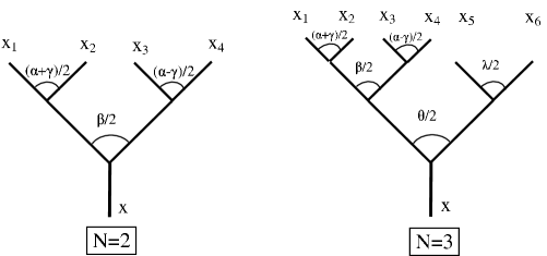
Figure 1: Smorodinsky trees for the cases N=2 and N=3.

By means of these trees we express the Cartesian coordinates $x_{1},\ldots,x_{2N}$, via spherical ones, $x,\phi_{i}$ by the following rules. The ends of the top of the branches mark Cartesian coordinates. The stock corresponds to the radial coordinate $x$. Each node marks some angle $\phi_{i}$. The angles marked by the top nodes have the range of definition $[0,2\pi)$, the remaining angles have the range of definition $[0,\pi/2)$. For the expansion of Cartesian coordinates in spherical ones we have to go to each top starting from the stock. When we are passing through a node (denoting the $\phi$ angle) to the left, we must write $\cos\phi$, whereas when passing through a node to the right, we must write $\sin\phi$.

Explicitly, one has
for $N=2$

$$z_{1} = x_{1}+{i}x_{2},\quad z_{2}=x_{3}+{i}x_{4};$$ (46)

$$x_{1} = x\cos[\beta/2]\cos[(\alpha+\gamma)/2],\quad x_{2}=x\cos[\beta/2]\sin[(\alpha+\gamma)/2],$$

$$x_{3} = x\sin[\beta/2]\cos[(\alpha-\gamma)/2],\quad x_{4}=x\sin[\beta/2]\sin[(\alpha-\gamma)/2].$$

$$\beta\in[0,\pi),\quad\alpha\in[0,4\pi),\quad\gamma\in[0,2\pi)$$

for $N=3$

$$z_{1} = x_{1}+{i}x_{2},\quad z_{2}=x_{3}+{i}x_{4},\quad z_{3}=x_{5}+{i}x_{6};$$ (47)

$$x_{1} = x\cos[\theta/2]\cos[\beta/2]\cos[(\alpha+\gamma)/2],\quad x_{2}=x\cos[\theta/2]\cos[\beta/2]\sin[(\alpha+\gamma)/2],$$

$$x_{3} = x\cos[\theta/2]\sin[\beta/2]\cos[(\alpha-\gamma)/2],\quad x_{4}=x\cos[\theta/2]\sin[\beta/2]\sin[(\alpha-\gamma)/2].$$

$$x_{5} = x\sin[\theta/2]\cos[\lambda/2],\quad x_{6}=x\sin[\theta/2]\sin[\lambda/2].$$

$$\beta,\theta\in[0,\pi),\quad\alpha,\lambda\in[0,4\pi),\quad\gamma\in[0,2\pi)$$

In these coordinates the operators $\bf{J}$ an $J_{0}$ look as follows:
for $N=2$

$$\bf{J}^{2} = -\frac{1}{\sin\beta}\frac{\partial}{\partial\beta}\left(\sin\beta\frac{\partial}{\partial\beta}\right)-\frac{1}{\sin^{2}\beta}\left[\frac{\partial^{2}}{\partial\alpha^{2}}+\frac{\partial^{2}}{\partial\gamma^{2}}-2\cos\beta\frac{\partial^{2}}{\partial\alpha\partial\gamma}\right],$$ (48)

$$J_{0} = -{i}\frac{\partial}{\partial\alpha},$$

for $N=3$

$$\bf{J}^{2} = -\frac{1}{\cos^{2}[\theta/2]}\left[\frac{1}{\sin\beta}\frac{\partial}{\partial\beta}\left(\sin\beta\frac{\partial}{\partial\beta}\right)+\frac{1}{\sin^{2}\beta}\left[\frac{\partial^{2}}{\partial\alpha^{2}}+\frac{\partial^{2}}{\partial\gamma^{2}}-2\cos\beta\frac{\partial^{2}}{\partial\alpha\partial\gamma}\right]\right]-$$

$$- \frac{1}{\sin^{2}[\theta/2]}\frac{\partial^{2}}{\partial\lambda^{2}}-\frac{1}{\cos^{3}[\theta/2]\sin[\theta/2]}\frac{\partial}{\partial\theta}\left(\cos^{3}[\theta/2]\sin[\theta/2]\frac{\partial}{\partial\theta}\right),$$

$$J_{0} = -{i}\left[\frac{\partial}{\partial\alpha}+\frac{\partial}{\partial\lambda}\right].$$

Without efforts this algorithm could be applied for any finite $N$.

References

• [1] P. W. Higgs, J. Phys. A12 (1979) 309; H. I. Leemon, J. Phys. A12 (1979) 489.
• [2] A. Barut, A. Inomata and G. Junker, J. Phys. A20 (1987) 6271; J. Phys. A23 (1990) 1179; D. Bonatos, C. Daskaloyanis and K. Kokkatos, Phys. Rev. A50 (1994) 3700; C. Grosche, G. S. Pogosyan and A. N. Sissakian, Fortschritte der Physik, 43 (6) (1995) 523; E. G. Kalnins, W. J. Miller and G. S. Pogosyan, Phys. Atom. Nucl.  65 (2002) 1086.
• [3] S. Bellucci and A. Nersessian, Phys. Rev. D67 (2003) 065013 .
• [4] A. Nersessian and A. Yeranyan, J. Phys.  A37 (2004) 2791.
• [5] S. Bellucci,A. Nersessian and A. Yeranyan, “Quantum Mechanics Model on Kaehler conifold” arXiv: hep-th/0312323 , to appear in Phys. Rev. D70 (15 July, 2004) issue 2.
• [6] S. Bellucci and A. Nersessian, “Supersymmetric Kaehler oscillator in a constant magnetic field,” arXiv:hep-th/0401232.
• [7] S. C. Zhang and J. P. Hu, Science 294 (2001) 823.
• [8] D. Karabali and V. P. Nair, Nucl. Phys. B641 (2002) 533.
• [9] B. A. Bernevig, J. P. Hu, N. Toumbas and S. C. Zhang, Phys. Rev. Lett.  91 (2003) 236803; M. Fabinger, JHEP 0205 (2002) 037; S. Bellucci, P. Y. Casteill and A. Nersessian, Phys. Lett.  B574 (2003) 121; D. Karabali and V. P. Nair, Nucl. Phys.  B679 (2004) 427; K. Hasebe and Y. Kimura, “Dimensional hierarchy in quantum Hall effects on fuzzy spheres”, arXiv:hep-th/0310274; D. Karabali and V. P. Nair, “Edge states for quantum Hall droplets in higher dimensions and a generalized arXiv:hep-th/0403111.
• [10] P. Kustaanheimo and E. Stiefel, J. Reine Angew Math. 218 (1965) 204; see, also the review V. Ter-Antonyan, Dyon-Oscillator Duality, arXiv:quant-ph 0003106.
• [11] D. Zwanziger, Phys. Rev. 176 (1968) 1480; H. V. McIntosh and A. Cisneros, J. Math. Phys. 11 (1970) 896.
• [12] A. Nersessian and G. Pogosyan, Phys. Rev. A63 (2001) 020103(R).
• [13] S. Bellucci, A. Nersessian and C. Sochichiu, Phys. Lett.  B522 (2001) 345.
• [14] S. Bellucci and A. Nersessian, Phys. Lett.  B542 (2002) 295.
• [15] V. P. Nair and A. P. Polychronakos, Phys. Lett.  B505 (2001) 267.
• [16] R. Iengo and R. Ramachandran, JHEP 0202 (2002) 017; D. Karabali, V. P. Nair and A. P. Polychronakos, Nucl. Phys. B627 (2002) 565.