hep-th/0406178

We present a noncommutative gauge theory that has the ordinary Standard Model as its low-energy limit. The model is based on the gauge group $U(4)\times U(3)\times U(2)$ and is constructed to satisfy the key requirements imposed by noncommutativity: the UV/IR mixing effects, restrictions on representations and charges of matter fields, and the cancellation of noncommutative gauge anomalies. At energies well below the noncommutative mass scale our model flows to the commutative Standard Model plus additional free $U(1)$ degrees of freedom which are decoupled due to the UV/IR mixing. Our model also predicts the values of the hypercharges of the Standard Model fields.

1 Introduction

One of the most novel and intriguing aspects of noncommutative gauge theories is the UV/IR mixing in which the physics of high-energy degrees of freedom affects the physics at low energies [4, 5]. Gauge theories on spaces with noncommuting coordinates,

$$[x^{\mu},x^{\nu}]=i\theta^{\mu\nu}\ ,$$ (1.1)

arise naturally as low-energy effective theories from string theory and D-branes, but they are also known to be extremely restrictive and difficult to use in particle physics model building due to a number of field-theoretical constraints imposed by noncommutativity:

1. the UV/IR mixing [4, 5] and decoupling of $U(1)$ degrees of freedom [6, 7];

2. the gauge groups are restricted to $U(N)$ groups [8, 9];

3. fields can transform only in (anti-)fundamental, bi-fundamental and adjoint representations of the gauge groups [10, 11, 12];

4. the charges of matter fields are restricted to $0$ and $\pm 1$, and this makes it difficult to give fractional electric charges to the quarks [13];

5. gauge anomalies cannot be cancelled in a chiral noncommutative theory, hence the anomaly-free theory must be vector-like [13, 10, 14].

The authors of Ref. [15] made an important step in noncommutative model building by proposing a noncommutative model which satisfies criteria 2, 3 and 4. Their model has the noncommutative gauge group $U(3)\times U(2)\times U(1)$ with matter fields transforming only in (bi-)fundamental representations, and remarkably, it predicts the hypercharges of the Standard Model. In many respects their model is similar to the bottom-up approach of [16] to the string embedding of the Standard Model in purely commutative settings. Unfortunately, the noncommutative $U(3)\times U(2)\times U(1)$ model of [15] is affected by the UV/IR mixing which causes the $U(1)$ hypercharge sector to decouple.

The motivation of this paper is to construct a noncommutative embedding of the Standard Model which satisfies all the requirements listed above. The model is based on the gauge group $U(4)\times U(3)\times U(2)$ with matter fields transforming in noncommutatively allowed representations. In the infrared the gauge group is spontaneously broken to the Standard Model group by a Higgs mechanism. We need a larger gauge group than the authors of [15] in order to incorporate the UV/IR mixing effects, yet remarkably we still find the correct values of the hypercharges for all the fields of the Standard Model.

Noncommutative field theories are defined by replacing the ordinary products of all fields in the Lagrangians of their commutative counterparts by the star-products

$$(\phi*\varphi)(x)\equiv\phi(x)\ e^{{i\over 2}\theta^{\mu\nu}\stackrel{{\scriptstyle\leftarrow}}{{\partial_{\mu}}}\stackrel{{\scriptstyle\rightarrow}}{{\partial_{\nu}}}}\ \varphi(x)\ .$$ (1.2)

In this way noncommutative theories can be viewed as field theories on ordinary commutative spacetime. For example, the noncommutative pure gauge theory action is

$$S_{\rm YM}[A]=-{1\over 2g^{2}}\int d^{4}x\ {\rm Tr}(F_{\mu\nu}*F_{\mu\nu})\ ,$$ (1.3)

where the commutator in the field strength also contains the star-product.

The UV/IR mixing in noncommutative theories arises from the fact that due to Eq. (1.2) certain Feynman diagrams acquire factors of the form $e^{ik_{\mu}\theta^{\mu\nu}p_{\nu}}$ (where k is an external momentum and p is a loop momentum) compared to their commutative counter-parts. At large values of the loop momentum $p$, the oscillations of $e^{ik_{\mu}\theta^{\mu\nu}p_{\nu}}$ improve the convergence of the loop integrals. However, as the external momentum vanishes, $k\to 0,$ the divergence reappears and what would have been a UV divergence is now reinterpreted as an IR divergence instead. This phenomenon of UV/IR mixing is specific to noncommutative theories and does not occur in the commutative settings where the physics of high energy degrees of freedom does not affect the physics at low energies.

Some of the earlier work on the phenomenology of noncommutative theories and on the noncommutative Standard Model (e.g. [17]) Taylor expands the exponential vertex factors which misses the physics of the UV/IR mixing. By Taylor-expanding the star-products in the Lagrangian, one obtains the action of the standard commutative theory plus an infinite number of $\theta$-dependent higher-derivative terms. At an energy-scale below the noncommutativity scale, $k^{2}\ll 1/\theta$, the higher-derivative terms correspond to irrelevant operators. One would naively expect that in the deep infrared one can simply drop all the effects due to irrelevant operators. This would imply that the noncommutative and the corresponding commutative theories belong to the same universality class, i.e. in the infrared their behaviour is identical. Classically the two theories are, in fact, identical in this regime. But at quantum level, this universality is broken due to the UV/IR mixing. The main point we are making, following [6, 4, 5] is that the effects of oscillating phases $e^{ik_{\mu}\theta^{\mu\nu}p_{\nu}}$ in Feynman diagrams can never be reproduced by the power-expansion in $\theta$.

Because of the breakdown of universality described above, one cannot apply the conventional picture and simply decouple completely the UV and IR sectors [4]. However, one can still calculate the Wilsonian effective action by integrating out the high-energy degrees of freedom and keeping track of the UV/IR mixing effects – following the approach initiated in [6].

The UV/IR mixing introduces new infrared divergencies into certain sectors of gauge theories on noncommutative spaces. In particular, this leads to quadratic and logarithmic IR divergencies in the polarisation tensor of $U(1)$ gauge fields, [5] which alter the dispersion relation of the photon. Fortunately, in a supersymmetric theory all quadratic divergences cancel and we are left only with logarithmic divergences [5, 6].

The remaining logarithmic divergencies were interpreted in [6, 7] as new contributions to the change of slope of the running coupling constant of the $U(1)$ sector of $U(N)$ gauge theories. In [7] the low-energy Wilsonian effective action for a large class of noncommutative supersymmetric theories was calculated and the results showed that the UV/IR mixing occurs only for the U(1) degrees of freedom which decouple (becoming unobservable) leaving a theory which at low energies looks like a safe commutative SU(N) theory. A similar decoupling between $U(1)$ and $SU(N)$ components of $U(N)$ was also observed in [9] for the one-loop gluon propagator in noncommutative QCD.

The conclusion one can draw from this is that it is conceivable to embed a commutative $SU(N)$ theory, such as e.g. QCD or the weak sector of the Standard Model into a supersymmetric noncommutative theory in the UV, but some extra care should be taken with the QED $U(1)$ sector. It is, in fact, pretty clear that the UV/IR mixing makes it impossible to interpret a noncommutative $U(1)$ theory as an ultraviolet embedding of ordinary QED. The low-energy theory emerging from the noncommutative $U(1)$ theory will become free in the extreme IR $k^{2}\to 0$ (rather than just weakly coupled) and in addition will have other pathologies. When supersymmetric theories are softly-broken down to ${\cal N}=0$ non-logarithmic IR divergences can re-appear. Models with the U(1) gauge group have been analysed [18, 19, 20] and tachyons can only be avoided if the model has ${\cal N}=4$ supersymmetry; even in this case the tachyons are avoided at the expense of giving a mass to the photon and fine tuning is required to keep this below experimental limits. The prospects for phenomenologically acceptable versions of such models looks bleak.

It is becoming pretty clear that the only realistic way to embed QED into noncommutative settings is to recover the electromagnetic $U(1)$ from a traceless diagonal generator of some higher $U(N)$ gauge theory. The trace-$U(1)$ part of this theory will decouple in the IR due to IR/UV mixing effects, and a traceless diagonal generator can give $U(1)$ as well as some non-Abelian $U(n)$ factors in favourable settings. So it seems that in order to embed QED into a noncommutative theory one should learn how to embed the whole Standard Model.

In the following section we will show how the UV/IR mixing leads to the decoupling of the overall $U(1)$ factors from the gauge groups in the infrared. (It should be noted however, that this decoupling is logarithmic and hence, slow.) In section 3 we will introduce the model, calculate the hypercharges, and discuss the gauge-, the fermion- and the Higgs-sectors. We will also outline how to cancel all the gauge anomalies by extending the model.

The model presented in this paper is one example of how the Standard Model can be embedded into a microscopic noncommutative gauge theory. One particularly interesting future direction would be to find a realistic supersymmetric version which would exhibit a dynamical supersymmetry breaking. This is motivated by the UV/IR-decoupled $U(1)$ degrees of freedom which provide a natural candidate for the hidden sector of dynamical supersymmetry breaking, as explained in [21].

2 UV/IR Mixing and the Decoupling of U(1)

In this section we will briefly recall how the UV/IR mixing effects in $U(N)$ noncommutative gauge theory lead to a decoupling of the overall $U(1)$ factor at energies below the noncommutative mass scale $M_{\scriptscriptstyle NC}\sim\theta^{-1/2}.$ Some more technical details related to our treatment of the UV/IR mixing are assembled in the Appendix which repeats the line of reasoning initiated in [6, 7].

We will first consider an unbroken $U(N)$ noncommutative theory with all matter fields transforming in the adjoint representation of the gauge group. The UV/IR mixing effects are present in the $U(1)$ sector, but do not affect the $SU(N)$ degrees of freedom, such that the leading order terms in the derivative expansion of the Wilsonian effective action read [7]:

$$L_{\rm eff}\ =\ -\frac{1}{2g^{2}_{\scriptscriptstyle U(1)}(k)}\ {\rm Tr}\,F^{\scriptscriptstyle U(1)}_{\mu\nu}F^{\scriptscriptstyle U(1)}_{\mu\nu}\ -\ \frac{1}{2g^{2}_{\scriptscriptstyle SU(N)}(k)}\ {\rm Tr}\,F^{\scriptscriptstyle SU(N)}_{\mu\nu}F^{\scriptscriptstyle SU(N)}_{\mu\nu}\ +\ \cdots\ ,$$ (2.1)

and the dots stand for terms involving matter fields and higher-derivative corrections. The multiplicative coefficients in front of the gauge kinetic terms in (2.1) define effective coupling constants of the corresponding gauge factors at momentum scale $k$. In the infrared we have effectively a matrix of $U(N)$ coupling constants:

$$\frac{1}{g_{\scriptscriptstyle U(N)}^{2}(k)}_{\scriptscriptstyle[N^{2}]\times[N^{2}]}\ =\ \frac{1}{g^{2}_{\scriptscriptstyle U(1)}(k)}\ \oplus\ \frac{1}{g_{\scriptscriptstyle SU(N)}^{2}(k)}\,\mbox{1 \kern-5.89996pt{\rm l}}_{\scriptscriptstyle[N^{2}-1]\times[N^{2}-1]}\$$ (2.2)

The running of the $SU(N)$ gauge coupling at 1-loop level is given by the same standard expression as in the commutative case,

$$\frac{(4\pi)^{2}}{g^{2}_{\scriptscriptstyle SU(N)}(k)}\,=\,b_{0}\,\log k^{2}\ ,$$ (2.3)

where $b_{0}$ is the first coefficient of the beta-function of the $SU(N)$ gauge theory. At the same time, the running of the $U(1)$ gauge coupling has the asymptotic behaviour [6]:

$$\frac{(4\pi)^{2}}{g^{2}_{\scriptscriptstyle U(1)}(k)} \rightarrow b_{0}\,\log k^{2}\ ,\qquad{\rm as}\ k^{2}\to\infty\ ,$$ (2.4)

$$\frac{(4\pi)^{2}}{g^{2}_{\scriptscriptstyle U(1)}(k)} \rightarrow -b_{0}\,\log{k^{2}}\ ,\qquad{\rm as}\ k^{2}\to 0\ ,$$ (2.5)

with the same $b_{0}$ as in (2.3).

It follows from (2.3),(2.4),(2.5) that the two effective coupling constants are identical in the UV and run in opposite directions in the IR as a result of the UV/IR mixing affecting the $U(1)$ sector [6, 7]. This leads to a breakdown of noncommutative $U(N)$ gauge symmetry, $U(N)\rightarrow U(1)\times SU(N),$ at momentum scales $k\leq M_{\scriptscriptstyle NC}\sim\theta^{-1/2}.$ The $U(1)$ degrees of freedom become weakly coupled and approach a free theory, $g_{\scriptscriptstyle U(1)}\rightarrow 0,$ as $k\rightarrow 0.$ The remaining $SU(N)$ degrees of freedom are described, at energies below $M_{\scriptscriptstyle NC},$ by the standard commutative gauge theory. At the same time, in the UV region, $k\gg M_{\scriptscriptstyle NC},$ the full noncommutative $U(N)$ gauge invariance is restored.

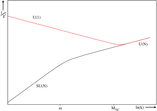
Figure 1: The running of the couplings in a softly-broken N=1 theory with one chiral multiplet in the adjoint representation.

To illustrate these results, Figure (1) shows how the coupling varies in a softly-broken ${\cal N}=1$ supersymmetric gauge theory with one chiral multiplet of mass $m$ transforming in the adjoint representation of $U(N)$. As can be seen from the graph, in the infrared regime of the theory, the gauge boson associated with the U(1) have decoupled [7].

It is worthwhile to note that what we have described here is a dynamical breakdown of noncommutative $U(N)$ at low energies, which is induced by different slopes of the running coupling constants. It is expected that when the higher derivative interactions are included in (2.1), the full noncommutative $U(N)$ gauge invariance will be recovered at the level of the effective action. More precisely, effective actions involving Wilson lines [22, 23, 24] can be written down which are explicitly gauge invariant [25, 26, 27] and which reduce to (2.1) when higher-derivative terms are dropped.

We will now summarise the consequences of the UV/IR mixing for more general cases relevant to considerations in this paper. First, one can include $N_{f}$ flavours of matter fields transforming in the fundamental representation of the gauge group, and, second, the gauge group $U(N)$ can be spontaneously broken to $U(n)$ at a scale $m$, so that some of the gauge bosons and matter fields become massive.

In the UV region, the theory is a noncommutative $U(N)$ and there is a single coupling constant,

$$\frac{(4\pi)^{2}}{g^{2}_{\scriptscriptstyle U(N)}(k)}\,\rightarrow\,b_{0}^{\scriptscriptstyle U(N)\,N_{f}}\,\log k^{2}\ ,\qquad{\rm as}\ k^{2}\to\infty\ .$$ (2.6)

Here $b_{0}^{\scriptscriptstyle U(N)\,N_{f}}$ is the 1-loop coefficient of the beta function of the microscopic $U(N)$ theory with $N_{f}$ fundamental flavours. In the IR region, two things happen: the trace $U(1)$ factor decouples below the noncommutative mass, and also, all the massive degrees of freedom freeze at momentum scales below their masses,

$$\frac{1}{g_{\scriptscriptstyle U(N)}^{2}(k)}\,\rightarrow\,\frac{1}{g^{2}_{\scriptscriptstyle U(1)}(k)}\ \oplus\ \frac{1}{g_{\scriptscriptstyle SU(n)}^{2}(k)}\,\mbox{1 \kern-5.89996pt{\rm l}}_{\scriptscriptstyle[n^{2}-1]\times[n^{2}-1]}\$$ (2.7)

where

$$\frac{(4\pi)^{2}}{g^{2}_{\scriptscriptstyle SU(n)}(k)} \rightarrow \,b_{0}^{\scriptscriptstyle SU(n)}\,\log k^{2}\ ,$$ (2.8)

$$\frac{(4\pi)^{2}}{g^{2}_{\scriptscriptstyle U(1)}(k)} \rightarrow \,-(2b_{0}^{\scriptscriptstyle U(N)\,N_{f}=0}-b_{0}^{\scriptscriptstyle U(N)\,N_{f}})\,\log{k^{2}}\ ,\qquad{\rm as}\ k^{2}\to 0\ .$$ (2.9)

The UV/IR mixing affects only the $U(1)$ coupling and, hence, the first equation (2.8) takes the standard commutative and recognizable form. However, the $U(1)$ coupling is affected by the UV/IR mixing and leads to the slope in the IR given by $-2b_{0}^{\scriptscriptstyle U(N)\,N_{f}=0}+b_{0}^{\scriptscriptstyle U(N)\,N_{f}}$ as follows from (2.9). This expression for the slope follows the fact that the $\theta$-dependent phase factors cancel in Feynman diagrams involving fundamental fields propagating in the loop [13] and do not cancel for adjoint fields in the loop.

Running couplings $\frac{1}{g^{2}(k)}$ of noncommutative $U(1)$ (supersymmetric) theories were first derived and plotted over the full range of the momentum scale $k$ in [6]. Our expressions in (2.6),(2.9) are in agreement with those results in the asymptotic regions $k^{2}\to\infty$ and $k^{2}\to 0$. It should be noted that expressions such as (2.9) are valid in the extreme infrared, at finite values of $k^{2}$ comparable to various mass scales in the theory, the coupling changes slopes.

In a non-supersymmetric, or softly broken supersymmetric gauge theory there are additional non-logarithmic sources of the UV/IR mixing effects which modify the dispersion relation for (decoupled) the $U(1)$ gauge field. Following [19], it can be shown that these contributions can be rendered harmless as long as two conditions are met. Firstly, for each fermion in the adjoint representation, there is a gauge field or complex scalar that is also in the adjoint representation (and vice-versa). This condition removes quadratic IR divergencies from the $U(1)$ polarisation tensor. Secondly the sum of the mass squared for the adjoint fermions must be less or equal than the sum of the mass squared for the complex scalars and the gauge bosons. If this condition is satisfied, there are no tachyons in the decoupled $U(1)$ gauge sector.

In the model that we outline in the next section, we can satisfy both these conditions hence the only consequence of the UV/IR mixing is that the U(1) degrees of freedom decouple in the extreme infrared. Even though the decoupling is only logarithmic, in this paper we will always assume that these trace-$U(1)$ degrees of freedom are completely decoupled and are essentially unobservable at low-energies. In much of what will follow the overall $U(1)$ factors of all three $U(N)$ gauge groups considered below will be dropped at energies much below the noncommutative scale relevant to the commutative Standard Model. The effects of these overall trace $U(1)$ degrees of freedom will be discussed in future work [33].

3 The Noncommutative Standard Model

As was mentioned earlier, all fields in a Noncommutative Gauge Theory must transform in the adjoint, fundamental, anti-fundamental or bi-fundamental representations. We assign the fields to the representations shown in table (1) and note that, unlike in the Standard Model, no field is charged under more than two groups. All the matter fermion fields come in three generations (which is not indicated explicitly in the table), and furthermore, the table will be extended in section 3.3.

Field $U_{C}(4)$ $U_{B}(3)$ $U_{A}(2)$ Hypercharge $e_{R}$ $\square$ -2 $\nu_{R}$ 0 $l_{L}=\left(\begin{matrix}\nu_{L}&e_{L}\end{matrix}\right)$ $\stackrel{{\scriptstyle-}}{{\square}}$ $\square$ -1 $u_{R}$ $\square$ $\stackrel{{\scriptstyle-}}{{\square}}$ $+\frac{4}{3}$ $d_{R}$ $\square$ $-\frac{2}{3}$ $q_{L}=\left(\begin{matrix}u_{L}&d_{L}\end{matrix}\right)$ $\square$ $\stackrel{{\scriptstyle-}}{{\square}}$ $+\frac{1}{3}$ $C_{\mu}$ $\square$$\stackrel{{\scriptstyle-}}{{\square}}$ 0 $B_{\mu}$ $\square$$\stackrel{{\scriptstyle-}}{{\square}}$ 0 $A_{\mu}$ $\square$$\stackrel{{\scriptstyle-}}{{\square}}$ 0 $\phi_{B}$ $\square$ 1 $\phi_{C\bar{B}}$ $\square$ $\stackrel{{\scriptstyle-}}{{\square}}$ $+\frac{1}{3}$ $\phi_{B\bar{A}}$ $\square$ $\stackrel{{\scriptstyle-}}{{\square}}$ $1$ $\phi_{A\bar{C}}$ $\stackrel{{\scriptstyle-}}{{\square}}$ $\square$ $-\frac{4}{3}$

Table 1: Representations for various fields in the theory

As can been seen from the table, we have introduced three bi-fundamental Higgs fields, $\phi_{A\bar{C}}$, $\phi_{C\bar{B}}$, $\phi_{B\bar{A}}$ and a fundamental $\phi_{B}$ compared to the Standard Model’s single fundamental Higgs. We note that unlike in [15] the scalar Higgs fields in our model are proper fields defined on the noncommutative space. Just like all other fields in the model, Higgs fields appear in the Lagrangian with the star-products. This is different from ”Higgsac” fields used in [15]. The latter have been shown to violate unitary [28].

The scalar potential (discussed in section 3.5) will induce the following VEV structure:

$$\langle\phi_{C\bar{B}}\rangle=\left(\begin{matrix}0&0&0\\ 0&0&0\\ 0&0&0\\ 0&0&a\end{matrix}\right)\quad\langle\phi_{B\bar{A}}\rangle=\left(\begin{matrix}\tilde{v}&0\\ 0&0\\ 0&b\\ \end{matrix}\right)\quad\langle\phi_{A\bar{C}}\rangle=\left(\begin{matrix}0&0&0&0\\ 0&0&0&c\end{matrix}\right)\quad\langle\phi_{B}\rangle=\left(\begin{matrix}0\\ v\\ 0\\ \end{matrix}\right)$$ (3.1)

The scalar potential will mean that the VEVs $a$, $b$ $c$ are much larger that $v$ and $\tilde{v}$ which will turn out to be the electroweak breaking scale.

The gauge bosons for the groups $U_{C}(4)$, $U_{C}(3)$ and $U_{C}(2)$ are respectively: $C^{p}_{\mu}$ ($p=0..15$), $B^{q}_{\mu}$ ($q=0..8$) and $A^{r}_{\mu}$ ($r=0..3$). So, for example, $\phi_{B}$ which transforms as

$$\phi_{B}\to U*\phi_{B}\phantom{with}U\in U_{B}(3)$$ (3.2)

will have a covariant derivative:

$$D_{\mu}*\phi_{B}=\partial_{\mu}*\phi_{B}+ig_{B}B_{\mu}^{q}t^{q}*\phi_{B}$$ (3.3)

and its Hermitian conjugate which transforms in the anti-fundamental, i.e.

$$\phi_{B}^{\dagger}\to\phi_{B}^{\dagger}*U^{-1}\phantom{with}U\in U_{B}(3)$$ (3.4)

will have a covariant derivative:

$$D_{\mu}*\phi_{B}^{\dagger}=\partial_{\mu}*\phi_{B}^{\dagger}-ig_{B}\phi_{B}^{\dagger}*B_{\mu}^{q}t^{q}$$ (3.5)

In the following discussion we will neglect the generator of the trace $U(1)$ of each group ($C^{0}_{\mu}$, $B^{0}_{\mu}$ and $A^{0}_{\mu}$) for simplicity. These generators will decouple at low-energies from the effective commutative Standard Model due to UV/IR mixing.

It should be noted however that the decoupling of the trace $U(1)$ factors from the $SU(N)$ degrees of freedom in the IR is logarithmic $g^{2}_{\scriptscriptstyle U(1)}\propto 1/\log k^{2}\rightarrow 0,$ and hence the $U(1)$ fields are decoupling slowly. It may well happen that the effects of these extra $U(1)$ degrees of freedom are not negligible and even important [33] for the low-energy physics at small non-vanishing momenta. In the rest of this paper and in particular in Section 3.1, for simplicity of presentation, we will always assume that these $U(1)$ degrees of freedom have completely decoupled from the low-energy effective theory.

3.1 The Gauge Sector

We start with the product of the three gauge groups, $U_{A}(2)\times U_{B}(3)\times U_{C}(4).$ Their couplings are denoted as $g_{\scriptscriptstyle A},$ $g_{\scriptscriptstyle B},$ and $g_{\scriptscriptstyle C},$ and their generators are ${\textstyle\frac{1}{2}}\sigma^{A},$ ${\textstyle\frac{1}{2}}\lambda^{B},$ and ${\textstyle\frac{1}{2}}T^{C}$ respectively. The vacuum expectation value for $\phi_{C\bar{B}}$ will partially break the gauge group. The covariant derivative is

$$D_{\mu}\langle\phi_{C\bar{B}}\rangle=\partial_{\mu}\langle\phi_{C\bar{B}}\rangle+\frac{i}{2}g_{C}C_{\mu}^{p}T^{p}*\langle\phi_{C\bar{B}}\rangle-\frac{i}{2}g_{B}\langle\phi_{C\bar{B}}\rangle*B_{\mu}^{q}\lambda^{q}$$ (3.6)

where, as mentioned earlier we have neglected the trace-$U_{C}(1)$ and $U_{B}(1)$ fields $C_{\mu}^{0}$ and $B_{\mu}^{0}$ due to their decoupling at low energies caused by the UV/IR mixing. It is in principle straightforward to incorporate these trace-$U(1)$ fields in the analysis, but we will not pursue this in the present paper. The $SU(4)$ generators ${\textstyle\frac{1}{2}}T^{1\dots 15}$ are listed in Appendix B and the $SU(3)$ generators ${\textstyle\frac{1}{2}}\lambda^{1\ldots 8}$ are taken to be the ${\textstyle\frac{1}{2}}$ Gell-Mann matrices.

The $\left(D_{\mu}\langle\phi_{C\bar{B}}\rangle\right)^{\dagger}\left(D_{\mu}\langle\phi_{C\bar{B}}\rangle\right)$ term in the Lagrangian will contain diagonal mass-terms:

$$\frac{a^{2}}{4}\bigg{(}g_{\scriptscriptstyle C}^{2}\left((C_{\mu}^{9})^{2}+(C_{\mu}^{10})^{2}+(C_{\mu}^{11})^{2}+(C_{\mu}^{11})^{2}+(C_{\mu}^{13})^{2}+(C_{\mu}^{14})^{2}\right)$$ (3.7)

$$+g_{\scriptscriptstyle B}^{2}\left((B_{\mu}^{4})^{2}+(B_{\mu}^{5})^{2}+(B_{\mu}^{6})^{2}+(B_{\mu}^{7})^{2}\right)\bigg{)}$$

and non-diagonal mass-terms:

$$\frac{a^{2}}{4}\left(\frac{3}{2}g_{\scriptscriptstyle C}^{2}(C_{\mu}^{15})^{2}+\frac{4}{3}g_{\scriptscriptstyle B}^{2}(B_{\mu}^{8})^{2}-2\sqrt{(}2)g_{\scriptscriptstyle B}g_{\scriptscriptstyle C}B_{\mu}^{8}C_{\mu}^{15}\right)$$ (3.8)

If we rotate to a new basis:

$$\left(\begin{matrix}M_{\mu}^{1}\\ M_{\mu}^{2}\end{matrix}\right)=\left(\begin{matrix}\mbox{cos}\,\theta_{CB}&\mbox{sin}\,\theta_{CB}\\ -\mbox{sin}\,\theta_{CB}&\mbox{cos}\,\theta_{CB}\end{matrix}\right)\left(\begin{matrix}C_{\mu}^{15}\\ B_{\mu}^{8}\end{matrix}\right)$$ (3.9)

where

$$\mbox{cos}\,\theta_{CB}=\frac{\sqrt{2}g_{\scriptscriptstyle B}}{\sqrt{2g_{\scriptscriptstyle B}^{2}+\frac{9}{4}g_{\scriptscriptstyle C}^{2}}}\qquad\mbox{sin}\,\theta_{CB}=\frac{\frac{3}{2}g_{\scriptscriptstyle C}}{\sqrt{2g_{\scriptscriptstyle B}^{2}+\frac{9}{4}g_{\scriptscriptstyle C}^{2}}}$$ (3.10)

Then $M_{\mu}^{1}$ will be massless but $M_{\mu}^{2}$ will acquire a mass so, out of the $U(4)\times U(3)$ that we start with, the following gauge bosons are still massless: $C^{1..8}_{\mu}$ (which we will identify with the $SU(3)_{C}$ of the Standard Model, $B^{1..3}_{\mu}$ (which we will identify with $SU(2)_{L}$) and $M^{1}_{\mu}$.

The covariant derivative for $\phi_{B\bar{A}}$ will lead to a term involving its vacuum expectation value. Because $\tilde{v}<<b$ (in equation (3.1)) we will temporarily set $\tilde{v}\to 0$

$$D_{\mu}\langle\phi_{B\bar{A}}\rangle=\partial_{\mu}\langle\phi_{B\bar{A}}\rangle+\frac{i}{2}g_{B}B^{q}_{\mu}\lambda^{q}*\langle\phi_{B\bar{A}}\rangle-\frac{i}{2}g_{A}\langle\phi_{C\bar{B}}\rangle*A^{r}_{\mu}\sigma^{r}$$ (3.11)

where the $SU(2)$ generators ${\textstyle\frac{1}{2}}\sigma^{r}$ are the usual ${\textstyle\frac{1}{2}}$ Pauli matrices. However, $B^{8}_{\mu}=\mbox{sin}\,\theta_{CB}M_{\mu}^{1}+\mbox{cos}\,\theta_{CB}M_{\mu}^{2}$ so ignoring the massive gauge bosons we have:

$$D_{\mu}\langle\phi_{B\bar{A}}\rangle=\partial_{\mu}\langle\phi_{B\bar{A}}\rangle+\frac{i}{2}g_{B}B_{\mu}^{q}\lambda^{q}*\langle\phi_{B\bar{A}}\rangle+\frac{i}{2}g_{0}M_{\mu}^{1}\lambda^{8}*\langle\phi_{B\bar{A}}\rangle-\frac{i}{2}g_{A}\langle\phi_{C\bar{B}}\rangle*A_{\mu}^{r}\sigma^{r}$$ (3.12)

where $g_{0}=g_{B}\mbox{sin}\,\theta_{CB}$ and now $q,r=1..3$.

The resulting diagonal mass-terms will be:

$$\frac{b^{2}}{4}\left(g_{\scriptscriptstyle A}^{2}\left((A_{\mu}^{1})^{2}+(A_{\mu}^{2})^{2}\right)\right)$$ (3.13)

and the remaining mass-terms are:

$$\frac{b^{2}}{4}\left(g_{\scriptscriptstyle A}^{2}(A_{\mu}^{3})^{2}+\frac{4}{3}g_{0}^{2}(M_{\mu}^{1})^{2}-\frac{4}{\sqrt{3}}g_{0}g_{\scriptscriptstyle A}(A_{\mu}^{3})(M_{\mu}^{1})\right)$$ (3.14)

We can diagonalise these by writing:

$$\left(\begin{matrix}Y_{\mu}\\ M_{\mu}^{3}\end{matrix}\right)=\left(\begin{matrix}\mbox{cos}\,\theta_{BA}&\mbox{sin}\,\theta_{BA}\\ -\mbox{sin}\,\theta_{BA}&\mbox{cos}\,\theta_{BA}\end{matrix}\right)\left(\begin{matrix}A_{\mu}^{3}\\ M_{\mu}^{1}\end{matrix}\right)$$ (3.15)

where

$$\mbox{cos}\,\theta_{BA}=\frac{\sqrt{3}g_{\scriptscriptstyle A}}{\sqrt{3g_{\scriptscriptstyle A}^{2}+4g_{0}^{2}}}\qquad\mbox{sin}\,\theta_{BA}=\frac{\frac{3}{2}g_{\scriptscriptstyle C}}{\sqrt{3g_{\scriptscriptstyle A}^{2}+4g_{0}^{2}}}$$ (3.16)

The field labelled $Y_{\mu}$ is the gauge boson for a massless $U(1)$ and will be identified with the hypercharge whilst the $M_{\mu}^{3}$ field has acquired a mass.

If we now calculate which gauge degrees of freedom are given a mass by $\phi_{A\bar{C}}$ it will turn out that no massless degrees of freedom acquire a mass; the gauge group is broken no further. In particular the $Y_{\mu}$ field remains unchanged.

To summarise, after decoupling the trace-$U(1)$ factors the group $SU_{C}(4)$ has been broken to $SU(3)\times U(1)$, $SU_{B}(3)$ has been broken to $SU(2)_{L}\times U(1)$ and $U_{A}(2)$ has been broken to $U(1)$. All of these $U(1)$ factors arise from traceless generators of $SU$ groups. Furthermore, only one linear combination of these three traceless $U(1)$’s remains massless. This single $U(1)$ group will now be identified with the hypercharge of the Standard Model.

3.2 Hypercharges

The hypercharge for each particle is determined by the representation of the particle under the microscopic gauge groups. The ideas in this section follow [16, 15] but because of our unusual gauge-group ($U(4)\times U(3)\times U(2)$) the details differ.

The coupling of the right handed electron (c.f table 1) to the hypercharge is determined by:

$$\bar{e}_{R}\gamma^{\mu}D_{\mu}e_{R}= \bar{e}_{R}\gamma^{\mu}\partial_{\mu}e_{R}+\frac{i}{2}g_{\scriptscriptstyle A}\bar{e}_{R}\gamma^{\mu}e_{R}A^{3}_{\mu}\sigma^{3}+\frac{i}{2}g_{\scriptscriptstyle A}\bar{e}_{R}\gamma^{\mu}[e_{R},A^{3}_{\mu}]\sigma^{3}$$ (3.17)

$$\bar{e}_{R}\gamma^{\mu}\partial_{\mu}e_{R}+\frac{i}{2}g_{\scriptscriptstyle A}\bar{e}_{R}\gamma^{\mu}e_{R}\mbox{sin}\,\theta_{BA}Y_{\mu}\sigma^{3}$$ (3.18)

We have ignored the $[e_{R},A^{3}_{\mu}]$ term as we are considering scales well below the noncommutative scale. The coupling between $Y_{\mu}$ and the particle in the first row of the U(2) doublet is therefore $g_{\scriptscriptstyle A}\mbox{sin}\,\theta_{BA}$. This should be proportional to the hypercharge, $-2g^{\prime}$ where we define $g^{\prime}\equiv\frac{1}{2}g_{\scriptscriptstyle A}\mbox{sin}\,\theta_{BA}$ to be the coupling to the hypercharge. With this definition, the hypercharge of all the other particles in the model is now fixed.

The right-handed down quark transforms in the fundamental of $U_{C}(4)$:

$$\bar{d}_{R}\gamma_{\mu}D_{\mu}d_{R}=\bar{d}_{R}\gamma_{\mu}\partial_{\mu}d_{R}+\frac{i}{2}g_{\scriptscriptstyle C}\bar{d}_{R}\gamma_{\mu}d_{R}T_{15}C_{\mu}^{15}+...$$ (3.19)

Writing $C_{\mu}^{15}=\mbox{cos}\,\theta_{CB}M_{\mu}^{1}-\mbox{sin}\,\theta_{CB}M_{\mu}^{2}$ and then $M_{\mu}^{1}=\mbox{cos}\,\theta_{BA}Y_{\mu}-\mbox{sin}\,\theta_{BA}N_{\mu}^{3}$ then the term that will determine the coupling is:

$$\frac{i}{2}g_{\scriptscriptstyle C}\bar{d}_{R}\gamma^{\mu}d_{R}T_{15}\mbox{cos}\,\theta_{CB}\mbox{cos}\,\theta_{BA}Y_{\mu}$$ (3.20)

So the coupling for the right-handed down quark (for all except the fourth particle in the multiplet) is:

$$Y_{d_{R}}=\frac{g_{\scriptscriptstyle C}}{\sqrt{6}}\mbox{cos}\,\theta_{CB}\mbox{cos}\,\theta_{BA}$$ (3.21)

Using equations (3.10) and (3.16) we find $\frac{Y_{d_{R}}}{g^{\prime}}=\frac{-2}{3}$ i.e. the Standard Model value.

We can calculate the hypercharges of the other particles in an analogous fashion. For example the multiplet of left-handed leptons has a term which can be written (ignoring massive fields):

$$=\frac{i}{2}\bar{\psi}_{L}^{l}\gamma_{\mu}\psi_{L}^{l}(g_{\scriptscriptstyle A}\sigma^{3}A_{\mu}^{3}-g_{sstB}B_{\mu}^{8}\lambda^{8})$$ (3.22)

$$=\frac{i}{2}\bar{\psi}_{L}^{l}\gamma_{\mu}\psi_{L}^{l}(g_{\scriptscriptstyle A}\sigma^{3}\mbox{sin}\,\theta_{BA}Y_{\mu}-g_{sstB}\lambda^{8}\mbox{sin}\,\theta_{CB}M_{\mu}^{1})$$

$$=\frac{i}{2}\bar{\psi}_{L}^{l}\gamma_{\mu}\psi_{L}^{l}(g_{\scriptscriptstyle A}\sigma^{3}\mbox{tan}\,\theta_{BA}\mbox{cos}\,\theta_{BA}-g_{sstB}\lambda^{8}\mbox{sin}\,\theta_{CB}\mbox{cos}\,\theta_{BA})Y_{\mu}$$

So the hypercharge of the left-handed leptons will be:

$$\frac{Y_{\psi_{L}^{l}}}{g^{\prime}} =\frac{\left(g_{\scriptscriptstyle A}\mbox{tan}\,\theta_{BA}-\frac{g_{sstB}}{\sqrt{3}}\mbox{sin}\,\theta_{CB}\right)\mbox{cos}\,\theta_{BA}}{\frac{1}{2}g_{\scriptscriptstyle A}\mbox{cos}\,\theta_{BA}\mbox{tan}\,\theta_{BA}}$$ (3.23)

$$=-1$$

The hypercharges of the other fields is listed in table (1) and each agrees with its Standard Model value.

3.3 Anomalies and Extra Fields

Anomalies have been thoroughly studied in a noncommutative context [13, 10, 14, 30]. The generally accepted conclusion is that in order for a noncommutative theory to be free of chiral anomalies, the theory must be vector-like.

The matter content introduced so far is chiral, as it must be in order to match the Standard Model matter content at low energies; we have left-handed (but no right-handed) fermions under the $U_{B}(3)$ gauge group that will become the $SU(2)_{L}$ group in the low-energy limit of the theory. To fix the problem we introduce three extra heavy generations, one for each observed generation. Each particle in these heavy generations must have the opposite chirality to their Standard Model counterpart.

Although these extra generations circumvent the problems with anomalies, this might also be possible by adding fewer fields to the theory. However, in the next section we will see that these extra heavy generations are essential when writing down the necessary Yukawa terms for the theory.

We must also add three more fields to the model. As discussed earlier there are two conditions that need to prevent quadratic divergences arising in the polarisation tensor of the decoupled U(1) gauge bosons. The first condition is that for each fermion in the adjoint representation of a gauge group, there is a gauge field or complex scalar that is also in the adjoint representation (and vice-versa). We have adjoint gauge fields but no adjoint matter so we add massive adjoint fermion fields, one per microscopic gauge group; $\lambda^{A}$, $\lambda^{B}$ and $\lambda^{C}$. Table 2 summarises the extra matter we have needed to add to the theory.

Field $U_{C}(4)$ $U_{B}(3)$ $U_{A}(2)$ Hypercharge $E_{L}$ $\square$ -2 $N_{L}$ 0 $L_{R}=\left(\begin{matrix}N_{R}&E_{R}\end{matrix}\right)$ $\stackrel{{\scriptstyle-}}{{\square}}$ $\square$ -1 $U_{L}$ $\square$ $\stackrel{{\scriptstyle-}}{{\square}}$ $+\frac{4}{3}$ $D_{L}$ $\square$ $-\frac{2}{3}$ $Q_{R}=\left(\begin{matrix}U_{R}&D_{R}\end{matrix}\right)$ $\square$ $\stackrel{{\scriptstyle-}}{{\square}}$ $+\frac{1}{3}$ $\lambda^{C}$ $\square$$\stackrel{{\scriptstyle-}}{{\square}}$ 0 $\lambda^{B}$ $\square$$\stackrel{{\scriptstyle-}}{{\square}}$ 0 $\lambda^{A}$ $\square$$\stackrel{{\scriptstyle-}}{{\square}}$ 0

Table 2: Representations for the ”extra” fields added to the theory

3.4 Yukawa Couplings

Unlike the Standard Model, multiple Higgs fields are required in order give mass to all the particles. The Yukawa terms can be arranged into two categories. Firstly, there are terms that involve fields from the same generation. Secondly, because we have generations with opposite chirality, we have novel terms involving fields from different generations. Additionally, as in the Standard Model, there can be the usual mixing between the generations but we neglect these here for simplicity.

Yukawa terms of the first type are (for one light generation):

$$\nu_{R}^{\dagger}\phi_{B\bar{A}}l^{L}_{A\bar{B}}+e^{R}_{A}\phi^{\dagger}_{\bar{B}}{l_{L}^{\dagger}}_{B\bar{A}}+q^{L}_{C\bar{B}}\phi_{B\bar{A}}{u_{R}^{\dagger}}_{A\bar{C}}+d^{R}_{C}\phi^{\dagger}_{\bar{B}}{q_{L}^{\dagger}}_{B\bar{C}}+\mbox{h.c}$$ (3.24)

and for a heavy generation:

$$N_{L}^{\dagger}\phi_{B\bar{A}}L^{R}_{A\bar{B}}+E^{L}_{A}\phi^{\dagger}_{\bar{B}}{L_{R}^{\dagger}}_{B\bar{A}}+Q^{R}_{C\bar{B}}\phi_{B\bar{A}}{U_{L}^{\dagger}}_{A\bar{C}}+D^{L}_{C}\phi^{\dagger}_{\bar{B}}{Q_{R}^{\dagger}}_{B\bar{C}}+\mbox{h.c}$$ (3.25)

These terms on their own are not sufficient to give large masses to all those particles which are not observed at low energies, for example there is a fourth ”colour” of quark that would not interact with the strong force, as the gauge group has been broken from $SU(4)$ to $SU(3)$ but would still interact electromagnetically.

The extra three generations in which each particle has the opposite chirality to its Standard Model equivalent (as introduced in section 3.3 to cure the problems with anomalies) also cures the problem here. The possible terms that mix a light generation with a heavy generation are:

$${E_{L}^{\dagger}}_{\bar{A}}\phi_{A\bar{C}}d^{R}_{C}+{L_{R}^{\dagger}}_{B\bar{A}}\phi_{A\bar{C}}q^{L}_{C\bar{B}}+N_{L}^{\dagger}\phi_{A\bar{C}}u^{R}_{C\bar{A}}+l^{L}_{A\bar{B}}\phi^{\dagger}_{B\bar{C}}{U_{L}^{\dagger}}_{C\bar{A}}+q^{L}_{C\bar{B}}\phi^{\dagger}_{B\bar{C}}N^{L}+\mbox{h.c.}$$ (3.26)

Notice that in the above generation-mixing terms (which violate baryon and lepton number) neither of the Higgses with an electroweak scale vacuum expectation appear, so leptoquark would only occur at a high energy scale, characterised by the $a$, $b$ and $c$ vacuum expectation values.

When all possible such Yukawa terms are included, the particle content of the model at low energies agrees with the observed spectrum of particles. Moreover the form of the coupling gives a natural explanation for the extremely small mass of the left-handed neutrino in the three light generations, the see-saw effect will naturally suppress their masses to be of order $\tilde{v}^{2}/a$ although there are enough parameters to keep the neutrinos in the three extra generations above the experimental bounds.

3.5 The Higgs Potential

The pattern of symmetry breaking and mass splittings in the preceding sections was dependent on a particular pattern (3.1) of vacuum expectation values for the Higgs fields. We now will construct a simple example of the scalar potential which generates the vev structure in Eq. (3.1).

First, using gauge transformations $SU_{B}(3)$, we put $\phi_{B}$ in the canonical form:

$$\langle\phi_{B}\rangle=\left(\begin{matrix}0\\ v\\ 0\\ \end{matrix}\right)\ .$$ (3.27)

Next, we require that $\phi^{\dagger}_{\bar{B}}\phi_{B\bar{A}}=0$ and further use the $SU_{A}(2)$ and $SU_{B}(2)$ transformations to diagonalise $\phi_{B\bar{A}}$:

$$\langle\phi_{B\bar{A}}\rangle=\left(\begin{matrix}\tilde{v}&0\\ 0&0\\ 0&b\\ \end{matrix}\right)\ .$$ (3.28)

Next we turn to $\phi_{C\bar{B}}$ and require that $\phi_{C\bar{B}}\phi_{B}=0.$ We also use $SU_{C}(4)$ to simplify $\phi_{C\bar{B}}$ further, such that:

$$\langle\phi_{C\bar{B}}\rangle=\left(\begin{matrix}0&0&0\\ 0&0&0\\ 0&0&f\\ g&0&a\end{matrix}\right)\ .$$ (3.29)

At this stage to achieve relatively simple expressions in (3.27),(3.28),(3.29), we have used all the available gauge symmetry and the orthogonality conditions which follow from the potential:

$$\lambda_{1}|\phi^{\dagger}_{\bar{B}}\phi_{B\bar{A}}|^{2}+\lambda_{2}|\phi_{C\bar{B}}\phi_{B}|^{2}\ .$$ (3.30)

This essentially leaves the third bi-fundamental Higgs unrestricted at this stage,

$$\langle\phi_{A\bar{C}}\rangle=\left(\begin{matrix}z_{1}&z_{2}&z_{3}&z_{4}\\ z_{5}&z_{6}&z_{7}&c\end{matrix}\right)\ .$$ (3.31)

Before imposing restrictions on $\phi_{A\bar{C}}$, we would like to first further simplify the expressions (3.27),(3.28),(3.29).

We introduce another term in the scalar potential,

$$\lambda_{3}\left({\cal D}_{B\bar{B}}-\mu_{1}^{2}\mbox{1 \kern-5.89996pt{\rm l}}_{B\bar{B}}\right)^{2}\ ,$$ (3.32)

where ${\cal D}_{B\bar{B}}$ is a bilinear combination of Higgs fields:

$${\cal D}_{B\bar{B}}\equiv\phi_{B\bar{A}}\phi^{\dagger}_{A\bar{B}}-\phi^{\dagger}_{B\bar{C}}\phi_{C\bar{B}}+\phi_{B}\phi^{\dagger}_{\bar{B}}\ .$$ (3.33)

On the right hand side of (3.33) the indices $\bar{A},A$ and $\bar{C},C$ are summed over, but not the indices $\bar{B},B$ which are left free, so that ${\cal D}_{B\bar{B}}$ transforms in the adjoint of $SU_{B}(3)$. The scalar potential (3.32) contains a trace over gauge indices, hence $\bar{B},B$ are finally summed over, and the Higgs potential (3.32) is a gauge singlet.

At the minimum of the potential (3.32) we have,

$$\left(\begin{matrix}|\tilde{v}|^{2}-|g|^{2}&0&-g^{\dagger}a\\ 0&|v|^{2}&0\\ -ga^{\dagger}&0&|b|^{2}-|a|^{2}-|f|^{2}\end{matrix}\right)=\left(\begin{matrix}\mu_{1}^{2}&0&0\\ 0&\mu_{1}^{2}&0\\ 0&0&\mu_{1}^{2}\end{matrix}\right)\ ,$$ (3.34)

and the vacuum solution is:

$$g=0\ ,\quad|\tilde{v}|^{2}=\mu_{1}^{2}=|v|^{2}\ ,\quad|b|^{2}-|a|^{2}-|f|^{2}=\mu_{1}^{2}\ .$$ (3.35)

We continue reducing the number of free parameters in the vev structure in a similar way to the considerations above and introduce another term in the scalar potential:

$$\lambda_{4}\left({\cal E}_{C\bar{C}}-\mu_{2}^{2}\mbox{1 \kern-5.89996pt{\rm l}}_{C\bar{C}}\right)^{2}\ ,$$ (3.36)

where ${\cal E}_{C\bar{C}}$ is defined as

$${\cal E}_{C\bar{C}}\ \equiv\ \phi_{C\bar{B}}\phi^{\dagger}_{B\bar{C}}\ =\ \left(\begin{matrix}0&0&0&0\\ 0&0&0&0\\ 0&0&|f|^{2}&fa^{\dagger}\\ 0&0&f^{\dagger}a&|a|^{2}\end{matrix}\right)\ .$$ (3.37)

The potential (3.36) is minimal at

$$a=\mu_{2}\ ,\qquad f=0\ ,$$ (3.38)

which complements the configuration (3.35).

We now return to the so far unconstrained Higgs field (3.31) and write down new terms in the scalar potential

$$\lambda_{5}\left({\cal G}_{A\bar{A}}-\mu_{1}^{2}\mbox{1 \kern-5.89996pt{\rm l}}_{A\bar{A}}\right)^{2}\ +\ \lambda_{6}\left({\cal K}_{C\bar{C}}\right)^{2}\ ,$$ (3.39)

where

$${\cal G}_{A\bar{A}}\equiv-\phi_{A\bar{C}}\phi^{\dagger}_{C\bar{A}}+\phi^{\dagger}_{A\bar{B}}\phi_{B\bar{A}}\ ,\quad{\cal K}_{C\bar{C}}\equiv\phi_{C\bar{B}}\phi^{\dagger}_{B\bar{C}}-\phi^{\dagger}_{C\bar{A}}\phi_{A\bar{C}}\ .$$ (3.40)

The minimum of (3.39) is

$$z_{1}=z_{2}=z_{3}=z_{4}=z_{5}=z_{6}=z_{7}=0\ ,\quad|c|^{2}=|a|^{2}=\mu_{2}^{2}\ ,\quad f=0\ .$$ (3.41)

The combined vacuum configuration gives

$$\langle\phi_{C\bar{B}}\rangle=\left(\begin{matrix}0&0&0\\ 0&0&0\\ 0&0&0\\ 0&0&\mu_{2}\end{matrix}\right)\quad\langle\phi_{B\bar{A}}\rangle=\left(\begin{matrix}\mu_{1}&0\\ 0&0\\ 0&\sqrt{\mu_{2}^{2}+\mu_{1}^{2}}\\ \end{matrix}\right)\quad\langle\phi_{A\bar{C}}\rangle=\left(\begin{matrix}0&0&0&0\\ 0&0&0&\mu_{2}\end{matrix}\right)\quad\langle\phi_{B}\rangle=\left(\begin{matrix}0\\ \mu_{1}\\ 0\\ \end{matrix}\right)$$

which reproduces (3.1).

Acknowledgements

We are grateful to Steve Abel, Anthony Owen, Andreas Ringwald, and especially Gabriele Travaglini for useful discussions. JL was supported by a PPARC Studentship and VVK by a PPARC Senior Fellowship.

Appendix A: UV/IR and the Polarisation Tensor

Our discussion here follows closely the formalism introduced in [6, 7], to which we refer the reader for further details. To derive the matrix of effective coupling constants, Eq. (2.2), we use a background perturbation theory and decompose the gauge field $A_{\mu}$ into a background field $B_{\mu}$ and a fluctuating quantum field $N_{\mu}$,

$$A_{\mu}=B_{\mu}+N_{\mu}\ \ .$$ (A.1)

The effective action $S_{\rm eff}(B)$ is obtained by functionally integrating over the fluctuating fields. Gauge invariance constrains the interactions which can be generated in this procedure. Therefore, the effective action will always contain the kinetic term

$$S_{\rm eff}(B)\ni-\frac{1}{2g^{2}_{\rm eff}}\int d^{4}x\ {\rm Tr}\left(F_{\mu\nu}*F_{\mu\nu}\right)\ \ .$$ (A.2)

The factor $\frac{1}{2g^{2}_{\rm eff}}$ on the right hand side is identified with the effective coupling constant at the momentum scale $k$ of the background field $B_{\mu}$. In order to determine $g_{\rm eff}$ it is sufficient to consider the kinetic term $(\partial_{\mu}B_{\nu}-\partial_{\nu}B_{\mu})^{2}$. In the effective Lagrangian, this term becomes

$$2\int\frac{d^{4}k}{(2\pi)^{4}}B_{\mu}^{A}(k)B_{\nu}^{B}(-k)\ \Pi_{\mu\nu}^{AB}(k)\ \ .$$ (A.3)

Equation (A.3) defines the polarization tensor $\Pi_{\mu\nu}^{AB}(k)$, which in the effective theory replaces the tree level transverse tensor $k^{2}\delta_{\mu\nu}-k_{\mu}k_{\nu}$. On general grounds, $\Pi_{\mu\nu}^{AB}(k)$ has the structure

$$\Pi_{\mu\nu}^{AB}(k)=\Pi_{1}^{AB}(k^{2},\tilde{k}^{2})(k^{2}\delta_{\mu\nu}-k_{\mu}k_{\nu})+\Pi_{2}^{AB}(k^{2},\tilde{k}^{2})\frac{\tilde{k}_{\mu}\tilde{k}_{\nu}}{\tilde{k}^{4}}\ \ .$$ (A.4)

The matrix of the running coupling constants in (2.2) is determined entirely by $\Pi_{1}^{AB}(k^{2},\tilde{k}^{2})$ via

$$\left[\frac{1}{g_{\rm eff}^{2}(k)}\right]^{AB}\ =\ \frac{\delta^{AB}}{g_{\rm micro}^{2}}\ +\ 4\Pi_{1}^{AB}(k^{2},\tilde{k}^{2})\ .$$ (A.5)

The term in (A.4) proportional to $\tilde{k}_{\mu}\tilde{k}_{\nu}/\tilde{k}^{4}$ would not appear in ordinary commutative theories. It is transverse and has derivative dimension $-2$; therefore it is of leading order compared to the standard gauge-kinetic term (which has derivative dimension $+2$), and leads to a power-like infrared singular behaviour. It is known that $\Pi_{2}$ vanishes for supersymmetric noncommutative gauge theories, as was first discussed in [5]. For nonsupersymmetric theories, $\Pi_{2}$ can potentially present serious problems. For our purposes however, it will be sufficient to note that for noncommutative theories with a matching number of bosonic and fermionic degrees of freedom transforming in the adjoint representation of $U(N)$, the term $\Pi_{2}$ is rendered harmless if a certain mass inequality relation is satisfied, [19]. Hence, for the rest of this Appendix we will concentrate mostly on $\Pi_{1}$.

The action functional which describes the dynamics of a spin-$j$ noncommutative field in the representation r of the gauge group in the background of $B_{\mu}$ has the general form [6, 31]

$$S[\phi] = -\int d^{4}x\ \phi_{m,a}*\left(-D^{2}(B)\delta_{mn}\delta^{ab}+2i(F_{\mu\nu}^{B})^{ab}{\textstyle\frac{1}{2}}J^{\mu\nu}_{mn}\right)*\phi_{n,b}$$ (A.6)

$$\equiv -\int d^{4}x\ \phi_{m,a}*[\Delta_{j,{\bf r}}]_{mn}^{ab}*\phi_{n,b}\ \ .$$ (A.7)

Here $a,b$ are indices of the representation r of noncommutative $U(N)$, $F^{ab}\equiv\sum_{A=1}^{N^{2}}F^{A}t^{A}_{ab}$, and $m,n$ are spin indices and $J^{\mu\nu}_{mn}$ are the generators of the euclidean Lorentz group appropriate for the spin of $\phi$:

$$J = 0\qquad\qquad\qquad\qquad{\rm for\ spin\ 0\ fields},$$ (A.8)

$$J^{\mu\nu}_{\rho\sigma} = i(\delta^{\mu}_{\rho}\delta^{\nu}_{\sigma}-\delta^{\nu}_{\rho}\delta^{\mu}_{\sigma})\qquad{\rm for\ 4\hbox{-}vectors},$$

$$[J^{\mu\nu}]_{\alpha}^{\ \beta} = i{\textstyle\frac{1}{2}}[\sigma^{\mu\nu}]_{\alpha}^{\ \beta}\qquad\qquad{\rm for\ Weyl\ fermions}\ \ .$$

At the one-loop level, the effective action is given by

$$S_{\rm eff}[B]=-\frac{1}{2g^{2}}\int d^{4}x\ {\rm Tr}F_{\mu\nu}*F_{\mu\nu}-\sum_{j,{\bf r}}\alpha_{j}\log{\rm det}_{*}\Delta_{j,{\bf r}}\ \ ,$$ (A.9)

where the sum is extended to all fields in the theory, including ghosts and gauge fields.

ghost real scalar Weyl fermion gauge field $\alpha_{j}$ 1 $-\frac{1}{2}$ $\frac{1}{2}$ $-\frac{1}{2}$ $d(j)$ 1 1 2 4 $C(j)$ 0 0 $\frac{1}{2}$ 2

Table 3: Constants for the various fields in the theory

Functional star-determinants are computed by

$$\begin{split}\log{\rm det}_{*}\Delta_{j,{\bf r}}\equiv&\log{\rm det}_{*}(-\partial^{2}+{\cal K}(B)_{j,{\bf r}})\\ &=\log{\rm det}_{*}(-\partial^{2})+{\rm tr}_{*}\log(1+(-\partial^{2})^{-1}{\cal K}(B)_{j,{\bf r}})\ .\end{split}$$ (A.10)

The first term on the second line of (A.10) contributes only to the vacuum loops and will be dropped in the following. The second term on the last line of (A.10) has an expansion in terms of Feynman diagrams.

Using this method and Eq. (A.3), one can write down the 1-loop expression for the vacuum polarisation tensor for the gauge bosons in a $U(N)$ noncommutative gauge theory with massless fields, all in the adjoint representation, [7],

$$\Pi^{AB}_{\mu\nu}(k)=\,{\textstyle\frac{1}{2}}\sum_{j}\alpha_{j}\int\!\frac{d^{d}p}{(2\pi)^{d}}\, \left[d(j)M^{AB}(k,p)\left(\frac{1}{2}\frac{(2p+k)_{\mu}(2p+k)_{\nu}}{p^{2}(p+k)^{2}}-\frac{\delta^{\mu\nu}}{p^{2}}\right)\right.$$

$$\left.+2C(j)M^{AB}(k,p)\frac{\delta^{\mu\nu}-k_{\mu}k_{\nu}}{p^{2}(p+k)^{2}}\right]$$ (A.11)

where we have introduced the tensor

$$M^{AB}(k,p)=(-d^{ALM}\sin\frac{k\tilde{p}}{2}+f^{ALM}\cos\frac{k\tilde{p}}{2})(d^{BML}\sin\frac{k\tilde{p}}{2}+f^{BML}\cos\frac{k\tilde{p}}{2})\ \ .$$ (A.12)

To proceed further on, we rewrite (A.12) using the relations [32]

$$f^{ALM}f^{BML} = -Nc_{A}\delta_{AB}\ \ ,$$

$$d^{ALM}d^{BML} = Nd_{A}\delta_{AB}\ \ ,$$

$$f^{ALM}d^{BML} = 0\ \ ,$$ (A.13)

where $c_{A}=1-\delta_{0A}$ and $d_{A}=2-c_{A}$. This way (A.12) collapses to

$$M^{AB}(k,p)=-N\ \delta^{AB}(1-\delta_{0A}\cos\tilde{k}{p})\ \ .$$ (A.14)

$\tilde{k}$ is defined as $\tilde{k}^{\nu}=k_{\mu}\theta^{\mu\nu}$. Loop integrals involving the first term in equation (A.14) give rise to the planar contribution and are analogous to their commutative counterparts. Integrals involving the second term in equation (A.14) give the non-planar contribution and cause the UV/IR mixing. Equation (A.14) already shows that it is exclusively degrees of freedom associated with the generator $T^{0}\propto\mbox{1 \kern-5.89996pt{\rm l}}$ that will exhibit the UV/IR mixing.

The sum in (A.11) extends over all particles in the adjoint representation that appear in the loop (gauge fields, ghosts, fermions and scalars). The constants $\alpha_{j}$, $d(j)$, and $C(j)$ are as shown in Table (3). Only matter in the adjoint representation is considered here because matter in the fundamental representation does not contribute to nonplanar diagrams.

Planar loop integrals are done in the dimensional regularisation, while nonplanar ones are UV-finite and are calculated directly in 4 dimensions. Nonplanar integrals are performed using

$$\int\frac{d^{4}p}{(2\pi)^{4}}\frac{e^{ip\tilde{k}}}{p^{2}(p+k)^{2}} = \frac{2}{(4\pi)^{2}}\int_{0}^{1}dx\ K_{0}(\sqrt{k^{2}x(1-x)}|\tilde{k}|)\ \ ,$$ (A.15)

$$\int\frac{d^{4}p}{(2\pi)^{4}}\frac{e^{ip\tilde{k}}}{p^{2}} = \frac{1}{(4\pi)^{2}}\frac{4}{\tilde{k}^{2}}\ \ ,$$ (A.16)

where the Bessel function $K_{0}(z)$ has a small-$z$ expansion

$$K_{0}(z)=-\log\frac{z}{2}\left[1+\frac{z^{2}}{4}+O(z^{4})\right]-\gamma_{E}-(\gamma_{E}-1)\frac{z^{2}}{4}+O(z^{4})\ \ ,$$ (A.17)

while for large-$z$ it is exponentially suppressed. Using (A.4) and (A.11), planar contributions to $\Pi_{1}^{AB}$ are given by

$${\Pi_{1}^{AB}}_{\rm planar}=\,\frac{\delta^{AB}}{4(4\pi)^{2}}\int_{0}^{1}dx\,b_{0}\,\log(k^{2}x(1-x))\ ,$$ (A.18)

and nonplanar ones are

$${\Pi_{1}^{AB}}_{\rm nonplanar}=\,\frac{\delta^{A0}\delta^{B0}}{4(4\pi)^{2}}\int_{0}^{1}dx\,2b_{0}\,K_{0}\left(\sqrt{k^{2}x(1-x)}|\tilde{k}|\right)\ ,$$ (A.19)

Now, using the definition of the running couplings (A.5), and the expansion (A.17) we derive the asymptotic expressions (2.3),(2.4),(2.5).

In order to generalise to $N_{f}\neq 0$ of fundamental flavours of matter fields, we only need to recall that the fundamental fields in the loops do not contribute to $\theta$-dependent diagrams, i.e. they contribute only to planar diagrams. Hence,

$${\Pi_{1}^{AB}}_{\rm planar} = \frac{\delta^{AB}}{4(4\pi)^{2}}\int_{0}^{1}dx\,b_{0}^{N_{f}\neq 0}\,\log(k^{2}x(1-x))\ ,$$ (A.20)

$${\Pi_{1}^{AB}}_{\rm nonplanar} = \frac{\delta^{A0}\delta^{B0}}{4(4\pi)^{2}}\int_{0}^{1}dx\,2b_{0}^{N_{f}=0}\,K_{0}\left(\sqrt{k^{2}x(1-x)}|\tilde{k}|\right)\ .$$ (A.21)

In order to include spontaneously broken gauge groups we need to add masses to gauge bosons,

$$\Pi^{AB}_{\mu\nu}(k)=\,{\textstyle\frac{1}{2}}\sum_{j}\alpha_{j}\int\!\frac{d^{d}p}{(2\pi)^{d}}\, \left[d(j)M^{AB}(k,p)\left(\frac{1}{2}\frac{(2p+k)_{\mu}(2p+k)_{\nu}}{(p^{2}+m^{2})[(p+k)^{2}+m^{2}]}-\frac{\delta^{\mu\nu}}{p^{2}+m^{2}}\right)\right.$$

$$\left.+2C(j)M^{AB}(k,p)\frac{\delta^{\mu\nu}-k_{\mu}k_{\nu}}{(p^{2}+m^{2})[(p+k)^{2}+m^{2}]}\right]$$ (A.22)

but it is important to note that the gauge boson masses depend on $L$ and $M$ indices in (A.12), and one should use (A.12) rather than (A.14) for $M^{AB}$. In order to proceed, we represent the final answer for $\Pi^{AB}_{\mu\nu}(k)$ as the contribution of the unbroken (massless) $U(N)$, plus the correction, originating from

$$\begin{split}\int d^{4}p\left(\frac{1}{(p^{2}+m_{L}^{2})[(p+k)^{2}+m_{M}^{2}]}-\frac{1}{p^{2}(p+k)^{2}}\right)\\ \times\left(f^{ALM}f^{BML}\cos^{2}\frac{\tilde{k}p}{2}-d^{ALM}d^{BML}\sin^{2}\frac{\tilde{k}p}{2}\right)\ .\end{split}$$ (A.23)

The expression on the right hand side is UV-convergent in 4 dimensions, and one can set $\tilde{k}=0$, i.e. remove the nonplanar effective UV cut-off $\Lambda_{UV}=1/\tilde{k}$. This is equivalent to saying that for $\tilde{k}^{2}\to 0$, the $\log(\tilde{k})$ terms will cancel in the integral. What is left after that is the standard $\theta$-independent expression which corrects the planar $SU(N)$ running from a massless to a massive case. This has nothing to do with the $U(1)$ running coupling which is simply given by the massless contribution. From this reasoning, Eqs. (2.8),(2.9) follow.

Appendix B: Generators of SU(4)

Throughout this paper, the generators of SU(4) are $t^{a}=\frac{1}{2}T^{a}$ where $a=1..15$ and the $T^{a}$ are:

$$T_{1}= \left(\begin{matrix}0&1&0&0\\ 1&0&0&0\\ 0&0&0&0\\ 0&0&0&0\\ \end{matrix}\right) T_{2}= \left(\begin{matrix}0&-i&0&0\\ i&0&0&0\\ 0&0&0&0\\ 0&0&0&0\\ \end{matrix}\right) T_{3}= \left(\begin{matrix}1&0&0&0\\ 0&-1&0&0\\ 0&0&0&0\\ 0&0&0&0\\ \end{matrix}\right)$$

$$T_{4}= \left(\begin{matrix}0&0&1&0\\ 0&0&0&0\\ 1&0&0&0\\ 0&0&0&0\\ \end{matrix}\right) T_{5}= \left(\begin{matrix}0&0&-i&0\\ 0&0&0&0\\ i&0&0&0\\ 0&0&0&0\\ \end{matrix}\right) T_{6}= \left(\begin{matrix}0&0&0&0\\ 0&0&1&0\\ 0&1&0&0\\ 0&0&0&0\\ \end{matrix}\right)$$

$$T_{7}= \left(\begin{matrix}0&0&0&0\\ 0&0&-i&0\\ 0&i&0&0\\ 0&0&0&0\\ \end{matrix}\right) T_{8}=\frac{1}{\sqrt{3}} \left(\begin{matrix}1&0&0&0\\ 0&1&0&0\\ 0&0&-2&0\\ 0&0&0&0\\ \end{matrix}\right) T_{9}= \left(\begin{matrix}0&0&0&1\\ 0&0&0&0\\ 0&0&0&0\\ 1&0&0&0\\ \end{matrix}\right)$$

$$T_{10}= \left(\begin{matrix}0&0&0&i\\ 0&0&0&0\\ 0&0&0&0\\ -i&0&0&0\\ \end{matrix}\right) T_{11}= \left(\begin{matrix}0&0&0&0\\ 0&0&0&1\\ 0&0&0&0\\ 0&1&0&0\\ \end{matrix}\right) T_{12}= \left(\begin{matrix}0&0&0&0\\ 0&0&0&i\\ 0&0&0&0\\ 0&-i&0&0\\ \end{matrix}\right)$$

$$T_{13}= \left(\begin{matrix}0&0&0&0\\ 0&0&0&0\\ 0&0&0&1\\ 0&0&1&0\\ \end{matrix}\right) T_{14}= \left(\begin{matrix}0&0&0&0\\ 0&0&0&0\\ 0&0&0&i\\ 0&0&-i&0\\ \end{matrix}\right) T_{15}=\frac{1}{\sqrt{6}} \left(\begin{matrix}1&0&0&0\\ 0&1&0&0\\ 0&0&1&0\\ 0&0&0&-3\\ \end{matrix}\right)$$

References

• [1] N. Seiberg and E. Witten, “String theory and noncommutative geometry,” JHEP 9909 (1999) 032, hep-th/9908142.
• [2] M. R. Douglas and N. A. Nekrasov, “Noncommutative field theory,” Rev. Mod. Phys.  73 (2001) 977, hep-th/0106048.
• [3] R. J. Szabo, “Quantum field theory on noncommutative spaces,” Phys. Rept.  378 (2003) 207, hep-th/0109162.
• [4] S. Minwalla, M. Van Raamsdonk and N. Seiberg, “Noncommutative perturbative dynamics,” JHEP 0002 (2000) 020, hep-th/9912072.
• [5] A. Matusis, L. Susskind and N. Toumbas, “The IR/UV connection in the noncommutative gauge theories,” JHEP 0012 (2000) 002, hep-th/0002075.
• [6] V. V. Khoze and G. Travaglini, “Wilsonian effective actions and the IR/UV mixing in noncommutative gauge theories,” JHEP 0101 (2001) 026, hep-th/0011218.
• [7] T. J. Hollowood, V. V. Khoze and G. Travaglini, “Exact results in noncommutative N = 2 supersymmetric gauge theories,” JHEP 0105 (2001) 051, hep-th/0102045.
• [8] K. Matsubara, “Restrictions on gauge groups in noncommutative gauge theory,” Phys. Lett. B 482 (2000) 417, hep-th/0003294.
• [9] A. Armoni, “Comments on perturbative dynamics of non-commutative Yang-Mills theory,” Nucl. Phys. B593 (2001) 229, hep-th/0005208.
• [10] J. M. Gracia-Bondia and C. P. Martin, “Chiral gauge anomalies on noncommutative R**4,” Phys. Lett. B 479 (2000) 321 [arXiv:hep-th/0002171].
• [11] S. Terashima, “A note on superfields and noncommutative geometry,” Phys. Lett. B 482 (2000) 276 [arXiv:hep-th/0002119].
• [12] M. Chaichian, P. Presnajder, M. M. Sheikh-Jabbari and A. Tureanu, “Noncommutative gauge field theories: A no-go theorem,” Phys. Lett. B 526 (2002) 132 [arXiv:hep-th/0107037].
• [13] M. Hayakawa, “Perturbative analysis on infrared and ultraviolet aspects of noncommutative QED on R**4,” arXiv:hep-th/9912167.
• [14] L. Bonora, M. Schnabl and A. Tomasiello, “A note on consistent anomalies in noncommutative YM theories,” Phys. Lett. B 485 (2000) 311 [arXiv:hep-th/0002210].
• [15] M. Chaichian, P. Presnajder, M. M. Sheikh-Jabbari and A. Tureanu, “Noncommutative standard model: Model building,” Eur. Phys. J. C 29 (2003) 413 [arXiv:hep-th/0107055].
• [16] G. Aldazabal, L. E. Ibanez, F. Quevedo and A. M. Uranga, “D-branes at singularities: A bottom-up approach to the string embedding of the standard model,” JHEP 0008 (2000) 002 [arXiv:hep-th/0005067].
• [17] X. Calmet, B. Jurco, P. Schupp, J. Wess and M. Wohlgenannt, “The standard model on non-commutative space-time,” Eur. Phys. J. C 23 (2002) 363 [arXiv:hep-ph/0111115].
• [18] C. E. Carlson, C. D. Carone and R. F. Lebed, “Supersymmetric noncommutative QED and Lorentz violation,” Phys. Lett. B 549 (2002) 337 [arXiv:hep-ph/0209077].
• [19] L. Alvarez-Gaume and M. A. Vazquez-Mozo, “General properties of noncommutative field theories,” Nucl. Phys. B 668 (2003) 293 [arXiv:hep-th/0305093].
• [20] L. Alvarez-Gaume and M. A. Vazquez-Mozo, “General properties of noncommutative field theories,” hep-th/0305093.
• [21] C. S. Chu, V. V. Khoze and G. Travaglini, “Dynamical breaking of supersymmetry in noncommutative gauge theories,” Phys. Lett. B 513 (2001) 200, hep-th/0105187.
• [22] S. R. Das and S. J. Rey, “Open Wilson lines in noncommutative gauge theory and tomography of holographic dual supergravity,” Nucl. Phys. B 590 (2000) 453, hep-th/0008042.
• [23] D. J. Gross, A. Hashimoto and N. Itzhaki, “Observables of noncommutative gauge theories,” Adv. Theor. Math. Phys.  4 (2000) 893, hep-th/0008075.
• [24] N. Ishibashi, S. Iso, H. Kawai and Y. Kitazawa, “Wilson loops in noncommutative Yang-Mills,” Nucl. Phys. B 573 (2000) 573, hep-th/9910004.
• [25] M. Van Raamsdonk, “The meaning of infrared singularities in noncommutative gauge theories,” JHEP 0111 (2001) 006, hep-th/0110093.
• [26] A. Armoni and E. Lopez, “UV/IR mixing via closed strings and tachyonic instabilities,” Nucl. Phys. B 632 (2002) 240, hep-th/0110113.
• [27] J. Levell and G. Travaglini, “Effective actions, Wilson lines and the IR/UV mixing in noncommutative supersymmetric gauge theories,” JHEP 0403 (2004) 021 hep-th/0308008.
• [28] J. L. Hewett, F. J. Petriello and T. G. Rizzo, “Non-commutativity and unitarity violation in gauge boson scattering,” Phys. Rev. D 66 (2002) 036001 hep-ph/0112003.
• [29] M. Chaichian, A. Kobakhidze and A. Tureanu, “Spontaneous reduction of noncommutative gauge symmetry and model building,” hep-th/0408065.
• [30] K. A. Intriligator and J. Kumar, “*-wars episode I: The phantom anomaly,” Nucl. Phys. B 620 (2002) 315 hep-th/0107199.
• [31] M. E. Peskin and D. V. Schroeder, “An Introduction to quantum field theory,” Reading, USA: Addison-Wesley (1995).
• [32] L. Bonora and M. Salizzoni, “Renormalization of noncommutative U(N) gauge theories,” hep-th/0011088.
• [33] J. Jaeckel, V.V. Khoze and A. Ringwald, “Telltale traces of U(1) fields in noncommutative Standard Model extensions,” to appear.