hep-th/0406173 UT-04-18

Boundary States for the Rolling D-branes

in NS5 Background

Yu Nakayama, Yuji Sugawara and Hiromitsu Takayanagi
nakayama@hep-th.phys.s.u-tokyo.ac.jp ,  sugawara@hep-th.phys.s.u-tokyo.ac.jp , 
hiro@hep-th.phys.s.u-tokyo.ac.jp

Department of Physics, Faculty of Science,
University of Tokyo
Hongo 7-3-1, Bunkyo-ku, Tokyo 113-0033, Japan

In this paper we construct the time dependent boundary states describing the “rolling D-brane solutions” in the NS5 background discovered recently by Kutasov by means of the classical DBI analysis. We first survey some aspects of non-compact branes in the NS5 background based on known boundary states in the ${\cal N}=2$ Liouville theory. We consider two types of non-compact branes, one of which is BPS and the other is non-BPS but stable. Then we clarify how to Wick-rotate the non-BPS one appropriately. We show that the Wick-rotated boundary state realizes the correct trajectory of rolling D-brane in the classical limit, and leads to well behaved spectral densities of open strings due to the existence of non-trivial damping factors of energy. We further study the cylinder amplitudes and the emission rates of massive closed string modes.

1 Introduction

Time-dependent physics in string theory is challenging and includes many puzzling issues, while important for many applications in cosmological problems, for example. Typical time-dependent processes in string theory could be accompanied by radiations of massive as well as massless string modes, often giving rise to Hagedorn-like divergences. The most naive approach to these problems is to use the low energy effective field theories, neglecting the effects of radiations at the stringy level. In case of the brane dynamics it is reduced to the supergravity coupled to the Dirac-Born-Infeld (DBI) action. A direct worldsheet approach to the time-dependent string theory is usually much more difficult. One of the well-studied subjects is the time evolution of unstable D-branes in the flat (or almost trivial) backgrounds, that is, the problem of rolling tachyons or s-branes e.g. [1, 2, 3].

A more ambitious problem may be the time-dependent string or brane dynamics in curved backgrounds. A significant background that is solvable by the exact worldsheet CFT is the system of coincident NS5-branes. It is familiar that the near horizon physics of NS5 can be well captured by the Callan-Harvey-Strominger (CHS) superconformal system [4]. It is expressed as the $SU(2)$ (super) WZW model tensored by the linear dilaton theory describing the throat of NS5 [5], which may be rearranged as the ${\cal N}=2$ super Liouville theory coupled to the ${\cal N}=2$ minimal model and has been proposed to be holographically dual to the 6-dimensional Little String Theory (LST) [6, 7, 8]. In this work we potentially make use of known results in $({\cal N}=2)$ Liouville theories and related topics without giving detailed explanations. See, for instance, [9] for a review and a detailed list of literature.

Recently, Kutasov has studied the time evolution of D-branes near the stack of NS5-branes by using the DBI action [10], emphasizing the formal resemblance to the rolling tachyon problem. It is quite interesting that the radial position of D-brane plays the similar roles to the rolling tachyon field. He found a time-dependent solution which we shall call the “rolling D-brane” in this paper. That looks like

$$e^{-\frac{{\cal Q}\phi}{2}}=\frac{\tau_{p}}{E}\cosh\frac{{\cal Q}t}{2}~{},$$ (1.1)

where ${\cal Q}=\sqrt{2/N}$ is the amount of the linear dilaton ($N$ is the NS5 charge) and $\tau_{p}$, $E$ are the tension, energy of D$p$-brane. After emitted from the NS5-branes in the infinite past, the rolling D-brane is attracted by the gravitational force from NS5, and reaches the maximum position in the radial direction at a certain time. Then it is eventually reabsorbed into the NS5-branes. He has pointed out that, after making the Wick rotation, the orbit of rolling brane is identified as the “hairpin brane” solution presented in [11] , which is constructed in a bosonic CFT of two scalar fields.

In this paper, inspired by these observations, we study aspects of the rolling D-branes by the methods of boundary conformal field theory (BCFT). In order to construct the boundary states for the rolling branes, we start from the known boundary states describing non-compact branes in the ${\cal N}=2$ Liouville theory. It is simply regarded as the supersymmetrized version of the hairpin brane of [11]. Indeed, the authors of [11] have introduced the screening charges, which are just regarded as the sine-Liouville type potentials. Then they illustrated that the chiral algebra compatible with these screening charges is the W-algebra, of which their hairpin solution has been made up. The supersymmetrized version of sine-Liouville theory is known to be the ${\cal N}=2$ Liouville theory, and the W-algebra used in [11] should be replaced with the ${\cal N}=2$ superconformal algebra (SCA). Therefore, observing the manifest resemblance of their boundary wave functions, it is quite natural to expect that the hairpin branes in the ${\cal N}=2$ Liouville theory are identified as the “class 2 branes” introduced in [13, 14]. They are defined associated to the non-degenerate representations and regarded as the ${\cal N}=2$ extension of the FZZT branes [19]. We will directly clarify this point by analysing the position space boundary wave functions. Even though the NS sector of our hairpin brane has the almost same structure as the bosonic one [11], the analysis on the R sector sheds new light on the physics of non-BPS D-branes in the NS5 backgrounds.

We then try to make the (inverse) Wick rotation of the hairpin branes into time-dependent boundary states. As we will see, the naive Wick rotation in the momentum space does not work. Actually, if we do it, due to the bad UV behavior we can obtain neither a sensible open channel spectrum nor the correct classical orbit of rolling brane. We propose how one should correctly perform the Wick rotation, and show that

(1)

we obtain the expected trajectory of rolling D-brane solution in the classical limit,

(2)

we obtain well-defined spectral densities of open strings as opposed to the naive rotation.

Interestingly, our procedure of Wick rotation gives rise to a damping factor of energy similar to the prefactor characteristic for the rolling tachyon solution [1]. It yields an improved UV behavior that makes it possible to gain the well-defined spectral densities. We further analyse the cylinder amplitudes and the rates of the closed string emissions in the rolling process.

Throughout this paper we shall use the convention $\alpha^{\prime}=2$ and set $q\equiv e^{2\pi i\tau}$ as usual. $T(\in\mbox{{\bf R}}_{>0})$ and $t(\equiv 1/T)$ will be used as the closed and open channel moduli respectively in cylinder (annulus) amplitudes.

2 Non-compact Static Branes in NS5 Backgrounds

In this section we study two types of static D-branes in the NS5 background, one of which is BPS and the other is non-BPS but stable. Throughout this section we choose the Neumann boundary condition along the time direction.

It is familiar that the stack of $N$ NS5-branes is described by the CHS superconformal system [4] in the near horizon limit;

$$\mbox{{\bf R}}^{5,1}\times\mbox{{\bf R}}_{\phi}\times SU(2)_{N-2}\cong\mbox{{\bf R}}^{5,1}\times\frac{\left[\mbox{{\bf R}}_{\phi}\times S^{1}_{Y}\right]\times M_{N-2}}{\mbox{{\bf Z}}_{N}}~{},$$ (2.1)

where $M_{k}$ denotes the ${\cal N}=2$ minimal model with level $k$ ($\hat{c}=k/(k+2)$) and $\mbox{{\bf R}}_{\phi}\times S^{1}_{Y}$ means the ${\cal N}=2$ Liouville theory with $\hat{c}=1+{\cal Q}^{2}=1+\frac{2}{N}$. The $\mbox{{\bf Z}}_{N}$-orbifolding is defined with respect to the total ${\cal N}=2$ $U(1)$-charge as in the Gepner models and assures the space-time SUSY. The criticality condition is satisfied as

$$\left(1-\frac{2}{N}\right)+\left(1+\frac{2}{N}\right)=2~{},$$ (2.2)

along the transverse direction of NS5. The compact boson $Y$ has radius ${\cal Q}$ and roughly identified with the $J^{3}$-direction of $SU(2)$-WZW model. The linear dilaton is parametrized as $\Phi(\phi)=-\frac{{\cal Q}}{2}\phi$ in our convention. Namely, $\phi\,\sim\,+\infty$ is the weakly coupled asymptotic region, and $\phi\,\sim\,-\infty$ is the strongly coupled region near the NS5-branes. The ${\cal N}=2$ superconformal currents are explicitly written as

$$\left\{\begin{array}[]{l}\displaystyle T=-\frac{1}{2}(\partial Y)^{2}-\frac{1}{2}(\partial\phi)^{2}-\frac{{\cal Q}}{2}\partial^{2}\phi-\frac{1}{2}(\Psi^{+}\partial\Psi^{-}-\partial\Psi^{+}\Psi^{-})\\ \displaystyle G^{\pm}=-\frac{1}{\sqrt{2}}\Psi^{\pm}(i\partial Y\pm\partial\phi)\mp\frac{{\cal Q}}{\sqrt{2}}\partial\Psi^{\pm}\\ \displaystyle J=\Psi^{+}\Psi^{-}-{\cal Q}i\partial Y~{}~{},\end{array}\right.$$ (2.3)

where $\displaystyle Y(z)Y(0)\sim-\ln z$, $\displaystyle\phi(z)\phi(0)\sim-\ln z$, $\displaystyle\Psi^{\pm}(z)\Psi^{\mp}(0)\sim\frac{1}{z}$, $\displaystyle\Psi^{\pm}(z)\Psi^{\pm}(0)\sim 0$, and $\displaystyle\Psi^{\pm}=-\frac{1}{\sqrt{2}}(\psi^{Y}\pm i\psi^{\phi})$.

Without any marginal deformations, that is, treating as a free conformal theory, the stack of NS5-branes leads to a singularity at which the dilaton blows up. A better treatment is to incorporate the ${\cal N}=2$ Liouville type potential that prevents strings from propagating in the strong coupling region. The standard choice of Liouville potential is the chiral one;

$$\mu\int d^{2}z\,\Psi^{-}\tilde{\Psi}^{-}e^{-\frac{1}{{\cal Q}}(\phi+iY)}+\mbox{(c.c)}~{},$$ (2.4)

which is naturally regarded as the supersymmetrized version of sine-Liouville type potential. This deformation amounts to distributing the NS5-branes at equal distances on a circle of radius $r\sim|\mu|^{1/N}$ (see e.g. [8]). It breaks the $SU(2)$-rotation symmetry in the CHS model, but preserves the ${\cal N}=2$ superconformal symmetry (2.3).

2.1 BPS Non-compact Branes in the NS5 Background

We first study the BPS D-branes with non-compact worldvolumes. All the things here are compatible with the marginal deformation (2.4). We consider the boundary states constructed as

• $M_{N-2}$-sector : (A-type) Cardy states ${|L,M\rangle}^{(\sigma)}$, $\sigma=\mbox{NS},\,\mbox{R}$,  $L=0,\ldots,N-2$,   $M\in\mbox{{\bf Z}}_{2N}$, $L+M\in 2\mbox{{\bf Z}}$. (See e.g. [20].)

• $\mbox{{\bf R}}_{\phi}\times S^{1}_{Y}$-sector : The (A-type) “class 2 states” constructed in [13, 14] which corresponds to the extended massive characters (${\cal Q}=\sqrt{2/N}$);

  $${|B;P,M^{\prime}\rangle}^{(\sigma)}=\int_{0}^{\infty}dp\,\sum_{m\in\mbox{\scriptsize{\bf Z}}_{2N}}\,\Psi^{(\sigma)}_{P,M^{\prime}}(p,m){\left.\left|p,m\right\rangle\right\rangle}^{(\sigma)}~{},$$

  $$\Psi_{P,M^{\prime}}^{(\sigma)}(p,m)={\cal Q}^{3/2}\,e^{-2\pi i\frac{M^{\prime}m}{2N}}\cos(2\pi Pp)\,\frac{\Gamma(-i{\cal Q}p)\Gamma\left(1-i\frac{2p}{{\cal Q}}\right)}{\Gamma\left(\frac{1}{2}+\frac{m-\nu(\sigma)}{2}-i\frac{p}{{\cal Q}}\right)\Gamma\left(\frac{1}{2}-\frac{m-\nu(\sigma)}{2}-i\frac{p}{{\cal Q}}\right)}~{},$$

  (2.5)

  where we set $\nu(\sigma)=0,1$ for $\sigma=\mbox{NS},\,\mbox{R}$ respectively, and omitted the phase factor depending on the (renormalized) cosmological constant. The R-sector boundary wave function is defined by the $1/2$-spectral flow. ${\left.\left|p,m\right\rangle\right\rangle}^{(\sigma)}$ denotes the A-type Ishibashi states (namely, Dirichlet along $Y$) associated to the extended massive character $\chi^{(\sigma)}(p,m)$ defined by [13]

  $$\chi^{(\sigma)}(p,m;\tau,z)\equiv q^{\frac{p^{2}}{2}}\Theta_{m,N}\left(\tau,\frac{2z}{N}\right)\,\frac{{\theta}_{[\sigma]}(\tau,z)}{\eta(\tau)^{3}}~{},$$ (2.6)

  where $\theta_{[\sigma]}$ denotes ${\theta}_{3}$, ${\theta}_{4}$, ${\theta}_{2}$, $i{\theta}_{1}$ for $\sigma=\mbox{NS},\,\widetilde{\mbox{NS}},\,\mbox{R},\,\widetilde{\mbox{R}}$ respectively.

The desired BPS brane is given by

$${|B;L,M,P,M^{\prime}\rangle}^{(\sigma)}={\cal N}P_{\mbox{\scriptsize closed}}\,\left[{|L,M\rangle}^{(\sigma)}\otimes{|B;P,M^{\prime}\rangle}^{(\sigma)}\right]~{},$$ (2.7)

where ${\cal N}$ is a normalization constant and $P_{\mbox{\scriptsize closed}}$ is the projection operator to the correct closed string spectrum in the $\mbox{{\bf Z}}_{N}$-orbifolded theory. Especially, $P_{\mbox{\scriptsize closed}}$ restricts the total $U(1)$-charge to be an integer. Note that, with the existence of $P_{\mbox{\scriptsize closed}}$, the boundary state ${|B;L,M,P,M^{\prime}\rangle}^{(\sigma)}$ actually depends only on the sum $M+M^{\prime}$. We may thus simply set $M^{\prime}=0$, and express it as ${|B;L,M,P\rangle}^{(\sigma)}$ from here on.

It is instructive to calculate their overlaps (cylinder amplitudes) explicitly. A non-trivial point is the insertion of $P_{\mbox{\scriptsize closed}}$, which is translated into the spectral flow sum in the dual open string channel. The next identity is useful in the following calculations;

$$\left|\cosh\pi\left(\frac{p}{{\cal Q}}+i\frac{m}{2}\right)\right|^{2}=\frac{1}{2}\left\{\cosh\left(\frac{2\pi p}{{\cal Q}}\right)+\cos\left(\pi m\right)\right\}~{}.$$ (2.8)

Note that, for the R-sector, the shift $m\,\rightarrow\,m-1$ leads to an extra minus sign for the cosine term.

The desired overlap is then calculated (up to overall normalization) as ($t\equiv 1/T$, $\sigma=\mbox{NS},\,\mbox{R}$)

$${}^{(\sigma)}{\langle B;L_{1},M_{1},P_{1}|}e^{-\pi TH^{(c)}}{|B;L_{2},M_{2},P_{2}\rangle}^{(\sigma)}=\int_{0}^{\infty}dp\,\sum_{\ell=0}^{N-2}\,\sum_{\stackrel{{\scriptstyle m\in\mbox{\scriptsize{\bf Z}}_{2N}}}{{m+\ell\in 2\mbox{\scriptsize{\bf Z}}}}}\,N_{L_{1},L_{2}}^{\ell}\,\mbox{ch}^{(S\cdot\sigma)}_{\ell,M_{2}-M_{1}-m}(it,0)$$

$$\hskip 28.45274pt\times\left\{\rho_{1}(p|P_{1},P_{2})\chi^{(S\cdot\sigma)}(p,m;it,0)+(-1)^{\nu(\sigma)}2\rho_{2}(p|P_{1},P_{2})\chi^{(S\cdot\sigma)}(p,m+N;it,0)\right\}~{},$$

$${}^{(\sigma)}{\langle B;L_{1},M_{1},P_{1}|}e^{-\pi TH^{(c)}}e^{\frac{i\pi}{2}(J_{0}+\tilde{J}_{0})}{|B;L_{2},M_{2},P_{2}\rangle}^{(\sigma)}$$

$$\hskip 28.45274pt=(-1)^{\nu(\sigma)}\int_{0}^{\infty}dp\,\sum_{\ell=0}^{N-2}\,\sum_{\stackrel{{\scriptstyle m\in\mbox{\scriptsize{\bf Z}}_{2N}}}{{m+\ell\in 2\mbox{\scriptsize{\bf Z}}+1}}}\,N_{L_{1},L_{2}}^{\ell}\,\mbox{ch}^{(S\cdot\tilde{\sigma})}_{\ell,M_{2}-M_{1}-m}(it,0)$$

$$\hskip 28.45274pt\times\left\{\rho_{1}(p|P_{1},P_{2})\chi^{(S\cdot\tilde{\sigma})}(p,m;it,0)+(-1)^{\nu(\sigma)}2\rho_{2}(p|P_{1},P_{2})\chi^{(S\cdot\tilde{\sigma})}(p,m+N;it,0)\right\}~{},$$ (2.9)

where we set

$$S\cdot\mbox{NS}=\mbox{NS}~{},~{}~{}S\cdot\widetilde{\mbox{NS}}=\mbox{R}~{},~{}~{}S\cdot\mbox{R}=\widetilde{\mbox{NS}}~{},~{}~{}S\cdot\widetilde{\mbox{R}}=\widetilde{\mbox{R}}~{}~{},$$ (2.10)

and $N_{L_{1},L_{2}}^{\ell}$ is the fusion coefficient of $SU(2)_{N-2}$. (The $\widetilde{\mbox{R}}$-sector amplitude trivially vanishes.) The open channel spectral densities $\rho_{i}(p|P_{1},P_{2})$ are evaluated as follows;

$$\rho_{1}(p|P_{1},P_{2})=\int_{0}^{\infty}dp^{\prime}\,\frac{\cos(2\pi pp^{\prime})}{\sinh(\pi{\cal Q}p^{\prime})\sinh\left(\frac{2\pi p^{\prime}}{{\cal Q}}\right)}\,\sum_{\epsilon_{i}=\pm 1}\,\cosh\left(2\pi\left(\frac{1}{{\cal Q}}+i\epsilon_{1}P_{1}+i\epsilon_{2}P_{2}\right)p^{\prime}\right)~{},$$

(2.11)

$$\rho_{2}(p|P_{1},P_{2})=\int_{0}^{\infty}dp^{\prime}\,\frac{\cos(2\pi pp^{\prime})}{\sinh(\pi{\cal Q}p^{\prime})\sinh\left(\frac{2\pi p^{\prime}}{{\cal Q}}\right)}\,\sum_{\epsilon=\pm 1}\,\cos\left(2\pi\left(P_{1}+\epsilon P_{2}\right)p^{\prime}\right)~{},$$ (2.12)

which can be expressed by the q-Gamma functions [19] after subtracting the IR divergences at $p^{\prime}=0$. The remark below (2.8) is the origin of the extra phase $(-1)^{\nu(\sigma)}$ for the $\rho_{2}$-terms.

We can show that the brane configuration is supersymmetric, if (and only if) $M_{1}\equiv M_{2}~{}(\mod\,2N)$ is satisfied. We demonstrate this fact by observing a simple example: the self-overlap of ${|B;L=0,M,P=0\rangle}^{(\sigma)}$. The relevant calculation is as follows;

$$Z\equiv{}^{(\mbox{\scriptsize NS})}{\langle B;0,M,0|}e^{-\pi TH^{(c)}}{|B;0,M,0\rangle}^{(\mbox{\scriptsize NS})}\cdot\left(\frac{{\theta}_{3}}{\eta}\right)^{2}(iT)$$

$$\hskip 56.9055pt-{}^{(\mbox{\scriptsize NS})}{\langle B;0,M,0|}e^{-\pi TH^{(c)}}e^{i\pi\frac{1}{2}(J_{0}+\tilde{J}_{0})}{|B;0,M,0\rangle}^{(\mbox{\scriptsize NS})}\cdot\left(\frac{{\theta}_{4}}{\eta}\right)^{2}(iT)$$

$$\hskip 56.9055pt-{}^{(\mbox{\scriptsize R})}{\langle B;0,M,0|}e^{-\pi TH^{(c)}}{|B;0,M,0\rangle}^{(\mbox{\scriptsize R})}\cdot\left(\frac{{\theta}_{2}}{\eta}\right)^{2}(iT)$$

$$=\sum_{\sigma}\epsilon(\sigma)\,\sum_{m\in\mbox{\scriptsize{\bf Z}}_{2N}\cap(2\mbox{\scriptsize{\bf Z}}+\nu(\sigma))}\,\int_{0}^{\infty}dp\,\mbox{ch}^{(\sigma)}_{0,-m}(it,0)\left\{\rho_{1}(p)\,\chi^{(\sigma)}(p,m;it,0)\cdot\left(\frac{{\theta}_{[\sigma]}}{\eta}\right)^{2}(it)\right.$$

$$\hskip 56.9055pt\left.+(-1)^{\nu(S\cdot\sigma)}2\rho_{2}(p)\,\chi^{(\sigma)}(p,m+N;it,0)\cdot\left(\frac{{\theta}_{[\sigma]}}{\eta}\right)^{2}(it)\right\}~{},$$ (2.13)

where we set $\epsilon(\mbox{NS})(=\epsilon(\widetilde{\mbox{R}}))=1$, $\epsilon(\widetilde{\mbox{NS}})=\epsilon(\mbox{R})=-1$. We here implicitly incorporated the contributions from free fermions in the flat space-time. The spectral densities here are written explicitly as

$$\rho_{1}(p)\equiv\rho_{1}(p|0,0)=4\int_{0}^{\infty}dp^{\prime}\frac{\cos(2\pi pp^{\prime})\cosh\left(\frac{2\pi p^{\prime}}{{\cal Q}}\right)}{\sinh\left(\pi{\cal Q}p^{\prime}\right)\sinh\left(\frac{2\pi p^{\prime}}{{\cal Q}}\right)}~{},$$ (2.14)

$$\rho_{2}(p)\equiv\rho_{2}(p|0,0)=2\int_{0}^{\infty}dp^{\prime}\frac{\cos(2\pi pp^{\prime})}{\sinh\left(\pi{\cal Q}p^{\prime}\right)\sinh\left(\frac{2\pi p^{\prime}}{{\cal Q}}\right)}\ .$$ (2.15)

Using (A.6) (take care of the relative minus sign in the $\widetilde{\mbox{NS}}$-character) and the branching relation (A.1), we further obtain

$$Z=\int_{0}^{\infty}dp\,\frac{e^{-2\pi t\cdot\frac{p^{2}}{2}}}{\eta(it)}\,\left(\rho_{1}(p)\,\chi^{(N-2)}_{0}(it)+2\rho_{2}(p)\chi^{(N-2)}_{N-2}(it)\right)$$

$$\hskip 56.9055pt\times\left\{\left(\frac{{\theta}_{3}}{\eta}\right)^{4}(it)-\left(\frac{{\theta}_{4}}{\eta}\right)^{4}(it)-\left(\frac{{\theta}_{2}}{\eta}\right)^{4}(it)\right\}\equiv 0~{},$$ (2.16)

where $\chi^{(N-2)}_{\ell}(\tau)$ is the spin $\ell/2$ character of $SU(2)_{N-2}$. It is easy to generalize this evaluation to the cases with general $L_{i}$, $P_{i}$ and we again obtain vanishing cylinder amplitudes. On the other hand, as discussed in [21], in all the cases of $M_{1}\not\equiv M_{2}$ $(\mbox{mod}\,N)$, the open channel characters include fractional $U(1)$-charges and do not cancel with one another. Moreover, in the cases of $M_{1}\equiv M_{2}+N$ $(\mbox{mod}\,2N)$ we find the inverse GSO projection in the open channel.

2.2 Stable Non-BPS Branes in the NS5 Background : Hairpin Branes

We next study the boundary states that are similar to (2.7) but have a significant difference in the physical interpretation. The idea is very simple: We shall replace the compact boson $Y$, which is transverse to NS5, with a non-compact (space-like) boson $X$ parallel to NS5. We later try to perform the Wick-rotation of $X$ to the time coordinate $X^{0}$. A subtlety emerges since this formal replacement leads to the other ${\cal N}=2$ superconformal currents defined with respect to $X$, $\phi$ rather than $Y$, $\phi$, which are not compatible with the Liouville potential (2.4). Therefore, we shall consider the model with no marginal deformation for the time being. In other words we consider the truly ‘stacked’ NS5-brane configuration. We later discuss how we should incorporate a marginal deformation that avoids singularity and is compatible with our D-brane solutions.

In order to achieve the desired boundary states, all we have to do is to take the decompactification limit in (2.5), which makes the $U(1)$-charge continuous. The $SU(2)$-part is now completely decoupled and we omit it here. One may tensor any Cardy state in the (super) $SU(2)_{N-2}$-sector ${|L\rangle}$ that is quite familiar [22]. For example, ${|L=0\rangle}$ (${|L=N-2\rangle}$) corresponds to a D0-brane located on the north (south) pole on $S^{3}$ (see e.g. [23, 24]). The desired boundary state is written as

$$|B;P,Q\rangle^{(\sigma)}=\int_{0}^{\infty}dp\int_{-\infty}^{\infty}d\alpha\,\Psi_{P,Q}^{(\sigma)}(p,\alpha){\left.\left|p,\alpha\right\rangle\right\rangle}^{(\sigma)}\ ,$$ (2.17)

where the Ishibashi states ${\left.\left|p,\alpha\right\rangle\right\rangle}^{(\sigma)}$ are defined associated to the irreducible massive characters

$$\mbox{ch}^{(\sigma)}(p,\alpha;\tau,z)=q^{\frac{p^{2}}{2}+\frac{\alpha^{2}}{2{\cal Q}^{2}}}e^{2\pi i\alpha z}\frac{{\theta}_{[\sigma]}(\tau,z)}{\eta(\tau)^{3}}~{}.$$ (2.18)

It is useful to introduce the rescaled $U(1)$ charge as $q=\frac{\alpha}{{\cal Q}}$ so that the conformal weight becomes $h=\frac{p^{2}}{2}+\frac{q^{2}}{2}+\frac{{\cal Q}^{2}}{8}$ for the NS sector. We also change the normalization of the Ishibashi states accordingly. Then the boundary wave function is given by

$$\Psi_{P,Q}^{(\sigma)}(p,q)=\sqrt{2}{\cal Q}e^{-2\pi i\frac{Qq}{{\cal Q}}}\cos(2\pi Pp)\frac{\Gamma\left(-i{\cal Q}p\right)\Gamma\left(1-i\frac{2p}{{\cal Q}}\right)}{\Gamma\left(\frac{1}{2}-i\frac{p}{{\cal Q}}+\frac{q}{{\cal Q}}-\frac{\nu(\sigma)}{2}\right)\Gamma\left(\frac{1}{2}-i\frac{p}{{\cal Q}}-\frac{q}{{\cal Q}}+\frac{\nu(\sigma)}{2}\right)}\ ,$$

$$\hskip 85.35826pt\nu(\mbox{NS})=0~{},~{}~{}~{}\nu(\mbox{R})=1~{}.$$ (2.19)

This is naturally regarded as the supersymmetric extension of the “hairpin brane” presented in [11].

To clarify the shape of D-brane (2.17) it is helpful to analyse the position space wave function obtained by a simple Fourier analysis. Our goal is to derive the hairpin shape of D-brane from the boundary wave function (2.19);

$$\tilde{r}e^{-\frac{{\cal Q}\phi}{2}}=2\cos\frac{{\cal Q}x}{2}~{}.$$ (2.20)

We focus only on the NS sector and fix $P=Q=0$ for simplicity.

The Fourier transform of (2.19) is defined as

$$\tilde{\Psi}^{(\mbox{\scriptsize NS})}(\phi,x)\equiv\int_{-\infty}^{\infty}\frac{dpdq}{(2\pi)^{2}}\,e^{-ip\phi}e^{-iqx}\Psi^{(\mbox{\scriptsize NS})}(p,q).$$ (2.21)

Using the formula

$$\int_{-\infty}^{\infty}\frac{e^{iat}dt}{\Gamma(x+t)\Gamma(y-t)}=\theta(\pi-|a|)\frac{[2\cos(a/2)]^{x+y-2}}{\Gamma(x+y-1)}e^{ia(y-x)/2},$$ (2.22)

we can perform the $q$-integration as follows

$$\int_{-\infty}^{\infty}\frac{e^{-iqx}dq}{\Gamma(\frac{1}{2}-\frac{q}{{\cal Q}}-i\frac{p}{{\cal Q}})\Gamma(\frac{1}{2}+\frac{q}{{\cal Q}}-i\frac{p}{{\cal Q}})}={\cal Q}\frac{\Big{(}2\cos\frac{{\cal Q}x}{2}\Big{)}^{-i\frac{2p}{{\cal Q}}-1}}{\Gamma(-i\frac{2p}{{\cal Q}})}\,\theta(\frac{\pi}{2}-\Big{|}\frac{{\cal Q}x}{2}\Big{|}).$$ (2.23)

Note that this integral vanishes for $|\frac{{\cal Q}x}{2}|>\frac{\pi}{2}$ due to the Heaviside function. This is consistent with the fact that the hairpin D-brane (2.20) lies only in the region $|\frac{{\cal Q}x}{2}|<\frac{\pi}{2}$. We will assume $|\frac{{\cal Q}x}{2}|<\frac{\pi}{2}$ from now on. After the integration of $q$, the Fourier transformed wave function is given by

$$\tilde{\Psi}^{(\mbox{\scriptsize NS})}(\phi,x)=\frac{\sqrt{2}}{\pi}\int_{-\infty}^{\infty}\frac{dp}{2\pi}\Big{(}2\cos\frac{{\cal Q}x}{2}\Big{)}^{-i\frac{2p}{{\cal Q}}-1}e^{-ip\phi}\Gamma(1-i{\cal Q}p).$$ (2.24)

Again we can perform the integral using the following formula

$$\int_{-i\infty}^{i\infty}dt\Gamma(a-t)z^{t}=2\pi iz^{a}e^{-z}\quad\mbox{for}\quad a>0,$$ (2.25)

yielding

$$\tilde{\Psi}^{(\mbox{\scriptsize NS})}(\phi,x)=\frac{\sqrt{2}}{\pi{\cal Q}\Big{(}2\cos\frac{{\cal Q}x}{2}\Big{)}^{\frac{2}{{\cal Q}^{2}}+1}}\exp\Big{[}-\frac{\phi}{{\cal Q}}-\frac{e^{-\frac{\phi}{{\cal Q}}}}{\Big{(}2\cos\frac{{\cal Q}x}{2}\Big{)}^{\frac{2}{{\cal Q}^{2}}}}\Big{]},$$ (2.26)

We find the wave function $\tilde{\Psi}^{(\mbox{\scriptsize NS})}(\phi,x)$ has a peak at the trajectory of the hairpin curve (2.20) in the case of $\tilde{r}=1$, i.e. $e^{-\frac{{\cal Q}\phi}{2}}=2\cos\frac{{\cal Q}x}{2}$. Especially in the classical limit $N\,\sim\,\infty$, we can neglect the gamma function in eq.(2.24) and $\tilde{\Psi}^{(\mbox{\scriptsize NS})}(\phi,x)$ behaves like the following delta function

$$\tilde{\Psi}^{(\mbox{\scriptsize NS})}(\phi,x)\sim\delta(\phi+\frac{2}{{\cal Q}}\ln 2\cos\frac{{\cal Q}x}{2})\sim\delta(e^{-\frac{{\cal Q}\phi}{2}}-2\cos\frac{{\cal Q}x}{2})~{},$$ (2.27)

which reproduces the expected hairpin shape (2.20) with $\tilde{r}=1$.

It is easy to generalize to the cases with general $\tilde{r}>0$. This is simply achieved by the zero-mode shift of $\phi$ as $\phi\,\rightarrow\,\phi^{\prime}\equiv\phi-\frac{2}{{\cal Q}}\ln\tilde{r}$ in (2.26), which amounts to including the extra phase factor $e^{i\frac{2p}{{\cal Q}}\ln\tilde{r}}$ in the momentum space wave function (2.19). According to the standard argument in Liouville theories, this phase factor could be identified as the contribution from the (renormalized) cosmological constant, as discussed in [11], after incorporating the suitable Liouville potential which we will discuss later. One can also analyse likewise the cases with general $P$, $Q$. The inclusion of $Q$ simply gives rise to the parallel transport of the hairpin brane in the $X$-direction. On the other hand, the inclusion of $P$ modifies the shape of hairpin in a more non-trivial manner along the radial direction $\phi$, although we do not give detailed calculations here.

As opposed to (2.7), the boundary states (2.17) does not preserve the space-time SUSY at all. Namely, this is a non-BPS brane. To show this fact let us evaluate the self-overlap as before. (We again assume $P=Q=0$ for simplicity.)

$$Z = \int_{0}^{\infty}dp\int_{-\infty}^{\infty}dq\,\left[\rho^{(\mbox{\scriptsize NS})}(p,q)\mbox{ch}^{(\mbox{\scriptsize NS})}(p,q;it,0)\right.$$ (2.29)

$$\left.-\rho^{(\widetilde{\mbox{\scriptsize NS}})}(p,q)\mbox{ch}^{(\widetilde{\mbox{\scriptsize NS}})}(p,q;it,0)+\rho^{(\mbox{\scriptsize R})}(p,q)\mbox{ch}^{(\mbox{\scriptsize R})}(p,q;it,0)\right]\ ,$$

where the density of states is given by

$$\rho^{(\mbox{\scriptsize NS})}(p,q)=\rho^{(\mbox{\scriptsize R})}(p,q) = \int_{0}^{\infty}dp^{\prime}\int_{-\infty}^{\infty}dq^{\prime}2\cos(2\pi pp^{\prime})\cos(2\pi qq^{\prime})|\Psi^{(\mbox{\scriptsize NS})}(p^{\prime},q^{\prime})|^{2}$$ (2.30)

$$= \rho_{1}(p)\delta(q)+\rho_{2}(p)[\delta(q-{{\cal Q}}^{-1})+\delta(q+{{\cal Q}}^{-1})]\ ,$$ (2.31)

for the open NS, R sectors, and

$$\rho^{(\widetilde{\mbox{\scriptsize NS}})}(p,q) = \int_{0}^{\infty}dp^{\prime}\int_{-\infty}^{\infty}dq^{\prime}2\cos(2\pi pp^{\prime})\cos(2\pi qq^{\prime})|\Psi^{(\mbox{\scriptsize R})}(p^{\prime},q^{\prime})|^{2}$$ (2.32)

$$= \rho_{1}(p)\delta(q)-\rho_{2}(p)[\delta(q-{{\cal Q}}^{-1})+\delta(q+{{\cal Q}}^{-1})]\ ,$$ (2.33)

for the $\widetilde{\mbox{NS}}$ sector. The spectral density $\rho_{i}$ for each GSO projected sector are given in (2.14), (2.15).

These expressions clearly explain the aspect of open GSO projection. The sign difference in front of the $\rho_{2}$ originates again from the remark around (2.8). It indicates that the string stretching between the different asymptotic sides of hairpin have the opposite GSO projection from that on the same side. This fact implies that SUSY cancellation occurs only in the $\rho_{1}$-part, while does not for the $\rho_{2}$-part.

On the other hand, let us recall the BPS brane case (2.7). Thanks to the interplay between the spectral flow summation and the minimal model characters, the net contribution from this sign difference cancels out. In the end we have the same SUSY cancellation mechanism for both the $\rho_{1}$ and $\rho_{2}$ parts.

To close this section we make a few comments:

1. As promised before, we here discuss the proper marginal deformation to avoid the singularity at $\phi\,\sim\,-\infty$. One might suppose that we only have to use the chiral Liouville potential (2.4) with simply replacing $Y$ with $X$. However, this is found not to work. In fact, the space-time SUSY in the CHS background is realized by the spin fields defined by the bosonizations as

$$i\partial H_{0}=\psi^{0}\psi^{1}~{},~{}~{}i\partial H_{1}=i\psi^{2}\psi^{3}~{},~{}~{}i\partial H_{2}=i\psi^{4}\psi^{5}~{},~{}~{}i\partial H_{3}=i\chi^{1}\chi^{2}~{},~{}~{}i\partial H_{4}=i\chi^{3}\psi^{\phi}~{},$$ (2.34)

where $\psi^{\mu}$, ($\mu=0,\ldots,5$), $\psi^{\phi}$, $\chi^{i}$, ($i=1,2,3$) are free fermions along the directions $\mbox{{\bf R}}^{5,1}$, $\mbox{{\bf R}}_{\phi}$, $SU(2)$ respectively. (We can choose, say, $\psi^{1}=\psi^{X}$.) The requirement of BRST invariance makes the $H_{3}$ and $H_{4}$ spin fields correlate, leaving only the 16 supercharges (together with the right mover) as is well-known. In other words the space-time supercharges must include the spectral flow operators associated to the total ${\cal N}=2$ $U(1)$-charge in the coupled system: $\displaystyle\frac{M_{N-2}\times[\mbox{{\bf R}}_{\phi}\times S^{1}_{Y}]}{\mbox{{\bf Z}}_{N}}$. The Liouville potential (2.4) is compatible with the space-time SUSY in this sense, while it is not after replacing $Y$ with $X$. This type Liouville potential is not local with the supercharges constructed from (2.34) and breaks the translational invariance in $\mbox{{\bf R}}^{5,1}$. Consequently, we instead propose to take a marginal deformation of the “non-chiral Liouville potential” (up to total derivative);

$$\mu^{\prime}\int d^{2}z\,\left(i\partial X+i{\cal Q}\psi^{\phi}\psi^{X}\right)\left(i\bar{\partial}X+i{\cal Q}\tilde{\psi}^{\phi}\tilde{\psi}^{X}\right)e^{-{\cal Q}\phi}~{}.$$ (2.35)

This preserves the ${\cal N}=2$ superconformal symmetry, and furthermore is compatible with the GSO projection, since it includes even number of fermions. It also preserves the translational invariance because of the absence of zero-mode of $X$. We note that the boundary wave function (2.19) is the one consistent with the ${\cal N}=2$ Liouville interactions, which is obvious from the construction. Especially, it satisfies the correct reflection relation [26, 27]. We thus conclude that our hairpin brane (2.17) is consistent even under the marginal deformation (2.35). It is also worthwhile to mention on the duality between the marginal deformations of the types (2.35) and (2.4) (with $Y$ replaced by $X$) conjectured in [27] (see also [9, 16]).

2. As we discussed above, the hairpin brane (2.17) is non-BPS. The most intuitive understanding of this fact is achieved by observing the Chern-Simons term in the DBI action for the hairpin brane. By directly substituting the hairpin solution (2.20), one can easily find that the hairpin brane (2.17) looks like $D\bar{D}$-system in the asymptotic region $\phi\,\sim\,+\infty$. This fact matches with the above analysis of cylinder amplitudes, supporting the validity of the boundary wave function (2.19). The $\rho_{2}$-part of amplitude is identified as the $D\bar{D}$-open strings in the asymptotic region. It is worth noting that the tachyonic modes in such $D\bar{D}$-open strings are actually massive for arbitrary $N\geq 2$ due to the energies of stretched strings with the length $2\pi/{\cal Q}=\pi\sqrt{2N}$ (together with the massgap ${\cal Q}^{2}/8=1/(4N)$). See the left figure in fig.1. Therefore, this brane is a non-trivial example of stable non-BPS D-branes. Note that the Liouville potential (2.35) could prevent the stretched $D\bar{D}$-open strings from shrinking around the corner of hairpin.

On the other hand, the BPS brane (2.7) looks like $DD$-system rather than $D\bar{D}$ in the asymptotic region. To figure out this fact, let us first recall the CHS geometry (in the string frame);

$$\begin{split}ds^{2}&=\eta_{\mu\nu}dx^{\mu}dx^{\nu}+\Big{(}1+\frac{N\alpha^{\prime}}{r^{2}}\Big{)}dx^{m}dx^{m},\quad e^{2(\Phi-\Phi_{0})}=1+\frac{N\alpha^{\prime}}{r^{2}},\quad H_{mnp}=-\epsilon^{q}_{mnp}\partial_{q}\Phi\end{split}$$ (2.36)

where we defined $r^{2}=x^{m}x^{m}$ and the linear dilaton coordinate is related as $\phi=\sqrt{N\alpha^{\prime}}\ln\sqrt{\frac{r^{2}}{N\alpha^{\prime}}}$ in the near horizon limit. The index $\mu$ runs 0 to 5 and the index $m$ runs 6 to 9. Consider the hairpin D-brane whose $x$ direction $(S^{1})$ is chosen in $S^{3}$ (see the right figure of fig.1). At first glance it may appear asymptotically a $D\bar{D}$ system as above, since the direction of the D-brane becomes opposite in the asymptotic region in this figure. However this is not the case, because this hairpin curve (2.20) is a straight line in the coordinates $x^{m}$. In the CHS background with the coordinates (2.36), Killing spinors are constant up to a certain function $f(r)$, implying this is indeed a $DD$ system. In other words, the two asymptotic sides of hairpin correspond respectively to the D0-branes located at the north pole (i.e. ${|L=0\rangle}$) and the south pole (${|L=N-2\rangle}$) of $S^{3}$, both of which have the same signature of the RR-charge. All of these features completely match with our observations of the cylinder amplitudes, especially with respect to the sign difference in the $\rho_{2}$-terms between (2.16) and (2.33).

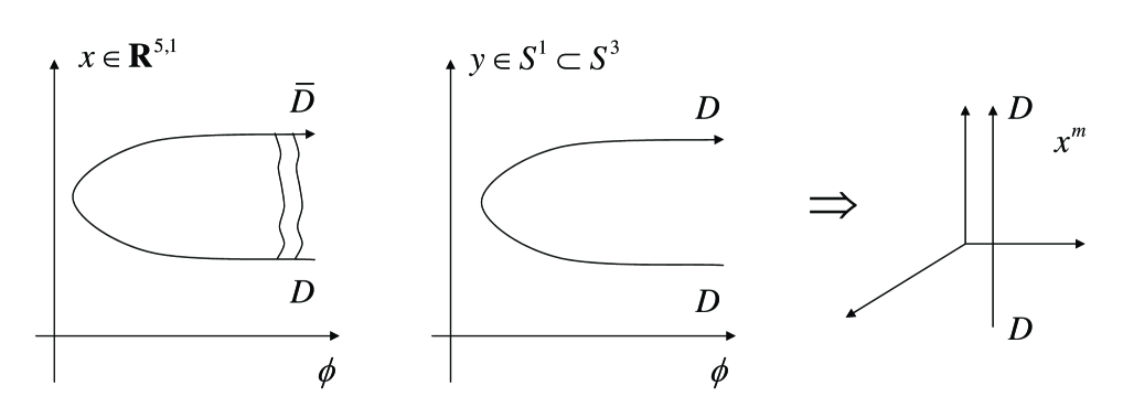
Figure 1: Hairpin curves in several directions

3 Rolling D-branes in NS5 Backgrounds

As we declared, we now attempt to make the Wick rotation of $X$ to the time coordinate $X^{0}$ in the non-BPS hairpin brane (2.17) to construct the boundary states describing the rolling D-brane solution (accompanied by the replacements $X\,\rightarrow\,X^{0}$, $\psi^{X}\,\rightarrow\,\psi^{X^{0}}$ in (2.35)). We again concentrate on the $P=Q=0$ case to avoid unessential complexities.

3.1 Wick Rotation to the Rolling D-brane

First of all, let us try to make the naive Wick rotation $q\rightarrow i\omega$ in (2.19), i.e.

$$\Psi^{(\mbox{\scriptsize NS})}_{\mbox{\scriptsize naive}}(p,\omega)=\sqrt{2}{\cal Q}e^{i\frac{2p}{{\cal Q}}\ln\tilde{r}}\frac{\Gamma(-i{\cal Q}p)\Gamma(1-i\frac{2p}{{\cal Q}})}{\Gamma(\frac{1}{2}+i\frac{\omega}{{\cal Q}}-i\frac{p}{{\cal Q}})\Gamma(\frac{1}{2}-i\frac{\omega}{{\cal Q}}-i\frac{p}{{\cal Q}})}~{},$$ (3.1)

where we introduced the parameter $\tilde{r}$ in (2.20) which will be identified as $\tilde{r}=\frac{2E}{\tau_{p}}$ in the rolling D-brane solution (1.1). Unfortunately this result is physically unacceptable because of the bad UV behavior. We cannot Fourier transform it and thus cannot reproduce the correct trajectory of the rolling D-brane solution (1.1). In fact, the absolute square of this wave function behaves as

$$|\Psi_{\mbox{\scriptsize naive}}^{(\mbox{\scriptsize NS})}(p,\omega)|^{2}\sim\frac{\cosh(\frac{2\pi\omega}{{\cal Q}})+\cosh(\frac{2\pi p}{{\cal Q}})}{\sinh(\pi{\cal Q}p)\sinh(\frac{2\pi p}{{\cal Q}})}~{},$$ (3.2)

which is divergent under $\omega\rightarrow\infty$.

On the other hand, the following wave function is physically acceptable, which is obtained via the Wick rotation in the position space $x\rightarrow it$;

$$\tilde{\Psi}^{(\mbox{\scriptsize NS})}(\phi,t)=\frac{\sqrt{2}}{\pi{{\cal Q}}\Big{(}2\cosh\frac{{\cal Q}t}{2}\Big{)}^{\frac{2}{{\cal Q}^{2}}+1}}\exp\Big{[}-\frac{\phi^{\prime}}{{\cal Q}}-\frac{e^{-\frac{\phi^{\prime}}{{\cal Q}}}}{\Big{(}2\cosh\frac{{\cal Q}t}{2}\Big{)}^{\frac{2}{{\cal Q}^{2}}}}\Big{]},\quad\phi^{\prime}\equiv\phi-\frac{2}{{\cal Q}}\ln\tilde{r}.$$ (3.3)

As is obvious from the construction, the peak of this wave function is located at the trajectory of the rolling D-brane (1.1). In addition this wave function vanishes as $|t|\rightarrow\infty$ due to the suppression factor $\sim 1/\cosh t$, as expected from the low energy analysis using the DBI action. It has a well-defined Fourier transform;

$$\begin{split}\Psi^{(\mbox{\scriptsize NS})}(p,\omega)&=\int_{-\infty}^{\infty}d\phi\int_{-\infty}^{\infty}dt\,e^{ip\phi}e^{-i\omega t}\tilde{\Psi}^{(\mbox{\scriptsize NS})}(\phi,t)\\ &=\frac{\sqrt{2}}{\pi}e^{\frac{2ip}{{\cal Q}}\ln\tilde{r}}\Gamma(1-i{\cal Q}p)\int_{-\infty}^{\infty}dt\,\Big{(}2\cosh\frac{{\cal Q}t}{2}\Big{)}^{-i\frac{2p}{{\cal Q}}-1}e^{-i\omega t}.\end{split}$$ (3.4)

In fact, the integral in the second line is manifestly convergent.

One might ask why the naive Wick-rotation leads to a wrong result. The answer is very simple: Due to the existence of Heaviside function the R.H.S. of the formula (2.23) is not analytic and we cannot analytically continue it.

Another natural question would be how we can reproduce the position space wave function (3.3) from the one in the momentum space. To answer the question we return to the wave function of hairpin brane (2.19). To simplify the arguments we eliminate ${\cal Q}$ by redefining the momenta and positions like $\frac{2p}{{\cal Q}}\rightarrow p$ and $\frac{{\cal Q}x}{2}\rightarrow x$. Again due to this Heaviside function, the contribution of the hairpin D-brane comes only from the region $-\pi/2<x<\pi/2$,

$$\int_{-\frac{\pi}{2}}^{\frac{\pi}{2}}dx\,(2\cos x)^{-ip-1}e^{iqx}=\frac{\pi\Gamma(-ip)}{\,\Gamma(\frac{1}{2}-\frac{q}{2}-i\frac{p}{2})\Gamma(\frac{1}{2}+\frac{q}{2}-i\frac{p}{2})}.$$ (3.5)

Then we need to extend the integration contour to an infinite line to make the Wick rotation possible with keeping the integral convergent. Note that the function $\ln\cos x$ has branch cuts between $-\frac{3\pi}{2}+2\pi m<x<-\frac{\pi}{2}+2\pi m$, ($m\in\mbox{{\bf Z}}$) on the real line. We so find that the contour should be set as in fig.2.

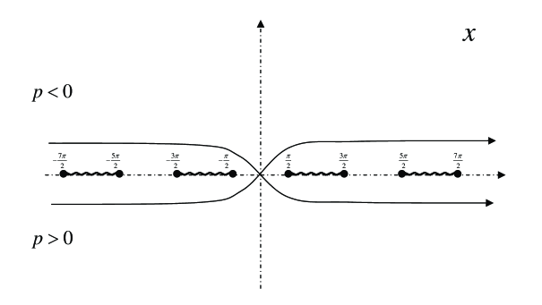
Figure 2: Branch cuts and contour

For $p>0$ the integral can be calculated as follows

$$\begin{split}&\int_{{\cal C}}dx\,[2\cos x]^{-ip-1}e^{iqx}\\ &=\lim_{\epsilon\to 0^{+}}\int_{-\infty}^{\frac{\pi}{2}}dx\,[2\cos(x-i\epsilon)]^{-ip-1}e^{iqx}+\lim_{\epsilon\to 0^{+}}\int_{\frac{\pi}{2}}^{\infty}dx\,[2\cos(x+i\epsilon)]^{-ip-1}e^{iqx}\\ &=\Big{[}\sum_{m=-\infty}^{0}(-e^{\pi p}e^{i\pi q})^{m}+\sum_{m=1}^{\infty}(-e^{-\pi p}e^{i\pi q})^{m}\Big{]}\int_{-\frac{\pi}{2}}^{\frac{\pi}{2}}dx\,(2\cos x)^{-ip-1}e^{iqx}\\ &=\Big{[}\frac{1}{1+e^{-\pi(p+iq)}}+\frac{1}{1+e^{-\pi(p-iq)}}-1\Big{]}\frac{\pi\Gamma(-ip)}{\Gamma(\frac{1}{2}-\frac{q}{2}-i\frac{p}{2})\Gamma(\frac{1}{2}+\frac{q}{2}-i\frac{p}{2})}.\end{split}$$ (3.6)

The third line in (3.6) takes the form of the summation over the contribution of each hairpin brane located in the interval $\frac{2m-1}{2}\pi<x<\frac{2m+1}{2}\pi$. We can likewise calculate for $p<0$ and the result is summarized as follows;

$$\begin{split}&\int_{{\cal C}}dx\,[2\cos x]^{-ip-1}e^{iqx}\\ &=\frac{\mbox{sgn}(p)\sinh(\pi p)}{2\cosh[\frac{\pi}{2}(p+iq)]\cosh[\frac{\pi}{2}(p-iq)]}\times\frac{\pi\Gamma(-ip)}{\Gamma(\frac{1}{2}-\frac{q}{2}-i\frac{p}{2})\Gamma(\frac{1}{2}+\frac{q}{2}-i\frac{p}{2})}.\end{split}$$ (3.7)

Note that the additional factor is an even function of $p$. Hence the derived wave function is compatible with the reflection relation in the ${\cal N}=2$ Liouville theory.

Now, for $-1<q<1$, we can Wick-rotate the contour ${\cal C}$ to the imaginary line $(x=it)$ with avoiding crossing the branch cuts;

$$\begin{split}&\int_{-i\infty}^{i\infty}dx\,[2\cos x]^{-ip-1}e^{iqx}=i\int_{-\infty}^{\infty}dt\,[2\cosh t]^{-ip-1}e^{-qt}\\ &=\frac{\sinh(\pi p)}{2\cosh[\frac{\pi}{2}(p+iq)]\cosh[\frac{\pi}{2}(p-iq)]}\frac{\pi\Gamma(-ip)}{\Gamma(\frac{1}{2}-\frac{q}{2}-i\frac{p}{2})\Gamma(\frac{1}{2}+\frac{q}{2}-i\frac{p}{2})}.\end{split}$$ (3.8)

Since both sides of (3.8) are clearly analytic with respect to $q$ around the imaginary line, the analytic continuation $q=i\omega$ can be performed. This continuation leads to

$$\begin{split}&\int_{-\infty}^{\infty}dt\,[2\cosh t]^{-ip-1}e^{-i\omega t}\\ &=\Big{[}\frac{1}{1+e^{-\pi(p+\omega)}}+\frac{1}{1+e^{-\pi(p-\omega)}}-1\Big{]}\times\frac{-i\pi\Gamma(-ip)}{\Gamma[\frac{1}{2}-\frac{i}{2}(p-\omega)]\Gamma[\frac{1}{2}-\frac{i}{2}(p+\omega)]}\\ &=\frac{\sinh(\pi p)}{2\cosh[\frac{\pi}{2}(p+\omega)]\cosh[\frac{\pi}{2}(p-\omega)]}\times\frac{-i\pi\Gamma(-ip)}{\Gamma[\frac{1}{2}-\frac{i}{2}(p-\omega)]\Gamma[\frac{1}{2}-\frac{i}{2}(p+\omega)]}.\end{split}$$ (3.9)

It is remarkable that we now have an additional suppression factor which improves the UV behavior of $\omega$. This is quite reminiscent of the one characteristic for the rolling tachyon solution (full s-brane) [1].

Finally, after restoring ${\cal Q}$, we find that the rolling D-brane can be expressed in the momentum space as follows;

$$\Psi^{(\mbox{\scriptsize NS})}(p,\omega) = \frac{-i\sinh(\frac{2\pi p}{{\cal Q}})}{2\cosh[\frac{\pi}{{\cal Q}}(p+\omega)]\cosh[\frac{\pi}{{\cal Q}}(p-\omega)]}\,\Psi^{(\mbox{\scriptsize NS})}_{\mbox{\scriptsize naive}}(p,\omega)$$ (3.10)

$$= \frac{-i\sqrt{2}{\cal Q}e^{i\frac{2p}{{\cal Q}}\ln\tilde{r}}\sinh(\frac{2\pi p}{{\cal Q}})}{2\cosh[\frac{\pi}{{\cal Q}}(p+\omega)]\cosh[\frac{\pi}{{\cal Q}}(p-\omega)]}\cdot\frac{\Gamma(-i{\cal Q}p)\Gamma(1-i\frac{2p}{{\cal Q}})}{\Gamma(\frac{1}{2}+i\frac{\omega}{{\cal Q}}-i\frac{p}{{\cal Q}})\Gamma(\frac{1}{2}-i\frac{\omega}{{\cal Q}}-i\frac{p}{{\cal Q}})}.$$

Its absolute square is

$$|\Psi^{(\mbox{\scriptsize NS})}(p,\omega)|^{2}=\frac{2\sinh\left(\frac{2\pi p}{{\cal Q}}\right)}{\left[\cosh\left(\frac{2\pi\omega}{{\cal Q}}\right)+\cosh\left(\frac{2\pi p}{{\cal Q}}\right)\right]\sinh(\pi{\cal Q}p)}\ .$$ (3.11)

In the R sector the Wick rotation becomes a little bit different. If we substitute $q=i\omega$ into the R wave function after the Wick rotation as we have just done, we obtain

$$\Psi^{(\mbox{\scriptsize R})}(p,\omega)=\frac{-i\sqrt{2}{\cal Q}e^{i\frac{2p}{{\cal Q}}\ln\tilde{r}}\sinh\left(\frac{2\pi p}{{\cal Q}}\right)}{\cosh\left(\frac{2\pi p}{{\cal Q}}\right)-\cosh\left(\frac{2\pi\omega}{{\cal Q}}\right)}\cdot\frac{\Gamma(-i{\cal Q}p)\Gamma\left(1-i\frac{2p}{{\cal Q}}\right)}{\Gamma\left(1-i\frac{p}{{\cal Q}}-i\frac{\omega}{{\cal Q}}\right)\Gamma\left(-i\frac{p}{{\cal Q}}+i\frac{\omega}{{\cal Q}}\right)}\ .$$ (3.12)

One of the easiest way to obtain this result is to substitute $\omega_{\mbox{\scriptsize NS}}=\omega_{\mbox{\scriptsize R}}-\frac{i{\cal Q}}{2}$ into the NS wave function (3.10). Its absolute square is given by

$$|\Psi^{(\mbox{\scriptsize R})}(p,\omega)|^{2}=\frac{\omega-p}{\omega+p}\frac{2\sinh\left(\frac{2\pi p}{{\cal Q}}\right)}{\left[\cosh\left(\frac{2\pi\omega}{{\cal Q}}\right)-\cosh\left(\frac{2\pi p}{{\cal Q}}\right)\right]\sinh(\pi{\cal Q}p)}\ .$$ (3.13)

The subtlety here is that we no longer have a sensible GSO projection for the open sector. Recalling the symmetry with respect to $p$ and $-p$, we can rewrite this in a more suggestive form

$$|\Psi^{(\mbox{\scriptsize R})}(p,\omega)|^{2}=\frac{\omega^{2}+p^{2}}{(\omega^{2}-p^{2})}\frac{2\sinh\left(\frac{2\pi p}{{\cal Q}}\right)}{\left[\cosh\left(\frac{2\pi\omega}{{\cal Q}}\right)-\cosh\left(\frac{2\pi p}{{\cal Q}}\right)\right]\sinh(\pi{\cal Q}p)}\ .$$ (3.14)

It is interesting to observe that the R sector has a singularity when $p=\pm\omega$ i.e. in the case of the massless forward (and backward) emission from the rolling D-brane.

Several comments are in order:

1. The “time-like ${\cal N}=2$ Liouville theory” we are considering here is defined only by the Wick rotation of $X$ with leaving $\phi$ space-like, and not accompanied by the analytic continuation of any parameter in the model (say, the background charge ${\cal Q}$). This point is in a sharp contrast with the bosonic time-like Liouville theory [28, 29, 30], in which the time-like $\phi$ is considered and also the analytic continuation of the parameter is taken.

2. As we already addressed, the boundary wave function (3.10) for the rolling D-brane we proposed includes a suppression factor for energy $\omega$, which improves the UV behavior and reproduces the correct profile of rolling brane. Although this seems quite satisfactory, a subtlety now appears since this factor is an odd function of $p$. One may be afraid that it would contradict the reflection amplitude in the Liouville theory. However, it originates from the Wick rotation, namely, the factor $\mbox{sgn}(p)$ in eq.(3.7) is canceled by the orientation of the Wick-rotated contour. We again stress that our boundary wave function is originally consistent with the reflection amplitude before performing the Wick rotation (recall (3.7)), and thus should be the correct one according to the spirit of Wick rotation. It may be interesting to further investigate whether such peculiarity is a general feature in the time-like ${\cal N}=2$ Liouville theory.

3. The prefactor discussed above has the similar form to that for the rolling tachyon solution, as already mentioned. This fact reminds us of the interpretation of the rolling tachyon solution (with a certain coupling constant) as an array of the sD-branes on the imaginary time axis discussed in [1, 31, 32, 33]. It may be fascinating to ask whether the similar interpretation is possible for the rolling D-brane: the interpretation as an array of the infinite hairpin branes along the imaginary axis.

4. Another natural question is whether the rolling brane boundary state (3.10) really satisfies the Cardy condition. It is not so difficult to confirm this is indeed the case among the rolling branes themselves, as well as with arbitrary static branes that are trivial along the $\phi$, $X^{0}$-directions. However, if we consider the branes associated to degenerate representations in the time-like ${\cal N}=2$ Liouville theory here, the situation gets quite subtle. For example, one might consider the “time-dependent class 1 brane” (ZZ-type) associated to the identity representation [13, 14]. The overlap with it should satisfy the modular bootstrap equation. Unfortunately, it does not seem to be the case, since the prefactor considered here is not likely to be identified as a modular coefficient of any unitary representation of ${\cal N}=2$ SCA. However, we here note that the time-like characters of degenerate representations cannot completely cancel the contributions from the ghost oscillators due to the existence of singular vectors. From this fact, one can easily find that any time-dependent brane of a degenerate representation always include negative norm states in the open channel, even if it is a unitary representation. Hence, it is plausible to discard such time-dependent “degenerate” branes, and in this sense, our rolling brane (3.10) does not contradict the Cardy condition. Further studies would be needed for this issue.

3.2 Open String Density of States and Closed String Emission

By using the boundary wave functions we obtained (3.10), (3.12), we can evaluate the open channel density of states and the closed string emission rate in the rolling process. The density of states in the open channel is calculated in the same way as the previous analysis

$$\rho^{(\mbox{\scriptsize NS})}(p^{\prime},\omega^{\prime}) = \int_{-\infty}^{\infty}d\omega\int_{0}^{\infty}dp\,2\cos(2\pi pp^{\prime})\cos(2\pi\omega\omega^{\prime})\frac{2\sinh\left(\frac{2\pi p}{{\cal Q}}\right)}{\left[\cosh\left(\frac{2\pi\omega}{{\cal Q}}\right)+\cosh\left(\frac{2\pi p}{{\cal Q}}\right)\right]\sinh(\pi{\cal Q}p)}$$ (3.15)

$$= \frac{2\sinh\left(\frac{2\pi\omega^{\prime}}{{\cal Q}}\right)}{\left[\cosh\left(\frac{2\pi\omega^{\prime}}{{\cal Q}}\right)+\cosh\left(\frac{2\pi p^{\prime}}{{\cal Q}}\right)\right]\sinh(\pi{\cal Q}\omega^{\prime})}\ ,$$ (3.16)

for the NS sector by using the Fourier transformation formula;

$$\int_{-\infty}^{\infty}\frac{dk}{2\pi}\frac{\sinh(a\pi)}{\cosh(k)+\cosh(a\pi)}e^{ikx}=\frac{\sin(a\pi x)}{\sinh(\pi x)}\ .$$ (3.17)

It is amazing that the result is simply given by the exchange of momentum and energy of the closed channel amplitudes. This self-dual property of the amplitudes is peculiar to this function. At the same time, the result shows that our open channel density is manifestly positive definite as it should be.

On the other hand, for the R sector or the open $\widetilde{\mbox{NS}}$ sector equivalently, the density of states has a divergence on the light-cone direction $\omega=\pm p$.

$$\rho^{(\widetilde{\mbox{\scriptsize NS}})}(p^{\prime},\omega^{\prime})=\int_{-\infty}^{\infty}d\omega\int_{0}^{\infty}dp\,2\cos(2\pi pp^{\prime})\cos(2\pi\omega\omega^{\prime})$$

$$\hskip 85.35826pt\times\frac{\omega^{2}+p^{2}}{(\omega^{2}-p^{2})}\frac{2\sinh\left(\frac{2\pi p}{{\cal Q}}\right)}{\left[\cosh\left(\frac{2\pi\omega}{{\cal Q}}\right)-\cosh\left(\frac{2\pi p}{{\cal Q}}\right)\right]\sinh(\pi{\cal Q}p)}\ .$$ (3.18)

This divergence comes from the double pole of the absolute square of the boundary wave function, which is typical of the infrared divergence for the extending branes in the Liouville theories (FZZT-like branes). This fact suggests that our brane is extending along a non-compact direction and reaches the speed of light in the far past and future, as is expected. The reason why the NS amplitude, in contrast, does not have such a divergence is intuitively understood as follows: In the CHS background the string coupling tends to be stronger and stronger as the brane comes close to the NS5-brane. As a result, the tension of the brane gets smaller in the far past and future, and thus the gravitational interaction practically vanishes. On the other hand, the RR scattering does not damp because the coupling to the RR field does not depend on the value of the dilaton. Hence, in view of the RR field probe, the rolling brane is actually extending from the past to the future.

The difference between the density of states in the open NS and $\widetilde{\mbox{NS}}$ sector obviously shows that our rolling brane is not supersymmetric nor GSO projected, as is expected since we started from the non-BPS hairpin brane (2.19).

Now let us calculate the closed string emission rate. We again begin with the NS sector. Analysing the self-overlap and using the optical theorem, the emission rate for a fixed transverse mass $M$ is evaluated in the similar manner to [32, 34] as

$$\bar{N}^{(\mbox{\scriptsize NS})}(M)=\int_{0}^{\infty}\frac{dp}{\omega_{p}}\,\frac{2\sinh\left(\frac{2\pi p}{{\cal Q}}\right)}{\left[\cosh\left(\frac{2\pi\omega_{p}}{{\cal Q}}\right)+\cosh\left(\frac{2\pi p}{{\cal Q}}\right)\right]\sinh(\pi{\cal Q}p)}\ ,\ \omega_{p}=\sqrt{p^{2}+M^{2}}\ .$$ (3.19)

It is convergent if $M^{2}>0$. On the other hand, for the R sector, the emission rate is given by

$$\bar{N}^{(\mbox{\scriptsize R})}(M)=\int_{0}^{\infty}\frac{dp}{\omega_{p}}\,\frac{\omega_{p}^{2}+p^{2}}{(\omega_{p}^{2}-p^{2})}\frac{2\sinh\left(\frac{2\pi p}{{\cal Q}}\right)}{\left[\cosh\left(\frac{2\pi\omega_{p}}{{\cal Q}}\right)-\cosh\left(\frac{2\pi p}{{\cal Q}}\right)\right]\sinh(\pi{\cal Q}p)}\ ,\ \omega_{p}=\sqrt{p^{2}+M^{2}}\ .$$ (3.20)

This emission rate has a strong peak at the massless forward scattering $M=0,p=\omega$, but otherwise it is convergent.

Let us evaluate the asymptotic behaviors of these emission rates in the large $M$ limit. It is obvious that $\bar{N}^{(\mbox{\scriptsize NS})}(M)$ and $\bar{N}^{(\mbox{\scriptsize R})}(M)$ have the same asymptotic behaviors. We consider D$p$-brane, which has $d=5-p$ transverse directions to the D-brane in $\mbox{{\bf R}}^{5}$. Then the asymptotic emission rate behaves as

$$\bar{N}(M)\sim\int d^{d}k_{\perp}\int_{0}^{\infty}\frac{dp}{M}\,e^{\left(\frac{2\pi}{{\cal Q}}-\pi{\cal Q}\right)p-\frac{2\pi}{{\cal Q}}\sqrt{p^{2}+k^{2}_{\perp}+M^{2}}}\sim M^{\frac{-1+d}{2}}e^{-2\pi M\sqrt{1-\frac{{\cal Q}^{2}}{4}}}~{},$$ (3.21)

where we used the saddle point approximation. The density of levels as a function of mass, however, is given by $n(M)\propto M^{-3}e^{2\pi M\sqrt{1-\frac{{\cal Q}^{2}}{4}}}$, which is obtained by recalling $c_{\mbox{\scriptsize eff}}=12-3{\cal Q}^{2}$ because of the linear dilaton background [35]. Thus, the total emission rate becomes

$$\frac{\bar{N}}{V}\sim\int^{\infty}dM\,M^{-\frac{p}{2}-1}~{},~{}~{}~{}\frac{\bar{E}}{V}\sim\int^{\infty}dM\,M^{-\frac{p}{2}}\ .$$ (3.22)

The total emitted energy has a powerlike divergence when $p\leq 2$. This fact contrasts with the UV finite brane decay in the bosonic linear dilaton background studied in [34], and rather leads us to the same behavior as the decay of the non-BPS brane in the flat Minkowski space [32].

In this subsection we have discussed only the one closed string emission from the rolling brane. Owing to this limitation the rate of emission to the tangential direction to the brane vanishes simply by the momentum conservation. In the processes of two or more string emissions, the amplitudes for the tangential emissions could be non-zero. However, from the experience in the two-dimensional string theories (see, e.g. [37, 38, 39, 40, 41]), we believe that the inclusion of these decaying modes does not improve the qualitative properties of the worldsheet analysis. The quantum treatment of the D-brane should be necessary in order to truly understand the fate of rolling D-brane.

4 Summary and Discussions

In this paper we studied a solution of time-dependent D-branes, the rolling D-branes, in the NS5 background by means of the BCFT approach. An interesting point addressed in [10] is that the rolling D-brane has similarities to the rolling tachyon, which suggests that the BCFT analysis is helpful for further studies. With this motivation, we have constructed the boundary state for the rolling D-brane. The Wick-rotated version of the rolling D-brane is a hairpin brane whose boundary state has been constructed in the bosonic theory in [11]. We can supersymmetrize the hairpin D-brane as the class 2 (FZZT) D-brane in ${\cal N}=2$ Liouville theory [13, 14]. This is quite natural because ${\cal N}=2$ Liouville theory is regarded as a supersymmetric extension of the sine-Liouville theory where the bosonic hairpin brane is considered in [11].

These hairpin D-branes can be embedded in the CHS background in two ways. When the direction of ${\cal N}=2$ $U(1)$-current is set to be in the internal direction, i.e. $S^{1}$ in $S^{3}$, the hairpin D-brane is a BPS one. We confirmed this fact by analysing explicitly the self-overlap of boundary states. On the other hand, when we choose the $U(1)$-direction parallel to NS5 (and decompactify it), the hairpin D-brane breaks all supersymmetries. In this case we found the non-vanishing self-overlap which suggests that the two sides of hairpin looks like a $D\bar{D}$-system in the asymptotic region. Moreover, this is a stable non-BPS brane. This fact is physically understood as follows: The Liouville interaction prevents the $D\bar{D}$ open strings from shrinking to the corner of the hairpin and the mass square of the tachyon modes actually gets positive.

As the highlight of this work, we have proposed an appropriate way of the Wick rotation to the rolling D-brane. By performing the Wick rotation in the position space, we have arrived at a sensible boundary wave function that provides well-defined spectral densities of open string states. Furthermore, it successfully reproduces the correct trajectory of rolling D-brane under the classical limit. It is remarkable that our procedure of Wick rotation gives rise to the prefactor quite analogous to that for the rolling tachyon solution [1], which improves the UV behavior of the boundary wave function . This fact is likely to support the similarity to the rolling tachyon recognized by Kutasov. This prefactor could be interpreted to originate from an infinite array of the Euclidean hairpin branes in the similar manner as the rolling tachyon case [1, 31, 32, 33]. We also calculated the closed string emission rate in both the NS and R sectors. The different behaviors of emission rates between the NS and R sectors have been found and explained from the physical viewpoints.

We can easily extend our results to other non-trivial backgrounds, say, non-compact Calabi-Yau 3-folds, just by replacing the ${\cal N}=2$ minimal sector with other solvable superconformal models. The dual gauge theory or the LST interpretations of our results and their extension to various setups may be also interesting subjects which deserves further studies. It will be also important to extend our results to the rolling D-branes with non-vanishing angular momentum in $S^{3}$, which are also discussed in [10]. Recalling we can get the trajectory only by rescaling the time direction, we may construct the boundary states for these D-branes only by adding a factor in front of the energy $\omega$ in the wave functions with some proper combinations of the Ishibashi states of $SU(2)$.

To conclude the whole paper, let us comment on the possible fate of the rolling D-brane. As we can see from the boundary states (or classical analysis), the rolling brane inevitably approaches the strong coupling region in the far past and future unlike the hairpin brane. This has a physical interpretation: It loses all the energy and eventually gets absorbed into the NS5-branes, making a bound state as was discussed in [10]. To capture this nonperturbative physics is beyond the scope of boundary state analysis. One possible approach to this problem may be to lift the whole setup to the M-theory (see [6] in the context of LST). Indeed, taking into consideration the success of M-theoretic approach to the nonperturbative physics involving the static NS5-brane and D-branes (e.g. Hanany-Witten setup), we expect this will be an interesting future direction worth pursuing.

Appendix A   Note on ${\cal N}=2$ Minimal Characters

A simple way to realize the level $k$ ${\cal N}=2$ minimal model $(\hat{c}=k/(k+2))$ is to use the Kazama-Suzuki coset $\frac{SU(2)_{k}\times U(1)_{2}}{U(1)_{k+2}}$. We then have the following branching relation;

$$\chi_{\ell}^{(k)}(\tau,w)\Theta_{s,2}(\tau,w-z)=\sum_{\stackrel{{\scriptstyle m\in\mbox{\scriptsize{\bf Z}}_{2(k+2)}}}{{\ell+m+s\in 2\mbox{\scriptsize{\bf Z}}}}}\chi_{m}^{\ell,s}(\tau,z)\Theta_{m,k+2}(\tau,w-2z/(k+2))~{},$$

$$\chi^{\ell,s}_{m}(\tau,z)\equiv 0~{},~{}~{}~{}\mbox{for $\ell+m+s\in 2\mbox{{\bf Z}}+1$}~{},$$ (A.1)

where $\chi_{\ell}^{(k)}(\tau,z)$ is the spin $\ell/2$ character of $SU(2)_{k}$;

$$\chi^{(k)}_{\ell}(\tau,z)=\frac{\Theta_{\ell+1,k+2}(\tau,z)-\Theta_{-\ell-1,k+2}(\tau,z)}{\Theta_{1,2}(\tau,z)-\Theta_{-1,2}(\tau,z)}\equiv\sum_{m\in\mbox{\scriptsize{\bf Z}}_{2k}}\,c^{(k)}_{\ell,m}(\tau)\Theta_{m,k}(\tau,z)~{}.$$ (A.2)

The branching function $\chi^{\ell,s}_{m}(\tau,z)$ is explicitly calculated as follows ;

$$\chi_{m}^{\ell,s}(\tau,z)=\sum_{r\in\mbox{\scriptsize{\bf Z}}_{k}}c^{(k)}_{\ell,m-s+4r}(\tau)\Theta_{2m+(k+2)(-s+4r),2k(k+2)}(\tau,z/(k+2))~{}.$$ (A.3)

Then, the character formulae of unitary representations are written as

$$\mbox{ch}^{(\mbox{\scriptsize NS})}_{\ell,m}(\tau,z)=\chi^{\ell,0}_{m}(\tau,z)+\chi^{\ell,2}_{m}(\tau,z)~{},$$

$$\mbox{ch}^{(\widetilde{\mbox{\scriptsize NS}})}_{\ell,m}(\tau,z)=\chi^{\ell,0}_{m}(\tau,z)-\chi^{\ell,2}_{m}(\tau,z)\equiv e^{-i\pi\frac{m}{k+2}}\mbox{ch}^{(\mbox{\scriptsize NS})}_{\ell,m}\left(\tau,z+\frac{1}{2}\right)~{},$$

$$\mbox{ch}^{(\mbox{\scriptsize R})}_{\ell,m}(\tau,z)=\chi^{\ell,1}_{m}(\tau,z)+\chi^{\ell,3}_{m}(\tau,z)\equiv q^{\frac{k}{8(k+2)}}y^{\frac{k}{2(k+2)}}\mbox{ch}^{(\mbox{\scriptsize NS})}_{\ell,m+1}\left(\tau,z+\frac{\tau}{2}\right)~{},$$

$$\mbox{ch}^{(\widetilde{\mbox{\scriptsize R}})}_{\ell,m}(\tau,z)=\chi^{\ell,1}_{m}(\tau,z)-\chi^{\ell,3}_{m}(\tau,z)\equiv-e^{-i\pi\frac{m+1}{k+2}}q^{\frac{k}{8(k+2)}}y^{\frac{k}{2(k+2)}}\mbox{ch}^{(\mbox{\scriptsize NS})}_{\ell,m+1}\left(\tau,z+\frac{1}{2}+\frac{\tau}{2}\right)~{}.$$

(A.4)

By definition, we may restrict to $\ell+m\in 2\mbox{{\bf Z}}$ for the NS and $\widetilde{\mbox{NS}}$ sectors, and to $\ell+m\in 2\mbox{{\bf Z}}+1$ for the R and $\widetilde{\mbox{R}}$ sectors. It is convenient to define $\mbox{ch}^{(\sigma)}_{*}(\tau,z)\equiv 0$ unless these conditions for $\ell$, $m$ are satisfied. Note the character identity (“field identification”)

$$\chi^{k-\ell,s+2}_{m+k+2}(\tau,z)=\chi^{\ell,s}_{m}(\tau,z)~{},$$ (A.5)

or equivalently,

$$\mbox{ch}^{(\sigma)}_{k-\ell,m+k+2}(\tau,z)=\mbox{ch}^{(\sigma)}_{\ell,m}(\tau,z)~{},~{}~{}(\sigma=\mbox{NS},\,\mbox{R})~{},$$

$$\mbox{ch}^{(\sigma)}_{k-\ell,m+k+2}(\tau,z)=-\mbox{ch}^{(\sigma)}_{\ell,m}(\tau,z)~{},~{}~{}(\sigma=\widetilde{\mbox{NS}},\,\widetilde{\mbox{R}})~{}.$$ (A.6)

References

- [1] A. Sen, JHEP 0204, 048 (2002) [arXiv:hep-th/0203211]; JHEP 0207, 065 (2002) [arXiv:hep-th/0203265]; Mod. Phys. Lett. A 17, 1797 (2002) [arXiv:hep-th/0204143].
- [2] M. Gutperle and A. Strominger, JHEP 0204, 018 (2002) [arXiv:hep-th/0202210].
- [3] A. Strominger, arXiv:hep-th/0209090.
- [4] C. G. . Callan, J. A. Harvey and A. Strominger, arXiv:hep-th/9112030.
- [5] H. Ooguri and C. Vafa, Nucl. Phys. B 463, 55 (1996) [arXiv:hep-th/9511164].
- [6] O. Aharony, M. Berkooz, D. Kutasov and N. Seiberg, JHEP 9810, 004 (1998) [arXiv:hep-th/9808149].
- [7] A. Giveon, D. Kutasov and O. Pelc, JHEP 9910, 035 (1999) [arXiv:hep-th/9907178].
- [8] A. Giveon and D. Kutasov, JHEP 9910, 034 (1999) [arXiv:hep-th/9909110]; A. Giveon and D. Kutasov, JHEP 0001, 023 (2000) [arXiv:hep-th/9911039].
- [9] Y. Nakayama, arXiv:hep-th/0402009.
- [10] D. Kutasov, arXiv:hep-th/0405058.
- [11] S. L. Lukyanov, E. S. Vitchev and A. B. Zamolodchikov, Nucl. Phys. B 683, 423 (2004) [arXiv:hep-th/0312168].
- [12] S. Ribault and V. Schomerus, JHEP 0402, 019 (2004) [arXiv:hep-th/0310024].
- [13] T. Eguchi and Y. Sugawara, JHEP 0401, 025 (2004) [arXiv:hep-th/0311141].
- [14] C. Ahn, M. Stanishkov and M. Yamamoto, Nucl. Phys. B 683, 177 (2004) [arXiv:hep-th/0311169].
- [15] J. McGreevy, S. Murthy and H. Verlinde, JHEP 0404, 015 (2004) [arXiv:hep-th/0308105].
- [16] D. Israel, A. Pakman and J. Troost, arXiv:hep-th/0405259.
- [17] C. Ahn, M. Stanishkov and M. Yamamoto, arXiv:hep-th/0405274.
- [18] A. Fotopoulos, V. Niarchos and N. Prezas, arXiv:hep-th/0406017.
- [19] V. Fateev, A. B. Zamolodchikov and A. B. Zamolodchikov, arXiv:hep-th/0001012; J. Teschner, arXiv:hep-th/0009138.
- [20] A. Recknagel and V. Schomerus, Nucl. Phys. B 531, 185 (1998) [arXiv:hep-th/9712186].
- [21] Y. Hikida, M. Nozaki and Y. Sugawara, Nucl. Phys. B 617, 117 (2001) [arXiv:hep-th/0101211].
- [22] J. L. Cardy, Nucl. Phys. B 324, 581 (1989).
- [23] A. Y. Alekseev, A. Recknagel and V. Schomerus, JHEP 9909, 023 (1999) [arXiv:hep-th/9908040].
- [24] C. Bachas, M. R. Douglas and C. Schweigert, JHEP 0005, 048 (2000) [arXiv:hep-th/0003037]; J. Pawelczyk, JHEP 0008, 006 (2000) [arXiv:hep-th/0003057].
- [25] A. Sen, arXiv:hep-th/9904207.
- [26] P. Baseilhac and V. A. Fateev, Nucl. Phys. B 532, 567 (1998) [arXiv:hep-th/9906010].
- [27] C. Ahn, C. Kim, C. Rim and M. Stanishkov, Phys. Rev. D 69, 106011 (2004) [arXiv:hep-th/0210208].
- [28] M. Gutperle and A. Strominger, Phys. Rev. D 67, 126002 (2003) [arXiv:hep-th/0301038].
- [29] A. Strominger and T. Takayanagi, Adv. Theor. Math. Phys. 7, 2 (2003) [arXiv:hep-th/0303221].
- [30] V. Schomerus, JHEP 0311, 043 (2003) [arXiv:hep-th/0306026].
- [31] A. Maloney, A. Strominger and X. Yin, JHEP 0310, 048 (2003) [arXiv:hep-th/0302146].
- [32] N. Lambert, H. Liu and J. Maldacena, arXiv:hep-th/0303139.
- [33] D. Gaiotto, N. Itzhaki and L. Rastelli, Nucl. Phys. B 688, 70 (2004) [arXiv:hep-th/0304192].
- [34] J. L. Karczmarek, H. Liu, J. Maldacena and A. Strominger, JHEP 0311, 042 (2003) [arXiv:hep-th/0306132].
- [35] D. Kutasov and N. Seiberg, Nucl. Phys. B 358, 600 (1991).
- [36] D. A. Sahakyan, arXiv:hep-th/0408070.
- [37] J. McGreevy and H. Verlinde, JHEP 0312, 054 (2003) [arXiv:hep-th/0304224]; J. McGreevy, J. Teschner and H. Verlinde, JHEP 0401, 039 (2004) [arXiv:hep-th/0305194].
- [38] I. R. Klebanov, J. Maldacena and N. Seiberg, JHEP 0307, 045 (2003) [arXiv:hep-th/0305159].
- [39] T. Takayanagi and N. Toumbas, JHEP 0307, 064 (2003) [arXiv:hep-th/0307083].
- [40] M. R. Douglas, I. R. Klebanov, D. Kutasov, J. Maldacena, E. Martinec and N. Seiberg, arXiv:hep-th/0307195.
- [41] M. Gutperle and P. Kraus, Phys. Rev. D 69, 066005 (2004) [arXiv:hep-th/0308047].
- [42] V. Balasubramanian, E. Keski-Vakkuri, P. Kraus and A. Naqvi, arXiv:hep-th/0404039.