Twistor-Space Recursive Formulation of Gauge-Theory Amplitudes

Abstract

Using twistor space intuition, Cachazo, Svrcek and Witten presented novel diagrammatic rules for gauge-theory amplitudes, expressed in terms of maximally helicity-violating (MHV) vertices. We define non-MHV vertices, and show how to use them to give a recursive construction of these amplitudes. We also use them to illustrate the equivalence of various twistor-space prescriptions, and to determine the associated combinatoric factors.

I Introduction

In a striking recent paper WittenTopologicalString , Witten suggested that tree-level amplitudes of non-Abelian gauge theories can be obtained by integrating over the moduli space of certain $D$-instantons in the open-string topological B-model on (super) twistor space $\mathbb{CP}^{3|4}$. This proposal generalizes Nair’s earlier construction Nair of maximally helicity-violating amplitudes. It is a very promising step towards understanding why amplitudes in unbroken gauge theories are so much simpler than suggested by individual Feynman diagrams.

The best-known example of amplitudes with a remarkably simple structure are the Parke–Taylor amplitudes ParkeTaylor of QCD. These are amplitudes with two negative-helicity gluons and an arbitrary number of positive-helicity ones (or their parity conjugates), the so-called maximally helicity-violating (MHV) amplitudes. Inspired by the twistor-space structure underlying gauge-theory amplitudes in Witten’s proposal, Cachazo, Svrcek, and Witten (CSW) CSW have proposed a novel way to use off-shell continuations of MHV amplitudes to construct arbitrary tree-level amplitudes. This construction makes manifest the factorization on multi-particle poles. Although no-one has yet given a direct derivation of the CSW construction from a Lagrangian, the combination of the correct pole structure — that is, tree-level unitarity — and Lorentz invariance leaves little doubt that it is correct. It is worth noting that supersymmetry does not appear to play a special role in this construction, which is therefore valid in any gauge theory, including QCD Khoze .

In the original twistor-space formulation WittenTopologicalString , one obtains tree-level amplitudes with $d+1$ negative-helicity gluons from D-instantons of degree $d$. These might include both lone- and multi-instanton contributions, where the total degree of the instantons is $d$, and disconnected instantons are joined by twistor-space propagators.

In a series of papers Roiban, Spradlin, and Volovich RSV1 ; RSV2 computed the integrals over the moduli space of connected curves of degree $d$ and found that for $\overline{\rm MHV}$ amplitudes ($n$-point amplitudes with $n-2$ negative helicities, that is the parity conjugates of MHV, also called ‘googly-MHV’) and next-to-MHV amplitudes (with three negative helicities) this integral does reproduce the gauge theory amplitude. Since the integral over degree-$d$ curves gives the full result, it appears that one can ignore disconnected instantons. On the other hand, the CSW construction of gauge theory amplitudes is based on integrating over the moduli space of completely disconnected instantons of degree one, linked by twistor space propagators. Indeed, degree-one instantons correspond to MHV vertices; obtaining amplitudes with an arbitrary number of negative helicities using MHV vertices is dual in twistor space to integrating over degree-one instantons. We therefore seem to have different ways of computing the amplitudes from the topological B model.

In order to reconcile the two different computations, Gukov, Motl, and Neitzke Gukov examined the twistor space integrals over the moduli spaces of one degree-$d$ instanton and of $d$ degree-one instantons respectively. They argued that the former integral reduces to one on a special locus, where the degree $d$ curve degenerates into $d$ intersecting degree one curves. Similarly, the latter integral can be argued to reduce to one over the locus where the propagators have shrunk to zero size, which is also the place where the $d$ degree one curves intersect. Accordingly, it seems clear that the two prescriptions give the same result.

Following an analysis of degenerating twistor space curves, Gukov et. al. also suggested a set of ‘intermediate’ prescriptions for the amplitudes, in which one integrates over the moduli space of $k$ curves of degrees $d_{i}$ such that $\sum_{i=1}^{k}d_{i}=d$. In the extreme cases, $k=1$ and $k=d$, this reproduces the maximally connected and maximally disconnected calculations. They proposed that the amplitudes should be constructible from non-MHV vertices, though their form was not determined.

In this paper, we construct non-MHV vertices explicitly and use them to formulate intermediate prescriptions for tree-level amplitudes. Gukov et. al. Gukov used properties of curves in twistor space to investigate properties of amplitudes. Here we employ the connection in the opposite direction, using properties of amplitudes to determine the combinations of twistor-space curves that yield valid representations of the amplitudes. A simple approach to finding appropriate combinations of twistor-space curves that reproduce the gauge-theory amplitudes makes use of skeleton diagrams, which are like CSW diagrams, but stripped of their external legs. The set of twistor-space prescriptions corresponds to the possible reorganizations of MHV skeleton diagrams into diagrams including non-MHV vertices as well.

We also use the non-MHV vertices to formulate the CSW construction in a recursive fashion. Recursive methods have proven very powerful in QCD. Berends and Giele Recurrence used recurrence relations to give a proof of the Parke–Taylor equations ParkeTaylor , and later to derive explicit expressions WFourJet for processes such as $W+4$ jet production, the dominant background to top-quark production. These methods can be used both analytically and numerically. Beyond MHV amplitudes, they have also been used to obtain an all-$n$ form for the adjacent three-negative-helicity amplitude LightConeRecurrence . For this same class of amplitudes, CSW presented a remarkably simple derivation of an explicit formula for the amplitude. Their construction of course allows one to compute any amplitude; but as the number of negative-helicity legs increases, the number of diagrams and hence the computational complexity still increases exponentially RSV2 . Just as in the older case of Feynman diagrams, recursive methods can reduce this computational complexity. The recursive expressions we present in this paper can likewise be used directly for numerical computations as well as analytic ones. We will focus on amplitudes with external gluons, but our formulæ generalize in a straightforward way to amplitudes with external fermions or scalars Khoze , in both supersymmetric and nonsupersymmetric theories.

Alternative approaches to using string theories to compute gauge theory amplitudes have appeared in ref. Berkovits ; Vafa ; Siegel . Also, the twistor-space formulation breaks manifest parity relations, such as between MHV and $\overline{\rm MHV}$ amplitudes WittenTopologicalString ; RSV1 ; OtherGoogly , but it has been shown to hold generally for twistor-space amplitudes BerkovitsMotl ; RSV2 ; WittenParity .

What about loop amplitudes? Recently, Berkovits and Witten have noted BerkovitsWitten that the field theory described by the topological B-model in $\mathbb{CP}^{3|4}$, or alternatively by the open string theory proposed in refs. Berkovits ; BerkovitsMotl , is not pure ${\cal{N}}=4$ super-Yang Mills theory, but rather super-Yang Mills coupled to conformal supergravity. Although this does not affect the computation of tree-level amplitudes (at tree level one can simply discard the conformal supergraviton contributions to gauge-boson amplitudes), it does affect loop amplitudes computed from twistor space, because the conformal supergravitons can circulate in the loops.

As noted by Berkovits and Witten, anomaly cancellation considerations constrain the possible gauge groups in these string theories, although the remaining freedom to vary them is not yet clear. They considered taking the limit $k\rightarrow 0$ for the level of the current algebra in order to decouple the conformal supergravitons. Alternatively, were it possible to vary the gauge group, or perhaps the level $k$ of the current algebra, it should be possible to extract the leading-color contributions at any loop order $L$ (that is, the single-trace contributions carrying an explicit factor of $N_{c}^{L}$). At one loop, this would actually suffice to extract the entire amplitude, because the subleading-color (double-trace) gauge-theory amplitudes are algebraically determined by the leading-color ones Neq4Oneloop ; SubleadingColorRelation .

While it is unclear at the moment how to obtain complete higher-loop gauge-theory amplitudes from a twistor-space string theory, one can approach the issue from the field theory side. The unitarity-based method UnitarityMachinery builds upon tree amplitudes to produce results for loop amplitudes bypassing traditional Feynman-diagram calculations. Indeed, knowledge of the MHV tree amplitudes for any number of external legs has enabled the computation of MHV one-loop amplitudes for an arbitrary number of external legs, in both ${\cal{N}}=4$ and ${\cal{N}}=1$ supersymmetric gauge theories Neq4Oneloop ; Neq1Oneloop . Concrete knowledge of non-MHV tree amplitudes should allow new infinite series of one-loop amplitudes to be computed, extending our knowledge beyond the six-point amplitude. It would be interesting to make use of such methods on the string-theory side to assist in constructing a string theory providing a dual description of pure ${\cal{N}}=4$ super-Yang Mills at weak coupling. The existence of this dual is plausible, given that the sigma model dual to ${\cal{N}}=4$ super-Yang Mills at strong coupling exhibits signs of integrability sigma .

A related observation is that the structure of one-loop amplitudes in the ${\cal{N}}=4$ supersymmetric amplitudes is much simpler than one might have anticipated a priori. Yet another striking result is the relation between one-loop and two-loop amplitudes, which effectively allows one to express the latter in terms of the former IterationRelation .

In the next section, we review the CSW construction. In  section III, we introduce skeleton diagrams, followed by an explicit construction of non-MHV vertices in section IV. We present a recursive form for the amplitudes in section V. We discuss other constructions of amplitudes from non-MHV vertices in section VI, and link all these constructions to twistor-space notions in section VII.

II Amplitudes from MHV Building Blocks

It is convenient to write the full momentum-space tree-level amplitude in the ${\cal{N}}=4$ supersymmetric gauge theory using a color decomposition Color ,

$${\cal A}_{n}(\{k_{i},\lambda_{i},a_{i}\})=\sum_{\sigma\in S_{n}/Z_{n}}\,{\rm Tr}(T^{a_{\sigma(1)}}\cdots T^{a_{\sigma(n)}})\,A_{n}(\sigma(1^{\lambda_{1}},\ldots,n^{\lambda_{n}}))\,,$$ (1)

where $S_{n}/Z_{n}$ is the group of non-cyclic permutations on $n$ symbols, and $j^{\lambda_{j}}$ denotes the $j$-th momentum and helicity $\lambda_{j}$. The notation $j_{1}+j_{2}$ appearing below will denote the sum of momenta, $k_{j_{1}}+k_{j_{2}}$. We use the normalization $\,{\rm Tr}(T^{a}T^{b})=\delta^{ab}$. The color-ordered amplitude $A_{n}$ is invariant under a cyclic permutation of its arguments. It is the object which we wish to calculate directly.

The CSW construction CSW builds amplitudes out of building blocks which are off-shell continuations of the Parke–Taylor amplitudes. These amplitudes, with two negative-helicity gluons and any number of positive-helicity ones, are the maximally helicity-violating nonvanishing tree-level amplitudes in the theory, and are therefore called MHV amplitudes. Using spinor products Spinor , we can write them in the the simple form,

$$A_{n}(1^{+},\ldots,m_{1}^{-},(m_{1}\!+\!1)\vphantom{1}^{+},\ldots,m_{2}^{-},(m_{2}\!+\!1)\vphantom{1}^{+},\ldots,n^{+})=i{\left\langle m_{1}\,m_{2}\right\rangle^{4}\over\left\langle 1\,2\right\rangle\left\langle 2\,3\right\rangle\cdots\left\langle(n\!-\!1)\,n\right\rangle\left\langle n\,1\right\rangle},$$ (2)

where the two negative-helicity gluons are labeled $m_{1,2}$. In this equation, $\left\langle i\,j\right\rangle=\left\langle k_{i}\,k_{j}\right\rangle$. We follow the standard spinor normalizations $\left[i\,j\right]={\mathop{\rm sign}\nolimits}(k_{i}^{0}k_{j}^{0})\left\langle i\,j\right\rangle^{*}$ and $\left\langle i\,j\right\rangle\left[j\,i\right]=2k_{i}\cdot k_{j}$.

The off-shell continuation of this amplitude is an MHV vertex. The CSW prescription for the off-shell continuation of a momentum $k_{j}$ amounts to replacing

$$\left\langle j\,j^{\prime}\right\rangle\longrightarrow\left[q\,j\right]\left\langle j\,j^{\prime}\right\rangle\longrightarrow\left\langle\smash{q}{\vphantom{1}}^{+}\right|{{\raise 0.97221pt\hbox to5.52084pt{\hss/\hss}\hbox to0.0pt{\hss$k$}}_{j}}\left|\smash{j^{\prime}}{\vphantom{1}}^{+}\right\rangle,$$ (3)

where $q$ is an arbitrary light-like reference vector, in the Parke-Taylor formula. (The extra factors thereby introduced will cancel when sewing vertices to obtain an on-shell amplitude. As shown by CSW CSW , on-shell amplitudes are in fact independent of the choice of $q$.)

An alternative but equivalent way of going off-shell leads to an interpretation of the extra momentum $q$ as the light-cone gauge vector NMHVpaper . Observe that we can always decompose the off-shell momentum $K$ into a sum of two massless momenta, where one is proportional to $q$,

$$K=k^{\flat}+\eta(K)q.$$ (4)

The constraint $(k^{\flat})^{2}=0$ yields

$$\eta(K)={K^{2}\over 2q\cdot K}.$$ (5)

Of course, if $K$ goes on shell, $\eta$ vanishes. Also, if two off-shell vectors sum to zero, $K_{1}+K_{2}=0$, then so do the corresponding $k^{\flat}$s. This leads to the prescription for continuing MHV amplitudes or vertices off-shell,

$$\left\langle j\,j^{\prime}\right\rangle\rightarrow\left\langle\smash{j^{\flat}}\,j^{\prime}\right\rangle,$$ (6)

when $k_{j}$ is taken off shell. It is equivalent to the CSW prescription in the computation of on-shell amplitudes. The on-shell limit of course just amounts to reversing the arrow.

The CSW construction replaces ordinary Feynman diagrams with diagrams built out of MHV vertices and ordinary propagators. Each vertex has exactly two lines carrying negative helicity (which may be on or off shell), and at least one line carrying positive helicity. The propagator takes the simple form $i/K^{2}$, because the physical state projector is effectively supplied by the vertices. The simplest all-gluon vertex is an amplitude with one leg taken off shell,

$$A_{n}(1^{+},\ldots,m_{1}^{-},(m_{1}\!+\!1)\vphantom{1}^{+},\ldots,m_{2}^{-},(m_{2}\!+\!1)\vphantom{1}^{+},\ldots,(n\!-\!1)\vphantom{1}^{+},(-K_{1,n-1})\vphantom{1}^{+}),$$ (7)

using the prescription (6) for the off-shell leg.

It will be convenient to denote the projected $k^{\flat}$ momentum built out of $-K_{1,n}$ by $\{1\cdots n\}$, for example $\left\langle j\,k^{\flat}(-K_{1,n},q)\right\rangle=\left\langle j\,\{1\cdots n\}\right\rangle$. The simplest vertices then have the explicit expression,

$$A_{n}(1^{+},\ldots,m_{1}^{-},(m_{1}\!+\!1)\vphantom{1}^{+},\ldots,m_{2}^{-},(m_{2}\!+\!1)\vphantom{1}^{+},\ldots,(-K_{1\cdots(n-1)})\vphantom{1}^{+})\ =$$

$$\hskip 113.81102pt{i\left\langle m_{1}\,m_{2}\right\rangle^{4}\over\left\langle 1\,2\right\rangle\left\langle 2\,3\right\rangle\cdots\left\langle(n\!-\!1)\,\{1\cdots(n\!-\!1)\}\right\rangle\left\langle\{1\cdots(n\!-\!1)\}\,1\right\rangle}\,,$$

$$A_{n}(1^{+},\ldots,m_{1}^{-},(m_{1}\!+\!1)\vphantom{1}^{+},\ldots,(-K_{1\cdots n-1})\vphantom{1}^{-})\ =$$

$$\hskip 113.81102pt{i\left\langle m_{1}\,\{1\cdots(n\!-\!1)\}\right\rangle^{4}\over\left\langle 1\,2\right\rangle\left\langle 2\,3\right\rangle\cdots\left\langle(n\!-\!1)\,\{1\cdots(n\!-\!1)\}\right\rangle\left\langle\{1\cdots(n\!-\!1)\}\,1\right\rangle}\,,$$ (8)

where $K_{j\cdots l}=k_{j}+\cdots+k_{l}$. We will also use the notation $s_{j\cdots l}=K_{j\cdots l}^{2}$. There are similar formulæ Khoze , related by supersymmetry Ward identities SWI , for other external particle states.

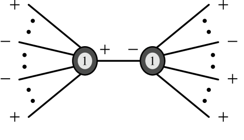
Figure 1: A term in the CSW representation of an NMHV amplitude. The black dot represents the multiparticle pole multiplying the two on-shell amplitudes. The ‘1’ inside the vertex signifies that it is a basic MHV vertex corresponding to a degree 1 curve in twistor space.

The CSW rules then instruct us to write down all tree diagrams with MHV vertices, subject to the constraints that each vertex have exactly two negative-helicity gluons and at least one positive-helicity gluon attached, and that each propagator connect legs of opposite helicity. For amplitudes with two negative-helicity gluons, the vertex with all legs taken on shell is then the amplitude. For each additional negative-helicity gluon, we must add a vertex and a propagator. The number of vertices is thus the number of negative-helicity gluons, less one. For example, to compute amplitudes with three negative-helicity gluons, we must write down all diagrams with two vertices. One of the vertices has two of the external negative-helicity gluons attached to it, while the other has only one. An example of such a diagram is shown in fig. 1.

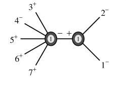
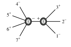
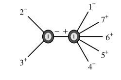
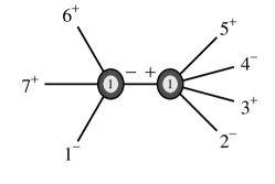
Figure 2: Examples of diagrams for the seven-point NMHV amplitude $A_{7}(1^{-},2^{-},3^{+},4^{-},5^{+},6^{+},7^{+})$.

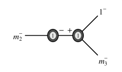
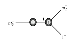
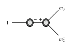
Figure 3: The stripped diagrams for amplitudes with three negative-helicity gluons.

Some diagrams for the amplitude $A_{7}(1^{-},2^{-},3^{+},4^{-},5^{+},6^{+},7^{+})$ are shown in fig. 2. We can classify the diagrams into three sets, according to which of the pairs of negative-helicity gluons ($(1,2)$, $(2,4)$, or $(4,1)$) are attached to the same vertex. Indeed, we can imagine obtaining the set of diagrams by first taking diagrams with only the negative-helicity external gluons indicated, and then adding the positive-helicity gluons in all possible ways consistent with the cyclic ordering. Only three such diagrams are needed to generate the set of diagrams for the seven-point amplitude, or indeed for any $n$-point amplitude $A_{n}(1^{-},2^{+},\ldots,m_{2}^{-},(m_{2}\!+\!1)\vphantom{1}^{+},\ldots,m_{3}^{-},(m_{3}\!+\!1)\vphantom{1}^{+},\ldots,n^{+})$. The corresponding stripped diagrams are shown in fig. 3. Each set of stripped diagrams represents an infinite series of amplitudes, with an arbitrary number of positive-helicity legs.

Using the CSW formulation, we can write down an explicit expression for one such amplitude,

$$\hskip-22.76228ptA_{n}(1^{-},2^{-},3^{+},4^{-},5^{+},\ldots,n^{+})=\vphantom{\sum}$$

$${i\over s_{23}}A_{3}(2^{-},3^{+},(-K_{2,3})\vphantom{1}^{-})A_{n-1}(1^{-},(-K_{1;4\cdots n})\vphantom{1}^{+},4^{-},\ldots,n^{+})$$

$$+\sum_{j_{2}=3}^{4}\sum_{j_{1}=j_{2}+2}^{n+1}{i\over s_{j_{2}\cdots(j_{1}\!-\!1)}}A_{j_{1}-j_{2}+1}(j_{2}^{+},\ldots,4^{-},\ldots,(j_{1}-1)\vphantom{1}^{+},(-K_{j_{2}\cdots(j_{1}\!-\!1)})\vphantom{1}^{-})$$

$$\hphantom{+\sum_{j=m_{2}}^{m_{3}-1}{1\over s_{1\cdots j}}}\hskip 8.53581pt\times A_{n-j_{1}+j_{2}+1}(1^{-},2^{-},\ldots,(j_{2}-1)\vphantom{1}^{+},(-K_{1\cdots(j_{2}\!-\!1);j_{1}\cdots n})\vphantom{1}_{\phantom{1}}^{+}\kern-4.0pt,j_{1}^{+},\ldots,n^{+})$$

$$+\sum_{j=5}^{n}{i\over s_{2\cdots(j-1)}}A_{j-1}(2^{-},3^{+},4^{-},\ldots,(j-1)\vphantom{1}^{+},(-K_{2\cdots(j\!-\!1)})\vphantom{1}^{+})$$ (9)

$$\hphantom{+\sum_{j=m_{2}}^{m_{3}-1}{1\over s_{1\cdots j}}}\hskip 8.53581pt\times A_{n-j+3}(1^{-},(-K_{1;j\cdots n})\vphantom{1}^{-},j^{+},\ldots,n^{+})\,,$$

where all indices are to be understood $\mathop{\rm mod}\nolimits n$. Each term corresponds to a different stripped diagram in fig. 3 with $(m_{2},m_{3})=(2,4)$, and the sums on $j_{1,2}$ correspond to all possible ways of attaching the positive-helicity legs in between each pair of negative-helicity ones.

More generally, in the expression for a general amplitude with three negative-helicity gluons, there are three double sums, each term corresponding to a different stripped diagram,

$$A_{n} (1^{-},2^{+},\ldots,m_{2}^{-},(m_{2}+1)^{+}\kern-4.0pt,\kern 1.0pt\ldots,m_{3}^{-},(m_{3}+1)_{\phantom{1}}^{+}\kern-4.0pt,\kern 1.0pt\ldots,n^{+})=\vphantom{\sum}$$

$$\sum_{j_{1},j_{2}}{i\over s_{j_{2}\cdots(j_{1}\!-\!1)}}A_{j_{1}-j_{2}+1}(\ldots,m_{2}^{-},\ldots)\,A_{n-j_{1}+j_{2}+1}(\ldots,m_{3}^{-},\ldots,1^{-},\ldots)$$

$$+\sum_{j_{1},j_{2}}{i\over s_{j_{2}\cdots(j_{1}\!-\!1)}}A_{j_{1}-j_{2}+1}(\ldots,m_{3}^{-},\ldots)\,A_{n-j_{1}+j_{2}+1}(1^{-},\ldots,m_{2}^{-},\ldots)$$

$$+\sum_{j_{1},j_{2}}{i\over s_{j_{2}\cdots(j_{1}\!-\!1)}}A_{n-j_{1}+j_{2}+1}(1^{-},\ldots)\,A_{j_{1}-j_{2}+1}(\ldots,m_{2}^{-},\ldots,m_{3}^{-},\ldots).$$

Each double sum over $j_{1},j_{2}$ corresponds to the different ways of attaching positive-helicity legs to a given stripped diagram.

III Skeleton Diagrams

Figure 4: The lone MHV skeleton diagram for amplitudes with three negative-helicity gluons.

We can go beyond stripping the diagrams of positive-helicity legs to skinning them of negative-helicity ones too. This will yield what we shall call MHV skeleton diagrams, that is CSW diagrams with all external legs removed. We can obtain the three stripped diagrams of fig. 3 by starting with the lone skeleton diagram shown in fig. 4, and first attaching the negative-helicity external gluons in all inequivalent ways consistent with the cyclic ordering, and the requirement that each vertex have exactly two negative-helicity lines attached to it. There are three independent ways of doing this, each one corresponding to one stripped diagram. We can then attach all positive-helicity external gluons, again in all ways consistent with the cyclic ordering. This gives rise to the double sums in eq. (II). Alternatively, we can attach all external legs in one step. This leads to the following representation for the same amplitude as in eq. (II),

$$A_{n}(1^{+},\ldots,m_{1}^{-},(m_{1}\!+\!1)\vphantom{1}^{+},\ldots,m_{2}^{-},(m_{2}\!+\!1)\vphantom{1}^{+},\ldots,m_{3}^{-},(m_{3}\!+\!1)\vphantom{1}^{+},\ldots,n^{+})=$$

$$\hskip 19.91692pt\sum_{j_{1}=1}^{n}\sum_{j_{2}=j_{1}+1}^{j_{1}-3}{i\over s_{j_{1}\cdots j_{2}}}A_{j_{2}-j_{1}+2\mathop{\rm mod}\nolimits n}(j_{1},\ldots,j_{2},(-K_{j_{1}\cdots j_{2}})\vphantom{1}^{-})$$

$$\hskip 19.91692pt\hphantom{\sum_{j_{1}=1}^{n}\sum_{j_{2}=j_{1}+1}^{j_{1}-3}{i\over s_{j_{1}\cdots j_{2}}}}\hskip 14.22636pt\times A_{j_{1}-j_{2}\mathop{\rm mod}\nolimits n}(j_{2}+1,\ldots,j_{1}-1,(-K_{(j_{2}+1)\cdots(j_{1}-1)})\vphantom{1}^{+}),$$ (11)

where $n>4$; where only terms with one negative helicity between $j_{1}$ and $j_{2}$ (inclusively), and two negative helicities between $j_{2}+1$ and $j_{1}-1$ (inclusively), are included; and where the inner sum and all subscripts should be understood in a cyclic sense, for example

$$\sum_{j=n-4}^{3}\equiv\sum_{j={(n-4)\cdots n,1\cdots 3}}\qquad{\rm\ and\ }\qquad\sum_{j=2}^{-2}\equiv\sum_{j=2}^{n-2}.$$ (12)

Both expressions (II) and (11) are of course equivalent to the sum of all CSW diagrams. Recall that to obtain a twistor-space amplitude, one integrates both over a moduli space of curves in $\mathbb{CP}^{3|4}$, and over the positions of the external particles on the curves. As we shall see in the section VII, the skeleton diagrams encode the type of curves in $\mathbb{CP}^{3|4}$ over which one integrates. The different ways of attaching the external legs to the skeleton correspond in twistor space to the arrangements of the external particle insertions on the curves. The introduction of skeleton diagrams is thus very natural from a twistor-space perspective.

In categorizing the skeleton diagrams, we need to list only the topologically inequivalent ones. In fig. 5 we list the distinct skeleton diagrams for amplitudes with up to five (external) negative helicities. In general with $m$ negative helicities, we must sum over all distinct topologies containing $d=m-1$ MHV vertices linked together in all possible trees. As in eq. (11), we recover the sum over CSW diagrams from the skeleton diagrams by summing over all ways of attaching external legs — positive and negative helicities — respecting the cyclic ordering and the requirement that each MHV vertex have exactly two negative helicity legs attached (including the internal ones). Note that MHV vertices with two negative-helicity legs attached but no positive-helicity ones vanish and should therefore not be included.

Figure 5: The skeleton diagrams with up to six external negative-helicity legs. The numbers inside the circles give the degree of the associated curves in twistor space.

Of course, as the number of negative-helicity legs increases, the number of topologically distinct skeleton diagrams grows exponentially. Moreover, we will have additional sums over ways of attaching legs to vertices.

Is there is a way to tame this growth? In the context of color-ordered Feynman rules, recurrence relations Recurrence ; LightConeRecurrence ; DixonTASI have proven a powerful method of evaluating tree amplitudes, both for analytic and direct numerical purposes. A proper use of recurrence relations recycles information and thereby reduces the computational complexity of evaluating a color-ordered amplitude (for given external helicities) from exponential to polynomial. One might imagine reformulating the CSW rules in a recursive fashion, along the same lines as the recasting of the color-ordered Feynman rules; but with the most obvious approach there are vertices with an arbitrary number of legs. This would lead to terms in the recurrence relations with an arbitrary number of sums, which is what we are seeking to avoid.

There is another way to proceed, generalizing eq. (11), which we find more in the spirit of the twistor-space structure of the amplitudes and the CSW rules. It also sheds light on the non-MHV vertices that arose in the work of Gukov, Motl and Neitzke Gukov . First, we must give a more precise definition of such vertices, which we do in the next section.

IV Non-MHV Vertices

The CSW construction of amplitudes uses MHV vertices, and is dual to integrating over the moduli space of degree one curves in $\mathbb{CP}^{3|4}$. In contrast, Roiban, Spradlin, and Volovich RSV1 ; RSV2 compute amplitudes by integrating over the moduli space of one connected degree $d$ curve. Gukov, Motl, and Neitzke Gukov argued that the two approaches are equivalent by showing that they can both be reduced to an integral over the common boundary of the two moduli spaces. As a by-product of their analysis, they noted the existence of non-MHV vertices, though they did not give explicit expressions for them. A non-MHV vertex corresponds to a twistor-space curve of degree $d=q-1$, where $q>2$ is the number of negative-helicity lines attached to the vertex.

Let us now make precise the notion of non-MHV vertices. In the next section, we will show how to use them to reorganize the CSW construction in a recursive form. Later, we shall also use these vertices to show the equivalence of various twistor-space prescriptions in a field-theory approach, and to determine any associated combinatoric factors.

We can define an $n$-point degree-$d$ non-MHV vertex by copying the set of CSW diagrams used to define an on-shell $n$-point amplitude with $d+1$ negative-helicity external legs, and taking all external legs off shell. That is, a CSW amplitude may be converted to a vertex,

$$A_{n}(1,2,\ldots,n)\longrightarrow V_{n}(1,2,\ldots,n),$$ (13)

by using the same off-shell prescriptions (3) or (6) on all external lines as used for sewing MHV vertices together to form non-MHV amplitudes. It is important that the same light-cone reference momentum used for defining off-shell lines connecting the MHV vertices also be used for the external legs; otherwise this reference momentum will not necessarily drop out of on-shell amplitudes we shall later construct using the non-MHV vertices. Moreover the prescription (6) applies only to the MHV vertices, and not to the propagators connecting them. The latter carry the momenta $K$ and not $k^{\flat}$ used to define the spinors in the vertices. The definition of non-MHV vertices given here is not necessarily unique; in a sense, there are at the very least different ‘gauge’ choices corresponding to different choices of the reference momentum $q$.

Figure 6: The skeleton diagrams for vertices up to degree six. The degrees are indicated by the numbers inside the circles.

We may represent the non-MHV vertices stripped of external lines in terms of skeleton diagrams, as shown in fig. 6. Following the same discussion as for amplitudes, the full vertices are obtained by dressing these skeleton diagrams with off-shell external lines in all possible ways consistent with cyclic ordering, and such that each degree-$d$ vertex has exactly $d+1$ negative helicity lines attached.

Since they are obtained from the CSW diagrams, the non-MHV vertices yield non-MHV amplitudes upon taking the on-shell limit for external momenta. With the original CSW off-shell continuation (3) one should of course divide out the additional spinor factors, that is for an $n$-gluon amplitude,

$$A_{n}(1,\ldots,n)=(-1)^{n}\prod_{p}\left[q\,p\right]^{2}\,\prod_{m}{1\over\left[q\,m\right]^{2}}\times V_{n}(1,\ldots,n)\Bigr{|}_{k_{i}^{2}=0}\,,\hskip 85.35826pti=1,\ldots,n,$$ (14)

where the products run over the positive-helicity legs $p$ and the negative-helicity legs $m$. The off-shell continuation (6) is somewhat simpler since we can recover on-shell amplitudes from the vertices simply by taking the on-shell limit of all external momenta,

$$A_{n}(1,\ldots,n)=V_{n}(1,\ldots,n)\Bigr{|}_{k_{i}^{2}=0}\,,\hskip 85.35826pti=1,\ldots,n.$$ (15)

These equations are reflected in the representation of $A_{n}$ and $V_{n}$ by the same skeleton diagrams.

V Recursive Formulation of Twistor-Inspired Rules

As discussed at the end of section III, the most effective rearrangement of CSW diagrams from a computational point of view is one that recycles as much information as possible as one increases the number of negative-helicity legs. For this we seek a recursive approach.

In formulating such an approach, it is helpful to think of the CSW construction as summing over all inequivalent multi-particle factorizations of a gauge-theory amplitude. In massless gauge theories, amplitudes do not have (full) poles in two-particle invariants. The limit $s_{ij}\rightarrow 0$ corresponds to a collinear limit, and amplitudes go as $1/\sqrt{s_{ij}}$ rather than $1/s_{ij}$ in this limit (the four-point amplitude is an exception, where the limit corresponds to a forward-scattering singularity). These collinear singularities are captured by the MHV vertices. The amplitudes do have singularities in $(n>2)$-particle invariants, which are precisely the propagator poles prescribed by the CSW rules. An expression for an amplitude, written in terms of MHV vertices and propagators, corresponds to the complete factorization in all simultaneously factorizable multi-particle channels. For non-exceptional configurations of external momenta, the same reasoning applies to the non-MHV vertices as defined in the previous section.

However, we could choose to factorize one channel at a time. This would decompose an amplitude into the product of two simpler off-shell amplitudes (or vertices), and one propagator. Indeed, examining any skeleton diagram, we could simply pick one of the internal lines. The contributions corresponding to that skeleton diagram (not yet a complete amplitude) can of course be written as the product of the propagator represented by the given internal line, and the off-shell amplitudes (or vertices) on either side. Similarly, we can represent contributions to non-MHV vertices as products of lower-degree vertices and a propagator joining them.

The seeming problem with such an approach is that there are many possible choices of internal lines, and no clear reason to pick one over another. The most natural solution is to sum over all of them. This overcounts each skeleton diagram by a factor of the number of internal lines; but this overcount is the same for every skeleton diagram contributing to a given amplitude, and hence can be divided out uniformly. Restoring the external legs as before, this gives us a representation of a vertex with $c$ negative helicities in terms of two simpler off-shell vertices and a propagator,

$$V_{n}(1^{+},\ldots,m_{1}^{-},(m_{1}\!+\!1)\vphantom{1}^{+},\ldots,m_{2}^{-},(m_{2}\!+\!1)\vphantom{1}^{+},\ldots,m_{c}^{-},(m_{c}\!+\!1)\vphantom{1}^{+},\ldots,n^{+})=$$

$$\hskip 19.91692pt{1\over(c-2)}\sum_{j_{1}=1}^{n}\sum_{j_{2}=j_{1}+1}^{j_{1}-3}{i\over s_{j_{1}\cdots j_{2}}}V_{j_{2}-j_{1}+2\mathop{\rm mod}\nolimits n}(j_{1},\ldots,j_{2},(-K_{j_{1}\cdots j_{2}})\vphantom{1}^{-})$$ (16)

$$\hskip 11.38109pt\hphantom{{1\over(c-2)}\sum_{j_{1}=1}^{n}\sum_{j_{2}=j_{1}+1}^{j_{1}-3}{i\over s_{j_{1}\cdots j_{2}}}}\hskip 17.07164pt\times V_{j_{1}-j_{2}\mathop{\rm mod}\nolimits n}(j_{2}+1,\ldots,j_{1}-1,(-K_{(j_{2}+1)\cdots(j_{1}-1)})\vphantom{1}^{+})\,,$$

where each term is included only if there is at least one negative-helicity gluon in the cyclic range $[j_{1},j_{2}]$ and at least two in the range $[j_{2}+1,j_{1}-1]$. (Again, as in eq. (11), all indices are to be understood $\mathop{\rm mod}\nolimits n$, and all sums in a cyclic sense eq. (12).) The two vertices are simpler in the sense that each has lower degree, that is fewer negative-helicity legs (including the off-shell ones) than the parent vertex. This means that this equation provides a recurrence relation for evaluating any tree-level non-MHV vertex in massless gauge theory, and via eq. (15), for evaluating any tree-level amplitude. Note that the sum implicitly runs over different degrees for the two vertices on the right-hand side, because the number of negative-helicity external legs in $[j_{1},j_{2}]$ can vary.

Using this recurrence identity, along with the MHV vertices of eq. (8) with additional legs taken off shell, we can compute amplitudes numerically as well as analytically. It is straightforward to implement this equation in computer code; the on-shell conditions expressed in eq. (14) or (15) can be imposed from the beginning of a computation. Indeed, we verified numerically that eq. (16) agrees with a light-cone version of conventional recurrence relations through $n=9$. Although we focus on gluon amplitudes here, with suitable sums over the quantum numbers of internal lines, and fermion or scalar analogs of the vertices of eq. (8), the relation also applies to amplitudes with other massless external states, in non-supersymmetric as well as supersymmetric theories.

We illustrate eq. (16) in fig. 7. To follow the derivation pictorially, start with the complete MHV skeleton diagrams for non-MHV vertices of various degrees, illustrated in fig. 6. Pick each propagator on the right-hand side in turn, and mark it. Group and merge the subdiagrams on either side of the marked propagator into two non-MHV vertices with (say) degrees $d_{1}$ and $d_{2}$ respectively, where $d_{1}+d_{2}=d$, the degree of the corresponding non-MHV vertex on the left-hand side. This gives us one term on the right-hand side of the corresponding equation 16. No matter what its topology, each skeleton diagram contributing to a non-MHV vertex has $d-1$ internal propagators. Hence summing over all possible ways of marking propagators, and then grouping and merging subdiagrams, overcounts by a uniform factor, which we must divide out in eq. (16) and fig. 7. (Note that each individual diagram in fig. 7 actually represents two different ways of attaching the negative-helicity external legs, because there are two different helicity assignments possible for the internal line.) We cannot simply pick one of the groupings, because we will not obtain all required poles in a factorization, or equivalently because some CSW diagrams would end up getting dropped. Other ways of decomposing non-MHV vertices will be discussed in section VI.

Figure 7: A recursive construction of non-MHV vertices.

As an explicit example, consider the degree-four vertex. In fig. 6, we see that it is expressed in terms of two MHV skeleton diagrams. We isolate propagators as above in two different ways, grouping subdiagrams into either degree-three $\times$ degree-one diagrams or into degree-two $\times$ degree-two groups. The first MHV skeleton has two $3\times 1$ groupings while the second has three such groupings. In contrast, there is only a single way to group the first MHV diagram into a $2\times 2$ grouping, and no way to group the second in this manner. Thus each MHV diagram is overcounted three times by the listed collection of non-MHV skeleton diagrams: the first appears twice in $3\times 1$ subdiagrams, and once in $2\times 2$ subdiagrams, while the latter shows up three times in $3\times 1$ subdiagrams.

Similarly, consider the degree-five vertex depicted in fig. 6. This vertex may be expressed in terms of three MHV skeleton diagrams. In the recursive approach we group these into $4\times 1$ + $3\times 2$ skeleton subdiagrams. We can decompose the first MHV skeleton diagram into $4\times 1$ subdiagrams in two ways; the second MHV skeleton diagram can be so decomposed in three ways; and the third MHV skeleton diagram, in four ways. The first skeleton diagram admits two decompositions into $3\times 2$ subdiagrams; the second only one such decomposition, and the last skeleton diagram allows no such decomposition. Summing over the two different decompositions, we find a uniform overcount of a factor of four. More generally, for a degree-$d$ vertex, as explained above, we obtain a uniform overcount of $d-1$ upon summing over all groupings into pairs of non-MHV vertices.

The attentive reader may wonder how the combinatoric factors arise when reversing this process, and expanding the non-MHV vertices back into MHV vertices. They arise in counting the number of ways that the diagram can be re-expanded into MHV skeleton diagrams after reattaching the external negative-helicity gluons in order to recover stripped diagrams. The counting in this direction is thus a bit more involved.

VI Alternative Representations

Besides the computationally useful recursive construction of the previous section, other reorganizations of the MHV skeleton diagrams are possible. Each corresponds to a different combination of curves in twistor space. For example, one can organize the diagrams so that a fixed number of vertices appear in each skeleton diagram; or that only a given number of higher degree vertices appear; or in other ways motivated by topological considerations. The recursive construction presented in the previous section is an example of the first kind of reorganization, with the number of vertices fixed at two.

Figure 8: The degree $d$ vertices can be expressed in terms of one degree two vertex and $d-1$ degree one vertices. There is a uniform overcount of $d-1$ in this case.

Each of these reorganizations may be obtained by merging connected groups of MHV vertices into non-MHV vertices. In each of these cases, we determine all combinatoric or overcount factors directly.

As an example with fixed number of higher-degree vertices, we can arrange to have a single degree-two vertex in each diagram. This rearrangement may not be particularly useful, but does serve to illustrate the principle. This leads to the skeleton diagrams depicted in fig. 8. These diagrams are obtained from the ones in fig. 6 by merging a single pair of directly-connected MHV vertices in each diagram. This gives us one degree-two vertex and $d-2$ degree-one vertices as shown in fig. 8. If we sum over all possible pairings of linked MHV vertices, the skeleton diagrams are again overcounted by a uniform factor of $d-1$ since each diagram has $d-1$ linked pairs. This overcount was already noted in ref. Gukov . Similarly, if we create non-MHV diagrams for a degree-$d$ vertex by grouping and merging MHV vertices so as to collapse $r$ links in all possible ways, the overcount factor is ${d-1\choose r}$.

Figure 9: An alternative set of skeleton diagrams for obtaining non-MHV vertices. In this case, for even degree there is no overcount, while for odd degree there is an overcount by a factor of two. In addition there are relative combinatoric factors between the skeleton diagrams.

A more subtle example arises from trying to balance the degrees of the vertices in a diagram. This reorganization is illustrated in fig. 9. From a twistor-space point of view, it expresses an amplitude as a sum of contributions with differing number of curves. One contribution to the degree $d$ vertex has a propagator connecting a degree-$\lfloor d/2\rfloor$ to a degree-$\lceil d/2\rceil$ vertex, along with a series of ‘bicycle wheel’ diagrams with vertices up to degree $\lfloor(d-1)/2\rfloor$ connected to a central vertex of degree one. ($\lfloor x\rfloor$ is the standard notation for the largest integer less than or equal to $x$, and $\lceil x\rceil$ is that for the smallest integer larger than or equal to $x$.)

This example also illustrates the possibility of relative combinatoric factors. For $d$ even there are no combinatoric or overcount factors while for $d$ odd there is an overall factor of two, as well as relative factors of two between different diagrams.

To derive the combinatoric factors within any given reorganization, we must count the total number of ways each MHV skeleton diagram can be merged to give any of the skeleton diagrams built using non-MHV vertices. We may need to add additional copies of some of the latter diagrams in order to obtain a uniform overcount factor, which we then divide out.

For the degree-five vertex, for example, there are two ways to group and merge the linear skeleton appearing first on the fourth line of fig. 6 into the connected product of a degree-two and a degree-three vertex shown first on the penultimate line of fig. 9. There is one way to group and merge the middle ‘lobster’ diagram into such a product, and one way to group and merge it into the middle diagram on the penultimate line of this figure. There is no grouping to be performed on the last skeleton appearing in fig. 6, so it simply appears as is in fig. 9. However, in order to obtain a uniform overall combinatoric factor, we must take two identical copies of it. To obtain the five vertex, the sum of these non-MHV skeleton diagrams must of course be divided by the overall combinatoric factor of two. As illustrated by the degree-six vertex, this patterns continues in the general form mentioned earlier.

To recover full non-MHV diagrams, we must restore the external legs. Conceptually, we can think of doing this in two steps: first, obtain a set of stripped diagrams by attaching negative-helicity external legs to the skeleton in all possible ways consistent with the cyclic ordering and the degree of the vertices (a degree-$d$ vertex must have $d+1$ negative-helicity gluons including the internal ones). One then attaches the positive-helicity external legs in all possible ways consistent with the cyclic symmetry. Alternatively, we can simply attach the external legs in all ways consistent with cyclic symmetry and the degree of the vertices.

Doing so for the decomposition of the degree-four vertex on the third line of fig. 9, for example, we obtain the following expression,

$$V_{n}^{\hbox{\scriptsize4⃝}}(1^{+},\ldots,m_{1}^{-},(m_{1}\!+\!1)\vphantom{1}^{+},\ldots,m_{2}^{-},(m_{2}\!+\!1)\vphantom{1}^{+},\ldots,m_{5}^{-},(m_{5}\!+\!1)\vphantom{1}^{+},\ldots,n^{+})=$$

$$\hskip 14.22636pt\sum_{j_{1}=1}^{n}\sum_{j_{2}=j_{1}+1\atop N_{-}{[j_{1},j_{2}]}=2}^{j_{1}-3}{i\over s_{j_{1}\cdots j_{2}}}V_{j_{2}-j_{1}+2\mathop{\rm mod}\nolimits n}(j_{1},\ldots,j_{2},(-K_{j_{1}\cdots j_{2}})\vphantom{1}^{-})$$

$$\hskip 14.22636pt\hphantom{\sum_{j_{1}=1}^{n}\sum_{j_{2}=j_{1}+1\atop N_{-}{[j_{1},j_{2}]}=2}^{j_{1}-3}{1\over s_{j_{1}\cdots j_{2}}}}\hskip 17.07164pt\times V_{j_{1}-j_{2}\mathop{\rm mod}\nolimits n}(j_{2}+1,\ldots,j_{1}-1,(-K_{(j_{2}+1)\cdots(j_{1}-1)})\vphantom{1}^{+})$$

$$-\sum_{j_{1}=1}^{n}\sum_{j_{2}=j_{1}+1\atop N_{-}{[j_{1},j_{2}]}=1}^{j_{1}-5}\sum_{j_{3}=j_{2}+1}^{j_{1}-4}\sum_{j_{4}=j_{3}+1\atop 1\leq N_{-}{[j_{3},j_{4}]}\leq 2}^{j_{1}-3}\sum_{j_{5}=j_{4}+1}^{j_{1}-2}\sum_{j_{6}=j_{5}+1\atop 1\leq N_{-}{[j_{5},j_{6}]}\leq 2}^{j_{1}-1}{i\,c(N_{-}{[j_{3},j_{4}]},N_{-}{[j_{5},j_{6}]})\over s_{j_{1}\cdots j_{2}}s_{j_{3}\cdots j_{4}}s_{j_{5}\cdots j_{6}}}$$ (17)

$$\hskip 56.9055pt\times V_{j_{2}-j_{1}+2\mathop{\rm mod}\nolimits n}(j_{1},\ldots,j_{2},(-K_{j_{1}\cdots j_{2}})\vphantom{1}^{-})\,V_{j_{4}-j_{3}+2\mathop{\rm mod}\nolimits n}(j_{3},\ldots,j_{4},(-K_{j_{3}\cdots j_{4}})\vphantom{1}^{\pm})$$

$$\hskip 56.9055pt\times V_{j_{6}-j_{5}+2\mathop{\rm mod}\nolimits n}(j_{5},\ldots,j_{6},(-K_{j_{5}\cdots j_{6}})\vphantom{1}^{\pm})$$

$$\hskip 56.9055pt\times V_{j_{1}+j_{3}+j_{5}-j_{2}-j_{4}-j_{6}\mathop{\rm mod}\nolimits n}(K_{j_{1}\cdots j_{2}}\vphantom{1}^{+},(j_{2}+1),\ldots,(j_{3}-1),K_{j_{3}\cdots j_{4}}\vphantom{1}^{\mp},(j_{4}+1),\ldots,$$

$$\hskip 56.9055pt\hphantom{\times V_{j_{1}+j_{3}+j_{5}-j_{2}-j_{4}-j_{6}\mathop{\rm mod}\nolimits n}()}(j_{5}-1),K_{j_{5}\cdots j_{6}}\vphantom{1}^{\mp},(j_{6}+1),\ldots,(j_{1}-1))$$

where as in eq. (11), all indices should be understood $\mathop{\rm mod}\nolimits n$, and sums in a cyclic sense eq. (12) (note, however, that in the last vertex, $j_{2}+1,\ldots,j_{3}-1$ indicates the legs in between $j_{2}$ and $j_{3}$, that is no legs if $j_{3}-j_{2}=1\mathop{\rm mod}\nolimits n$). Also, the notation $N_{-}{[a,b]}$ denotes the number of negative-helicity gluons in the cyclic range $[a,b]$ (the notation $N_{-}{[a,b]}=d$ in the summation indicates that one should sum only over indices satisfying the constraint), and $c$ is a combinatoric factor,

$$c(n_{1},n_{2})={1\over 5-n_{1}-n_{2}}.$$ (18)

This combinatoric factor arises from our choice of combining the topologically distinct stripped diagrams into a single set of sums, and has nothing to do with combinatoric factors arising from the reorganization of MHV skeleton diagrams into non-MHV ones. It would arise in the CSW construction as well if we made a similar choice of combining the sums. Indeed, the sixfold sum in the second term is exactly the same as would emerge in a direct CSW computation. Like the recurrence relation (16), eq. (17) could be used directly for numerical computations, although we would expect eq. (16) to be more efficient for practical applications.

It is clear that many possible rearrangements of MHV vertices into higher degree ones are possible. These alternative representations are useful for shedding light on the variety of instantonic contributions of the topological string that properly reproduce the amplitudes. Any reorganization of into non-MHV vertices is allowed, so long as one arranges for overcount of CSW diagrams to be uniform. The skeleton diagrams provide a simple means for determining the overcounts and any relative combinatoric factors that may be needed.

VII Relation to Degenerating Curves in Twistor Space

As we have seen in the previous sections, it is easy to construct intermediate prescriptions by merging selected groups of MHV vertices into non-MHV vertices. In this section we relate this field-theoretic construction of intermediate prescriptions to the twistor space construction of Gukov et. al. Gukov .

In section III we obtained skeleton diagrams by skinning the MHV diagrams of all their external legs. As mentioned there, this corresponds in twistor space to focusing on the types of instantons one integrates over, and ignoring the external particle insertions.

The duality between skeleton diagrams and curves in twistor space is straightforward. A skeleton diagram containing only degree-one vertices reproduces a collection of CSW diagrams after reattaching the external legs, and is dual to integrating over the moduli space of intersecting degree-one curves in $\mathbb{CP}^{3|4}$. A vertex of degree $d$ in a skeleton diagram corresponds to a twistor space curve of degree $d$. When two vertices are connected by a line, the corresponding twistor space curves intersect. Vertices which are not directly connected correspond to non-intersecting curves.

The ways in which an MHV skeleton diagram can give rise to one of the non-MHV skeleton diagrams in the desired reorganization are in one-to-one correspondence to the ways a collection of intersecting lines can arise (via degeneration) in the integral over higher-degree curves in twistor space. Skeleton diagrams make counting and indexing the way a curve degenerates straightforward. This allows writing a variety of intermediate prescriptions, as exemplified in section VI, keeping track of combinatoric factors.

Figure 10: The MHV skeleton diagrams for amplitudes with six negative-helicity gluons, and the corresponding degenerations of a twistor space curve of degree five.

As an example, let us focus on the degree-five vertex, which gives rise to amplitudes with six negative-helicity legs. As we have seen, there are quite a few ways to obtain this vertex starting from lower-degree vertices. One can use five MHV vertices as in Section III, or sum over combinations of two vertices of degrees $d_{1}+d_{2}=5$ as in Section V, or over other combinations of vertices as explained in Section VI.

In twistor space, one can similarly obtain this amplitude by integrating over the moduli space of connected degree-five instantons; over the moduli space of all possible pairs of instantons of degrees $d_{1}+d_{2}=5$ linked by a twistor space propagator; or over the moduli space of five degree-one instantons linked by four propagators, etc. As argued in ref. Gukov , the fact that all these integrals give the same result comes from the fact that they all reduce to integrals over a common locus. Roughly speaking, the integral over the moduli space of connected degree-five instantons reduces to one over the part of the moduli space where these curves degenerate into five intersecting lines, while the integral over five lines connected by propagators picks up a contribution from where the propagators shrink to zero size. The integrals appearing in other prescriptions also reduce to integrals over the locus of intersecting degree one curves.

Thus, the intermediate prescriptions we formulate using skeleton diagrams translate directly to twistor space prescriptions in which one integrates over any combination of curves with the right degree, such that the configurations of intersecting lines these curves degenerate into are counted with the same weight. For example, In fig. 10 we show the degenerations of degree-five curves into degree-one curves, along with the corresponding skeleton diagrams — which in this case are nothing but CSW diagrams. The intermediate prescription in fig. 11 consists of summing over two-instanton configurations, with equal weight, and is dual to the recursive formulation discussed in section V. One can also use more unusual representations of non-MHV vertices in section VI to engineer intermediate prescriptions in which different numbers of instantons appear, as in fig. 13.

Figure 11: Skeleton diagrams for the recursive formulation of amplitudes with six negative-helicity legs, and the corresponding degenerations of the degree-five instanton.

In the recursive formulation, in order to obtain amplitudes with $d+1$ negative-helicity legs, one needs to sum over all combinations of two instantons with degrees $d_{1}$ and $d-d_{1}$. Since this sum gives a large overcount, one might naively expect that a single term in this sum gives the correct result. However, for $d\geq 4$ this is never the case. This can either be shown by using skeleton diagrams, or by examining twistor-space instantons.

To see this explicitly, consider the amplitude with six negative-helicity legs discussed above, and imagine trying to obtain it from integrating only over two-instanton configurations of degrees three and two, ignoring two-instanton configurations of degrees one and four. As one can see from fig. 11, the integral over two instantons of degree three and two misses contributions coming from the last term of the right-hand side. This happens because two intersecting curves of degrees two and three can never degenerate into a configuration of lines where one line intersects all the other four. This configuration can only be obtained by degenerating two intersecting curves of degrees one and four.

As discussed in Section V, although this configuration does not appear in the 2–3 degeneration, it does appears in the 1–4 degeneration with a bigger overcount than the diagrams coming from the 2–3 degeneration, so that after summing over all degenerations as in fig. 11 one obtains the full result with a uniform overcounting factor.

Figure 12: The degenerations of a twistor space curve of degree four corresponding to the intermediate prescription in eq. (17).

Figure 13: An alternative prescription for amplitudes with six negative-helicity legs.

Hence, the skeleton diagrams introduced earlier capture all information about the ways in which moduli space curves degenerate, making it easy to count these degenerations, and to produce novel intermediate prescriptions. The twistor-space degenerations corresponding to the alternative decomposition of eq. (17), for example, are displayed in fig. 12. One can also use these diagrams (as in the example displayed in fig. 13) to indirectly predict the ways in which complicated twistor-space curves must degenerate.

VIII Conclusions

In this paper, we have presented explicit formulæ for non-MHV vertices in the twistor-motivated formulation of gauge theory amplitudes. We have constructed them using skeleton diagrams, which are CSW diagrams with external legs removed. We have also made use of these vertices to directly formulate gauge theory ‘intermediate’ prescriptions Gukov for computing tree-level amplitudes. Most notable amongst these intermediate prescriptions are those with only two vertices in any diagram, which give a recursive expression for degree-$d$ vertices in terms of lower-degree ones. Recursive methods have proven to be powerful tools in more conventional diagrammatic approaches to gauge theories, and the recursive formulation given here may well be the most computationally efficient way to reorganize CSW diagrams. The straightforward relation between non-MHV vertices and amplitudes means that the recursive approach offers a powerful method of computing amplitudes. In particular, it allows the computation of amplitudes with an arbitrary number of negative-helicity gluons without the need to keep track of increasingly complicated graph topologies that would arise in MHV diagrams. It would be interesting to solve the recurrence relation explicitly.

Skeleton diagrams correspond to collections of twistor-space curves. Different skeleton diagrams, built out of different vertices, for the same non-MHV amplitude correspond to different intermediate prescriptions for the curves over which one integrates in order to compute that amplitude in twistor space. The descriptions of amplitudes via skeleton diagrams and via twistor-space curves can be thought of as dual. Indeed, our approach, proceeding from CSW diagrams, can be thought of as complementary to the approach of Gukov et al. Gukov . From CSW diagrams, we proceed by defining explicit forms of the non-MHV vertices, on to an understanding of how the integrals over moduli spaces of curves should reduce to the consideration of degenerate curves. This approach allows us to determine combinatoric factors explicitly. It also makes the construction of intermediate prescriptions less mysterious — ultimately, all the intermediate prescriptions are just clever ways of grouping CSW diagrams and merging subdiagrams into vertices. The analysis here illustrates a practical duality between field-theory and topological string-theory approaches. Certain aspects of amplitudes, such as the existence of a CSW construction, are much clearer in twistor space, whereas details of the construction of non-MHV vertices are clearer in field theory.

Although tree-level amplitudes correspond only to the classical theory, deeper understanding of these amplitudes has in the past powered new calculations of loop amplitudes. These explicit calculations have revealed unexpected simplicity and intriguing relations that could not have been guess on general field-theoretic grounds. We can look forward to new results and structures in the quantum theory based on calculations emerging from the CSW construction and related work.

References

- (1) E. Witten, hep-th/0312171.
- (2) V. P. Nair, Phys. Lett. B214:215 (1988).
- (3) S. J. Parke and T. R. Taylor, Phys. Rev. Lett. 56:2459 (1986).
- (4) F. Cachazo, P. Svrcek and E. Witten, hep-th/0403047.
- (5) G. Georgiou and V. V. Khoze, hep-th/0404072.
-
(6)
R. Roiban, M. Spradlin and A. Volovich,
JHEP 0404:012 (2004) [hep-th/0402016];
R. Roiban and A. Volovich, hep-th/0402121. - (7) R. Roiban, M. Spradlin and A. Volovich, hep-th/0403190.
- (8) S. Gukov, L. Motl and A. Neitzke, hep-th/0404085.
- (9) F. A. Berends and W. T. Giele, Nucl. Phys. B306:759 (1988).
- (10) F. A. Berends, H. Kuijf, B. Tausk and W. T. Giele, Nucl. Phys. B357:32 (1991).
- (11) D. A. Kosower, Nucl. Phys. B335:23 (1990).
- (12) N. Berkovits, hep-th/0402045.
- (13) A. Neitzke and C. Vafa, hep-th/0402128.
- (14) W. Siegel, hep-th/0404255.
-
(15)
C. J. Zhu,
JHEP 0404:032 (2004)
[hep-th/0403115];
J. B. Wu and C. J. Zhu, hep-th/0406085. - (16) N. Berkovits and L. Motl, JHEP 0404:056 (2004) [hep-th/0403187].
-
(17)
M. Aganagic and C. Vafa,
hep-th/0403192;
E. Witten, hep-th/0403199. - (18) N. Berkovits and E. Witten, hep-th/0406051.
- (19) Z. Bern, L. J. Dixon, D. C. Dunbar and D. A. Kosower, Nucl. Phys. B425:217 (1994) [hep-ph/9403226].
- (20) Z. Bern, L. J. Dixon, and D. A. Kosower, Nucl. Phys. B437:259 (1995) [hep-ph/9409393].
-
(21)
Z. Bern, L. J. Dixon, D. C. Dunbar and D. A. Kosower,
Nucl. Phys. B435:59 (1995) [hep-ph/9409265];
Z. Bern, L. J. Dixon and D. A. Kosower, Nucl. Phys. Proc. Suppl. 51C:243 (1996) [hep-ph/9606378];
Z. Bern, L. J. Dixon and D. A. Kosower, Ann. Rev. Nucl. Part. Sci. 46:109 (1996) [hep-ph/9602280];
Z. Bern and A. G. Morgan, Nucl. Phys. B467:479 (1996) [hep-ph/9511336];
Z. Bern, L. J. Dixon and D. A. Kosower, hep-ph/0404293. - (22) Z. Bern, L. J. Dixon, D. C. Dunbar and D. A. Kosower, Nucl. Phys. B435:59 (1995) [hep-ph/9409265].
-
(23)
J. A. Minahan and K. Zarembo,
JHEP 0303:013 (2003)
[hep-th/0212208];
N. Beisert, C. Kristjansen and M. Staudacher, Nucl. Phys. B664:131 (2003) [hep-th/0303060];
I. Bena, J. Polchinski and R. Roiban, Phys. Rev. D69:046002 (2004) [hep-th/0305116];
N. Beisert, Nucl. Phys. B676:3 (2004) [hep-th/0307015];
N. Beisert and M. Staudacher, Nucl. Phys. B670:439 (2003) [hep-th/0307042];
L. Dolan, C. R. Nappi and E. Witten, JHEP 0310:017 (2003) [hep-th/0308089];
G. Arutyunov and M. Staudacher, JHEP 0403:004 (2004) [hep-th/0310182];
L. Dolan, C. R. Nappi and E. Witten, in Proceedings of the 3rd International Symposium on Quantum Theory and Symmetries (QTS3), Cincinnati, Ohio, Sept. 10–14, 2003 [hep-th/0401243]. -
(24)
C. Anastasiou, Z. Bern, L. J. Dixon and D. A. Kosower,
Phys. Rev. Lett. 91:251602 (2003)
[hep-th/0309040];
C. Anastasiou, L. J. Dixon, Z. Bern and D. A. Kosower, in Proceedings of the 3rd International Symposium on Quantum Theory and Symmetries (QTS3), Cincinnati, Ohio, Sept. 10–14, 2003 [hep-th/0402053]. -
(25)
F. A. Berends and W. Giele,
Nucl. Phys. B294:700 (1987);
D. A. Kosower, B.-H. Lee and V. P. Nair, Phys. Lett. 201B:85 (1988);
M. Mangano, S. Parke and Z. Xu, Nucl. Phys. B298:653 (1988);
Z. Bern and D. A. Kosower, Nucl. Phys. B362:389 (1991). -
(26)
F. A. Berends, R. Kleiss, P. De Causmaecker, R. Gastmans, and T. T. Wu,
Phys. Lett. 103B:124 (1981);
P. De Causmaeker, R. Gastmans, W. Troost, and T. T. Wu, Nucl. Phys. B206:53 (1982);
Z. Xu, D.-H. Zhang, L. Chang, Tsinghua University preprint TUTP–84/3 (1984), unpublished;
R. Kleiss and W. J. Stirling, Nucl. Phys. B262:235 (1985);
J. F. Gunion and Z. Kunszt, Phys. Lett. 161B:333 (1985);
Z. Xu, D.-H. Zhang, and L. Chang, Nucl. Phys. B291:392 (1987). - (27) D. A. Kosower, hep-th/0406175.
-
(28)
M. T. Grisaru, H. N. Pendleton and P. van Nieuwenhuizen,
Phys. Rev. D15:996 (1977);
M. T. Grisaru and H. N. Pendleton, Nucl. Phys. B124:81 (1977);
S. J. Parke and T. R. Taylor, Phys. Lett. B157:81 (1985) [Erratum-ibid. B174:465 (1986)];
Z. Kunszt, Nucl. Phys. B271:333 (1986). - (29) L. J. Dixon, in QCD & Beyond: Proceedings of TASI ’95, ed. D. E. Soper (World Scientific, 1996) [hep-ph/9601359].