Low Energy Branes, Effective Theory and Cosmology

Abstract

The low energy regime of cosmological BPS-brane configurations with a bulk scalar field is studied. We construct a systematic method to obtain five-dimensional solutions to the full system of equations governing the geometry and dynamics of the bulk. This is done for an arbitrary bulk scalar field potential and taking into account the presence of matter on the branes. The method, valid in the low energy regime, is a linear expansion of the system about the static vacuum solution. Additionally, we develop a four-dimensional effective theory describing the evolution of the system. At the lowest order in the expansion, the effective theory is a bi-scalar tensor theory of gravity. One of the main features of this theory is that the scalar fields can be stabilized naturally without the introduction of additional mechanisms, allowing satisfactory agreement between the model and current observational constraints. The special case of the Randall-Sundrum model is discussed.

I Introduction

Brane-world models have become an important subject of research in recent years. The simple and intuitive notion that the standard model of physics is embedded in a hypersurface (brane), located in a higher dimensional space (bulk), has significant implications for gravity, high energy physics and cosmology. It is strongly motivated by recent developments in string theory and its extended version, M-theory Harova-Wiiten 1 ; Harova-Wiiten 2 ; Lukas etal . Additionally, it has been proposed on a phenomenological basis Akama ; Rubakov ; Visser to address many questions which cannot be answered within the context of the conventional standard model of physics, such as the hierarchy problem and the cosmological constant problem Antoniadis etal ; Antoniadis ; RS1 ; RS2 ; Arkani etal ; Forste etal .

The basic idea is that gravity -and possibly other forces- propagate freely in the bulk, while the Standard Model’s fields are confined to a 4-dimensional brane (see brax-bruck ; Langlois ; Maartens ; brax-bruck-davis for comprehensive reviews on brane-world models). In this type of model, constraints on the size of extra dimensions are much weaker than in Kaluza-Klein theories Kaluza-Klein , although, Newton’s law of gravity is still sensitive to the presence of extra dimensions. Gravity has been tested only to a tenth of millimeter Hoyle etal , therefore, possible deviations to Newton’s law, below that scale, can be envisaged. In general, one of the main modifications to general relativity offered by brane models, is the appearance, in the effective Einstein’s equations of the system, of novel terms that depend quadratically on the energy-momentum tensor of the matter content of the observed Universe. When these terms can be neglected the brane system is in the low energy regime. It is well known that the most recent cosmological era must be considered within the low energy regime. Despite this fact, there are still important modifications to general relativity that must be considered, and current observational constraints are highly relevant for the phenomenology of brane models.

Cosmologically speaking, the evolution of the branes in the bulk is directly related to the evolution of the observed Universe Flanagan etal 1 ; Bruck etal . So far, most of cosmological considerations of brane-worlds have been centered on the models proposed by Randall and Sundrum RS1 ; RS2 . They considered warped geometries in which the bulk-space is a slice of Anti de Sitter space-time. One of the main problems of these scenarios is the stabilization of new extra degrees of freedom appearing from the construction. More precisely, when the four-dimensional equations of motion for the branes are considered, a new scalar degree of freedom, the radion, emerges. The stabilization of the radion is an important phenomenological problem, and many different mechanisms to stabilize it have been proposed Goldberger-Wise ; Lesgourgues etal . Clearly, brane models which only consider the presence of gravity in the bulk, such as the Randall-Sundrum model, are not fully satisfactory from a theoretical point of view. There is no reason a priori for gravity to be the only force propagating in the bulk, and other unmeasured forces may also be present. For instance, string theory predicts the existence of the dilaton field which acts as a massless partner of the graviton. If such forces are present in the bulk, they should be suppressed by some stabilization mechanism in order to evade observation (similar to the case of the radion field in the Randall-Sundrum model). The problem of finding a stabilization mechanism is an active field of research.

In this paper we are going to consider a fairly general brane-world model (BPS-branes), which has been motivated as a supersymmetric extension of the Randall–Sundrum model Bergshoeff etal ; Binetruy etal ; Davis & Brax ; Csaki etal ; Youm (see Flanagan etal 2 ; DeWolfe etal for phenomenological motivations). It consists of a five-dimensional bulk space with a scalar field $\psi$, bounded by two branes, $\sigma_{1}$ and $\sigma_{2}$. The main property of this system is a special boundary condition that holds between the branes and the bulk fields, which allows the branes to be located anywhere in the background without obstruction. In particular, a special relation exists between the scalar field potential $U(\psi)$, defined in the bulk, and the brane tensions $U_{B}(\psi^{1})$ and $U_{B}(\psi^{2})$ defined at the position of the branes. This is the BPS condition. Due to the complexity of this set up, the main efforts of previous works have been focused on the special case $U_{B}(\psi)\propto e^{\alpha\psi}$, where $\alpha$ is a parameter of the theory Br-CvdB-ACD-Rh ; Kobayashi-Koyama . This particular potential is well motivated by supergravity in singular spaces and string theory. For instance, when $\alpha=0$, the Randall-Sundrum model is retrieved, meanwhile, for larger values, $\alpha=O(1)$, one obtains the low–energy effective action of heterotic $M$–theory, taking into account the volume of the Calabi–Yau manifold Lukas . Nevertheless, other classes of potentials also have physical motivation and should be considered. For instance, in 5-dimensional supergravity, one can expect the linear combination $U_{B}(\psi)=V_{1}e^{\alpha_{1}\psi}+V_{2}e^{\alpha_{2}\psi}$, where $\alpha_{1}$ and $\alpha_{2}$ are given numbers Davis & Brax . It must be stated, however, that up to now the problem of assuming an arbitrary potential $U_{B}(\psi)$ has not been considered in detail, and therefore, the low energy regime of this type of system is not well understood. For example, it is not known how the gravitational fields nor the bulk scalar field behave near the branes, and the general belief is that these issues should be investigated via numerical techniques.

Here we study the low energy regime of brane-models with a bulk scalar field. One of the most important aspects is that we shall not restrict our treatment to any particular choice of the BPS potential, allowing a clearer understanding of 5-dimensional BPS systems, and focus our study on the problems mentioned previously. In particular we shall develop a systematic method to obtain 5-dimensional solutions for the gravitational fields and the bulk scalar fields. Additionally, by adopting the projective approach, we develop an effective 4-dimensional theory, valid in the low energy regime, and indicate that it is equivalent to the moduli-space approximation. This effective theory is a bi-scalar tensor theory of gravity of the form:

$$S = \frac{1}{k\kappa_{5}^{2}}\int d^{4}x\sqrt{-g}\bigg{[}R-\frac{3}{4}g^{\mu\nu}\gamma_{ab}\partial_{\mu}\psi^{a}\partial_{\nu}\psi^{b}-\frac{3}{4}V\bigg{]}$$ (1)

$$+S_{1}[\Psi_{1},A_{1}^{2}g_{\mu\nu}]+S_{2}[\Psi_{2},A_{2}^{2}g_{\mu\nu}],$$

where $a=1,2$ labels the branes, $\psi^{a}$ corresponds to the projected bulk scalar field at the brane $\sigma_{a}$, $\gamma_{ab}$ is a $\sigma$-model metric of the bi-scalar theory, $S_{1}$ and $S_{2}$ are the actions for matter fields $\Psi_{1}$ and $\Psi_{2}$ living in the respective branes, and $A_{1}$ and $A_{2}$ are warp factors dependent on the scalar fields. Obtaining this effective theory is a great achievement that allows the study of this class of models within the approach and usual techniques of multi-scalar tensor theories Damour-Esposito ; Damour .

This paper is organized as follows: In Section II, we review brane systems with a bulk scalar field. There, we illustrate in a more technical way some of the problems that this paper addresses. In Section III, we work out and analyze the static solutions for the vacuum configuration of BPS-branes. This enables us to construct the low energy regime expansion in Section IV. Then, in Section V, we develop the four-dimensional effective theory valid in the low energy regime. There, we will focus our attention on the zeroth order effective theory which is a bi-scalar tensor theory of gravity. In Section VI, we study the cosmology of the effective theory. For instance, we consider the constraints coming from current observations on deviations to General Relativity and analyze the stabilization problem of BPS-systems. It will be found that, in order to stabilize this type of system it is enough to have the appropriate potential $U_{B}$, and therefore no exotic mechanisms are required in general. The conclusions are summarized in Section VII.

II BPS-Branes with a Bulk Scalar Field

We start this section with the introduction of 5-dimensional BPS configurations, deriving the 5-dimensional equations of motion governing the dynamics of the system and deducing the projected equations at the position of the branes. These equations depend on the configuration of the bulk as well as on the matter content in the branes; we analyze the difficulties arising from this dependence to find solutions to realistic cosmological configurations.

II.1 Basic Configuration

Let us consider a 5-dimensional manifold $M$ provided with a coordinate system $X^{A}$, with $A=0,\ldots,4$. We shall assume the special topology $M=\sigma\times S^{1}/Z_{2}$, where $\sigma$ is a fixed 4-dimensional lorentzian manifold without boundaries and $S^{1}/Z_{2}$ is the orbifold constructed from the 1-dimensional circle with points identified through a $Z_{2}$-symmetry. The manifold $M$ is bounded by two branes located at the fixed points of $S^{1}/Z_{2}$. Let us denote the brane-surfaces by $\sigma_{1}$ and $\sigma_{2}$ respectively. We shall usually refer to the space bounded by the branes as the bulk space. We will consider the existence of a bulk scalar field $\psi$ living in $M$ with boundary values, $\psi^{1}$ and $\psi^{2}$, at the branes. Consider also the presence of a bulk potential $\mathcal{U}(\psi)$ and brane tensions $\mathcal{V}_{1}(\psi^{1})$ and $\mathcal{V}_{2}(\psi^{2})$ (which are potentials for the boundary values $\psi^{1}$ and $\psi^{2}$). Additionally, we will consider the existence of matter fields $\Psi_{1}$ and $\Psi_{2}$ confined to the branes. Figure 1 shows a schematic representation of the present configuration.

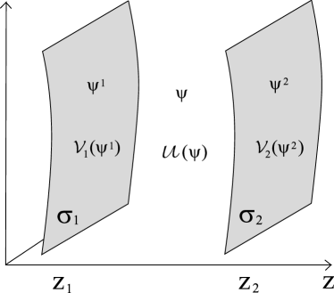
Figure 1: Schematic representation of the 5-dimensional brane configuration. In the bulk there is a scalar field $\psi$ with a bulk potential $\mathcal{U}(\psi)$. Additionally, the bulk-space is bounded by branes, $\sigma_{1}$ and $\sigma_{2}$, with tensions given by $\mathcal{V}_{1}(\psi^{1})$ and $\mathcal{V}_{2}(\psi^{2})$ respectively, where $\psi^{1}$ and $\psi^{2}$ are the boundary values of $\psi$.

Given the present topology, it is appropriate to introduce foliations with a coordinate system $x^{\mu}$ describing $\sigma$ (as well as the branes $\sigma_{1}$ and $\sigma_{2}$) where $\mu=0,\ldots,3$. Additionally, we can introduce a coordinate $z$ describing the $S^{1}/Z_{2}$ orbifold and parameterizing the foliations. With this decomposition the following form of the line element can be used to describe $M$:

$$ds^{2}=(N^{2}+N^{\rho}N_{\rho})dz^{2}+2N_{\mu}dx^{\mu}dz+g_{\mu\nu}dx^{\mu}dx^{\nu}\!.$$ (2)

Here $N$ and $N^{\mu}$ are the lapse and shift functions for the extra dimensional coordinate $z$ and, therefore, they can be defined up to a gauge choice (for example, the gaussian normal coordinate system is such that $N^{\mu}=0$). Additionally, $g_{\mu\nu}$ is the pullback of the induced metric on the 4–dimensional foliations, with the $(-,+,+,+)$ signature. The branes are located at the fixed points of the $S^{1}/Z_{2}$ orbifold, denoted by $z=z_{1}$ and $z=z_{2}$, where $1$ and $2$ are the labels for the first and second branes, $\sigma_{1}$ and $\sigma_{2}$. Without loss of generality, we shall take $z_{1}<z_{2}$.

The total action of the system is

$$S_{\mathrm{tot}}=S_{\mathrm{G}}+S_{\mathrm{bulk}}+S_{\mathrm{BR}},$$ (3)

where $S_{\mathrm{G}}$ is the action describing the pure gravitational part and is given by $S_{\mathrm{G}}=S_{\mathrm{EH}}+S_{\mathrm{GH}}$, with $S_{\mathrm{EH}}$ the Einstein–Hilbert action and $S_{\mathrm{GH}}$ the Gibbons–Hawking boundary terms; $S_{\mathrm{bulk}}$ is the action for the matter fields living in the bulk, which can be decomposed into $S_{\mathrm{bulk}}=S_{\psi}+S_{\mathrm{m}}$. Here $S_{\psi}$ is the action for the bulk scalar field $\psi$ (including its boundary terms), while $S_{\mathrm{m}}$ is the action for other matter fields (in the present work we will not specify this part of the theory). Finally $S_{\mathrm{BR}}$ is the action for the matter fields, $\Psi_{1}$ and $\Psi_{2}$, confined to the branes.

Let us see in more detail the different contributions appearing in equation (3). First, note that with the present parameterization for $M$, we can write an infinitesimal proper element of volume as $dV=dzd^{4}x\sqrt{-g}N$. Then, it is possible to express $S_{\mathrm{G}}$ in the following way

$$S_{\mathrm{G}} = S_{\mathrm{EH}}+S_{\mathrm{GH}}$$

$$= \frac{1}{2\kappa_{5}^{2}}\int_{S^{1}\!/Z_{2}}\!\!\!\!\!\!\!dz\int_{\sigma}\!\!d^{\,4}x\sqrt{-g}\,N\big{(}R-[K_{\mu\nu}K^{\mu\nu}-K^{2}]\big{)},$$

where $R$ is the four-dimensional Ricci scalar constructed from $g_{\mu\nu}$, and $\kappa_{5}^{2}=8\pi G_{5}$, with $G_{5}$ the five-dimensional Newton’s constant. Additionally, $K_{\mu\nu}=\left[g_{\mu\nu}^{\prime}-\nabla_{\mu}N_{\nu}-\nabla_{\nu}N_{\mu}\right]/2N$ is the extrinsic curvature of the foliations and $K$ its trace (the prime denotes derivatives in terms of $z$, that is ${}^{\prime}=\partial_{z}$, and covariant derivatives, $\nabla_{\mu}$, are constructed from the induced metric $g_{\mu\nu}$ in the standard way). On the other hand the action for the bulk scalar field, $S_{\psi}$, can be written in the form

$$S_{\psi} = -\frac{3}{8\kappa_{5}^{2}}\int dz\,d^{4}x\sqrt{-g}\,N\bigg{[}\bigg{(}\frac{\psi^{\prime}}{N}\bigg{)}^{2}+(\partial\psi)^{2}$$ (5)

$$-2\frac{N^{\mu}}{N^{2}}\,\partial_{\mu}\psi\,\partial_{z}\psi+\mathcal{U}(\psi)\bigg{]}+S_{\psi}^{\,1}+S_{\psi}^{\,2}\!,$$

where $S_{\psi}^{\,1}$ and $S_{\psi}^{\,2}$ are boundary terms given by

$$S_{\psi}^{\,1} = -\frac{3}{2\kappa_{5}^{2}}\int_{\sigma_{1}}\!\!\!d^{4}x\sqrt{-g}\,\mathcal{V}_{1}(\psi^{1}),$$ (6)

$$S_{\psi}^{\,2} = +\frac{3}{2\kappa_{5}^{2}}\int_{\sigma_{2}}\!\!\!d^{4}x\sqrt{-g}\,\mathcal{V}_{2}(\psi^{2}),$$ (7)

at the respective positions, $z_{1}$ and $z_{2}$. In the above expressions $\mathcal{U}(\psi)$ is the bulk scalar field potential, while $\mathcal{V}_{1}(\psi^{1})$ and $\mathcal{V}_{2}(\psi^{2})$ are boundary potentials defined at the positions of the branes (also referred as the brane tensions). In the present case (BPS-configurations), we shall consider the following general form for the potentials:

$$\mathcal{U} = U+u,$$ (8)

$$\mathcal{V}_{1} = U_{B}+v_{1},$$ (9)

$$\mathcal{V}_{2} = U_{B}+v_{2},$$ (10)

where $U$ and $U_{B}$ are the bulk and brane superpotentials, and the potentials $u$, $v_{1}$ and $v_{2}$ are such that $|u|\ll|U|$ and $|v_{1}|,|v_{2}|\ll|U_{B}|$. In this way, the system is dominated by the superpotentials $U$ and $U_{B}$. The most important characteristic of this class of system is the relation between $U$ and $U_{B}$ (the BPS-relation), given by:

$$U=\left(\partial_{\psi}U_{B}\right)^{2}-U_{B}^{2}.$$ (11)

As we shall see later in more detail, the BPS property mentioned earlier (the fact that the branes can be located anywhere in the background, without obstruction) comes from the relation above. This specific configuration, when the potentials $u,v_{1},v_{2}=0$ and no fields other than the bulk scalar field are present, is referred as the BPS configuration. It emerges, for instance, in models like $N=2$ supergravity with vector multiplets in the bulk Davis & Brax . More generally, it can be regarded as a supersymmetric extension of the Randall-Sundrum model. In particular when $U_{B}$ is the constant potential, the Randall–Sundrum model is recovered with a bulk cosmological constant $\Lambda_{5}=(3/8)U=-(3/8)\,U_{B}^{2}$, and the usual fine tuning condition is given by equation (11). The presence of the potentials $u$, $v_{1}$ and $v_{2}$ are generally expected from supersymmetry breaking effects. However, their specific form is not known and, up to now, they must be arbitrarily postulated brax-chatillon .

Finally, for the matter fields confined to the branes, we shall consider the standard action:

$$S_{\mathrm{BR}}=S_{1}[\Psi_{1},g_{\mu\nu}(z_{1})]+S_{2}[\Psi_{2},g_{\mu\nu}(z_{2})],$$ (12)

where $\Psi_{1}$ and $\Psi_{2}$ denote the respective matter fields, and $g_{\mu\nu}(z_{a})$ is the induced metric at position $z_{a}$. In this article we shall assume that the matter fields are minimally coupled to the bulk scalar field. That is to say, we will assume that $S_{\mathrm{BR}}$ does not depend explicitly on $\psi$. Nevertheless, it is important to point out that, in general, one should expect some nontrivial coupling between the bulk scalar field $\psi$ and the matter fields $\Psi_{1}$ and $\Psi_{2}$, that could lead to the variation of constants in the brane-world scenario Palma etal . Despite these comments, we show that, in a minimally coupled system, an effective coupling is generated between the matter fields and the bulk scalar field.

II.2 Equations of Motion

In this subsection we derive the equations of motion governing the dynamics of the fields living in the bulk. These equations are obtained by varying the action $S_{\mathrm{tot}}$ with respect to the gravitational and bulk scalar fields, without taking into account the boundary terms. These will be considered in the next subsection, in order to deduce a set of boundary conditions for the bulk fields.

The 5-dimensional Einstein’s equations of the system can be derived through the variation of the total action $S_{\mathrm{tot}}$ with respect to $N$, $N_{\mu}$ and $g_{\mu\nu}$. Respectively, these equations are found to be:

$$R+\left[K_{\mu\nu}K^{\mu\nu}-K^{2}\right]=2\kappa_{5}^{2}\,\tilde{S},$$ (13)

$$\nabla_{\mu}\left[K^{\mu}_{\nu}-K\delta^{\mu}_{\nu}\right]=-\kappa_{5}^{2}\,\tilde{J}_{\nu},$$ (14)

$$G_{\mu\nu}+E_{\mu\nu}=\frac{1}{2}g_{\mu\nu}\left[K_{\rho\sigma}K^{\rho\sigma}-K^{2}\right]+KK_{\mu\nu}$$

$$-K^{\sigma}_{\mu}K_{\sigma\nu}+\frac{2}{3}\kappa_{5}^{2}\bigg{[}\tilde{T}_{\mu\nu}-\frac{1}{4}g_{\mu\nu}(\tilde{T}_{\sigma}^{\sigma}+3\tilde{S})\bigg{]}.$$ (15)

The above set of equations deserves a detailed description. $G_{\mu\nu}$, in (15), is the Einstein tensor constructed from the induced metric $g_{\mu\nu}$. The quantities $\tilde{T}_{\mu\nu}$, $\tilde{J}_{\mu}$, and $\tilde{S}$ are the 4-dimensional stress energy-momentum tensor, vector and scalar respectively, characterising the matter content in the bulk space. They are defined as

$$\tilde{S} = -\frac{1}{\sqrt{-g}}\frac{\delta S_{\mathrm{bulk}}}{\delta N},$$

$$\tilde{J}_{\mu} = -\frac{1}{\sqrt{-g}}\frac{\delta S_{\mathrm{bulk}}}{\delta N^{\mu}},$$

$$\tilde{T}_{\mu\nu} = -\frac{2}{N\sqrt{-g}}\frac{\delta S_{\mathrm{bulk}}}{\delta g^{\mu\nu}},$$ (16)

where $S_{\mathrm{bulk}}=S_{\psi}+S_{\mathrm{m}}$ is the action for the matter fields living in the bulk. The above quantities are decompositions of the usual 5-dimensional stress energy-momentum tensor, $T_{AB}$. To be more specific, the definitions in (16) satisfy: $\tilde{T}_{\mu\nu}=X_{,\,\mu}^{A}\,X_{,\,\nu}^{B}\,T_{AB}$, $\tilde{J}_{\mu}=-X_{,\,\mu}^{A}\,n^{B}\,T_{AB}$, and $\tilde{S}=-n^{A}n^{B}\,T_{AB}$, where $X_{,\,\mu}^{A}$ is the pullback between the coordinate system $x^{\mu}$ of the foliations and the 5-dimensional coordinate system $X^{A}$ of $M$, and where $n^{A}$ is the unit-vector field normal to the foliations. In particular, the contributions coming from the scalar field action, $S_{\psi}$, are given by:

$$\tilde{S}^{(\psi)} = -\frac{3}{8\kappa_{5}^{2}}\bigg{[}\frac{1}{N^{2}}(\psi^{\prime})^{2}-2\frac{N^{\mu}}{N^{2}}\,\partial_{\mu}\psi\,\partial_{z}\psi-(\partial\psi)^{2}-\mathcal{U}\bigg{]},$$

$$\tilde{J}^{(\psi)}_{\mu} = -\frac{3}{4\kappa_{5}^{2}}\frac{1}{N}\,\partial_{z}\psi\partial_{\mu}\psi,$$

$$\tilde{T}^{(\psi)}_{\mu\nu} = -\frac{3}{4\kappa_{5}^{2}}\bigg{[}\frac{1}{2}g_{\mu\nu}\bigg{(}\frac{1}{N^{2}}(\psi^{\prime})^{2}-2\frac{N^{\mu}}{N^{2}}\,\partial_{\mu}\psi\,\partial_{z}\psi$$ (17)

$$+(\partial\psi)^{2}+\mathcal{U}\bigg{)}-\partial_{\mu}\psi\partial_{\nu}\psi\bigg{]}.$$

Also in (15) is $E_{\mu\nu}$, the projection of the 5-dimensional Weyl tensor, $C^{C}_{\,\,\,\,ADB}$, on the foliations given by $E_{\mu\nu}=X_{,\,\mu}^{A}X_{,\,\nu}^{B}\,n_{C}\,n^{D}\,C^{C}_{\,\,\,ADB}$. In the present set up, this can be written as:

$$E_{\mu\nu} = K_{\mu}^{\alpha}K_{\alpha\nu}-\frac{1}{N}\left(\nabla_{\mu}\nabla_{\nu}N+\pounds_{Nn}K_{\mu\nu}\right)$$ (18)

$$-\frac{1}{3}\kappa_{5}^{2}\left[\tilde{T}_{\mu\nu}-\frac{1}{2}g_{\mu\nu}(\tilde{T}_{\sigma}^{\sigma}+\tilde{S})\right],$$

where $\pounds_{Nn}$ is the Lie derivative along the vector field $Nn^{A}$. At this point it is convenient to adopt the gauge choice $N^{\mu}=0$, which corresponds to the choice of gaussian normal coordinates. With this gauge, one has $\pounds_{Nn}=\partial_{z}$, and the treatment of the entire system is greatly simplified. Next, we can obtain the equation of motion for the bulk scalar field $\psi$. Varying the action with respect to $\psi$ gives:

$$g^{\mu\nu}\nabla_{\mu}\left(N\partial_{\nu}\psi\right)+\left(\psi^{\prime}/N\right)^{\prime}+K\psi^{\prime}=\frac{N}{2}\frac{\partial\mathcal{U}}{\partial\psi}.$$ (19)

(Recall that we are now using $N^{\mu}=0$).

It is possible to see that equations (13) and (15) are the dynamical equations for the gravitational sector (notice that second order derivatives in terms of $z$ are only present in the projected Weyl tensor $E_{\mu\nu}$). Meanwhile, equation (14) constitutes a restriction for the extrinsic curvature $K_{\mu\nu}$ in terms of the matter content of the bulk. As we shall soon see in more detail, the conservation of energy-momentum on the branes is a direct consequence of equation (14).

II.3 Boundary Conditions

We can now turn to the boundaries of the system. The former variations leading to equations (13)-(15) and (19) also give rise to boundary conditions that must be respected by the bulk fields at positions $z_{1}$ and $z_{2}$. They emerge when we take into account the boundary terms present in the action (including the matter fields in the branes). For the first brane, $\sigma_{1}$, these conditions are found to be:

$$\{K_{\mu\nu}-g_{\mu\nu}K\}|_{z_{1}} = \frac{3}{2}\left[U_{B}+v_{1}\right]\,g_{\mu\nu}-\kappa_{5}^{2}T_{\mu\nu}^{1},\quad$$ (20)

$$\frac{1}{2}\{\psi^{\prime}/N\}|_{z_{1}} = \partial_{\psi}\left[U_{B}+v_{1}\right],$$ (21)

while for the second brane, $\sigma_{2}$, these conditions are:

$$\{K_{\mu\nu}-g_{\mu\nu}K\}|_{z_{2}} = -\frac{3}{2}\left[U_{B}+v_{2}\right]\,g_{\mu\nu}-\kappa_{5}^{2}T_{\mu\nu}^{2},\quad$$ (22)

$$\frac{1}{2}\{\psi^{\prime}/N\}|_{z_{2}} = -\partial_{\psi}\left[U_{B}+v_{2}\right].$$ (23)

Equations (20) and (22) are the Israel matching conditions and equations (21) and (23) are the BPS matching conditions for the bulk scalar field. In the previous expressions the brackets denote the difference between the evaluation of quantities at both sides of the branes, i.e $\{f\}|_{z}=\lim_{\epsilon\rightarrow 0}[f(z+\epsilon)-f(z-\epsilon)]$. Additionally, $T^{a}_{\mu\nu}$ denotes the energy–momentum tensors of the matter content in the brane $\sigma_{a}$, and is defined by the standard expression:

$$T^{a}_{\mu\nu}=-\frac{2}{\sqrt{-g}}\frac{\delta S_{a}}{\delta g^{\mu\nu}}\bigg{|}_{z_{a}}.$$ (24)

Since we are considering an orbifold with a $Z_{2}$-symmetry, and the branes are positioned at the fixed points, the conditions (20)-(23) can be rewritten as

$$K_{\mu\nu}-g_{\mu\nu}K = \frac{3}{4}\left[U_{B}+v_{1}\right]\,g_{\mu\nu}-\frac{\kappa_{5}^{2}}{2}T_{\mu\nu}^{1},$$ (25)

$$\psi^{\prime} = N\,\partial_{\psi}\left[U_{B}+v_{1}\right],$$ (26)

for the first brane, $\sigma_{1}$, and

$$K_{\mu\nu}-g_{\mu\nu}K = \frac{3}{4}\left[U_{B}+v_{2}\right]\,g_{\mu\nu}+\frac{\kappa_{5}^{2}}{2}T_{\mu\nu}^{2},$$ (27)

$$\psi^{\prime} = N\,\partial_{\psi}\left[U_{B}+v_{2}\right],$$ (28)

for the second brane, $\sigma_{2}$. These conditions are of utmost importance. They relate the geometry of the bulk with the matter content in the branes. In the next subsection we shall examine in more detail how these conditions are related to the 4-dimensional effective equations in the branes and analyze some of the open questions.

II.4 Short Analysis and Open Questions

Equations (13)-(15) and (19) can be evaluated at the position of the branes, with the help of the boundary conditions (25)-(28), to obtain a set of 4-dimensional effective equations. This is the projective approach. For instance, evaluating equations (13) and (15) at the position of the first brane, we find:

$$R=-\frac{\kappa_{5}^{2}}{4}\mathcal{V}_{1}T-g^{\mu\nu}\Pi_{\mu\nu}+\frac{3}{4}W$$ (29)

$${}+\frac{3}{4}(\partial\psi)^{2}-g^{\mu\nu}\Theta^{(\mathrm{m})}_{\mu\nu},$$

$$G_{\mu\nu}=\frac{\kappa_{5}^{2}}{4}\mathcal{V}_{1}T_{\mu\nu}+\Pi_{\mu\nu}+\Theta^{(\mathrm{m})}_{\mu\nu}-E_{\mu\nu}$$ (30)

$${}+\frac{1}{2}\left[\partial_{\mu}\psi\partial_{\nu}\psi-\frac{5}{8}g_{\mu\nu}(\partial\psi)^{2}\right]-\frac{3}{16}g_{\mu\nu}W,$$

where $\Theta_{\mu\nu}$, $\Pi_{\mu\nu}$ and $W$ have been defined as:

$$\Theta_{\mu\nu}^{\mathrm{(m)}} = \frac{2}{3}\kappa_{5}^{2}\bigg{[}\tilde{T}^{\mathrm{(m)}}_{\mu\nu}-\frac{1}{4}g_{\mu\nu}\left(\tilde{T}_{\,\,\,\,\,\,\,\,\sigma}^{\mathrm{(m)}\,\sigma}+3\tilde{S}^{\mathrm{(m)}}\right)\bigg{]},\qquad$$ (31)

$$\Pi_{\mu\nu} = \frac{\kappa_{5}^{4}}{4}\bigg{[}\frac{1}{3}T\,T_{\mu\nu}-T_{\mu\sigma}T^{\sigma}_{\nu}$$ (32)

$$+\frac{1}{2}g_{\mu\nu}T_{\sigma\rho}T^{\sigma\rho}-\frac{1}{6}g_{\mu\nu}T^{2}\bigg{]},$$

$$W = \mathcal{U}-\bigg{(}\frac{\partial\mathcal{V}_{1}}{\partial\psi}\bigg{)}^{2}+\mathcal{V}_{1}^{2}.$$ (33)

Notice that we have dropped the index labelling the first brane in the energy momentum tensor (that is, we have taken $T_{\mu\nu}=T^{1}_{\mu\nu}$ and $T=g^{\mu\nu}T^{1}_{\mu\nu}$). Similarly, the projection of equation (19) on the first brane leads us to the 4-dimensional effective bulk scalar field equation. This is found to be:

$$\Box\psi=-\frac{1}{N}\partial^{\mu}N\partial_{\mu}\psi-\frac{\kappa_{5}^{2}}{6}\frac{\partial\mathcal{V}_{1}}{\partial\psi}\,T-\Delta\psi+\frac{1}{2}\frac{\partial u}{\partial\psi}$$

$$+\left[\frac{\partial U_{B}}{\partial\psi}\,v_{1}+\frac{\partial v_{1}}{\partial\psi}\bigg{(}\mathcal{V}_{1}-\frac{\partial^{2}U_{B}}{\partial\psi^{2}}\bigg{)}\right],$$ (34)

where we have defined the loss parameter $\Delta\psi$ of the system as:

$$\Delta\psi=\frac{1}{N}[\psi^{\prime}/N-\partial_{\psi}U_{B}]\,^{\prime}.$$ (35)

Additionally, from the evaluation of equation (14) at position $z_{1}$, one finds the energy-momentum conservation relation for the matter fields of the first brane:

$$\nabla_{\mu}T^{\mu}_{\nu}=2\tilde{J}^{\mathrm{(m)}}_{\nu}.$$ (36)

Note that if $u=v_{1}=0$ then $W=0$. The precise form of $\tilde{T}_{\mu\nu}^{\mathrm{(m)}}$, $\tilde{J}^{\mathrm{(m)}}_{\nu}$ and $\tilde{S}^{\mathrm{(m)}}$, in equations (29), (30) and (36), depend on the bulk matter fields considered in $S_{\mathrm{m}}$. From now on we will not consider any contribution from $S_{\mathrm{m}}$ and therefore we shall take $\tilde{T}_{\mu\nu}^{\mathrm{(m)}}=\tilde{J}^{\mathrm{(m)}}_{\nu}=\tilde{S}^{\mathrm{(m)}}=0$ (that is, the only fields living in the bulk are the gravitational fields $g_{\mu\nu}$ and $N$, and the bulk scalar field $\psi$).

Equations (29), (30) and (II.4) are the projected equations describing the theory in the first brane (an analog set of equations can be obtained for the second brane). To solve them, it is important to know the precise form of the projected Weyl tensor $E_{\mu\nu}$ and the loss parameter $\Delta\psi$. In order to find a complete solution of the entire system it is necessary to find a solution for these quantities. They contain the necessary information from the bulk, or equivalently, from a brane frame point of view; they propagate the information from one brane to the other. A consistent method to compute $E_{\mu\nu}$ and $\Delta\psi$ is an open question.

Observe that the 4-dimensional effective Newton’s constant, $G_{4}$, can be identified as $8\pi G_{4}=\kappa_{5}^{2}\mathcal{V}_{1}/4$ and, therefore, it is a function of the projected bulk scalar field $\psi$. Additionally, it can be seen that there are two scalar degrees of freedom. Naturally, one them is the projected bulk scalar field $\psi$. The second one corresponds to the projected value of lapse function $N$, which is normally referred as the radion field. In the absence of supersymmetry breaking terms $u$, $v_{1}$ and $v_{2}$, these scalar degrees of freedom are massless and are the moduli fields. The stabilization of moduli fields is one of the most important phenomenological issues in brane models to ensure agreement with observations.

The term $\Pi_{\mu\nu}$, in equations (30) and (II.4), contains quadratic contributions from the energy momentum tensor $T_{\mu\nu}$. Therefore, $\Pi_{\mu\nu}$ is relevant at the high energy regime and it will turn out to be important for the early universe physics. At more recent times, in order to agree with observations, this term must be negligible, which is only possible if $\kappa_{5}^{2}\,|U_{B}|\gg|T|$. This is the low energy regime. Neglecting $\Pi_{\mu\nu}$ makes the previous equations of motion take the form:

$$R = -\frac{\kappa_{5}^{2}}{4}U_{B}T+\frac{3}{4}(\partial\psi)^{2},$$ (37)

$$G_{\mu\nu} = \frac{\kappa_{5}^{2}}{4}U_{B}\,T_{\mu\nu}-E_{\mu\nu}$$ (38)

$$+\frac{1}{2}\bigg{[}\partial_{\mu}\psi\partial_{\nu}\psi-\frac{5}{8}g_{\mu\nu}(\partial\psi)^{2}\bigg{]},$$

$$\Box\psi = -\frac{1}{N}\partial^{\mu}N\partial_{\mu}\psi-\frac{\kappa_{5}^{2}}{6}\frac{\partial U_{B}}{\partial\psi}\,T-\Delta\psi,$$ (39)

where we have, for simplicity, also dropped the terms containing $u$ and $v_{1}$. Recall the additional equation expressing energy-momentum conservation on the first brane, which now reads:

$$\nabla_{\mu}T^{\mu}_{\nu}=0.$$ (40)

This version for the equations of motion are much simpler than the full system, however, the difficulties mentioned above are still present and many questions remain to be answered. For example, the usual approach is to neglect the effects of the loss parameter $\Delta\psi$ and take it to be zero. If this is the case, observe that the projected scalar field $\psi$, in equation (39), is driven by the derivative $\partial_{\psi}U_{B}$ times the trace of the energy-momentum tensor. One could therefore expect the scalar field to be stabilized provided the appropriate form of $U_{B}$. This possibility, however, will depend on the dynamics of the radion field $N$, which, at the same time depends on the dynamics of the inter-brane system. The stabilization of the scalar field and the radion are usually solved by the introduction of new potential terms for $\psi$ at the branes and the bulk. In the present case that could be the role of $u$, $v_{1}$ and $v_{2}$.

In the rest of the paper we shall focus our efforts to solve these problems in the low energy regime. For instance, we will see that it is possible to introduce a procedure to compute $E_{\mu\nu}$ and $\Delta\psi$ with any desire precision. Additionally, we show that it is possible to stabilize the scalar degrees of freedom solely with the introduction of the appropriate potential $U_{B}$ (that is, without the need of supersymmetry breaking terms $u$, $v_{1}$ and $v_{2}$).

III Static Vacuum Configuration

Before studying realistic solutions in detail, namely when matter fields are present in the branes, let us analyze the static vacuum solutions to this system. This will be highly relevant for the development of the low energy expansion and the effective theory, to be worked out in the next sections.

III.1 Static Vacuum Solution

Let us consider the presence of the bulk scalar field $\psi$ and gravitational fields $N$ and $g_{\mu\nu}$. In this case, we are mainly concerned with static vacuum solutions to the system of equations (13)-(15) and (19). Therefore, we shall assume that $\psi$, $N$ and $g_{\mu\nu}$ are such that:

$$\partial_{\mu}\psi=0,\,\,\quad\partial_{\mu}N=0,\,\,\quad\mathrm{and}\,\,\quad G_{\mu\nu}=0,$$ (41)

where $G_{\mu\nu}$ is the Einstein’s tensor constructed from $g_{\mu\nu}$. To solve the system, it is sensible to consider the following form for the induced metric:

$$g_{\mu\nu}=\omega^{2}(z)\,\tilde{g}_{\mu\nu}(x),$$ (42)

where $\tilde{g}_{\mu\nu}(x)$ is a metric that depends only on the space-time coordinate $x$, and which necessarily satisfies the 4-dimensional vacuum Einstein’s equations $\tilde{G}_{\mu\nu}=0$. In this way, all the dependence of the induced metric on the extra-dimensional coordinate $z$ is contained in the warp factor $\omega(z)$. With this form of the metric, the set of matching conditions (25)-(28) can be rewritten in the following simple way:

$$\frac{\omega^{\prime}}{\omega} = -\frac{1}{4}NU_{B},$$ (43)

$$\psi^{\prime} = N\frac{\partial U_{B}}{\partial\psi}.$$ (44)

More importantly, it is possible to show that these relations solve the entire system of equations (13)-(15) and (19). This important fact constitutes one of the main properties of BPS-systems. It means that the branes can be arbitrarily located anywhere in the background, without obstruction. It should be clear that when matter is allowed to exist in the branes, the boundary conditions (43) and (44) will not continue being solutions to the system of equations (13)-(15), and the static configurations will not be possible in general. The introduction of matter in the branes will drive the branes to a cosmological evolution.

In the static vacuum solution expressed through equations (43) and (44), the dependence of the lapse function $N$, in terms of the extra dimensional coordinate $z$, is completely arbitrary, though it must be restricted to be positive in the entire bulk, and its precise form will correspond to a gauge choice. Let us assume that $\psi(z)$ satisfies equations (43) and (44), and that it has boundary values $\psi^{1}$ and $\psi^{2}$ defined by:

$$\psi^{1}=\psi(z_{1})\qquad\mathrm{and}\qquad\psi^{2}=\psi(z_{2}).$$ (45)

Since we are interested in the static vacuum solution, $\psi^{1}$ and $\psi^{2}$ are just constants. The precise form of $\psi(z)$, as a function of $z$, depends on the form of $U_{B}(\psi)$ and the gauge choice for $N$. However, it is not difficult to see that $\psi^{1}$ and $\psi^{2}$ are the only degrees of freedom necessary to specify the BPS state of the system. That is, given a gauge choice for $N$, in general we have:

$$\psi=\psi(z,\psi^{1},\psi^{2}),\quad\mathrm{and}\quad N=N(z,\psi^{1},\psi^{2}).$$ (46)

Observe, additionally, that $\omega(z)$ can be expressed in terms of $\psi(z)$ in a gauge independent way. Using both relations, (43) and (44), we find:

$$\omega(z) = \exp\left[-\frac{1}{4}\int_{\psi^{1}}^{\psi(z)}\!\!\alpha^{-1}(\psi)\,d\psi\right],$$ (47)

$$\alpha(\psi) = \frac{1}{U_{B}}\frac{\partial U_{B}}{\partial\psi}.$$ (48)

In the last equations we have normalized the solution $\omega(z)$ in such a way that the induced metric to the first brane is $\tilde{g}_{\mu\nu}$, though this choice is not strictly necessary. The induced metric on the second brane is, therefore, conformally related to the first brane, with a warp factor $\omega(z_{2})$.

Let us emphasize the fact that, given a solution $\psi(z)$ and a gauge choice $N$, satisfying equations (43) and (44), the entire system can be specified by providing the degrees of freedom $\psi^{1}$, $\psi^{2}$ and $\tilde{g}_{\mu\nu}$. In the next section we shall see that when matter fields are considered, the vacuum solution is perturbed and $\psi^{1}$, $\psi^{2}$ and $\tilde{g}_{\mu\nu}$ must be promoted to satisfy non-vacuum equations of motion. The resulting theory will be a bi-scalar tensor theory of gravity, with the two scalars given by $\psi^{1}$ and $\psi^{2}$.

III.2 Bulk Geometry

It is instructive to know the behaviour of the scalar field $\psi$ and warp factor $\omega$ in the bulk. For instance, a relevant question is what the conditions are for a singularity to be present in the bulk? Let us start by noting that equations (43) and (44) give us the way in which the scalar field $\psi$ and the warp factor $\omega$ behave as functions of the proper distance, $d\zeta=Ndz$, in the bulk space. If $U_{B}>0$, then the warp factor will decrease in the $z$ direction, while if $U_{B}<0$ then the warp factor will be increasing. Similarly, if $\partial_{\psi}U_{B}>0$, then the scalar field will increase in the $z$ direction, and if $\partial_{\psi}U_{B}<0$, then it will decrease. Moreover, if $U_{B}(\psi^{1})>0$ then the first brane has a positive tension while if $U_{B}(\psi^{1})<0$ then it has a negative tension. The situation for the second brane is similar: if $U_{B}(\psi^{2})>0$ then it has a negative tension while if $U_{B}(\psi^{2})<0$ then it has a positive tension. In this way, it is possible to see that in general the two branes will not necessarily have opposite tensions. Figure 2 sketches the different possible behaviours for $\psi$ and $\omega$ as functions of $z$.

Figure 2: The figure shows the four different possibilities for the behaviour of $\psi$ and $\omega$ as a function of $z$, according to the signs of $\partial_{\psi}U_{B}$ and $U_{B}$. The parameters of the figures are as follows: (a) $\partial_{\psi}U_{B}>0$ and $U_{B}>0$ (or $\alpha>0$). (b) $\partial_{\psi}U_{B}>0$ and $U_{B}<0$ (or $\alpha<0$). (c) $\partial_{\psi}U_{B}<0$ and $U_{B}>0$ (or $\alpha<0$). (d) $\partial_{\psi}U_{B}<0$ and $U_{B}<0$ (or $\alpha>0$).

From equation (44) we see that the infinitesimal proper distance, $d\zeta$, in the extra-dimensional direction can be written as:

$$d\zeta=\left(\frac{\partial U_{B}}{\partial\psi}\right)^{\!\!-1}\!\!\!d\psi.$$ (49)

Observe from this last relation that extremum points of the potential $U_{B}$, given by the condition $\partial_{\psi}U_{B}=0$, can be only reached at an infinite distance away in the bulk. This is easily seen from the fact that $d\zeta\rightarrow+\infty$ as $\partial_{\psi}U_{B}\rightarrow 0$. (The asymptotic behaviours at the extremum points are, $\omega\rightarrow 0$ if $U_{B}>0$ and $\omega\rightarrow+\infty$ if $U_{B}<0$). Thus $\partial_{\psi}U_{B}$ cannot change sign in the bulk space and, therefore, $\psi(z)$ is a monotonic function of $z$. This is not the case, however, for the warp factor $\omega$. This can increase or decrease according to the sign of $U_{B}(\psi)$ for a given value of $\psi$. The fact that $\psi(z)$ is monotonic in the bulk space allows the possibility of parameterizing the bulk with $\psi$ instead of $z$. This is an important result that will be heavily exploited in the rest of this paper.

Finally, let us examine the possibility of having singularities at a finite position in the bulk. From equation (47) we can see that singularities will appear in the bulk whenever $\omega(z)=0$ or $\omega(z)=+\infty$. In general, these singularities will be located at points, $z_{\infty}$, where the following integral diverges:

$$\int_{\psi^{1}}^{\psi(z)}\!\!\!\!\!\alpha^{-1}(\psi)\,d\psi.$$ (50)

Let us designate $\psi_{\infty}=\psi(z_{\infty})$ to the value of the scalar field at which (50) becomes divergent. Then, from equation (49), it is possible to see that for a singularity to be located at a finite proper-distance in the bulk, the following additional condition needs to be satisfied:

$$\Bigg{|}\int_{\psi^{1}}^{\psi_{\infty}}\left(\frac{\partial U_{B}}{\partial\psi}\right)^{\!\!-1}d\psi\Bigg{|}<+\infty.$$ (51)

Now, notice that the integral in (50) will diverge either if $\partial_{\psi}U_{B}(\psi_{\infty})\rightarrow 0$ or $U_{B}(\psi_{\infty})\rightarrow\pm\infty$. We have already studied the first case, which necessarily happens at infinity. The second case, $U_{B}(\psi_{\infty})\rightarrow\pm\infty$, will be associated with singularities of the type $\omega\rightarrow 0$. For example, the only way to approach a singularity of the type $U_{B}(\psi)\rightarrow\pm\infty$, with $z\rightarrow z_{\infty}^{-}$, that is from the left, will be with $\partial_{\psi}U_{B}>0$. This corresponds to $U_{B}(\psi)\rightarrow+\infty$, and therefore to a warp factor going as $\omega\rightarrow 0$ (the same argument follows for $z\rightarrow z_{\infty}^{+}$). This means that the only type of singularity, at a finite location in the bulk, will be of the type $\omega\rightarrow 0$.

Summarizing, we have seen how the bulk geometry of the vacuum static system is completely determined by the behaviours of $\psi$ and $\omega$. $\psi$ is a monotonic function of $z$, while $\omega$ can increase or decrease depending on the sign of $U_{B}$. The only singularities possible in the bulk are of the form $\omega\rightarrow 0$. In general, this is a good reason to consider two-brane models in the context of BPS-systems: the singularity can be shielded from the first brane, and made to disappear from the bulk, with the presence of the second brane. However, the second brane can be attracted towards the singularity and eventually hit it.

III.3 A Few Examples

To gain some experience with BPS-configurations, let us briefly study the static vacuum solution for a few choices of the potential $U_{B}$. In particular, it will be useful to see how the Randall-Sundrum model arises as a particular case of the present type of system. Let us start by analyzing the case $U_{B}=V_{0}e^{\alpha\psi}$, where $\alpha$ is an arbitrary constant. As already said in Section I, this form of the potential is motivated by heterotic M-theory, and is also predicted in five-dimensional supergravity. Let us first consider the gauge $N>0$ a constant, and, for simplicity, choose the positions of the branes at $z_{1}=0$ and $z_{2}=r$, with $r>0$. Then, it follows that the solution to the system is given by:

$$\psi(z) = -\frac{1}{\alpha}\ln\left[-(Nz+s)\,\alpha^{2}V_{0}\right],$$ (52)

$$\omega(z) = \left[-(Nz+s)\,\alpha^{2}V_{0}\right]^{\frac{1}{4\alpha^{2}}}\exp\left(\psi^{1}/4\alpha\right),$$ (53)

where $N$ and $s$ can be expressed as:

$$N = -\frac{1}{r\alpha^{2}V_{0}}\left(e^{-\alpha\psi^{2}}-e^{-\alpha\psi^{1}}\right),$$ (54)

$$s = -\frac{1}{\alpha^{2}V_{0}}e^{-\alpha\psi^{1}}.$$ (55)

For the singularities, there are two generic cases. When $V_{0}>0$, the first brane is a positive tension brane and the second one a negative tension brane, and a singularity of the type $\omega=+\infty$ will exist at $z=-\infty$, while a singularity of the type $\omega=0$ will exist at the finite position $z_{\infty}=-s/N=r\,e^{-\alpha\psi^{1}}/\big{(}e^{-\alpha\psi^{1}}-e^{-\alpha\psi^{2}}\big{)}>r$. Thus, it is not difficult to see that if $\alpha\psi^{2}\rightarrow+\infty$, then the second brane hits the singularity $\omega=0$. Figure 3 shows the solutions for $\psi(z)$ and $\omega(z)$ in the present case (with the choice $\alpha<0$). In the case $V_{0}<0$, the first brane corresponds to a negative tension brane and the second brane to a positive tension brane, with singularities happening at the same coordinates but with opposite signs.

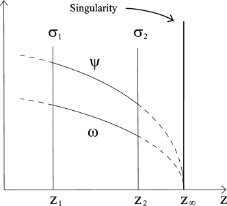
Figure 3: The figure shows the solutions of $\psi(z)$ and $\omega(z)$ for the exponential case, when the gauge $N$ constant is adopted.

The Randall-Sundrum scenario is easily obtained by letting $\alpha\rightarrow 0$. In this limit, the above solutions can be reexpressed as:

$$\psi(z) = 0,$$ (56)

$$\omega(z) = e^{-\mu Nz},$$ (57)

where $\mu=(1/4)U_{B}$. In this case, the singularities are located at infinity. Note that in this case the only degree of freedom is $N$, the radion field.

IV Low Energy Regime Expansion

We are now in a position to deduce the equations of motion governing the low energy regime. They consist in a linear expansion of the fields about the static vacuum solution found in the last section. As we shall see, these equations can be put in an integral form, allowing the construction of a systematic scheme to obtain solutions, order by order. The zeroth order solution of this expansion corresponds to the static vacuum solutions with the integration constants $\psi^{1}$ and $\psi^{2}$, and the metric $\tilde{g}_{\mu\nu}$ promoted to be space-time dependent.

IV.1 Low Energy Regime Equations

Let us develop the equations for the low energy regime. To start, assume that $\psi_{0}$, $\omega_{0}$ and $N_{0}$ are functions of $x$ and $z$ that satisfy the BPS-conditions:

$$\frac{\omega_{0}^{\prime}}{\omega_{0}} = -\frac{1}{4}N_{0}U_{B}(\psi_{0}),$$ (58)

$$\psi_{0}^{\prime} = N_{0}\frac{\partial U_{B}}{\partial\psi_{0}},$$ (59)

and let us define the bulk scalar field boundary values as $\psi_{0}^{1}=\psi_{0}(z_{1})$ and $\psi_{0}^{2}=\psi_{0}(z_{2})$ (note that they are functions of the space-time coordinate $x$). The solution for the warp factor, $\omega_{0}$, is found to be:

$$\omega_{0}(z,x)=\exp\left[-\frac{1}{4}\int_{\psi_{0}^{1}}^{\psi_{0}}\alpha^{\!-1}(\psi)\,d\psi\right],$$ (60)

where the $z$ and $x$ dependence enter through the functions $\psi_{0}^{1}(x)$ and $\psi_{0}(z,x)$ in the integration limits. It will be convenient to define the warp factor between the two branes as $\bar{\omega}=\omega_{0}(z_{2})$, or more explicitly, as:

$$\bar{\omega}(x)=\exp\left[-\frac{1}{4}\int_{\psi_{0}^{1}}^{\psi_{0}^{2}}\alpha^{\!-1}(\psi)\,d\psi\right].$$ (61)

Now, we would like to study the perturbed system about the static vacuum solution. With this purpose, let us define the following set of variables, $h_{\mu\nu}$, $\varphi$ and $\phi$, as:

$$g_{\mu\nu} = \omega_{0}^{2}\left(\tilde{g}_{\mu\nu}+h_{\mu\nu}\right),$$ (62)

$$\psi = \psi_{0}+\varphi,$$ (63)

$$N = N_{0}\,e^{\phi},$$ (64)

where $g_{\mu\nu}$, $\psi$ and $N$ satisfy the equations of motion (13), (15) and (19), taking into account the presence of matter in the branes and supersymmetry breaking terms in the potentials. Additionally, $\tilde{g}_{\mu\nu}$ depends only on the space-time coordinate $x$. Note that if there is no matter content in the branes and $u=v_{1}=v_{2}=0$, then we can take $h_{\mu\nu}=\varphi=\phi=0$, and the fields $g_{\mu\nu}$, $\psi$ and $N$ of the previous definition would correspond to the static vacuum solution discussed in the last section, with $\psi_{0}^{1}$ and $\psi_{0}^{2}$ the two constant degrees of freedom. Therefore, the functions $h_{\mu\nu}$, $\varphi$ and $\phi$ are linear deviations from the vacuum solution of the system. Since we are interested in the low energy regime, we consider the case $|h_{\mu\nu}|\ll|\tilde{g}_{\mu\nu}|$, $|\varphi|\ll|\psi_{0}|$ and $|\phi|\ll 1$. Now, if we insert these previous definitions in the equations of motion (13), (15) and (19), and neglect second order quantities in terms of $h_{\mu\nu}$, $\varphi$ and $\phi$ we obtain the equations of motion for the low energy regime. First, equation (13) leads to:

$$N_{0}U_{B}(\psi_{0})\,\tilde{g}^{\alpha\beta}h_{\alpha\beta}^{\prime}+2N_{0}\frac{\partial U_{B}}{\partial\psi_{0}}\varphi^{\prime}\qquad\quad$$

$$-N^{2}_{0}\left[2U_{0}\phi+\frac{\partial U_{0}}{\partial\psi_{0}}\varphi\right]=\frac{N_{0}^{2}}{\omega_{0}^{2}}\mathcal{X}.$$ (65)

Equation (15) leads to the 4-dimensional Einstein’s equations:

$$h_{\mu\nu}^{\prime\prime}-\tilde{g}_{\mu\nu}\tilde{g}^{\alpha\beta}h_{\alpha\beta}^{\prime\prime}$$

$$-\left[N_{0}U_{B}(\psi_{0})+\frac{\partial N_{0}}{\partial\psi_{0}}\frac{\partial U_{B}}{\partial\psi_{0}}\right](h_{\mu\nu}^{\prime}-\tilde{g}_{\mu\nu}\tilde{g}^{\alpha\beta}h_{\alpha\beta}^{\prime})$$

$$-\frac{3}{2}N_{0}U_{B}(\psi_{0})\,\phi^{\prime}\,\tilde{g}_{\mu\nu}-\frac{3}{2}N_{0}\frac{\partial U_{B}}{\partial\psi_{0}}\,\varphi^{\prime}\,\tilde{g}_{\mu\nu}$$

$$-\frac{3}{4}N_{0}^{2}\left[2U_{0}\phi+\frac{\partial U_{0}}{\partial\psi_{0}}\varphi\right]\tilde{g}_{\mu\nu}=2\frac{N_{0}^{2}}{\omega_{0}^{2}}\mathcal{Y}_{\mu\nu}.$$ (66)

And finally, equation (19) [with the help of equation (13)] leads to:

$$\varphi^{\prime\prime}-\left[N_{0}U_{B}(\psi_{0})+\frac{\partial N_{0}}{\partial\psi_{0}}\frac{\partial U_{B}}{\partial\psi_{0}}\right]\varphi^{\prime}$$

$$-N_{0}\frac{\partial U_{B}}{\partial\psi_{0}}\phi^{\prime}+\frac{1}{2}N_{0}\frac{\partial U_{B}}{\partial\psi_{0}}\tilde{g}^{\mu\nu}h_{\mu\nu}^{\prime}$$

$$-\frac{N_{0}^{2}}{2}\left[2\phi\frac{\partial U_{0}}{\partial\psi_{0}}+\frac{\partial^{2}U_{0}}{\partial\psi_{0}^{2}}\varphi\right]=\frac{N^{2}_{0}}{\omega_{0}^{2}}\left(\mathcal{Z}-\frac{1}{2}\alpha_{0}\mathcal{X}\right).$$ (67)

In the previous equations, $U_{0}=U(\psi_{0})$. Equations (65) and (66) correspond to the linearized Einstein’s equations, while equation (67) corresponds to the linearized bulk scalar field equation. In the previous set of equations we have defined, for the sake of notation, the functions $\mathcal{X}$, $\mathcal{Y}_{\mu\nu}$ and $\mathcal{Z}$, in the following way:

$$\mathcal{X} = \omega_{0}^{2}\left[(\partial\psi)^{2}-\frac{4}{3}R+u\right],$$ (68)

$$\mathcal{Y}_{\mu\nu} = G_{\mu\nu}+\frac{1}{N}\big{(}g_{\mu\nu}\Box N-\nabla_{\mu}\nabla_{\nu}N\big{)}$$ (69)

$$+\frac{3}{4}\bigg{(}\frac{1}{2}g_{\mu\nu}(\partial\psi)^{2}-\partial_{\mu}\psi\partial_{\nu}\psi+\frac{1}{2}g_{\mu\nu}u\bigg{)},\quad$$

$$\mathcal{Z} = \omega_{0}^{2}\left[\frac{1}{2}\frac{\partial u}{\partial\psi_{0}}-\frac{1}{N}g^{\mu\nu}\nabla_{\mu}(N\partial_{\nu}\psi)\right].$$ (70)

Note that in the functions $\mathcal{X}$, $\mathcal{Y}_{\mu\nu}$ and $\mathcal{Z}$, the quantities $g_{\mu\nu}$, $\psi$ and $N$ are not explicitly expanded. Their expansions can be considered in the following way:

$$\mathcal{X} = X_{0}+X,$$

$$\mathcal{Y}_{\mu\nu} = Y_{\mu\nu}^{0}+Y_{\mu\nu},$$

$$\mathcal{Z} = Z_{0}+Z,$$ (71)

where $X_{0}$, $Y_{\mu\nu}^{0}$ and $Z_{0}$ are the zeroth order terms in the expansions of $\mathcal{X}$, $\mathcal{Y}_{\mu\nu}$ and $\mathcal{Z}$ (that is, they are constructed from $\tilde{g}_{\mu\nu}$, $\psi_{0}$ and $N_{0}$) while $X$, $Y_{\mu\nu}$ and $Z$ are the terms which contain linear contributions from $h_{\mu\nu}$, $\varphi$ and $\phi$. Their specific form are given in Appendix A. We can now replace the new set of variables in the Israel matching conditions and the scalar field boundary condition. At the first brane, $\sigma_{1}$, these take the form:

$$h_{\mu\nu}^{\prime}-\tilde{g}_{\mu\nu}\tilde{g}^{\alpha\beta}h_{\alpha\beta}^{\prime}=\frac{3}{2}N_{0}U_{B}(\psi_{0})\,\phi\,\tilde{g}_{\mu\nu}\qquad$$

$$+\frac{3}{2}N_{0}\frac{\partial U_{B}}{\partial\psi_{0}}\,\varphi\,\tilde{g}_{\mu\nu}+\frac{3}{2}N_{0}v_{1}\tilde{g}_{\mu\nu}-\kappa_{5}^{2}N_{0}T_{\mu\nu}^{\,1},$$ (72)

and

$$\varphi^{\prime}=N_{0}\frac{\partial U_{B}}{\partial\psi_{0}}\phi+N_{0}\frac{\partial^{2}U_{B}}{\partial\psi_{0}^{2}}\varphi+N_{0}\frac{\partial v_{1}}{\partial\psi_{0}},$$ (73)

where, quantities like $\psi_{0}$ and $N_{0}$, not explicitly evaluated at the boundary, must be evaluated at $z=z_{1}$. Meanwhile, at the second brane, $\sigma_{2}$, the matching conditions are:

$$h_{\mu\nu}^{\prime}-\tilde{g}_{\mu\nu}\tilde{g}^{\alpha\beta}h_{\alpha\beta}^{\prime}=\frac{3}{2}N_{0}U_{B}(\psi_{0})\,\phi\,\tilde{g}_{\mu\nu}\qquad$$

$$+\frac{3}{2}N_{0}\frac{\partial U_{B}}{\partial\psi_{0}}\,\varphi\,\tilde{g}_{\mu\nu}+\frac{3}{2}N_{0}v_{2}\tilde{g}_{\mu\nu}+\kappa_{5}^{2}N_{0}T_{\mu\nu}^{\,2}\bar{\omega}_{0}^{-2},$$ (74)

and

$$\varphi^{\prime}=N_{0}\frac{\partial U_{B}}{\partial\psi_{0}}\phi+N_{0}\frac{\partial^{2}U_{B}}{\partial\psi_{0}^{2}}\varphi+N_{0}\frac{\partial v_{2}}{\partial\psi_{0}},$$ (75)

where again, quantities like $\psi_{0}$ and $N_{0}$ must be evaluated at $z=z_{2}$. Note that in the boundary conditions the new set of variables are linearly proportional to the energy-momentum tensor at the branes. In other words, deviations of the boundary conditions from the BPS-state generate the existence of fields $h_{\mu\nu}$, $\varphi$ and $\phi$ in the bulk, as expected in the low energy regime. In order to solve the equations of motion it is useful to rewrite them in the form of a set of first order differential equations in terms of the $\partial_{z}$ derivative. This can be done by defining new fields $\xi_{\mu\nu}$ and $\chi$ to be sources of the fields $h_{\mu\nu}$, $\varphi$ and $\phi$, in the following equations:

$$h_{\mu\nu}^{\prime}-\tilde{g}_{\mu\nu}\tilde{g}^{\alpha\beta}h_{\alpha\beta}^{\prime}-\frac{3}{2}N_{0}U_{B}(\psi_{0})\,\phi\,\tilde{g}_{\mu\nu}$$

$$-\frac{3}{2}N_{0}\frac{\partial U_{B}}{\partial\psi_{0}}\,\varphi\,\tilde{g}_{\mu\nu} = \xi_{\mu\nu},$$ (76)

$$\varphi^{\prime}-N_{0}\frac{\partial U_{B}}{\partial\psi_{0}}\phi-N_{0}\frac{\partial^{2}U_{B}}{\partial\psi_{0}^{2}}\varphi = \chi.$$ (77)

With these definitions of $\xi_{\mu\nu}$ and $\chi$, it is found that equations (65), (66) and (67) can be reexpressed in a much simpler way. Respectively, these equations are found to be:

$$2N_{0}\frac{\partial U_{B}}{\partial\psi_{0}}\chi-\frac{1}{3}N_{0}U_{B}(\psi_{0})\xi=\frac{N_{0}^{2}}{\omega_{0}^{2}}\mathcal{X},$$ (78)

$$\left[\frac{\omega_{0}^{4}}{N_{0}}\,\xi_{\mu\nu}\right]^{\prime}=2N_{0}\omega_{0}^{2}\mathcal{Y}_{\mu\nu},$$ (79)

$$\left[\alpha_{0}\frac{\omega_{0}^{4}}{N_{0}}\chi\right]^{\prime}=\alpha_{0}N_{0}\omega_{0}^{2}\left(\mathcal{Z}-\frac{1}{2}\alpha_{0}\mathcal{X}\right),$$ (80)

where $\xi=\tilde{g}^{\mu\nu}\xi_{\mu\nu}$. Note that the left hand sides of equations (79) and (80) consist of first order derivatives of $\xi_{\mu\nu}$ and $\chi$ in terms of $z$, while the right hand sides depends on second order derivatives in terms of the space-time coordinate $x$. The boundary values of $\xi_{\mu\nu}$ and $\chi$, at the positions of the branes, can be computed with the help of the boundary conditions (72)-(75). These are:

$$\xi_{\mu\nu}(z_{1}) = \frac{3}{2}N_{0}v_{1}\tilde{g}_{\mu\nu}-\kappa_{5}^{2}N_{0}T_{\mu\nu}^{\,1},$$ (81)

$$\chi(z_{1}) = N_{0}\frac{\partial v_{1}}{\partial\psi_{0}},$$ (82)

at position $z_{1}$, and

$$\xi_{\mu\nu}(z_{2}) = \frac{3}{2}N_{0}v_{2}\tilde{g}_{\mu\nu}+\kappa_{5}^{2}N_{0}T_{\mu\nu}^{\,2}\bar{\omega}^{-2},$$ (83)

$$\chi(z_{2}) = N_{0}\frac{\partial v_{2}}{\partial\psi_{0}},$$ (84)

at position $z_{2}$. (Recall that $\omega_{0}(z_{1})=1$ and $\omega_{0}(z_{2})=\bar{\omega}$). We should not forget at this point the additional equations for the matter content at both branes. They come from equation (40) and, with the present notation, are given by:

$$\tilde{\nabla}^{\nu}T^{1}_{\mu\nu} = 0,$$ (85)

$$\tilde{\nabla}^{\nu}T^{2}_{\mu\nu} = \frac{1}{\bar{\omega}}\left[(\tilde{\nabla}_{\mu}\bar{\omega})\tilde{g}^{\alpha\beta}T^{2}_{\alpha\beta}-2(\tilde{\nabla}^{\nu}\bar{\omega})T^{2}_{\mu\nu}\right],$$ (86)

where covariant derivatives $\tilde{\nabla}_{\mu}$ are constructed from the $\tilde{g}_{\mu\nu}$ metric. Additionally, it is worth mentioning that the projected Weyl tensor $E_{\mu\nu}$ and the loss parameter $\Delta\psi$ can be written in terms of the linear variables as:

$$E_{\mu\nu} = -\frac{\omega_{0}^{2}}{2N_{0}}\left[\xi_{\mu\nu}^{\prime}-\frac{1}{3}\tilde{g}_{\mu\nu}\tilde{g}^{\alpha\beta}\xi_{\alpha\beta}^{\prime}\right]$$ (87)

$$+\frac{1}{4}\frac{\omega_{0}^{2}}{N_{0}}U_{B}(\psi_{0})\left[\xi_{\mu\nu}-\frac{1}{3}\tilde{g}_{\mu\nu}\tilde{g}^{\alpha\beta}\xi_{\alpha\beta}\right]$$

$$-\frac{3}{8}\tilde{g}_{\mu\nu}\frac{\partial U_{B}}{\partial\psi_{0}}\frac{\chi}{N_{0}}-\frac{1}{4}\bigg{[}\frac{1}{4}g_{\mu\nu}u+\partial_{\mu}\psi\partial_{\nu}\psi$$

$$-\frac{1}{4}g_{\mu\nu}(\partial\psi)^{2}+\frac{4}{N}\nabla_{\mu}\nabla_{\nu}N\bigg{]},$$

$$\Delta\psi = \frac{1}{N_{0}}\left[\frac{\chi}{N_{0}}\right]^{\prime}.$$ (88)

One of the main features of equations (79) and (80) is that now they can be put in an integral form. That is, we can write:

$$\frac{\omega_{0}^{4}}{N_{0}}\xi_{\mu\nu}(z) = \frac{3}{2}\tilde{g}_{\mu\nu}v_{1}-\kappa_{5}^{2}T_{\mu\nu}^{\,1}$$ (89)

$$+2\int_{z_{1}}^{z}dz\,N_{0}\omega_{0}^{2}\mathcal{Y}_{\mu\nu},$$

$$\alpha_{0}\frac{\omega_{0}^{4}}{N_{0}}\chi(z) = \alpha_{0}(\psi_{0}^{1})\frac{\partial v_{1}}{\partial\psi_{0}^{1}}$$ (90)

$$+\int_{z_{1}}^{z}dz\,\alpha_{0}N_{0}\omega_{0}^{2}\left(\mathcal{Z}-\frac{1}{2}\alpha_{0}\mathcal{X}\right),$$

where we have used the boundary conditions at the position of the first brane. To further proceed we must implement a systematic expansion order by order in which the vacuum solution serves as the zeroth order solution. We develop this in the next subsection.

IV.2 Low Energy Regime Expansion

Equations (89) and (90) are two integral equations of the system, which suggest the possibility of introducing a systematic expansion about the vacuum solution, order by order. In the last subsection we saw that the matter content of the branes are sources for the linear deviations $h_{\mu\nu}$, $\varphi$ and $\phi$ on the bulk. Therefore, it is sensible to study how the bulk is affected by the matter distribution on the brane, at different scales. In this way, let us consider the following expansion for the energy-momentum tensor of the matter content on the branes, as well as for the supersymmetry breaking potentials:

$$T_{\mu\nu}^{1} = T_{\mu\nu}^{1\,(0)}+T_{\mu\nu}^{1\,(1)}+T_{\mu\nu}^{1\,(2)}+\cdots,$$ (91)

$$v_{1} = v_{1}^{(0)}+v_{1}^{(1)}+v_{1}^{(2)}+\cdots,$$ (92)

and

$$T_{\mu\nu}^{2} = T_{\mu\nu}^{2\,(0)}+T_{\mu\nu}^{2\,(1)}+T_{\mu\nu}^{2\,(2)}+\cdots,$$ (93)

$$v_{2} = v_{2}^{(0)}+v_{2}^{(1)}+v_{2}^{(2)}+\cdots.$$ (94)

The parameter of the expansion is dictated by the scale at which each term becomes relevant in the physical problem of interest. Naturally, the expansion above will induce an expansion of the source functions $\xi_{\mu\nu}$ and $\chi$, given by:

$$\xi_{\mu\nu} = \xi_{\mu\nu}^{(1)}+\xi_{\mu\nu}^{(2)}+\cdots,$$ (95)

$$\chi = \chi_{(1)}+\chi_{(2)}+\cdots,$$ (96)

in this way, the boundary conditions (81)-(84), can now be written, order by order, as:

$$\xi_{\mu\nu}^{(i+1)}(z_{1}) = \frac{3}{2}N_{0}v_{1}^{(i)}\tilde{g}_{\mu\nu}-\kappa_{5}^{2}N_{0}T_{\mu\nu}^{1\,(i)},$$ (97)

$$\chi_{(i+1)}(z_{1}) = N_{0}\frac{\partial v_{1}^{(i)}}{\partial\psi_{0}},$$ (98)

at position $z_{1}$, and

$$\xi_{\mu\nu}^{(i+1)}(z_{2}) = \frac{3}{2}N_{0}v_{2}^{(i)}\tilde{g}_{\mu\nu}+\kappa_{5}^{2}N_{0}T_{\mu\nu}^{2\,(i)}\bar{\omega}^{-2},$$ (99)

$$\chi_{(i+1)}(z_{2}) = N_{0}\frac{\partial v_{2}^{(i)}}{\partial\psi_{0}},$$ (100)

at position $z_{2}$. Note the convention whereby the indicies of the left hand side are raised by one unit in relation those on the right hand side. Continuing with the construction, we must also consider the expansion of $h_{\mu\nu}$, $\varphi$ and $\phi$:

$$h_{\mu\nu} = h_{\mu\nu}^{(1)}+h_{\mu\nu}^{(2)}+\cdots,$$ (101)

$$\varphi = \varphi_{(1)}+\varphi_{(2)}+\cdots,$$ (102)

$$\phi = \phi_{(1)}+\phi_{(2)}+\cdots.$$ (103)

They are defined to satisfy the following first order differential equations with sources $\xi_{\mu\nu}^{(i)}$ and $\chi_{(i)}$:

$$h_{\mu\nu}^{(i)}\,\!{}^{\prime}-\tilde{g}_{\mu\nu}\tilde{g}^{\alpha\beta}h_{\alpha\beta}^{(i)}\,\!{}^{\prime}-\frac{3}{2}N_{0}U_{B}(\psi_{0})\,\phi_{(i)}\,\tilde{g}_{\mu\nu}$$

$$-\frac{3}{2}N_{0}\frac{\partial U_{B}}{\partial\psi_{0}}\,\varphi_{(i)}\,\tilde{g}_{\mu\nu}=\xi_{\mu\nu}^{(i)},$$ (104)

$$\varphi_{(i)}^{\prime}-N_{0}\frac{\partial U_{B}}{\partial\psi_{0}}\phi_{(i)}-N_{0}\frac{\partial^{2}U_{B}}{\partial\psi_{0}^{2}}\varphi_{(i)}=\chi_{(i)}.$$ (105)

Finally, recall that the quantities $\mathcal{X}$, $\mathcal{Y}_{\mu\nu}$ and $\mathcal{Z}$ defined in equations (71) depend on the fields $h_{\mu\nu}$, $\varphi$ and $\phi$. Therefore, we must consider the following expansion

$$\mathcal{X} = X_{0}+X_{(1)}+X_{(2)}+\cdots,$$ (106)

$$\mathcal{Y}_{\mu\nu} = Y_{\mu\nu}^{0}+Y_{\mu\nu}^{(1)}+Y_{\mu\nu}^{(2)}+\cdots,$$ (107)

$$\mathcal{Z} = Z_{0}+Z_{(1)}+Z_{(2)}+\cdots,$$ (108)

where the index “$0$” denotes the dependence on the zeroth order quantities, $N_{0}$, $\psi_{0}$ and $\omega_{0}$, and the index $i\geq 1$ denotes quantities that depend linearly on $h_{\mu\nu}^{(i)}$, $\varphi_{(i)}$ and $\phi_{(i)}$. The precise form of the expanded functions $X_{(i)}$, $Y^{(i)}_{\mu\nu}$ and $Z_{(i)}$ are shown in Appendix A. Observe that it follows from equations (85) and (86) that the $i$-th order term, $T_{\mu\nu}^{a\,(i)}$, in the expansion of the energy momentum tensor for the matter living in the brane, satisfies the following conservation relation:

$$\tilde{\nabla}^{\nu}T^{1\,(i)}_{\mu\nu} = 0,$$ (109)

$$\tilde{\nabla}^{\nu}T^{2\,(i)}_{\mu\nu} = \frac{1}{\bar{\omega}}\big{[}(\tilde{\nabla}_{\mu}\bar{\omega})\tilde{g}^{\alpha\beta}T^{2\,(i)}_{\alpha\beta}$$ (110)

$$-2(\tilde{\nabla}^{\nu}\bar{\omega})T^{2\,(i)}_{\mu\nu}\big{]}.$$

With all these previous definitions we can now cast the equations of motion in the following way:

$$2\frac{\partial U_{B}}{\partial\psi_{0}}\chi_{(i+1)}-\frac{1}{3}U_{B}(\psi_{0})\xi_{(i+1)}=\frac{N_{0}}{\omega_{0}^{2}}X_{(i)},$$ (111)

$$\left[\frac{\omega_{0}^{4}}{N_{0}}\xi_{\mu\nu}^{(i+1)}\right]^{\prime}=2N_{0}\omega_{0}^{2}Y^{(i)}_{\mu\nu},$$ (112)

$$\left[\alpha_{0}\,\frac{\omega_{0}^{4}}{N_{0}}\,\chi_{(i+1)}\right]^{\prime}=\alpha_{0}N_{0}\omega_{0}^{2}\left(Z_{(i)}-\frac{1}{2}\alpha_{0}X_{(i)}\right).$$ (113)

This last set of equations shows the desired low energy regime expansion. It states that $\xi_{\mu\nu}^{(i+1)}$ and $\chi_{(i+1)}$ can be solved in terms of the lower order quantities $\mathcal{X}_{(i)}$, $\mathcal{Y}^{(i)}_{\mu\nu}$ and $\mathcal{Z}_{(i)}$. At the same time, the functions $\mathcal{X}_{(i)}$, $\mathcal{Y}^{(i)}_{\mu\nu}$ and $\mathcal{Z}_{(i)}$ can be solved in terms of $\xi_{\mu\nu}^{(i)}$ and $\chi_{(i)}$, as evident from their definitions. Note that the former means that we can compute $E_{\mu\nu}$ and $\Delta\psi$ to any desired order, as indicated by equations (87) and (88). In this way, starting with the zeroth order solutions $\psi_{0}$, $N_{0}$ and $\tilde{g}_{\mu\nu}$, we can arrive at any desired order for the full solutions to the bulk equations $\psi$, $N$ and $g_{\mu\nu}$. The present method is similar to the one introduced by Kanno and Soda for the Randall-Sundrum model Kanno-Soda 1 ; Kanno-Soda 2 as well as to other schemes Kobayashi-Koyama ; Mukohyama-Kofman ; Mukohyama-Coley ; Kanno-Soda 3 for dilatonic brane-worlds.

We mentioned that the expansion parameter was dictated by the scale at which each term of the energy-momentum tensor expansion was relevant for the physical process of interest. In terms of the bulk quantities, one finds that the effect on the variation of the scale in the extra-dimensional direction is related to the variation of the scales in the space-time direction as follows:

$$h_{(i+1)}^{\prime\prime}\simeq\frac{N_{0}^{2}}{\omega_{0}^{2}}\Box h_{(i)},$$ (114)

That is, second derivatives of the $(i+1)$-th order variables in terms of $z$ are of the same order as the second order derivatives of the $i$-th order variables in terms of space-time coordinates.

As in the previous case, we can rewrite equations (112) and (113) in an integral form:

$$\frac{\omega_{0}^{4}}{N_{0}}\xi^{(i+1)}_{\mu\nu}=\frac{3}{2}\tilde{g}_{\mu\nu}v_{1}-\kappa_{5}^{2}T_{\mu\nu}^{\,1}$$ (115)

$${}+2\int_{z_{1}}^{z}\!\!\!dzN_{0}\omega_{0}^{2}Y^{(i)}_{\mu\nu},$$

$$\alpha_{0}\frac{\omega_{0}^{4}}{N_{0}}\chi_{(i+1)}=\alpha_{1}\frac{\partial v_{1}}{\partial\psi_{0}^{1}}$$ (116)

$${}+\int_{z_{1}}^{z}\!\!\!dz\alpha_{0}N_{0}\omega_{0}^{2}\left(Z_{(i)}-\frac{1}{2}\alpha_{0}X_{(i)}\right).$$

This form of the expanded equations of motion are highly relevant; they are the basis for the derivation of the effective theory developed in the next section.

Summarizing, in this section we have developed an expansion procedure to solve the entire theory in a systematic form. As we said, to solve this system of equations we need to know the form of the zeroth order moduli fields $\psi^{1}_{0}$ and $\psi^{2}_{0}$, and the metric $\tilde{g}_{\mu\nu}$ and, therefore, an effective theory for these fields is required. In the following section, we are going to deduce the 4-dimensional equations of motion governing these functions, as well as those for higher order terms in the expansion.

V Four Dimensional Effective Theory

In the previous section we have shown how to construct the low energy regime as a consistent expansion. In this section we see how to define the four-dimensional effective theory at the position of the branes starting from the expansion above. Concordant with the expansion, the effective theory must be defined order by order.

V.1 General Case

The effective equations governing the variables at the $i$-th order can be obtained by evaluating the integral equations (115) and (116) at $z=z_{2}$. In other words, the $i$-th order equations are given by:

$$2\int_{z_{1}}^{z_{2}}\!\!\!dz\,N_{0}\omega_{0}^{2}Y^{(i)}_{\mu\nu}=\frac{3}{2}\big{[}\bar{\omega}^{4}v_{2}^{(i)}-v_{1}^{(i)}\big{]}\tilde{g}_{\mu\nu}$$

$$+\kappa_{5}^{2}\left[T_{\mu\nu}^{2\,(i)}\bar{\omega}^{2}+T_{\mu\nu}^{1\,(i)}\right],$$ (117)

$$\int_{z_{1}}^{z_{2}}\!\!\!dz\,\alpha_{0}N_{0}\omega_{0}^{2}\bigg{(}Z_{(i)}-\frac{1}{2}\alpha_{0}X_{(i)}\bigg{)}=\alpha_{2}\bar{\omega}^{4}\frac{\partial v_{2}^{(i)}}{\partial\psi_{0}^{2}}$$

$$-\alpha_{1}\frac{\partial v_{1}^{(i)}}{\partial\psi_{0}^{1}},$$ (118)

Additionally, another equation can be obtained by evaluating equation (111) at the boundary position $z_{1}$. The resulting equation is:

$$X_{(i)}(z_{1}) = 2\frac{\partial U_{B}}{\partial\psi_{0}^{1}}\frac{\partial v_{1}^{(i)}}{\partial\psi_{0}^{1}}-2U_{B}(\psi_{0}^{1})v_{1}^{(i)}$$ (119)

$$+\frac{\kappa_{5}^{2}}{3}U_{B}(\psi_{0}^{1})\,\tilde{g}^{\mu\nu}T^{1\,(i)}_{\mu\nu}.$$

Note that a similar equation would have been obtained by evaluating (111) at the boundary position $z_{2}$, however, this would not give a new equation of motion. Equations (117)-(119) are the desired equations of the 4-dimensional effective theory. Solving these equations for the $i$-th order variables allows us to obtain the effective equations for the $(i+1)$-th order variables, after correctly integrating (104) and (105). The form in which equations (117)-(119) are presented is, at this level, abstract and it is difficult to appreciate the effective theory in more familiar terms. In the next subsection we analyze in detail the effective theory at the zeroth order in the expansion ($i=0$).

V.2 Zeroth Order Effective Theory

It will be particularly interesting to analyze the form of the effective equations at the zeroth order in more detail. In this case the metric at the first and second branes are conformally related. In terms of the treatment developed in the previous section, the effective theory is:

$$\int_{z_{1}}^{z_{2}}\!\!\!\!\!dz\,N_{0}\omega_{0}^{2}Y^{0}_{\mu\nu}=\frac{3}{4}\tilde{g}_{\mu\nu}\left[\bar{\omega}^{4}v_{2}^{0}-v_{1}^{(0)}\right]$$

$$+\frac{\kappa_{5}^{2}}{2}\left[T_{\mu\nu}^{2\,(0)}\bar{\omega}^{2}+T_{\mu\nu}^{1\,(0)}\right],$$ (120)

$$\int_{z_{1}}^{z_{2}}\!\!\!\!\!dz\,\alpha_{0}N_{0}\omega_{0}^{2}\bigg{(}Z_{0}-\frac{1}{2}\alpha_{0}X_{0}\bigg{)}=\alpha_{2}\bar{\omega}^{4}\frac{\partial v_{2}^{(0)}}{\partial\psi^{2}_{0}}$$

$$-\alpha_{1}\frac{\partial v_{1}^{(0)}}{\partial\psi^{1}_{0}},$$ (121)

$$X_{0}(z_{1})=2\frac{\partial U_{B}}{\partial\psi^{1}_{0}}\frac{\partial v_{1}^{(0)}}{\partial\psi^{1}_{0}}-2U_{B}(\psi^{1}_{0})v_{1}^{(0)}$$

$$+\frac{\kappa_{5}^{2}}{3}U_{B}(\psi^{1}_{0})\,\tilde{g}^{\mu\nu}T^{1\,(0)}_{\mu\nu}.$$ (122)

In the following, we shall omit the “$0$” index denoting the zeroth order terms. To rewrite this theory in more familiar terms, we need to integrate the terms on the left hand side of equations (120) and (121). In order to do this we need to evaluate the terms at the boundaries. Hence it is particularly useful to express the theory in terms of the moduli fields $\psi^{1}$ and $\psi^{2}$. It is then possible to obtain the following effective theory (Appendix B shows how to derive the next results). The Einstein’s equations, obtained from (120), are found to be:

$$\Omega^{2}\tilde{G}_{\mu\nu}=-\tilde{g}_{\mu\nu}\tilde{\Box}\,\Omega^{2}+\tilde{\nabla}_{\mu}\tilde{\nabla}_{\nu}\Omega^{2}\qquad\qquad\qquad$$

$$-\frac{3}{4}\gamma_{ab}\bigg{(}\frac{1}{2}\tilde{g}_{\mu\nu}\tilde{g}^{\alpha\beta}\partial_{\alpha}\psi^{a}\partial_{\beta}\psi^{b}-\partial_{\mu}\psi^{a}\partial_{\nu}\psi^{b}\bigg{)}$$

$$+\frac{k\kappa_{5}^{2}}{2}\left[\bar{\omega}^{2}T_{\mu\nu}^{2}+T_{\mu\nu}^{1}\right]-\frac{3}{4}\tilde{g}_{\mu\nu}V,$$ (123)

while the moduli fields equations, obtained from equations (120) and (122), are found to be:

$$\tilde{\Box}\psi^{a} = -\tilde{g}^{\mu\nu}\gamma^{a}_{bc}\partial_{\mu}\psi^{b}\partial_{\nu}\psi^{c}+\frac{1}{2}\gamma^{ac}\frac{\partial V}{\partial\psi^{c}}$$ (124)

$$-\frac{2}{3}\gamma^{ac}\frac{\partial\Omega^{2}}{\partial\psi^{c}}\tilde{R}-\frac{2}{3}k\kappa_{5}^{2}\bar{\omega}\gamma^{ac}\frac{\partial\bar{\omega}}{\partial\psi^{c}}\tilde{g}^{\mu\nu}T^{2}_{\mu\nu}.\qquad$$

In the previous expressions, the index $a$ labels the positions $1$ and $2$. Additionally, note the presence of a conformal factor $\Omega^{2}$ in front of the Einstein’s tensor $G_{\mu\nu}$, given by:

$$\Omega^{2}=k\int_{\psi^{1}}^{\psi^{2}}\!\!\!\!\!d\psi\left(\frac{\partial U_{B}}{\partial\psi}\right)^{-1}\!\!\!\omega^{2},$$ (125)

where $\omega$ is given by equation (47). The coefficient $k$ is an arbitrary positive constant with dimensions of inverse length, which has been incorporated to make $\Omega^{2}$ dimensionless. The symmetric matrix $\gamma_{ab}$ is a function of the moduli fields, that can be regarded as the metric of the space spanned by the moduli in a sigma model approach, with $\gamma^{ab}$ its inverse. The elements of $\gamma_{ab}$ are given by:

$$\gamma_{11} = \alpha_{1}^{-2}\left[\frac{k}{U_{B}(\psi^{1})}-\frac{1}{2}\Omega^{2}\right],$$ (126)

$$\gamma_{22} = \alpha_{2}^{-2}\frac{\bar{\omega}^{2}k}{U_{B}(\psi^{2})},$$ (127)

$$\gamma_{12} = -\alpha_{1}^{-1}\alpha_{2}^{-1}\frac{\bar{\omega}^{2}k}{U_{B}(\psi^{2})},$$ (128)

with $\gamma_{21}=\gamma_{12}$. Associated with the above metric, we have defined a set of connections $\gamma^{a}_{bc}$. These are given by:

$$\gamma^{a}_{bc}=\frac{1}{2}\gamma^{ad}\left[\frac{\partial\gamma_{bd}}{\partial\psi^{c}}+\frac{\partial\gamma_{dc}}{\partial\psi^{b}}-\frac{\partial\gamma_{bc}}{\partial\psi^{d}}\right].$$ (129)

Finally, we have also defined an effective potential $V$ which depends linearly on the supersymmetry breaking potentials $u$, $v_{1}$ and $v_{2}$. This is defined as:

$$V=\frac{k}{2}\int^{\psi^{2}}_{\psi^{1}}\!\!\!\!\!d\psi\left(\frac{\partial U_{B}}{\partial\psi}\right)^{-1}\!\!\!\omega^{4}\,u-2k\left[\bar{\omega}^{4}v_{2}-v_{1}\right].$$ (130)

Finally, we can not forget the matter conservation relations. These take the form:

$$\tilde{\nabla}^{\nu}T^{1}_{\mu\nu} = 0,$$ (131)

$$\tilde{\nabla}^{\nu}T^{2}_{\mu\nu} = \frac{1}{\bar{\omega}}\big{[}(\tilde{\nabla}_{\mu}\bar{\omega})\tilde{g}^{\alpha\beta}T^{2}_{\alpha\beta}-2(\tilde{\nabla}^{\nu}\bar{\omega})T^{2}_{\mu\nu}\big{]}.$$ (132)

The fact that the energy-momentum tensor of the second brane does not respect the standard matter conservation relation is due to the frame chosen to describe the system.

The generic form of the theory displayed by equations (123) and (124) is of a bi-scalar tensor theory of gravity, with the two scalar degrees given by $\psi^{1}$ and $\psi^{2}$. The above set of equations can be obtained from the following action:

$$S = \frac{1}{k\kappa_{5}^{2}}\int d^{4}x\sqrt{-\tilde{g}}\bigg{[}\Omega^{2}\tilde{R}-\frac{3}{4}\tilde{g}^{\mu\nu}\gamma_{ab}\partial_{\mu}\psi^{a}\partial_{\nu}\psi^{b}-\frac{3}{4}V\bigg{]}$$ (133)

$$+S_{1}[\Psi_{1},\tilde{g}_{\mu\nu}]+S_{2}[\Psi_{2},\bar{\omega}^{2}\tilde{g}_{\mu\nu}],\qquad$$

Equation (133) is an important result. It can be shown that the effective action (133) corresponds to the moduli-space approximation prep , where the relevant fields of the theory are just simply the free degrees of freedom of the vacuum theory, promoted to be space-time dependent fields. A relevant aspect of this theory, is that the equation of motion for a moduli field $\psi^{a}$ will depend linearly on the trace of the energy-momentum tensor of the brane $a$ but not on the one belonging to the opposite brane. More precisely, it can be shown that (124) has the form:

$$\tilde{\Box}\psi^{1} = -\frac{k\kappa_{5}}{6}\frac{\partial U_{B}}{\partial\psi^{1}}\tilde{g}^{\mu\nu}T^{1}_{\mu\nu}+\cdots,$$ (134)

$$\tilde{\Box}\psi^{2} = +\frac{k\kappa_{5}}{6}\frac{\partial U_{B}}{\partial\psi^{2}}\bar{\omega}^{-2}\tilde{g}^{\mu\nu}T^{2}_{\mu\nu}+\cdots.$$ (135)

This means that, in the low energy regime, the moduli fields are driven by the matter content of the branes (recall that the moduli are parameterizing the positions of the branes). This behaviour of the moduli fields is independent of the frame choice (see next subsection).

V.3 Einstein’s Frame

Note that in equation (133) the Newton’s constant depends on the moduli fields. This theory can be rewritten in the Einstein frame where the Newton’s constant is independent of the moduli. Considering the conformal transformation:

$$\tilde{g}_{\mu\nu}\rightarrow g_{\mu\nu}=\Omega^{2}\tilde{g}_{\mu\nu},$$ (136)

we are then left with the following action

$$S = \frac{1}{k\kappa_{5}^{2}}\int d^{4}x\sqrt{-g}\bigg{[}R-\frac{3}{4}g^{\mu\nu}\gamma_{ab}\partial_{\mu}\psi^{a}\partial_{\nu}\psi^{b}-\frac{3}{4}V\bigg{]}$$ (137)

$$+S_{1}[\Psi_{1},A_{1}^{2}g_{\mu\nu}]+S_{2}[\Psi_{2},A_{2}^{2}g_{\mu\nu}],$$

where now the sigma model metric $\gamma_{ab}$ is given by:

$$\gamma_{11} = 2\alpha_{1}^{-2}\frac{k^{2}A_{1}^{4}}{U_{B}^{2}(\psi^{1})}\bigg{[}1-\frac{1}{2k}U_{B}(\psi^{1})A_{1}^{-2}\bigg{]},$$ (138)

$$\gamma_{22} = 2\alpha_{2}^{-2}\frac{k^{2}A_{2}^{4}}{U_{B}^{2}(\psi^{2})}\bigg{[}1+\frac{1}{2k}U_{B}(\psi^{2})A_{2}^{-2}\bigg{]},$$ (139)

$$\gamma_{12} = -2\alpha_{1}\alpha_{2}\frac{k^{2}A_{1}^{2}A_{2}^{2}}{U_{B}(\psi^{1})U_{B}(\psi^{2})}.$$ (140)

As usual, $\gamma^{ab}$ is the inverse of $\gamma_{ab}$, and $\gamma^{c}_{ab}$ are the connections. It is possible to show that $\gamma_{ab}$ is a positive definite metric. To work in this frame is particularly useful and simple. Additionally, we have defined the quantities $A_{1}$ and $A_{2}$ (which are functions of the moduli) to be:

$$A_{1}^{-2} = \Omega^{2}$$ (141)

$$= k\!\!\int_{\psi^{1}}^{\psi^{2}}\!\!\!\!\!d\psi\left(\frac{\partial U_{B}}{\partial\psi}\right)^{\!\!-1}\!\!\!\!\!\exp\left[-\frac{1}{2}\int_{\psi^{1}}^{\psi}\!\!\!\!\alpha^{-1}d\psi\right],\qquad$$

$$A_{2}^{-2} = \Omega^{2}\bar{\omega}^{-2}$$ (142)

$$= k\!\!\int_{\psi^{1}}^{\psi^{2}}\!\!\!\!\!d\psi\left(\frac{\partial U_{B}}{\partial\psi}\right)^{\!\!-1}\!\!\!\!\!\exp\left[-\frac{1}{2}\int_{\psi^{2}}^{\psi}\!\!\!\!\alpha^{-1}d\psi\right].\qquad$$

Also, the potential $V$ is now found to be:

$$V = \frac{k}{2}\Omega^{-4}\int^{\psi^{2}}_{\psi^{1}}\!\!\!\!\!d\psi\left(\frac{\partial U_{B}}{\partial\psi}\right)^{-1}\!\!\!\omega^{4}\,u$$ (143)

$$-2k\left[A_{2}^{4}v_{2}-A_{1}^{4}v_{1}\right].$$

The present form of the theory, can be further worked out to put the sigma model in a diagonal form with the redefinition of the moduli fields. However, in the present work we shall continue with the theory in the current notation. Let us finish this section by expressing the equations of motion in the Einstein frame. The Einstein’s equations are:

$$G_{\mu\nu} = -\frac{3}{4}\gamma_{ab}\bigg{(}\frac{1}{2}g_{\mu\nu}g^{\alpha\beta}\partial_{\alpha}\psi^{a}\partial_{\beta}\psi^{b}-\partial_{\mu}\psi^{a}\partial_{\nu}\psi^{b}\bigg{)}$$ (144)

$$+\frac{k\kappa_{5}^{2}}{2}\left[A_{2}^{2}T_{\mu\nu}^{2}+A_{1}^{2}T_{\mu\nu}^{1}\right]-\frac{3}{4}g_{\mu\nu}V,$$

and the moduli fields’ equations are:

$$\Box\psi^{1} = -g^{\mu\nu}\gamma^{1}_{bc}(\partial_{\mu}\psi^{b})(\partial_{\nu}\psi^{c})+\frac{1}{2}\gamma^{1c}\frac{\partial V}{\partial\psi^{c}}$$ (145)

$$-\frac{k\kappa_{5}^{2}}{6}\frac{\partial U_{B}}{\partial\psi^{1}}A_{1}^{2}\,g^{\mu\nu}T^{\,1}_{\mu\nu},$$

$$\Box\psi^{2} = -g^{\mu\nu}\gamma^{2}_{bc}(\partial_{\mu}\psi^{b})(\partial_{\nu}\psi^{c})+\frac{1}{2}\gamma^{2c}\frac{\partial V}{\partial\psi^{c}}$$ (146)

$$+\frac{k\kappa_{5}^{2}}{6}\frac{\partial U_{B}}{\partial\psi^{2}}A_{2}^{2}\,g^{\mu\nu}T^{\,2}_{\mu\nu}.$$

Additionally, the matter conservation relations now read:

$$\nabla^{\nu}T^{1}_{\mu\nu} = \frac{1}{A_{1}}\big{[}(\nabla_{\mu}A_{1})g^{\alpha\beta}T^{1}_{\alpha\beta}-2(\nabla^{\nu}A_{1})T^{1}_{\mu\nu}\big{]},$$ (147)

$$\nabla^{\nu}T^{2}_{\mu\nu} = \frac{1}{A_{2}}\big{[}(\nabla_{\mu}A_{2})g^{\alpha\beta}T^{2}_{\alpha\beta}-2(\nabla^{\nu}A_{2})T^{2}_{\mu\nu}\big{]}.\quad\quad$$ (148)

In the next sections, we are going to study this theory in more detail, analyzing a few examples (including the Randall-Sundrum case) and studying the cosmological evolution of the moduli for late cosmological eras. We shall pay special attention to the observational constraints that can be imposed on this model.

V.4 A Few Examples

In this subsection we shall briefly analyze two well known cases, namely, the exponential case $U_{B}(\psi)=V_{0}e^{\alpha\psi}$, and the Randall-Sundrum case, which can be derived as particular cases of the formalism described above.

V.4.1 Exponential Case

This case is particularly simple, and has been studied in detail in several previous works Davis & Brax ; Csaki etal ; Youm ; Flanagan etal 2 ; DeWolfe etal ; Br-CvdB-ACD-Rh ; Kobayashi-Koyama . The potential to consider is $U_{B}(\psi)=V_{0}e^{\alpha\psi}$, with $\alpha$ being a constant parameter of the theory. Here, it is possible (and convenient) to parameterize the theory using a new set of fields. Let us assume that $V_{0}>0$ and consider the following transformations:

$$e^{2\Phi_{1}}\cosh^{2}\Phi_{2} = \frac{2}{1+2\alpha^{2}}e^{-(1+2\alpha^{2})\psi^{1}/2\alpha},$$

$$e^{2\Phi_{1}}\sinh^{2}\Phi_{2} = \frac{2}{1+2\alpha^{2}}e^{-(1+2\alpha^{2})\psi^{2}/2\alpha}.$$ (149)

If $V_{0}<0$ then we should interchange $\psi^{1}$ and $\psi^{2}$ in the previous definition of $\Phi_{1}$ and $\Phi_{2}$. Inserting this notation back in the theory, it is possible to obtain the following effective action:

$$S = \frac{1}{k\kappa_{5}^{2}}\int d^{4}x\sqrt{-g}\bigg{[}R-\frac{12\alpha^{2}}{1+2\alpha^{2}}(\partial\Phi_{1})^{2}$$ (150)

$$-\frac{6}{1+2\alpha^{2}}(\partial\Phi_{2})^{2}-\frac{3}{4}V\bigg{]}$$

$$+S_{1}[\Psi_{1},A_{1}^{2}g_{\mu\nu}]+S_{2}[\Psi_{2},A_{2}^{2}g_{\mu\nu}],$$

where now the coefficients $A_{1}$ and $A_{2}$ are functions of the fields $\Phi_{1}$ and $\Phi_{2}$, given by:

$$A_{1}^{2} = e^{-2\Phi_{1}}\frac{V_{0}}{k}\!\left[\frac{1}{2}(1+2\alpha^{2})e^{2\Phi_{1}}\cosh^{2}\Phi_{2}\right]^{\frac{1}{1+2\alpha^{2}}},$$

$$A_{2}^{2} = e^{-2\Phi_{1}}\frac{V_{0}}{k}\!\left[\frac{1}{2}(1+2\alpha^{2})e^{2\Phi_{1}}\sinh^{2}\Phi_{2}\right]^{\frac{1}{1+2\alpha^{2}}}.\qquad$$ (151)

This form of the theory was already obtained in Br-CvdB-ACD-Rh , in the moduli-space approximation approach, and extensive analysis to it have been made.

V.4.2 Randall Sundrum Case

Finally, it is also instructive to examine the equations for the Randall-Sundrum case. This can be obtained as a limiting case of the previous example, by letting $\alpha\rightarrow 0$. The only field surviving the limiting process is $\Phi_{2}$, and the effective action is:

$$S = \frac{1}{k\kappa_{5}^{2}}\int d^{4}x\sqrt{-g}\bigg{[}R-6(\partial\Phi_{2})^{2}-\frac{3}{4}V\bigg{]}$$ (152)

$$+S_{1}[\Psi_{1},A_{1}^{2}g_{\mu\nu}]+S_{2}[\Psi_{2},A_{2}^{2}g_{\mu\nu}],$$

where now the coefficients $A_{1}$ and $A_{2}$ are functions of the field $\Phi_{2}$ alone, and are given by:

$$A_{1}^{2} = \frac{V_{0}}{2k}\cosh^{2}\Phi_{2},$$

$$A_{2}^{2} = \frac{V_{0}}{2k}\sinh^{2}\Phi_{2}.\qquad$$ (153)

In this case, however, the field is not directly coupled to matter.

VI Late-Time Cosmology

A simple and important application of the formalism developed above is the study of cosmological solutions for the most recent epoch of the Universe. In simple terms, current observations reveal that the moduli fields are not relevant for the present evolution of the universe and their dynamics is strongly suppressed. In this section we shall analyze the possibility of stabilizing the moduli fields $\psi^{1}$ and $\psi^{2}$. Interestingly, it will be found that, in order to stabilize the system, constraints must be placed on the global configurations of branes, particularly, on the class of possible potentials and also on the position of the branes with respect to the background.

VI.1 Cosmological Equations

Let us derive the cosmological equations of motion of the present system, valid for a flat, homogeneous and isotropic Universe. We can derive the equations using the flat Friedmann-Robertson-Walker (FRW) metric:

$$ds^{2}=g_{\mu\nu}dx^{\mu}dx^{\nu}=-dt^{2}+a^{2}(t)\delta_{ij}dx^{i}dx^{j}.$$ (154)

Here, $g_{\mu\nu}$ corresponds to the Einstein’s frame metric, conformally related to the physical metric, $\tilde{g}_{\mu\nu}$, of the brane frame. Using the metric (154), jointly with the effective action (137), we are left with the following Friedmann equations:

$$\frac{\ddot{a}}{a} = -\frac{k\kappa_{5}}{12}A_{1}^{4}(\rho_{1}+3p_{1})-\frac{k\kappa_{5}}{12}A_{2}^{4}(\rho_{2}+3p_{2})$$ (155)

$$-\frac{1}{4}\gamma_{ab}\dot{\psi}^{a}\dot{\psi}^{b}+\frac{1}{4}V,$$

$$H^{2} = \frac{k\kappa_{5}}{6}A_{1}^{4}\rho_{1}+\frac{k\kappa_{5}}{6}A_{2}^{4}\rho_{2}+\frac{1}{8}\gamma_{ab}\dot{\psi}^{a}\dot{\psi}^{b}$$ (156)

$$+\frac{1}{4}V,$$

where $V$ is given in equation (143) and $H=\dot{a}/a$ is the Hubble parameter. The moduli fields equations, on the other hand, are given by:

$$\ddot{\psi}^{1}+3H\dot{\psi}^{1} = -\gamma_{ab}^{1}\dot{\psi}^{a}\dot{\psi}^{b}-\frac{1}{2}\gamma^{1c}\frac{\partial V}{\partial\psi^{c}}$$ (157)

$$-\frac{1}{6}k\kappa_{5}^{2}\frac{\partial U_{B}}{\partial\psi^{1}}A_{1}^{4}(\rho_{1}-3p_{1}),$$

$$\ddot{\psi}^{2}+3H\dot{\psi}^{2} = -\gamma_{ab}^{2}\dot{\psi}^{a}\dot{\psi}^{b}-\frac{1}{2}\gamma^{2c}\frac{\partial V}{\partial\psi^{c}}$$ (158)

$$+\frac{1}{6}k\kappa_{5}^{2}\frac{\partial U_{B}}{\partial\psi^{2}}A_{2}^{4}(\rho_{2}-3p_{2}).$$

Additionally, the matter conservation relations can be read as:

$$\dot{\rho}_{1}+3H(\rho_{1}+p_{1}) = -3\frac{\dot{A}_{1}}{A_{1}}(\rho_{1}+p_{1}),$$ (159)

$$\dot{\rho}_{2}+3H(\rho_{2}+p_{2}) = -3\frac{\dot{A}_{2}}{A_{2}}(\rho_{2}+p_{2}).$$ (160)

The above set of equations are the corresponding equations of motion describing the cosmological behaviour of the brane system. Since the sigma-model metric is positive definite, the moduli fields are not going to result in an accelerating universe. Thus, in the present context, the only way to obtain an accelerating universe is to consider supersymmetry breaking potentials. A more detailed analysis of this system, taking into account the full dependence on the extra kinetic terms coming from the sigma model formulation is complicated, and shall be omitted in the present work. However, since we are interested mostly in the low energy regime of branes, we shall study the case in which the moduli are slowly evolving compared to the Hubble parameter. We examine this in the next subsection.

VI.2 Late-Time Cosmology

Let us consider the case in which the moduli fields are slowly evolving compared with the Hubble parameter, that is $|\dot{\psi}^{1}|,|\dot{\psi}^{2}|\ll H$, and that the supersymmetry breaking potentials are such that $u,v_{1},v_{2}=0$. Then, the Friedmann equations of the system are:

$$\frac{\ddot{a}}{a} = -\frac{k\kappa_{5}}{12}A_{1}^{4}(\rho_{1}+3p_{1})-\frac{k\kappa_{5}}{12}A_{2}^{4}(\rho_{2}+3p_{2}),\quad\,$$ (161)

$$H^{2} = \frac{k\kappa_{5}}{6}A_{1}^{4}\rho_{1}+\frac{k\kappa_{5}}{6}A_{2}^{4}\rho_{2}.$$ (162)

The moduli fields equations, on the other hand, are given by:

$$\ddot{\psi}^{1}+3H\dot{\psi}^{1} = -\frac{1}{6}k\kappa_{5}^{2}\frac{\partial U_{B}}{\partial\psi^{1}}A_{1}^{4}(\rho_{1}-3p_{1}),$$ (163)

$$\ddot{\psi}^{2}+3H\dot{\psi}^{2} = +\frac{1}{6}k\kappa_{5}^{2}\frac{\partial U_{B}}{\partial\psi^{2}}A_{2}^{4}(\rho_{2}-3p_{2}).$$ (164)

And the matter conservation relations can now be written as:

$$\dot{\rho}_{1}+3H(\rho_{1}+p_{1}) = 0,$$ (165)

$$\dot{\rho}_{2}+3H(\rho_{2}+p_{2}) = 0.$$ (166)

It is possible to appreciate that the moduli fields are driven by the matter content of the branes, while the evolution of the Universe remains unaffected by the moduli. In particular, if the universe is matter dominated, then there is an attractor for the moduli towards the extremes of the supersymmetric potential $U_{B}$. To be more precise, $\psi^{1}$ will be attracted to the minimum of $U_{B}$, while $\psi^{2}$ will be attracted to the maximum of $U_{B}$. This is sketched in Figure 4.

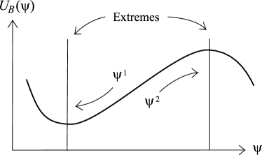
Figure 4: The figure shows the case when the branes are matter dominated. The moduli fields $\psi^{1}$ and $\psi^{2}$ are driven to the minimum and maximum of the superpotential $U_{B}$, respectively.

It is therefore sensible to assume that the present state of the Universe is very close to this configuration, where the potential is being extremize by the moduli. In the next subsection we assume that this is the case in order to place observational constraints on the model.

VI.3 Observational Constraints

We now turn to the task of placing observational bounds on the theory. In the last subsection we observed that the branes are cosmologically driven by the matter content in them. In particular, the evolution of the moduli is such that they extremize the value of the supersymmetric potential $U_{B}$. Therefore we expect that at late cosmological eras, such as the present era, the branes are far apart and their tensions nearly at their extreme values. This corresponds to an interesting global condition on the configuration of the system, however, it can be constrained by current observations. More precisely, the measurement of the Post Newtonian Eddington coefficient $\gamma$ is constrained by the Very Long Baseline Interferometry measurements of the deflection of radio waves by the Sun to be $3.8\ 10^{-4}>1-\gamma>-2.6\ 10^{-4}$ at $68\%$ confidence level Eubanks ; Will . The parameter $\gamma$ is defined as:

$$1-\gamma=2\frac{\eta^{2}}{1+\eta^{2}}\simeq 2\eta^{2},$$ (167)

where $\eta^{2}=\gamma^{ab}\,\eta_{a}\eta_{b}$, and $\eta_{a}$ is defined as:

$$\eta_{a}=\frac{1}{A_{1}}\frac{\partial A_{1}}{\partial\psi^{a}}.$$ (168)

Observe that $\eta_{a}$ is constructed from $A_{1}$, which is the factor that appears in the action for the matter content at the $\sigma_{1}$ brane. This is because we are assuming, without loss of generality, that we are performing measurements from the $\sigma_{1}$ brane. The quantity $\eta^{2}$ can be computed exactly:

$$\eta^{2}=\frac{1}{8}\left[1-\frac{1}{2k}U_{B}(\psi^{1})A_{1}^{-2}\right].$$ (169)

Then, we finally obtain:

$$1-\gamma\simeq\frac{2}{3}\left[1-\frac{1}{2k}U_{B}(\psi^{1})A_{1}^{-2}\right].$$ (170)

(Note that this result is independent of $k$). Recall that $A_{1}$ is related to an integral over the entire bulk. This is a very important result: observational measurements constrain the global configuration of the brane system. For example, we can compute the $\gamma$ parameter for the exponential potential. In this case, we obtain:

$$1-\gamma \simeq \frac{4}{3}\frac{\alpha^{2}}{1+2\alpha^{2}}$$ (171)

$$+\frac{2}{3}\frac{1}{1+2\alpha^{2}}e^{(1+2\alpha^{2})(\psi^{1}-\psi^{2})/2\alpha},$$

which agrees with earlier computations Br-CvdB-ACD-Rh . If the branes are such that the moduli are extremizing the potential $U_{B}$, then we have $\alpha(\psi^{2}-\psi^{1})\rightarrow+\infty$, and the second term will disappear in (171). Then, we end up with a constraint on $\alpha$, the parameter of the model:

$$1-\gamma \simeq \frac{4}{3}\frac{\alpha^{2}}{1+2\alpha^{2}},$$ (172)

which gives $|\alpha|<10^{-2}$. Interestingly, this bound does not affect the global configuration of the brane, but only the parameter of the theory. This is certainly a problem since theoretically viable values for $\alpha$ are usually of the order of unity. In the Randall-Sundrum case there is no potential, and the moduli can not be driven to any stable configuration. In this case, the constraint takes the form:

$$1-\gamma \simeq \frac{2}{3}\tanh^{2}\Phi_{2}.$$ (173)

Thus we see that in the Randall-Sundrum case a stabilization mechanism for the radion field is necessary in order to agree with observations.

VII Conclusions

In this paper we have studied several aspects of the low energy regime of BPS brane-world models. We have developed a systematic procedure to obtain solutions to the full system of equations, consisting in a linear expansion of the fields about the static vacuum solution of the system. As a result, it was shown that five dimensional solutions can be obtained at any desired order in the expansion. In particular, the projected Weyl tensor $E_{\mu\nu}$ and the loss parameter $\Delta\psi$ can be computed with any desired accuracy. Additionally, and probably more important, an effective 4-dimensional system of equations have been obtained. Concordant with the method, these 4-dimensional effective equations must be considered up to the desired order in the expansion. For instance, we have analyzed in detail the zeroth order effective theory, which agrees with the moduli-space approximation prep . At this order, the metrics of both branes are conformally related, and the complete theory corresponds to a bi-scalar tensor theory of gravity [equation (137)]. The approach followed in this paper to obtain the effective theory is similar to the one followed in a previous work Kobayashi-Koyama , where the cosmological setup of the case $U_{B}\propto e^{\alpha\psi}$ was investigated. However, the treatment in this article was more general in two senses: we did not restrict the form of the BPS-potential, and we deduced the complete Einstein’s equations governing the system.

We have also seen that the moduli fields –as defined in the zeroth order part of the theory– can be stabilized with the help of effective couplings between the moduli and matter, that arise naturally. This result comes from the fact that the equations of motion for the projected bulk scalar field on the brane depend only on the energy-momentum of the respective brane. This allows satisfactory late cosmological configurations and enables us to place observational constraints on the model. An important result was the computation of the Post Newtonian Eddington coefficient $\gamma$ in terms of the moduli [equation (170)]. This result is relevant since $\gamma$ is currently the most constrained parameter of General Relativity. For example, in the exponential case it was found that $|\alpha|<10^{-2}$.

Our results are applicable to many other aspects of brane-worlds not considered in this paper. For example, the development of the theory at the first order in the perturbed metric would allow an ideal background to study the cosmological perturbations and the CMB predictions Koyama ; Rhodes etal . Additionally, many results where the exponential case $U_{B}\propto e^{\alpha\psi}$ was considered can now be extended to the general case of an arbitrary potential.

Appendix A Definition of $X$, $Y_{\mu\nu}$ and $Z$

Here we define the zeroth order and the linear expansions of $\mathcal{X}$, $\mathcal{Y}_{\mu\nu}$ and $\mathcal{Z}$ of equations (71). The zeroth order quantities are:

$$X_{0}=(\partial\psi_{0})^{2}-\frac{4}{3}\tilde{R}+8\,\omega_{0}^{-1}\tilde{\Box}\omega_{0}+\omega_{0}^{2}u,$$ (174)

$$Y^{0}_{\mu\nu}=\tilde{G}_{\mu\nu}+\frac{3}{4}\bigg{[}\frac{1}{2}\tilde{g}_{\mu\nu}(\partial\psi_{0})^{2}-\partial_{\mu}\psi_{0}\partial_{\nu}\psi_{0}\bigg{]}$$ (175)

$${}+(N_{0}\omega_{0}^{2})^{-1}\Big{[}\tilde{g}_{\mu\nu}\tilde{\Box}(N_{0}\omega_{0}^{2})-\tilde{\nabla}_{\mu}\tilde{\nabla}_{\nu}(N_{0}\omega_{0}^{2})$$

$${}-3\tilde{g}_{\mu\nu}\partial^{\alpha}\omega_{0}\partial_{\alpha}(N_{0}\omega_{0})-3\partial_{\mu}\omega_{0}\partial_{\nu}(N_{0}\omega_{0})$$

$${}-3\partial_{\nu}\omega_{0}\partial_{\mu}(N_{0}\omega_{0})\Big{]}+\frac{3}{8}\omega_{0}^{2}\tilde{g}_{\mu\nu}u,$$

$$Z_{0}=-\frac{1}{N_{0}}\tilde{g}^{\mu\nu}\tilde{\nabla}_{\mu}(N_{0}\partial_{\nu}\psi_{0})$$ (176)

$${}-2\omega_{0}^{-1}\tilde{g}^{\rho\lambda}\partial_{\lambda}\omega_{0}\partial_{\rho}\psi_{0}+\frac{\omega_{0}^{2}}{2}\frac{\partial u}{\partial\psi_{0}}.$$

Meanwhile, the linear terms in the expansions of $\mathcal{X}$, $\mathcal{Y}_{\mu\nu}$ and $\mathcal{Z}$ are given by the following expressions:

$$X=2\,\partial\psi_{0}\partial\varphi-\frac{4}{3}(\tilde{\nabla}_{\mu}\tilde{\nabla}_{\mu}h^{\mu\nu}-\tilde{\Box}h)$$ (177)

$${}-4\,\omega_{0}^{-1}\tilde{g}^{\alpha\beta}\tilde{g}^{\rho\lambda}(\tilde{\nabla}_{\alpha}h_{\lambda\beta}+\tilde{\nabla}_{\beta}h_{\alpha\lambda}$$

$${}-\tilde{\nabla}_{\lambda}h_{\alpha\beta})\tilde{\nabla}_{\rho}\omega_{0},$$

$$Y_{\mu\nu}=\frac{1}{2}\big{(}\tilde{\nabla}_{\sigma}\tilde{\nabla}_{\nu}h^{\sigma}_{\mu}+\tilde{\nabla}_{\sigma}\tilde{\nabla}_{\mu}h^{\sigma}_{\nu}-\tilde{\nabla}_{\mu}\tilde{\nabla}_{\nu}h-\tilde{\Box}h_{\mu\nu}$$ (178)

$${}-\tilde{g}_{\mu\nu}\tilde{\nabla}_{\alpha}\tilde{\nabla}_{\beta}h^{\alpha\beta}+\tilde{g}_{\mu\nu}\tilde{\Box}h\big{)}+\omega_{0}^{-1}\tilde{g}^{\rho\lambda}\big{(}\tilde{\nabla}_{\mu}h_{\lambda\nu}$$

$${}+\tilde{\nabla}_{\nu}h_{\mu\lambda}-\tilde{\nabla}_{\lambda}h_{\mu\nu}-2\tilde{g}_{\mu\nu}\tilde{\nabla}_{\alpha}h_{\lambda}^{\alpha}+\tilde{g}_{\mu\nu}\tilde{\nabla}_{\lambda}h\big{)}\tilde{\nabla}_{\rho}\omega_{0}$$

$$+\frac{3}{4}\big{(}\tilde{g}_{\mu\nu}\tilde{g}^{\alpha\beta}\partial_{\alpha}\psi_{0}\partial_{\beta}\varphi-\partial_{\mu}\psi_{0}\partial_{\nu}\varphi-\partial_{\nu}\psi_{0}\partial_{\mu}\varphi\big{)}$$

$$+\tilde{g}_{\mu\nu}\tilde{\Box}\phi-\tilde{\nabla}_{\mu}\tilde{\nabla}_{\nu}\phi+\tilde{g}_{\mu\nu}\omega_{0}^{-1}\tilde{g}^{\alpha\beta}\partial_{\alpha}\omega_{0}\partial_{\beta}\phi$$

$${}+\omega_{0}^{-1}[\partial_{\mu}\omega_{0}\partial_{\nu}\phi+\partial_{\nu}\omega_{0}\partial_{\mu}\phi]$$

$$+\frac{1}{N_{0}}\left(2\tilde{g}_{\mu\nu}\tilde{g}^{\alpha\beta}\partial_{\alpha}N_{0}\partial_{\beta}\phi-\partial_{\mu}N_{0}\partial_{\nu}\phi-\partial_{\nu}N_{0}\partial_{\mu}\phi\right)$$

$$+\frac{1}{2N_{0}}\big{(}\tilde{\nabla}_{\mu}h_{\lambda\nu}+\tilde{\nabla}_{\nu}h_{\mu\lambda}-\tilde{\nabla}_{\lambda}h_{\mu\nu}$$

$${}-2\tilde{g}_{\mu\nu}\tilde{g}^{\alpha\beta}\tilde{\nabla}_{\alpha}h_{\beta\lambda}+\tilde{g}_{\mu\nu}\tilde{\nabla}_{\lambda}h\big{)}\tilde{g}^{\rho\lambda}\tilde{\nabla}_{\rho}N_{0},$$

$$Z=\frac{1}{2}\tilde{g}^{\rho\lambda}\tilde{g}^{\mu\nu}(\tilde{\nabla}_{\mu}h_{\lambda\nu}+\tilde{\nabla}_{\nu}h_{\mu\lambda}-\tilde{\nabla}_{\lambda}h_{\mu\nu})\partial_{\rho}\psi_{0}$$ (179)

$${}-\tilde{g}^{\mu\nu}\tilde{\nabla}_{\mu}\phi\tilde{\nabla}_{\nu}\psi_{0}-\tilde{\Box}\varphi-2\omega_{0}^{-1}\tilde{g}^{\rho\lambda}\partial_{\lambda}\omega_{0}\partial_{\rho}\varphi.$$

To compute the $i$-th order terms of the linear expansions, with $i>0$, it is enough to add an index “$i$” to every linear variable in the expressions above.

Appendix B Computation of the Zeroth Order Theory

Here we indicate how to compute the integral in the left hand side of equation (120). The integral present in equation (121) can be solved in a similar way. First, it is important to note the following identity:

$$\partial_{\mu}(N_{0}\omega_{0})=-N_{0}\alpha_{0}\omega_{0}\partial_{\mu}\psi_{0}-\frac{4}{U_{B}}(\partial_{\mu}\omega_{0})^{\prime}.$$ (180)

Additionally, recall that we can parameterize the $z$ coordinate using the monotonic zeroth order solution for the scalar field $\psi_{0}(z)$. That is, we can write:

$$dz=\frac{1}{N_{0}}\left(\frac{\partial U_{B}}{\partial\psi_{0}}\right)^{-1}\!\!\!d\psi_{0}.$$ (181)

Using the previous equations, with boundaries $\psi_{0}(z_{1})=\psi^{1}$ and $\psi_{0}(z_{2})=\psi^{2}$, then the mentioned integral can be solved as:

$$k\!\int_{z_{1}}^{z_{2}}\!\!\!\!dzN_{0}\omega_{0}^{2}Y_{\mu\nu}^{0} = \Omega^{2}\tilde{G}_{\mu\nu}+\tilde{g}_{\mu\nu}\tilde{\Box}\Omega^{2}-\tilde{\nabla}_{\mu}\tilde{\nabla}_{\nu}\Omega^{2}$$ (182)

$$+\tilde{g}_{\mu\nu}\frac{3k}{8}\int^{\psi^{2}}_{\psi^{1}}\!\!\!\!\!d\psi\left(\frac{\partial U_{B}}{\partial\psi}\right)^{-1}\!\!\!\omega^{4}u$$

$$+\frac{3}{4}\gamma_{ab}\bigg{(}\frac{1}{2}\tilde{g}_{\mu\nu}\tilde{g}^{\alpha\beta}\partial_{\alpha}\psi^{a}\partial_{\beta}\psi^{b}$$

$$-\partial_{\mu}\psi^{a}\partial_{\nu}\psi^{b}\bigg{)},$$

where $\Omega^{2}$ and $\gamma_{ab}$ are defined as in Section V. To finish, we should mention that in obtaining this result it was useful to notice that $\Omega^{2}$ does not only depend on $\psi^{1}$ and $\psi^{2}$ through the integration limits in (125), but also through $\omega^{2}$ present in the integrand. Recall that $\omega$ is normalized to be $1$ at the position of the first brane, and therefore depends on $\psi^{1}$. This in turn means that the space-time derivative of $\Omega^{2}$ will have the form:

$$\partial_{\mu}\Omega^{2} = \alpha_{1}^{-1}\left[\frac{1}{2}\Omega^{2}-\frac{k}{U_{B}(\psi^{1})}\right]\partial_{\mu}\psi^{1}$$ (183)

$$+\alpha_{2}^{-1}\frac{\bar{\omega}^{2}k}{U_{B}(\psi^{2})}\partial_{\mu}\psi^{2}.$$

References

- (1) P. Horava and E. Witten, Nucl.Phys. B 460, 506 (1996).
- (2) P. Horava and E. Witten, Nucl.Phys. B 475, 94 (1996).
- (3) A. Lukas, B.A. Ovrut, K.S. Stelle and D. Waldram, Nucl.Phys. B 552, 246 (1999).
- (4) K. Akama, Lect.Notes Phys. 176, 267 (1982).
- (5) V.A. Rubakov, Phys.Lett. B 125, 136 (1983).
- (6) M. Visser, Phys.Lett. B 159, 22 (1985).
- (7) I. Antoniadis, N. Arkani-Hamed, S. Dimopoulos, G. Dvali, Phys.Lett. B 436, 257 (1998).
- (8) I. Antoniadis, Phys.Lett. B 246, 377 (1990).
- (9) L. Randall and R. Sundrum, Phys. Rev. Lett. 83 3370 (1999).
- (10) L. Randall and R. Sundrum, Phys. Rev. Lett. 83 4690 (1999).
- (11) N. Arkani-Hamed, S. Dimopoulos, N. Kaloper, R. Sundrum, Phys.Lett. B 480, 193 (2000).
- (12) S. Forste, Z. Lalak, S. Lavignac and H.P. Nilles, Phys.Lett. B 481, 360 (2000).
- (13) Ph. Brax and C. van de Bruck, Class. Quantum Grav. 20, R201 (2003).
- (14) D. Langlois, Prog. Theor. Phys. Suppl. 148, 181 (2003).
- (15) R. Maartens, gr-qc/0312059, Living Rev. Rel. (to appear).
- (16) Ph. Brax, C. van de Bruck and A.C. Davis, hep-th/0404011, Rept. Prog. Phys. (to appear).
- (17) T. Kaluza, Sitzungsber. Preuss. Akad. Wiss. Berlin (Math. Phys.) K1 p 966 (1921); O. Klein, Z. Phys. 37895 (1926).
- (18) C.D. Hoyle et al., Phys. Rev. Lett. 86, 1418 (2001).
- (19) E.E. Flanagan, S.H.H. Tye and I. Wasserman, Phys. Rev. D 62, 044039 (2000).
- (20) C. van de Bruck, M. Dorca, C.J.A.P. Martins and M. Parry, Phys.Lett. B 495, 183 (2000).
- (21) W.D. Goldberger and M.B. Wise, Phys. Rev. Lett. 83, 4922 (1999).
- (22) J. Lesgourgues and L. Sorbo, Phys.Rev. D 69, 084010 (2004).
- (23) E. Bergshoeff, R. Kallosh and A.V. Proeyen, JHEP 0010, 033 (2000).
- (24) P. Binetruy, J.M. Cline and C. Grojean, Phys. Lett. B 489, 403 (2000).
- (25) Ph. Brax and A. C. Davis, Phys. Lett. B 497, 289 (2001); JHEP 0105, 007 (2001).
- (26) C. Csaki, J. Erlich, C. Grojean, T.J. Hollowood, Nucl. Phys. B 584, 359 (2000).
- (27) D. Youm, Nucl. Phys. B 596, 289 (2001).
- (28) E.E. Flanagan, S.H.H. Tye and I. Wasserman, Phys. Lett. B 522, 155 (2001).
- (29) O. DeWolfe, D.Z. Freedman, S.S. Gubser and A. Karch, Phys. Rev. D 62, 046008 (2000).
- (30) Ph. Brax, C. van de Bruck, A. C. Davis and C. S. Rhodes, Phys. Rev. D 67, 023512 (2003).
- (31) S. Kobayashi and K. Koyama, JHEP 0212, 056 (2002).
- (32) A. Lukas, B. A. Ovrut, K. Stelle and D. Waldram, Phys.Rev.D 59, 086001 (1999).
- (33) T. Damour amd G. Esposito-Farese, Class. Quantum Grav. 9, 2093 (1992).
- (34) T. Damour, Phys. Rev. Lett. 70, 2217 (1993).
- (35) Ph. Brax, N. Chatillon, JHEP 0312, 026 (2003).
- (36) G.A. Palma, Ph. Brax, A.C. Davis and C. van de Bruck, Phys. Rev. D 68, 123519 (2003).
- (37) S. Kanno, J. Soda, Phys. Rev. D 66, 083506 (2002).
- (38) S. Kanno, J. Soda, Astrophys. Space Sci. 283, 481 (2003).
- (39) S. Mukohyama and L. Kofman, Phys. Rev. D 65, 124025 (2002).
- (40) S. Mukohyama and A. Coley, Phys. Rev. D 69, 064029 (2004).
- (41) S. Kanno, J. Soda, Gen. Rel. Grav. 36, 589 (2004).
- (42) In preparation.
- (43) T. M. Eubanks et al., Am. Phys. Soc., Abstract K 11.05 (1997).
- (44) C. Will, Living Rev. Rel. 4, 4 (2001).
- (45) C.S. Rhodes, C. van de Bruck, Ph. Brax and A.C. Davis, Phys. Rev. D 68, 083511 (2003).
- (46) K. Koyama, Phys. Rev. Lett. 91, 221301 (2003).