The Fulling-Unruh effect in general stationary accelerated frames

Abstract

We study the generalized Unruh effect for accelerated reference frames that include rotation in addition to acceleration. We focus particularly on the case where the motion is planar, with presence of a static limit in addition to the event horizon. Possible definitions of an accelerated vacuum state are examined and the interpretation of the Minkowski vacuum state as a thermodynamic state is discussed. Such a thermodynamic state is shown to depend on two parameters, the acceleration temperature and a drift velocity, which are determined by the acceleration and angular velocity of the accelerated frame. We relate the properties of Minkowski vacuum in the accelerated frame to the excitation spectrum of a detector that is stationary in this frame. The detector can be excited both by absorbing positive energy quanta in the ”hot” vacuum state and by emitting negative energy quanta into the ”ergosphere” between the horizon and the static limit. The effects are related to similar effects in the gravitational field of a rotating black hole.

I Introduction

A radiation detector that is uniformly accelerated through vacuum will be excited as if vacuum were hot, with a temperature proportional to the acceleration ref:UnruhBlackHoleEvaporation . The effect is small, but from a theoretical point of view it is important and relates to interesting questions concerning the definition of vacuum states and particle excitations in curved spacetime Fulling73 , Davies75 . Indeed, the effect is closely related to the Hawking effect ref:HawkingBlackHoleRadiation1 , ref:HawkingBlackHoleRadiation2 and is equivalent to the temperature effect measured by a stationary detector close to the event horizon of a black hole, in the limit where the mass of the black hole tends to infinity ref:UnruhBlackHoleEvaporation .

Uniform linear acceleration corresponds to motion along a hyperbolic spacetime curve. A detector moving along this curve will experience a time-independent situation and hence settle in a stationary state. However, there exist also other time-like curves with the same property, where the spectrum of vacuum fluctuations is independent of the detector’s proper time parameter and where the detector therefore will settle into a stationary state with a non-trivial distribution over excited states ref:LetawPfautschStationaryQuantizedField , ref:LetawStationaryDetectorExcitation . In general these curves involve rotation in addition to acceleration.

In the case of motion along stationary curves other than those with uniform linear acceleration, the excitation spectrum of the detector will not have a truly thermal form ref:LetawStationaryDetectorExcitation . However, even with rotation involved, for a two-level system an effective temperature may be defined which depends only weakly on the energy splitting and on detector-dependent variables. The question of a “circular Unruh effect” has been discussed in particular with relation to polarization effects of electrons in storage rings ref:BellLeinaas1 , ref:BellLeinaas2 , Unruh99 , Leinaas01 . Also for electrons circulating in a cavity the circular Unruh effect has been considered Rogers88 , Levin88 , Davies96 .

The excitation spectrum of a detector coupled to a scalar field was examined several years ago by Letaw ref:LetawStationaryDetectorExcitation for all types of stationary curves, and the possibility of defining more general “accelerated vacua” and particle states for observers travelling along all possible stationary curves was subsequently discussed in an interesting paper by Letaw and Pfautsch ref:LetawPfautschStationaryQuantizedField . Their conclusion was that only two distinct inequivalent vacuum states can be defined in flat spacetime, termed the Minkowski vacuum and the Fulling vacuum, where the former seems to contain a thermal spectrum of particles relative to the latter. They point out however, that this definition does not seem to agree with the excitation spectra of stationary particle detectors whenever rotation is involved, since a particle detector on a trajectory involving rotation will become excited even when the vacuum state associated with that trajectory is the Minkowski vacuum, and in general it will not exhibit a purely thermal excitation spectrum for trajectories corresponding to the Fulling vacuum state.

In this paper we follow up and extend the discussion of Letaw and Pfautsch on the generalization of the Unruh effect to general stationary timelike curves. We first focus on the definition of the Hamiltonian for a quantum system in the accelerated frame defined by a general stationary space-time curve. As a specific case we consider a free Klein Gordon field. Next we reconsider the case of linear acceleration where we focus on the Boguliubov transformation which relates the Minkowski vacuum state to the Fulling vacuum. The central section of the paper contains a discussion of the causal structure of space-time as viewed in an accelerated frame with rotation, and further, the implication of this for the definition of vacuum states and the interpretation of the Minkowski vacuum as a thermodynamic state.

In general the Hamiltonian, defined as the time evolution operator in the accelerated frame, is not bounded from below and the standard definition of the vacuum as the ground state of the Hamiltonian is therefore not applicable. In a more general definition, the vacuum is an eigenstate of the Hamiltonian, which may allow radiation quanta with both positive and negative energy. The Minkowski vacuum state is, in this sense, a vacuum state for all the stationary accelerated frames, and the excitation of an accelerated detector, in the same formulation, is due to the emission of negative energy quanta. However, for accelerated frames which possess an event horizon, alternative definitions are possible, due to a symmetry in the energy spectrum related to PCT invariance Sewell82 ; Hughes85 ; Bell85 . A specific case is given by the Fulling vacuum state which is based on a separation of the field modes associated with the two sides of the horizon. For linear acceleration this separation will also push the negative energy excitations behind the event horizon and the Fulling vacuum becomes the true ground state of the system restricted to one side of the horizon. For other types of motion this is not the case. The field modes associated with the causally disconnected region behind the horizon can be separated from the field modes of the “physical” region, but the presence of excitations with negative energy is no longer avoided. This affects the excitation spectrum of an accelerated detector, which can gain energy by emitting negative energy quanta as well as absorbing positive energy quanta.

The discussion of vacuum states and excitations in the accelerated frames is supplemented by a calculation of the effective temperature, for various degrees of rotation. It is stressed that whereas the definition of non-trivial vacuum states and interpretation of the Minkowski vacuum as a thermodynamic state depends on the asymptotic properties of the stationary space-time curves (through the existence of an event horizon), this is not so for the excitation rates of a detector, which are determined only by a limited part of the space-time curve. This explains why the excitation spectrum changes smoothly with rotation even when the angular velocity exceeds the proper acceleration and the event horizon disappears.

Although most of the discussion in the paper is focused on the case of planar motion, we include a brief section where we examine the general case where the space-time curve cannot be restricted to two space dimensions. In this case there is always an event horizon, and most of the general discussions of planar curves with horizons also apply to these cases.

The discussion of detector response for space-time curves with rotation can be related to local effects in the gravitational field of a rotating black hole. In the same way as the linearly accelerated frame can be viewed as a stationary frame close to the horizon of a non-rotating black hole in the limit where the black hole mass tends to infinity, the accelerated frames with rotation can be viewed as limiting cases of stationary frames close to a rotating black hole with large mass. In the Appendix we demonstrate this by showing how the flat space metric of the accelerated frame is recovered from the Kerr metric in the limit where the mass tends to infinity.

We shall in this paper use natural units, with $\hbar=c=1$.

II Reference frames and Hamiltonians

A time-like space-time curve $C$ defines a natural “accelerated coordinate system” in the following way. At an arbitrary point on the curve an orthonormal reference frame is defined with one of the unit vectors pointing along the trajectory. This vector defines the local time axis. The local frame is transported to any other point on the curve by a “Fermi-Walker transport”, and each of these frames can further be extended in the space-like direction to form a full rest frame at the given (proper) time. Clearly such a coordinate system may have (coordinate) singularities, but for a well behaved space time curve there will always be a finite region around the curve without singularities.

Let us consider a given space-time curve with its associated accelerated (curvilinear) coordinate system. A quantum system, and particularly a quantum field, which in the standard Minkowski space formulation is described by a Hamiltonian $H$, will in the accelerated reference frame be described, in a natural way, by a time evolution operator of the form

$$\mbox{$$}{H}_{O}\,=\,{H}-\boldsymbol{a}\cdot\boldsymbol{K}-\boldsymbol{\omega}\cdot\boldsymbol{J}$$ (1)

where $\boldsymbol{K}$ is the boost operator and $\boldsymbol{J}$ is the generator of rotation in the Minkowski space description of the system. This form for the time evolution operator follows when the quantum state at a given proper time of the accelerated frame is identified with the quantum state of the corresponding inertial rest frame ref:BellLeinaas1 ; Bell85 . The Hamiltonian generates transformations between inertial rest frames at different times and this transformation will, due to the acceleration, involve Lorentz transformations in addition to time translation. By use of the freedom of choice for the definition of three space directions $(x,y,z)$ the Hamiltonian can further be brought into the form

$$\mbox{$$}{H}_{O}\,=\,{H}-a{K}_{x}-\omega_{z}{J}_{z}-\omega_{x}{J}_{x}$$ (2)

which is the general form we shall apply for the time evolution operator in the accelerated frame. As a specific example, we shall consider the case of a real Klein-Gordon field $\phi$. The operators then are given by

$$\mbox{$$}{H}_{O} = \int d^{3}x\frac{1}{2}(\pi^{2}+(\boldsymbol{\nabla}\phi)^{2}+m^{2}\phi^{2})$$

$${\boldsymbol{J}} = \int d^{3}x\;\boldsymbol{x}\times\pi\boldsymbol{\nabla}\phi$$

$${\boldsymbol{K}} = -\int d^{3}x\;\frac{1}{2}\boldsymbol{x}\,(\pi^{2}+(\boldsymbol{\nabla}\phi)^{2}+m^{2}\phi^{2})$$ (3)

with $\pi$ as the conjugate field momentum and $m$ as the mass of the Klein-Gordon particles.

The three parameters $a,\omega_{z}$ and $\omega_{x}$ characterize the motion of a reference particle following the space-time curve $C$. Thus, $a$ is the proper acceleration, while $\omega^{z}$ and $\omega^{x}$ specifies the angular velocity of the coordinate frame of the trajectory, as viewed from the non-accelerated Minkowski frame. In geometrical terms the three parameters describe the curvature and torsion of the space-time curve, as discussed by Letaw and Pfautsch. In the following we will assume $C$ to be a stationary curve, and that means that all three parameters are independent of the time coordinate along $C$. Due to Lorentz invariance the accelerated Hamiltonian is then a time-independent operator.

The different types of stationary curves $C$ can be characterized by the parameters $a,\omega_{z}$ and $\omega_{x}$, and following Letaw we distinguish between the following types of curves which correspond to qualitatively different types of motion (for simplicity we assume all parameters to be positive),

1. $a=\omega_{z}=\omega_{x}=0$
   This corresponds to non-accelerated motion, i.e., a linear space-time curve, and will not be discussed further.

2. $\omega_{z}=\omega_{x}=0,a\neq 0$
   This describes a curve with linear uniform acceleration, i.e., a hyperbolic space-time curve, here restricted to the ($t,x$) plane.

3. $\omega_{z}=0,\omega_{x}>a\neq 0$
   This is a curve in the three-dimensional ($t,x,y$) hyperplane and can be viewed as circular motion in a properly chosen coordinate frame.

4. $\omega_{z}=0,\omega_{x}=a\neq 0$
   This is also a curve in the three-dimensional ($t,x,y$) hyperplane, and can be viewed as the limiting case of circular motion where the speed tends to the speed of light. This case is a limiting case between $\omega_{x}>a$ and $\omega_{x}<a$. As we will show, the transition between the two regimes is smooth, so we will not treat the limiting case separately.

5. $\omega_{z}=0,\omega_{x}<a\neq 0$
   This is a curve in the three-dimensional ($t,x,y$) hyperplane which cannot be viewed as circular motion. In a properly chosen coordinate frame the ($x,y$) projection of the curve is a hyperbolic cosine.

6. $\omega_{z}\ ,\omega_{x}\neq 0,a\neq 0$
   This is a curve that is not restricted to a hyperplane in Minkowski space. In a properly chosen coordinate frame it can be viewed as circular motion in the ($y,z$)-plane superimposed on a linear acceleration in the x-direction.

In the above we have focused on the properties of the reference curve $C$. This curve we may associate with the orbit of an accelerated physical system or an accelerated ”observer”. More specifically we may view it as the trajectory of a particle detector that probes the (Minkowski) vacuum state in the accelerated frame. Although the reference trajectory has no extension in the space-like directions the accelerated detector does not need to be pointlike, but only small in order to avoid complications due to the singularities of the accelerated coordinate system.

One should note that any curve defined by fixed space coordinates in the accelerated coordinate system is a stationary curve, not only the reference curve $C$. However, only for $C$ does the coordinate time coincide with the proper time of the space-time curve, while for other curves there is a constant scale factor relating the proper time to the coordinate time. For other stationary curves than $C$, one should also note that the time coordinate axis is no longer orthogonal to the space axes, as a consequence of the rotation. In fact for a reference curve with rotation the stationary curves at sufficiently large distance from $C$ may change from time-like to space-like due to the rotation.

The collection of all the stationary curves of the accelerated coordinate system can be viewed as defining a vector field, a Killing vector field associated with a one-parameter symmetry of the metric. The Hamiltonian (2), although primarily defined as the time evolution operator of the quantum system, can also be interpreted as the generator of this one-parameter set of space-time transformations. Thus an explicit expression for the vector field is given by the correspondences

$$-i{H} \longleftrightarrow \vec{e}_{t}=\frac{\partial}{\partial t}$$

$$i{K}_{i} \longleftrightarrow x^{i}\vec{e}_{t}+t\vec{e}_{i}=x^{i}\frac{\partial}{\partial t}+t\frac{\partial}{\partial x^{i}}$$

$$i{J}_{i} \longleftrightarrow \epsilon_{ijk}\,x^{j}\vec{e}_{k}=\epsilon_{ijk}\,x^{j}\frac{\partial}{\partial x^{k}}$$ (4)

These expressions are useful for the further discussion of the causal structure of space-time as seen in the accelerated frames. In the following sections we shall also examine the definitions of vacuum states and particle excitations in these frames. We will in particular focus on the types of motion where an event horizon exists. These are the cases 2), 5) and 6) in the list.

III Linear acceleration and the Unruh effect

III.1 Rindler coordinates

We will first consider the case of uniform acceleration $a$ with no rotation, $\omega_{x}=\omega_{z}=0$. Although this is a well-studied case, it gives the necessary background for the discussion of the other types of motion where rotation is involved.

We choose in this case, as in all other cases, the Cartesian coordinate frame $(x^{0};x^{1},x^{2},x^{3})=(t;x,y,z)$ of Minkowski space to coincide with the instantaneous (inertial) rest frame of the observer at proper time $\tau=0$. The acceleration $a$ points along the $x$-axis. In this case the vector field corresponding to the stationary curves of the accelerated coordinate system (i.e., the integral curves of the Killing vector field) is given by the correspondence

$$-i{H}_{O}\;\longrightarrow\;\vec{e}_{\tau}\,=\,\left(1+ax\right)\vec{e}_{t}\,+\,at\,\vec{e}_{x}$$ (5)

We note that by a shift of origin of the $x$-coordinate, $x^{\prime}=x+1/a$, which gives

$$\vec{e}_{\tau}=a\left(x^{\prime}\vec{e}_{t}+t\vec{e}_{x^{\prime}}\right)$$ (6)

a simplification of the Hamiltonian is obtained,

$$\mbox{$$}{H}_{O}=-a{K}_{x^{\prime}}$$ (7)

with ${H}$ absorbed into the boost generator.

The accelerated coordinate system, which coincides with the Cartesian coordinate system at $t=0$, is given by the hyperbolic cylindrical coordinates $(\tau,\xi,y,z)$ with $\tau$ and $\xi$ defined by:

$$\mbox{$$}t=\xi\sinh a\tau\;,\quad x=\xi\cosh a\tau$$ (8)

These coordinates are often referred to as the Rindler coordinates Rindler66 . The reference curve $C$ corresponds to $\xi=1/a$, and has proper time equal to the coordinate time $\tau$. For the case of linear acceleration, as for all other cases to be discussed, the accelerated coordinate system is defined so that the hyperplanes characterized by a constant coordinate time $\tau$ correspond to planes of simultaneity for an observer accelerated along $C$.

As is well known, the accelerated Rindler coordinate system associated with uniform linear acceleration covers only a part of the full Minkowski space. As shown in Fig.1 the part that is covered includes the “right Rindler wedge” R, where $\tau$ increases in the positive time direction, and the “left Rindler wedge” L, where $\tau$ runs backwards in time. The presence of “backward running” stationary curves in the Rindler coordinate system is related to the presence of negative energy excitations in the accelerated reference frame.

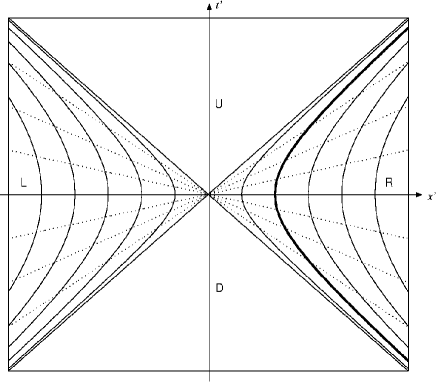
Figure 1: The Rindler coordinate system. Dotted lines are integral lines of $\vec{e}_{\xi}$ and solid lines are integral curves of $\vec{e}_{\tau}$. The thick solid line is the stationary reference curve $C$ or the world line of the uniformly accelerated “observer”.

Viewed from an observer accelerated along the curve $C$ (or any other curve with constant $\xi$) in R, the region L is causally disconnected, since no light signal emitted from $C$ can reach L and no light signal from L can reach $C$. The limiting point (hypersurface) $\xi=0$ between R and L defines an event horizon viewed from $C$. The regions D and U, which are excluded from the Rindler coordinate system are not causally disconnected, but viewed from $C$ the region D lies in the infinite past and U in the infinite future. Thus, D may be viewed as being separated from R by a past horizon and U by a future horizon. This causal structure of the Rindler coordinate system is the underlying reason that a quantum field theory restricted to the right Rindler wedge can be defined.

The boost operator, viewed as the Hamiltonian (7) of the accelerated frame, is different from the original Hamiltonian in one important aspect: It has a spectrum that is not bounded from below. (That is true not only for the special case of linear acceleration, but for the general case of accelerated motion described by the Hamiltonian (1).) The spectrum is in fact symmetric under change of sign as follows from the anti-commutation relation with space inversion,

$$\mbox{$$}PK_{x}=-K_{x}P$$ (9)

As a result a vacuum state defined as the ground state of the Hamiltonian (7) does not exist.

Even without a well-defined ground state the free field Hamiltonian can be written in the conventional form

$$\mbox{$$}H_{O}=\sum\limits_{i}\epsilon_{i}\;a^{{\dagger}}_{i}a_{i}$$ (10)

with $a^{{\dagger}}_{i}$ and $a_{i}$ as creation and annihilation operators, i.e., which satisfy the standard commutation relations

$$\mbox{$$}\left[a_{i},a^{{\dagger}}_{j}\right]=\delta_{ij}\;,\;\;\left[a_{i},a_{j}\right]=\left[a^{{\dagger}}_{i},a^{{\dagger}}_{j}\right]=0$$ (11)

The operators $a^{{\dagger}}_{i}$ can be defined as a linear combination of the usual creation operators associated with free particles in Minkowski space (and $a_{i}$ as the corresponding linear combination of annihilation operators). This follows from the fact that the (free field) expressions for the generators of Lorentz transformations are bilinear in creation and annihilation operators and can be diagonalized without mixing these two types of operators.

With the Hamiltonian written in the form (10) a (generalized) vacuum state can be defined as the state annihilated by the operators $a_{i}$,

$$\mbox{$$}a_{i}\left|0\right\rangle=0$$ (12)

and the full space of states can be generated in the standard way by repeated application of the creation operators on the vacuum state. The operators $a_{i}^{{\dagger}}$ create excitations (particles) with energy $\epsilon_{i}$ with reference to the accelerated coordinate frame, and since $\left|0\right\rangle$ is not the ground state of the Hamiltonian, excitations both with positive and negative energy $\epsilon_{i}$ can be created from the vacuum state $\left|0\right\rangle$. Note that when the operators $a_{i}$ are defined as linear combinations of the standard (Minkowski space) annihilation operators, the generalized vacuum of the accelerated frame is identical to the ordinary Minkowski vacuum.

III.2 The transformed vacuum

In the above description of the field theory vacuum no particles are present in the physical (Minkowski) space. The Unruh effect in this picture is understood as due to processes where the accelerated detector is excited by emitting negative energy particles. However, the symmetry of the spectrum of $H_{O}$ between positive and negative values allows alternative definitions of the vacuum state and the particle excitations. A particular choice gives rise to the Fulling-Rindler vacuum, where all excitations restricted to the right Rindler wedge $R$ have positive energy. In this picture the Minkowski vacuum state contains particles relative to the accelerated vacuum state and the Unruh effect is described as due to absorption of such (positive energy) particles.

To discuss this point we focus on the field operator of the (real) Klein-Gordon field. When expressed in terms of the Rindler coordinates, it can be written as

$$\mbox{$$}\phi(\xi,y,z,\tau)=\sum\limits_{i}(e^{-i\epsilon_{i}\tau}f_{i}(\xi,y,z)a_{i}+e^{i\epsilon_{i}\tau}f_{i}^{*}(\xi,y,z)a^{{\dagger}}_{i}\,)$$ (13)

with $f_{i}(\xi,y,z)\;a_{i}$ and $f_{i}^{*}(\xi,y,z)$ as stationary solutions (with respect to $\tau$) of the Klein-Gordon equation,

$$\mbox{$$}\big{(}\frac{1}{\xi}\,\partial_{\xi}\,\xi\,\partial_{\xi}+\partial_{y}^{2}+\partial_{z}^{2}+(\epsilon_{i}^{2}-m^{2})\big{)}f_{i}(\xi,y,z)=0$$ (14)

To simplify the notation we have labelled the solutions $f_{i}$ with a single (discrete) index $i$, which in reality should be replaced by a set of (continuous) momentum-energy variables that specify the solution. The solutions can be separated into those with positive norm and those with negative norm with respect to the scalar product of the (classical) Klein-Gordon field, which in Rindler coordinates has the form

$$\mbox{$$}\langle f,h\rangle=i\int\frac{1}{a\xi}\left(f^{*}(\xi,y,z)\;\partial_{\tau}h(\xi,y,z)-\partial_{\tau}f^{*}(\xi,y,z)\;h(\xi,y,z)\right)\mathrm{d}\xi\mathrm{d}y\mathrm{d}z$$ (15)

Consistency between the requirement of standard commutation relations for $a_{i}$ and $a_{j}^{{\dagger}}$ and canonical commutation rules for $\phi$ and its conjugate momentum implies that in the expansion (13) the functions $f_{i}$ are positive norm solutions and correspondingly $f_{i}^{*}$ are negative norm solutions. Note that positive norm no longer corresponds to positive frequency, as is the case for Minkowski space quantization.

In the sum included in Eq. (13) the energies $\epsilon_{i}$ take both positive and negative values. Due to the symmetry of the the spectrum it can, however, be rewritten as a sum only over positive energies in the following way,

$$\mbox{$$}\phi(\xi,y,z,\tau) = \sum\limits_{i\,(\epsilon_{i}>0)}[(e^{-i\epsilon_{i}\tau}f_{i}(\xi,y,z)a_{i}+e^{+i\epsilon_{i}\tau}g_{i}(\xi,y,z)b_{i})$$ (16)

$$\hskip 28.45274pt+(e^{i\epsilon_{i}\tau}f_{i}^{*}(\xi,y,z)a^{{\dagger}}_{i}+e^{-i\epsilon_{i}\tau}g_{i}^{*}(\xi,y,z)b^{{\dagger}}_{i}\,)]$$

$$= \sum\limits_{i\,(\epsilon_{i}>0)}[e^{-i\epsilon_{i}\tau}(f_{i}(\xi,y,z)a_{i}+g_{i}^{*}(\xi,y,z)b^{{\dagger}}_{i})$$

$$\hskip 28.45274pt+e^{i\epsilon_{i}\tau}(f_{i}^{*}(\xi,y,z)a^{{\dagger}}_{i}+g_{i}(\xi,y,z)b_{i}\,)]$$

In this expression we have explicitly separated out the negative energy solutions, which we refer to as $g_{i}$, and introduced the notation $b_{i}$ and $b_{i}^{{\dagger}}$ for the corresponding annihilation and creation operators.

Since the operators $a_{i}$ and $b_{i}^{{\dagger}}$ have the same time-dependent prefactor, a Bogoliubov transformation may be performed,

$$\mbox{$$}a_{i} = \tilde{a}_{i}\cosh\chi_{i}+\tilde{b}_{i}^{{\dagger}}\sinh\chi_{i}$$

$$b_{i}^{{\dagger}} = \tilde{a}_{i}\sinh\chi_{i}+\tilde{b}_{i}^{{\dagger}}\cosh\chi_{i}$$ (17)

The transformed operators $\tilde{a}_{i}$ and $\tilde{b}_{i}^{{\dagger}}$ and their hermitian conjugates satisfy the same commutation relations as the original creation and annihilation operators and the field operator expressed in terms of the new ones has the same form as before,

$$\mbox{$$}\phi(\xi,y,z,\tau) = \sum\limits_{i\,(\epsilon_{i}>0)}[e^{-i\epsilon_{i}\tau}(\tilde{f}_{i}(\xi,y,z)\tilde{a}_{i}+\tilde{g}_{i}^{*}(\xi,y,z)\tilde{b}^{{\dagger}}_{i})$$ (18)

$$\hskip 28.45274pt+e^{i\epsilon_{i}\tau}(\tilde{f}_{i}^{*}(\xi,y,z)\tilde{a}^{{\dagger}}_{i}+\tilde{g}_{i}(\xi,y,z)\tilde{b}_{i}\,)]$$

with transformed fields

$$\mbox{$$}\tilde{f}_{i}(\xi,y,z) = f_{i}(\xi,y,z)\cosh\chi_{i}+g_{i}^{*}(\xi,y,z)\sinh\chi_{i}$$

$$\tilde{g}_{i}(\xi,y,z) = f_{i}^{*}(\xi,y,z)\sinh\chi_{i}+g_{i}(\xi,y,z)\cosh\chi_{i}$$ (19)

A new generalized vacuum state may be defined relative to the transformed operators,

$$\mbox{$$}\tilde{a}_{i}\left|\tilde{0}\right\rangle=0\,,\,\;\tilde{b}_{i}\left|\tilde{0}\right\rangle=0$$ (20)

and this is different from the Minkowski vacuum due to the mixing of creation and annihilation operators. In fact a continuum of different vacuum states can be defined in this way, but like the Minkowski vacuum they generally suffer from the defect that both positive and negative energy excitations (of the accelerated Hamiltonian) may be created from the state $\left|\tilde{0}\right\rangle$. The Minkowski vacuum will now contain field quanta relative to the transformed vacuum and for a detector that is stationary in the accelerated frame there will therefore be two sources for excitations. The detector can either be excited by absorbing positive energy quanta or by emitting negative energy quanta.

A particular transformation can be chosen where all negative energy field quanta are located beyond the event horizon, i.e., in the left Rindler wedge $L$ ($\xi<0$). This gives rise to the Rindler or Fulling vacuum, which is a true vacuum state in the sense that it is the ground state of $H_{O}$, provided all states are restricted to the right Rindler wedge $R$. This possibility can be viewed as due to the symmetry of the theory under $PCT$, which gives rise to a relation between the functions $f_{i}$ and $g_{i}$ on the two sides of the horizon Sewell82 ; Hughes85 ; Bell85 . We will give a simple demonstration of this.

The $PCT$ transformation $\theta$ acts on the field operator in the following way,

$$\mbox{$$}\theta\phi\,(\xi,y,z,\tau)\,\theta^{-1}=\phi^{{\dagger}}(-\xi,-y,-z,\tau)$$ (21)

Like the parity operator, $\theta$ anticommutes with the boost operator and therefore maps positive energy solutions into negative energy solutions,

$$\mbox{$$}\theta a_{i}\,\theta^{-1}=b_{i}\;,\;\;\theta b_{i}\,\theta^{-1}=a_{i}$$ (22)

Since $\theta$ acts as an antilinear operator this gives the following relation between the functions $f_{i}$ and $g_{i}$,

$$\mbox{$$}g_{i}(\xi,y,z)=f_{i}^{*}(-\xi,-y,-z)$$ (23)

We further note that the definition of the Rindler coordinates implies that the strong space-time reflection $PT$ can be performed either by an inversion $\xi\rightarrow-\xi$ (together with $y\rightarrow-y,z\rightarrow-z$) or by an analytic continuation $\tau\rightarrow\tau\pm\pi i/a$. This is related to the fact that $PT$ can be viewed as a complex extension of the Lorentz transformations (which here induce translations in $\tau$) Bell55 . As a result $f_{i}(-\xi,-y,-z)$ can be related to $f_{i}(\xi,y,z)$ by an analytic continuation of the full time-dependent solution of the Klein-Gordon equation.

Since the operators $a_{i}$ and $b_{i}$ have been introduced without mixing the original Minkowski space annihilation operators with creation operators, this means that the corresponding functions $f_{i}$ and $g_{i}$ include only positive frequency components with respect to Minkowski time. We can therefore expand $f_{i}$ as follows,

$$\mbox{$$}e^{-i\epsilon_{i}\tau}f_{i}(\xi,y,z) = \int d^{3}pF_{i}(\vec{p})e^{-i(\omega_{p}t-\vec{p}\cdot\vec{x})}\;,\;\;\;\omega_{p}=\sqrt{p^{2}+m^{2}}$$ (24)

$$= \int d^{3}pF_{i}(\vec{p})e^{i(p_{y}y+p_{z}z)}e^{-i\xi(\omega_{p}\sinh a\tau-p_{x}\cosh a\tau)}$$

A similar expression is valid for $g_{i}$. For a complex extension $\tau\rightarrow\tau+i\vartheta/a$, the change of the exponential, factor is

$$\mbox{$$}e^{-i\xi(\omega_{p}\sinh a\tau-p_{x}\cosh a\tau)}\rightarrow e^{-i\xi\cos\vartheta(\omega_{p}\sinh a\tau-p_{x}\cosh a\tau)}e^{\xi\sin\vartheta(\omega_{p}\cosh a\tau-p_{x}\sinh a\tau)}$$ (25)

where the last factor determines whether the integral (24) is convergent or divergent for large $p$. Since $\omega_{p}>p$, convergence implies that for positive $\xi$ the Rindler time $\tau$ should be analytically continued in the lower complex half plane, while for negative $\xi$ it should be continued in the upper half plane. With this prescription for the analytic continuation of the solutions to the space-time inverted point we find

$$\mbox{$$}f_{i}(-\xi,-y,-z) = e^{-\frac{\epsilon_{i}\pi}{a}}f_{i}(\xi,y,z)\;,\;\;\xi>0$$

$$g_{i}(-\xi,-y,-z) = e^{\frac{\epsilon_{i}\pi}{a}}\;g_{i}(\xi,y,z)\;,\quad\xi>0$$ (26)

which, together with (23), finally leads to the following relations between $f_{i}$ and $g_{i}$ in the same Rindler wedge

$$\mbox{$$}f_{i}(\xi,y,z)=e^{+\frac{\epsilon_{i}\pi}{a}}\;g_{i}^{*}(\xi,y,z)\;,\quad\xi>0$$

$$f_{i}(\xi,y,z)=e^{-\frac{\epsilon_{i}\pi}{a}}\;g_{i}^{*}(\xi,y,z)\;,\quad\xi<0$$ (27)

Thus, if we define transformed fields as

$$\mbox{$$}\tilde{f}_{i}(\xi,y,z) = \sinh(\frac{\epsilon_{i}\,\pi}{2a})^{-\frac{1}{2}}[e^{+\frac{\epsilon_{i}\pi}{2a}}f_{i}(\xi,y,z)-e^{-\frac{\epsilon_{i}\pi}{2a}}\;g_{i}^{*}(\xi,y,z)]$$

$$\tilde{g}_{i}(\xi,y,z) = \sinh(\frac{\epsilon_{i}\,\pi}{2a})^{-\frac{1}{2}}[e^{+\frac{\epsilon_{i}\pi}{2a}}g_{i}(\xi,y,z)-e^{-\frac{\epsilon_{i}\pi}{2a}}\;f_{i}^{*}(\xi,y,z)]$$ (28)

which corresponds to a transformation of the form (III.2) with

$$\mbox{$$}\cosh\chi_{i}=\frac{e^{+\frac{\epsilon_{i}\pi}{2a}}}{\sqrt{2\sinh(\frac{\epsilon_{i}\,\pi}{a})}}\;,\;\;\sinh\chi_{i}=-\frac{e^{-\frac{\epsilon_{i}\pi}{2a}}}{\sqrt{2\sinh(\frac{\epsilon_{i}\,\pi}{a})}}$$ (29)

then the transformed field $\tilde{f}_{i}$ vanishes identically for $\xi<0$ and $\tilde{g}_{i}$ vanishes identically for $\xi>0$. Thus, for this value for the transformation parameter $\chi_{i}$ the field modes of the two sides of the horizon are completely decoupled.

In terms of the new creation and annihilation operators Minkowski vacuum contains (particle) excitations,

$$\mbox{$$}\left\langle\tilde{a}_{i}^{{\dagger}}\tilde{a}_{i}\right\rangle_{M} = \sinh^{2}\chi_{i}\left\langle b_{i}b_{i}^{{\dagger}}\right\rangle_{M}$$ (30)

$$= \frac{e^{-\frac{\epsilon_{i}\pi}{a}}}{2\sinh(\frac{\epsilon_{i}\,\pi}{a})}$$

$$= \frac{1}{e^{\frac{2\pi\epsilon_{i}}{a}}-1}$$

The expression corresponds to a thermal Bose-Einstein distribution over the excited levels, with temperature given by

$$\mbox{$$}k_{B}T_{a}=\frac{a}{2\pi}$$ (31)

which is the Unruh temperature.

IV Planar motion with acceleration and rotation

We now consider motion along stationary worldlines where the acceleration is no longer linear. In these cases the co-moving, Fermi-Walker transported frame will be rotating relative to an inertial rest frame. Thus, $\boldsymbol{\omega}\neq 0$, and the general Hamiltonian is given by (2). We restrict, in this section, the motion to be planar, with the Hamiltonian given by

$$\mbox{$$}{H}_{O}\,=\,{H}-a{K}_{x}-\omega{J}_{z}$$ (32)

It is convenient to simplify the Hamiltonian by making a boost in the $y$-direction in addition to a shift of origin in the $x$-direction. With $\beta$ as the velocity parameter the transformation from the lab frame to the boosted coordinates is

$$\mbox{$$}y^{\prime}=\gamma(y-\beta t)\;,\;\;\;x^{\prime}=x+\frac{a}{a^{2}-\omega^{2}}\;,\;\;\;z^{\prime}=z\;,\;\;\;t^{\prime}=\gamma(t-\beta y)$$ (33)

and the Hamiltonian expressed in terms of operators of the transformed frame is

$$\mbox{$$}{H}_{O}=\gamma\left[\,-\frac{\omega(\omega-a\beta)}{a^{2}-\omega^{2}}{H}^{\prime}+\frac{\omega(a-\omega\beta)}{a^{2}-\omega^{2}}{P}_{y^{\prime}}-\left(a-\beta\omega\right){K}_{x^{\prime}}-\left(\omega-\beta a\right){J}_{z^{\prime}}\,\right]$$ (34)

with $P_{y^{\prime}}$ as the translation operator in the $y^{\prime}$-direction.

We note that when $a>\omega$ the velocity parameter can be chosen as $\beta=\omega/a$ so that the coefficients of $H_{O}$ and $J_{z}$ vanish. The Hamiltonian then simplifies to

$$\mbox{$$}{H}_{O}=-\sqrt{a^{2}-\omega^{2}}\,{K}_{x^{\prime}}+\frac{\omega}{\sqrt{a^{2}-\omega^{2}}}\,{P}_{y^{\prime}}\;,\;\;\;\;a>\omega$$ (35)

If instead $a<\omega$ it can be chosen as $\beta=a/\omega$ so that the coefficients of $K_{x^{\prime}}$ and $P_{y^{\prime}}$ vanish. The form of the Hamiltonian then is

$$\mbox{$$}{H}_{O}=\frac{\omega}{\sqrt{\omega^{2}-a^{2}}}\,{H}^{\prime}-\sqrt{\omega^{2}-a^{2}}\,{J}_{z^{\prime}}\;,\;\;\;\;a>\omega$$ (36)

We shall discuss these two cases separately. For simplicity we suppress in this section the $z$-coordinate, since the motion is restricted to the $(x,y)$-plane.

IV.1 Accelerated coordinates for planar trajectories with rotation

The case $a>\omega$  

The stationary curves generated by the time evolution operator (35) are described by the (tangent) vector field

$$\mbox{$$}\vec{e}_{\tau}=\sqrt{a^{2}-\omega^{2}}\left(x^{\prime}\vec{e}_{t^{\prime}}+t^{\prime}\vec{e}_{x^{\prime}}\right)-\frac{\omega}{\sqrt{a^{2}-\omega^{2}}}\vec{e}_{y^{\prime}}$$ (37)

which is here expressed in terms of the coordinates of the boosted inertial frame. The expression shows that the trajectory projected on the $(t^{\prime},x^{\prime})$-plane is the same as for hyperbolic motion, i.e., for linear motion with constant proper acceleration. In addition there is motion in the $y^{\prime}$ direction, and measured with the time coordinate $\tau$ of the accelerated frame, this component of the motion corresponds to a drift with constant velocity. However, measured with the inertial time $t^{\prime}$ the velocity in the $y^{\prime}$-direction will slow down with increasing $|t^{\prime}|$ due to time dilatation. This means that asymptotically (for $t^{\prime}\rightarrow\pm\infty$) the motion will be dominated by the $x^{\prime}$-component.

It is interesting to note that there is no rotation involved in the motion as seen from the boosted inertial frame. The rotation of the curve, as measured in the local inertial rest frame, can be seen as due to composition of boosts in two different directions, in the $x^{\prime}$-direction and the $y^{\prime}$-direction, when transforming to the rest frame of the stationary curve.

The decomposition of the motion in the $x^{\prime}$ and $y^{\prime}$ directions motivates the introduction of a new set of Rindler coordinates which are adjusted to the component with linear acceleration in the $x^{\prime}$ direction,

$$\mbox{$$}t^{\prime} =\xi^{\prime}\sinh\sqrt{a^{2}-\omega^{2}}\tau^{\prime}\;,\;\;x^{\prime}=\xi^{\prime}\cosh\sqrt{a^{2}-\omega^{2}}\tau^{\prime}$$ (38)

In terms of these Rindler coordinates the vector field (37) takes the form

$$\mbox{$$}\vec{e}_{\tau}=\sqrt{a^{2}-\omega^{2}}\vec{e}_{\tau^{\prime}}-\frac{\omega}{\sqrt{a^{2}-\omega^{2}}}\vec{e}_{y^{\prime}}$$ (39)

Since we now in reality are working with four different coordinate systems, we make the following reminder: The original inertial frame with coordinates $(t,x,y)$ coincides with the inertial rest frame of the accelerated world line at time $t=0$. If we denote by $(\tau,\xi,\eta)$ the accelerated coordinates, we may therefore identify $\xi$ with $x$ and $\eta$ with $y$ at $t=\tau=0$. The boosted inertial frame, with coordinates $(t^{\prime},x^{\prime},y^{\prime})$ moves with constant velocity along the $y$-axis. This frame is useful since it decomposes the motion in two independent components in the $x^{\prime}$- and $y^{\prime}$-directions. Finally the Rindler coordinate system, with coordinates $(\tau^{\prime},\xi^{\prime},y^{\prime})$ is the rest frame of the $x$-component of the motion. It is not identical to the accelerated frame of the stationary orbit, since it does not take into account the motion in the y-direction. We note that the $z$ coordinate is common for all coordinate systems since all motion takes part in the $x,y$ directions only.

The reference orbit $C$ is defined as the stationary curve where the coordinate time $\tau$ coincides with the proper time, i.e., $\vec{e}_{\tau}\cdot\vec{e}_{\tau}=-1$. From the expression (38), we find the Rindler coordinates of this orbit to be, when expressed with the proper time $\tau$ as curve parameter

$$\tau^{\prime}(\tau) =\,\tau$$

$$\xi^{\prime}(\tau) =\frac{a}{a^{2}-\omega^{2}}$$

$$y^{\prime}(\tau) =-\frac{\omega}{\sqrt{a^{2}-\omega^{2}}}\,\tau$$

$$z(\tau) =0$$ (40)

The $\xi^{\prime}$ coordinate is constant, but there is a constant drift in the $y^{\prime}$ direction.

The causal structure of space time as seen from the accelerated orbit is most easily discussed in the boosted inertial frame. Since the asymptotic behaviour of the stationary curve is dominated by the $x$-component of the motion, there are event horizons located in the same positions as for linear accelerated motion. There is a past horizon at $x^{\prime}=-ct^{\prime}$, so that no light signal emitted from the accelerated orbit can reach points with $x^{\prime}<-ct^{\prime}$, and there is a future horizon at $x^{\prime}=ct^{\prime}$ so that no light signal emitted from a point $x^{\prime}<-ct^{\prime}$ can reach the accelerated orbit. The location of these horizons in the rest frame of the accelerated orbit can be found by use of the identification of space coordinates of this frame with those of the (original) inertial frame at $t=0$. The Lorentz transformation (33) gives the locations at

$$\mbox{$$}\eta=\pm\frac{\sqrt{a^{2}-\omega^{2}}}{\omega}(\xi+\frac{a}{a^{2}-\omega^{2}})$$ (41)

where “+” gives the past horizon and “-” gives the future horizon. Note that this expression is valid not only for $\tau=0$, but for all $\tau$, since the situation in the accelerated frame is stationary. In the same way as for the horizon of a linearly accelerated orbit the horizons here correspond to singularities of the accelerated coordinate system, where the time coordinate is ill-defined.

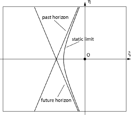
Figure 2: Event horizons and static limit in the accelerated frame. The stationary reference curve $C$ corresponds to the origin $O$. The two directions in the plane correspond to the two space-like directions where $\xi$ coincides with $x$ of the fixed inertial frame and $\eta$ coincides with $y$ for $t=0$. The distances to the horizon and to the static limit are determined by the two parameters $a$ and $\omega$.

Since the accelerated frame is rotating, there exists a static limit in this coordinate system. This is the limit for where physical objects can be stationary with respect to the coordinate system. Beyond the static limit the stationary curves become space-like rather than time-like. The location of the static limit can be found by considering the norm of the coordinate vector $\vec{e}_{\tau}$ as a function of the coordinates,

$$\mbox{$$}\vec{e}_{\tau}\cdot\vec{e}_{\tau}=\vec{e}_{\tau^{\prime}}\cdot\vec{e}_{\tau^{\prime}}+\frac{\omega^{2}}{a^{2}-\omega^{2}}\,\vec{e}_{y^{\prime}}\cdot\vec{e}_{y^{\prime}}=\left(a^{2}-\omega^{2}\right)({x^{\prime}}^{2}-{t^{\prime}}^{2})-\frac{\omega^{2}}{a^{2}-\omega^{2}}$$ (42)

The norm changes from negative to positive at the static limit. In order to find its location in terms of the coordinates of the accelerated frame, we again make use of the fact that the coordinates $(\xi,\eta)$ coincide with $(x,y)$ for $t=0$ (or equivalently for $\tau=0$). By use of the Lorentz transformation (33) we find for $t=0$ (and with $(x,y)$ replaced by $(\xi,\eta)$),

$$\mbox{$$}\vec{e}_{\tau}\cdot\vec{e}_{\tau}=\left(a^{2}-\omega^{2}\right)\Big{[}(\xi+\frac{a}{a^{2}-\omega^{2}})^{2}-\eta^{2}\frac{\omega^{2}}{a^{2}-\omega^{2}}\Big{]}-\frac{\omega^{2}}{a^{2}-\omega^{2}}$$ (43)

The scalar product vanishes for

$$\mbox{$$}\left(\frac{a^{2}-\omega^{2}}{\omega}\right)^{2}(\xi+\frac{a}{a^{2}-\omega^{2}})^{2}-(a^{2}-\omega^{2})\eta^{2}=1$$ (44)

This defines a hyperbola in the $(\xi,\eta)$-plane, with the event horizons as asymptotes. Viewed from the stationary orbit $C$, which is given by $(\xi,\eta)=(0,0)$, the event horizons are located behind the static limit.

We note that when $\omega\rightarrow 0$, where the case of the linear acceleration is recovered, both the event horizons tend to the same straight line $\xi\rightarrow-1/a$ and the static limit merges with the horizons.

When the rotation instead increases and $\omega\rightarrow a$, the distance to both horizons go to infinity and they therefore disappear from the $(\xi,\eta)$-plane. The static limit on the other hand stays at a finite distance and changes to a parabola.

The case $a<\omega$

In this case the (accelerated) time translation operator is given by (36) and the corresponding vector field is

$$\mbox{$$}\vec{e}_{\tau}=\frac{\omega}{\sqrt{\omega^{2}-a^{2}}}\,\vec{e}_{t^{\prime}}+\sqrt{\omega^{2}-a^{2}}\,(x^{\prime}\vec{e}_{y^{\prime}}-y^{\prime}\vec{e}_{x^{\prime}})$$ (45)

This describes circular motion, as can be seen explicitly by changing to cylindrical coordinates

$$\mbox{$$}x^{\prime}=r\cos\theta\;\;\;y^{\prime}=r\sin\theta$$ (46)

which gives

$$\vec{e}_{\tau}\,=\,\frac{\omega}{\sqrt{\omega^{2}-a^{2}}}\vec{e}_{t^{\prime}}+\sqrt{\omega^{2}-a^{2}}\;\vec{e}_{\theta}$$ (47)

At $\tau=0$, the reference curve $C$ is located at $x^{\prime}=-a/(\omega^{2}-a^{2})$, corresponding to $r=a/(\omega^{2}-a^{2})$ and $\theta=\pi$. Expressed as a function of the proper time coordinate $\tau$, the trajectory is

$$t^{\prime} =\frac{\omega}{\sqrt{\omega^{2}-a^{2}}}\,\tau$$

$$r =\frac{a}{\omega^{2}-a^{2}}$$

$$\theta =\pi+\sqrt{\omega^{2}-a^{2}}\,\tau$$ (48)

This space-time curve describes motion in a circle of radius $r=a/(\omega^{2}-a^{2})$ with angular velocity $\Omega=(\omega^{2}-a^{2})/\omega$ relative to the boosted inertial frame.

In this case there clearly is no event horizon since the orbit is restricted to a bounded region of space, so that a signal from an event anywhere in space will be able to reach the space-time curve and any space-time point can be reached by a light signal from a point on the curve. However, also for circular motion there is a static limit defined by the accelerated coordinate system. The norm of the vector $\vec{e}_{\tau}$ now is

$$\vec{e}_{\tau}\cdot\vec{e}_{\tau}\,=\,\frac{\omega^{2}}{\omega^{2}-a^{2}}-r^{2}\left(\omega^{2}-a^{2}\right)$$ (49)

hence, $\vec{e}_{\tau}$ becomes spacelike for $r>\omega/(\omega^{2}-a^{2})$, which is the radius where the velocity of the rotating coordinate system exceeds the velocity of light. The location of this static limit in the accelerated coordinates can be found in the same way as before, that is by performing a boost to the inertial frame that coincides with the rotating frame at $t=0$ and by making the identification $(x,y)\rightarrow(\xi,\eta)$ for $t=0$. The location is determined by ,

$$\mbox{$$}\left(\frac{\omega^{2}-a^{2}}{\omega}\right)^{2}\left(\xi-\frac{a}{\omega^{2}-a^{2}}\right)^{2}+\left(\omega^{2}-a^{2}\right)\eta^{2}\,=\,1$$ (50)

which is the equation for an ellipse, with the major semiaxis in the $\xi$-direction and the minor semiaxis in the $\eta$-direction. We can interpret this shape of the static limit, as a deformation of a circle of radius $\omega/(\omega^{2}-a^{2})$ in the $(x^{\prime},y^{\prime})$-plane. The deformation is due to the length contraction in the $y^{\prime}$ (or $\eta$)-direction introduced by the transformation to the rest frame of the accelerated trajectory.

From the above discussion it follows that there is a qualitative difference between the cases $a>\omega$ and $a<\omega$. In the first case the (3-)space projection of the accelerated trajectory is unbounded in any inertial frame, and the asymptotic behavior implies that event horizons exist. In the latter case, the motion is bounded and can be viewed as circular motion in a properly chosen inertial frame. No event horizons exist in this case. The limiting case $a=\omega$ can be reached from both sides. Viewed as a limiting case of circular motion it corresponds to the ultra-relativistic limit where the velocity of circulation tends to the velocity of light.

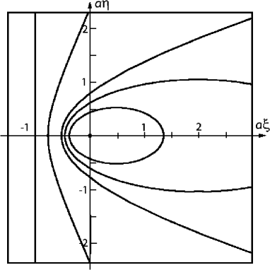
Figure 3: The static limit for different values of $\omega/a$ as seen in the accelerated coordinate frame. There is a continuous change from $\omega<a$ to $\omega>a$. From left to right the curves in the $(\xi,\eta)$-plane correspond to $\omega=0$ (straight line), $\omega=0.3a$ (hyperbola), $\omega=a$ (parabola), $\omega=1.2a$ and $\omega=1.4a$ (both ellipses). The coordinates are measured in units of $1/a$.

One should note, however, that this qualitative difference has mainly to do with the asymptotic form of the space time curves as viewed from an inertial frame. For a finite time interval, or viewed in the co-moving frame, there is no singular behaviour at the point $a=\omega$. This is demonstrated in Fig.3 where the static limit as viewed in the accelerated coordinate system, is shown for several different values of $\omega/a$. The static limit changes continuously from a hyperbola (with the event horizons as asymptotes) for $a>\omega$ through a parabola for $a=\omega$ to an ellipse for $a<\omega$.

IV.2 Vacuum states in the accelerated frame

We first consider the case $a>\omega$ with the Hamiltonian given by (35). We note that since ${K}_{x^{\prime}}$ and ${P}_{y^{\prime}}$ commute, the eigenstates of the Hamiltonian $H_{O}$ can also be chosen as eigenstates of the boost operator ${K}_{x^{\prime}}$ and the translation operator $P_{y^{\prime}}$ . This means that the Hamiltonian can be diagonalized in the same way as for linear acceleration. Thus, also for $\omega\neq 0$ and $a>\omega$ there exists a continuum of possible vacuum states that are connected by Bogoliubov transformations which mix creation and annihilation operators. We focus again on the particular transformation that separate the field modes on the two sides of the horizons. The field modes $\tilde{f}_{i}$ corresponding to negative eigenvalues of $K_{x^{\prime}}$ are the relevant ones for the reference curve $C$ in the right Rindler wedge, since these are the ones that have positive norm on that wedge. We denote these eigenvalues by $-\Omega$, with $\Omega>0$.

The field modes $\tilde{f}_{i}$ can be identified with the corresponding modes previously discussed, except that they are now functions of the new Rindler coordinates $(\tau^{\prime},\xi^{\prime},y^{\prime},z)$. The explicit form is

$$\tilde{f}_{k_{y^{\prime}}k_{z}\Omega}(\tau^{\prime},\xi^{\prime},y^{\prime},z)=\begin{cases}\frac{\sqrt{\sinh(\pi\Omega)}}{2\pi^{2}}e^{-i\Omega\sqrt{a^{2}-\omega^{2}}\tau^{\prime}}e^{i(k_{y^{\prime}}y^{\prime}+k_{z}z)}K_{i\Omega}(\Xi\xi^{\prime}),&\xi^{\prime}>0,\;\Omega>0\\ 0,&\xi^{\prime}<0,\;\Omega>0\end{cases}$$ (51)

where the index $i$ here is specified as the set of eigenvalues $\Omega$, $k_{y^{\prime}}$ and $k_{z}$ of the operators ${K}_{x^{\prime}}$, ${P}_{y^{\prime}}$ and ${P}_{z}$, and the parameter $\Xi$ is

$$\mbox{$$}\Xi=\sqrt{k_{y}^{2}+k_{z}^{2}+m^{2}}$$ (52)

with $m$ as the mass of the Klein-Gordon particles. The function $K_{i\Omega}$, which is a solution of the Klein-Gordon equation in Rindler coordinates (14), is a modified Bessel function (a MacDonald function of imaginary order) MacDonald .

Even if the wave functions are the same as for linear acceleration one should note an important difference. For linear acceleration the restriction of the wave functions to the accessible side of the event horizon will at the same time be a restriction of the energies to positive values. Here this restriction means that $\Omega>0$ for the relevant eigenvalue of the boost operator. However, this eigenvalue is no longer proportional to the energy eigenvalue, since the energy also gets contribution from ${P}_{y^{\prime}}$. The eigenvalues of $H_{O}$ are

$$\mbox{$$}\epsilon=\sqrt{a^{2}-\omega^{2}}\;\Omega+\frac{\omega}{\sqrt{a^{2}-\omega^{2}}}k_{y^{\prime}}$$ (53)

For sufficiently large negative $k_{y^{\prime}}$ the last term will dominate the first term and give a negative energy eigenvalue.

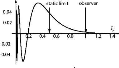
Figure 4: Stationary solution of the Klein-Gordon equation in the Rindler coordinates. The figure shows a solution with energy $\epsilon=0$ for the Hamiltonian of the accelerated coordinate system. For all negative values $\epsilon<0$ the solutions have only an exponential tail on the ”physical” side of the static limit.

It is of interest to note that these negative energy solutions will essentially be located between the event horizon and the static limit. To see this we first note that the static limit of the accelerated coordinate system, as well as the horizons and the reference curve $C$ have fixed $\xi^{\prime}$ coordinates, even if the Rindler coordinate system does not define a rest frame for the accelerated observer. Thus both horizons have Rindler coordinate $\xi_{ho}=0$, the static limit is located at $\xi_{sl}=\omega/(a^{2}-\omega^{2})$ and the accelerated observer is located at $\xi^{\prime}=a/(a^{2}-\omega^{2})$. We next note that the energy eigensolutions (51) have an oscillatory behaviour for small $\xi^{\prime}$ but are exponentially damped for large $\xi^{\prime}$. As shown by the Klein Gordon equation the transition point between the two types of behaviour is $\xi^{\prime}_{tr}=\Omega/\Xi$. For negative energy states we have $\Omega<|k_{y^{\prime}}|\omega/(a^{2}-\omega^{2})$, as follows from (53), which implies the inequality

$$\mbox{$$}\xi^{\prime}_{ho}<\xi^{\prime}_{tr}<\xi^{\prime}_{sl}$$ (54)

Thus, the negative energy solutions are are mainly located inside the static limit, but this is not fully so due to the exponential tail of the wave functions, as illustrated in Fig.4. The penetration of the negative energy states into the physical region of the accelerated frame is important for excitations of an accelerated detector. The modes can contribute to the excitations since negative energy quanta can be emitted into the modes by the detector.

To summarize, for accelerated orbits which involve rotation in addition to acceleration, event horizons exist as long as $a>\omega$. In the same way as discussed for linear acceleration the field modes can be defined so that they are restricted to one side of the horizons. This will involve a Bogoliubov transformation of the Minkowski space creation and annihilation operators. The transformed vacuum state is then the Fulling-Rindler vacuum associated with uniform acceleration of the $x^{\prime}$ component of the space time trajectory. However, the Fulling vacuum is not a true vacuum state since there now are negative energy states present in the right Rindler wedge. Thus, the negative energy states are no longer restricted to the space-time region behind the horizons, as it is for linear acceleration. On the other hand these states are mainly located behind the static limit, but this region is not causally disconnected from the reference curve $C$. The presence of negative energy states implies that the Hamiltonian does not have a well defined ground state even after separating the modes behind the horizons from those in front of the horizons.

Even if the Fulling vacuum is no longer a true vacuum it is convenient to refer to this state and the corresponding excitations in the description of the (generalized) Unruh effect, since the modes that are causally disconnected are explicitly removed from the description. As already discussed there are now two sources for excitation of an accelerated detector. The detector can be excited by absorbing positive energy excitations (which are present when the Minkowski vacuum state is expressed in terms of Rindler space excitations) and it can be excited by emitting negative energy excitations. This situation is quite analogous to the situation of a stationary detector close to the static limit of a rotating black hole. In that case the latter process, emission of negative energy excitations has a classical analogy in the Penrose effect Penrose69 , where a physical system can gain energy by placing an object into one of the negative energy orbits between the static limit and the horizon.

We now turn to the case $\omega>a$, which we will discuss more briefly. The Hamiltonian of the accelerated frame gets the simple form (36), which is composed by the Minkowski space Hamiltonian $H$ and the rotation generator $J_{z}$. Since these two operators commute, due to rotational invariance, the eigenstates of the accelerated Hamiltonian $H_{O}$ are the same as those of the Minkowski space Hamiltonian, when these are expressed as angular momentum states. The energy eigenvalues have the form

$$\mbox{$$}\epsilon=\frac{\omega}{\sqrt{\omega^{2}-a^{2}}}\;E-\sqrt{\omega^{2}-a^{2}}\;m_{z}$$ (55)

where $E$ is the eigenvalue of $H$ and $m_{z}$ the eigenvalue of $J_{z}$.

In this case there are negative energy solutions when $m_{z}$ is sufficiently large compared to $E$. This means that Minkowski space is no longer the ground state of the Hamiltonian and there is no other true vacuum state. For $a<\omega$ there is no event horizon, as we have already discussed, but there is a static limit, and again one can show that the negative energy solutions have an oscillatory behaviour outside the static limit, but are exponentially damped inside. Related to the disappearance of the event horizons there is a lack of symmetry between positive and negative eigenvalues in the spectrum of $H_{O}$ (55). Thus, there is no longer a freedom of mixing creation and annihilation operators when the Hamiltonian is diagonalized. In this sense we are stuck with the standard creation and annihilation operators. This means that Minkowski space contains no excitations (relative to these operators) and the excitation of a detector that is accelerated in a circular orbit is therefore (as described in the accelerated frame) only due to the emission of negative energy quanta.

We will however again stress that the qualitatively different descriptions of the cases $a>\omega$ and $a<\omega$ is due to the difference of asymptotic behaviour of the accelerated orbits. In reality the excitation (and de-excitation) of an accelerated detector reaches equilibrium in a finite time determined by $a$ and $\omega$, and the asymptotic form of the curves is therefore less important. This means that the excitation spectrum changes continuously when $\omega$ is changed through the value $\omega=a$, and we will show this explicitly in the next section.

V Particle detectors and thermodynamics

For linear acceleration the Minkowski vacuum state has the form of a thermally excited state of temperature $T_{a}=a/(2\pi k_{B})$, when the state is expressed in terms of the Fulling field quanta. This representation of the Minkowski vacuum, as a hot state, has relevance also for (planar) accelerated motion with rotation, when $a>\omega$ and therefore event horizons exist.

To examine the interpretation of the Minkowski vacuum in the accelerated frame when $\omega\neq 0$, we return to the Bogoliubov transformation (III.2) that relates the Minkowski and Fulling field quanta. The corresponding transformation between the vacuum states is

$$\mbox{$$}\left|0_{M}\right\rangle={\cal K}e^{-\sum\limits_{i}\tanh\chi_{i}\,\tilde{a}_{i}^{{\dagger}}\tilde{b}_{i}^{{\dagger}}}\left|0_{F}\right\rangle\;,\;\;{\cal K}=e^{-\sum\limits_{i}\ln(\cosh\xi_{i})}$$ (56)

where ${\cal K}$ is a normalization factor and $\left|0_{M}\right\rangle$ is the Minkowski vacuum state. $\left|0_{F}\right\rangle$ is the Fulling vacuum state, which is the state annihilated by the operators $\tilde{a}_{i}$ of the right Rindler wedge as well as the operators $\tilde{b}_{i}$ of the left Rindler wedge. The corresponding field modes we again label by the index $i$. With the parameter $\chi_{i}$ specified by (29) the Minkowski vacuum state can be written as

$$\mbox{$$}\left|0_{M}\right\rangle = {\cal K}e^{-\sum\limits_{i}e^{-\Omega_{i}\pi}\,\tilde{a}_{i}^{{\dagger}}\tilde{b}_{i}^{{\dagger}}}\left|0_{F}\right\rangle$$ (57)

$$= {\cal K}\prod\limits_{i}\sum\limits_{n_{i}=0}^{\infty}\frac{(-1)^{n_{i}}}{n_{i}!}\,e^{-n_{i}\Omega_{i}\pi}\;\tilde{a}_{i}^{{\dagger}n_{i}}\tilde{b}_{i}^{{\dagger}n_{i}}\left|0_{F}\right\rangle$$

$$= {\cal K}\prod\limits_{i}\sum\limits_{n_{i}=0}^{\infty}(-1)^{n_{i}}\,e^{-n_{i}\Omega_{i}\pi}\left|{n_{i}}_{\;L}\right\rangle\otimes\left|{n_{i}}_{\;R}\right\rangle$$

where $n_{i}$ is the occupation number of the $i$’th mode, either in the right Rindler wedge, denoted by $R$, or in the left Rindler wedge, denoted by $L$. This expression for $\left|0_{M}\right\rangle$ is valid for linear as well as for non-linear acceleration ($\omega\neq 0$), since it is expressed in terms of the eigenvalues $-\Omega_{i}$ of the boost operator rather than the energy of the field modes. The sum is only over the positive values of $\Omega_{i}$.

When the Minkowski vacuum state is expressed only in terms of the field modes of the right Rindler wedge, which are the relevant ones for a detector following the reference orbit $C$, it takes the form of a mixed state rather than a pure state. In the expression above this follows from the form of $\left|0_{M}\right\rangle$ as an entangled state between the subsystems associated with the left and right Rindler wedges. The corresponding reduced density operator, where the states of the left Rindler wedge are traced out, has the form

$$\mbox{$$}\rho_{R} = Tr_{L}\Big{[}\left|0_{M}\right\rangle\left\langle 0_{M}\right|\Big{]}$$ (58)

$$= \prod\limits_{i}\sum\limits_{n_{i}=0}^{\infty}\,(1-e^{-2\pi\Omega_{i}})e^{-2\pi\Omega_{i}n_{i}}\left|{n_{i}}_{\;R}\right\rangle\left\langle n_{i\;R}\right|$$

For linear acceleration, with $\Omega_{i}=\epsilon_{i}/a$, where $\epsilon_{i}$ is the energy of the $i$’th mode, the density operator has the form of a thermal distribution over energy eigenstates and is consistent with the Bose-Einstein distribution discussed earlier in the paper.

Our main object is now to discuss how this thermodynamic interpretation is changed when $\omega\neq 0$ and therefore the relation between the boost eigenvalues and the energy eigenvalues is changed. There are two different points of view we may take.

The first point of view is to describe the excitation probabilities for an accelerated detector, in this case too, as seen in the Rindler coordinate frame and not in the rest frame of the detector. Compared with linear acceleration the relation between $\Omega_{i}$ and the energies of the field quanta then is changed only by the substitution

$$\mbox{$$}a\rightarrow\frac{a^{2}-\omega^{2}}{a}\equiv\frac{\rho^{2}}{a}$$ (59)

where the last expression is the proper acceleration of the projected orbit, which is restricted to the $(x^{\prime},t^{\prime})$-plane. Thus, in this picture the Minkowski vacuum state is a thermal state, in the same way as for linear acceleration, and all field excitations restricted to the right Rindler wedge have positive energy. A detector accelerated along the orbit $C$ will be excited by the field quanta which are present in this state, but the excitation will not be thermal since the detector moves through the “gas” of excitations. This motion is a constant drift in the $y^{\prime}$-direction. This description fits the point of view of Letaw and Pfautsch who refer to the vacuum state of all planar orbits with $a>\omega$ as being identical to the Fulling vacuum ref:LetawStationaryDetectorExcitation .

The second point of view is to describe the Minkowski vacuum state in the accelerated frame, which at all times is the rest frame of the stationary orbit $C$. When restricted to the space-time region outside the horizon, this state is also now described by the reduced density matrix (58), but the relation between the boost eigenvalues $\Omega_{i}$ and the energies $\epsilon_{i}$ of the Hamiltonian $H_{O}$ is

$$\mbox{$$}\Omega_{i}=\frac{1}{\rho}\epsilon_{i}-\frac{\omega}{\rho^{2}}{k_{y^{\prime}}}_{i}$$ (60)

where ${k_{y^{\prime}}}_{i}$ is the eigenvalue of the translation operator $P_{y^{\prime}}$ in the the mode $i$. Expressed in terms of the variables of the accelerated frame the density operator of the Minkowski vacuum state is

$$\mbox{$$}\rho_{R} = |{\cal K}|^{2}\prod\limits_{i}\sum\limits_{n_{i}=0}^{\infty}\,e^{-\frac{2\pi}{\rho}n_{i}(\epsilon_{i}-\frac{\omega}{\rho}{k_{y^{\prime}_{i}})}}\left|{n_{i}}_{\;R}\right\rangle\left\langle n_{i\;R}\right|$$ (61)

$$= |{\cal K}|^{2}e^{-\frac{2\pi}{\rho}(H_{O}-\frac{\omega}{\rho}{P_{y^{\prime}})}}$$

where the operators $H_{O}$ and $P_{y^{\prime}}$ are restricted to the space of states defined outside the horizons (on the right Rindler wedge).

The reduced density operator may be interpreted as the partition function for a statistical ensemble, where the exponent of the expression (61) specify the thermodynamic potential. One notes that the potential gets contribution not only from the energy but also from the conserved momentum in the $y^{\prime}$-direction. However, $P_{y^{\prime}}$ is not the momentum operator in an instantaneous rest frame of the accelerated orbit. Therefore it introduces translations not only in the space direction of the accelerated frame, but also in the time direction. For this reason it may be natural to replace it by another symmetry operator ${\cal P}$ of the accelerated frame, defined by

$$\mbox{$$}P_{y^{\prime}}=\frac{a}{\rho}({\cal P}-\frac{\omega}{a}H_{O})$$ (62)

This is a transformed symmetry operator related to the momentum operator in the inertial rest frame (at $t=\tau=0$). Note however that the transformation (62) is not identical to a Lorentz transformation to the rest frame, since the accelerated Hamiltonian $H_{O}$ rather than the Hamiltonian $H$ of the inertial rest frame enters in the expression. At the position of the accelerated observer ${\cal P}$ coincides with the translation operator $P_{y}$ of the rest frame, but $P_{y}$ is not a symmetry operator, and the full expression involves also generators for rotations and boosts,

$$\mbox{$$}{\cal P}=P_{y}-\omega K_{x}-\frac{\omega^{2}}{a}J_{z}$$ (63)

Expressed in terms of the symmetry operator ${\cal P}$ the density operator has the form

$$\mbox{$$}\rho_{R}=|{\cal K}|^{2}e^{-\frac{2\pi a^{2}}{\rho^{3}}(H_{O}-\frac{\omega}{a}{\cal P)}}$$ (64)

This we may read as defining a thermodynamic state of a “gas” with a non-vanishing temperature and drift velocity. The coefficient of the thermodynamic potential determines the (vacuum) temperature $T_{a\omega}$ as,

$$\mbox{$$}k_{B}T_{a\omega}=\frac{\rho^{3}}{2\pi a^{2}}=\frac{a}{2\pi}(1-\frac{\omega}{a})^{\frac{3}{2}}$$ (65)

This temperature is not identical to the temperature $\rho^{2}/2\pi a$ of the (vacuum) gas as measured in the Rindler coordinate system (i.e., on the projected, linearly accelerated orbit). There is a factor $\frac{a}{\rho}$, which we interpret as a time dilatation factor. This factor is introduced by the Lorentz transformation between the rest frame of the gas and the rest frame of the accelerated orbit.

The coefficient of the conserved momentum $\cal P$ represents the velocity of the vacuum state relative to the detector (in Ref.ref:GerlachThermalAmbience referred to as a “chemical potential”),

$$\mbox{$$}v_{a\omega}=\frac{\omega}{a}$$ (66)

One should however note that the physical interpretation of this term is somewhat ambiguous, since ${\cal P}$ is not a pure translation operator, but involves also rotation and boost. Thus, in the rest frame the motion of the “hot vacuum gas” is not simply a linear drift footnote1 .

It is of interest to note that even if the two operators $H_{O}$ and ${\cal P}$ have spectra that are unbounded from below, the specific combination that appears in the density operator has a spectrum that is bounded from below. Thus, the coefficient of ${\cal P}$ is not a parameter that can be changed arbitrarily, since only for the value given in (66) will the density operator be normalizable and therefore give a well-defined thermodynamic state. One way to view this is that when the a drift velocity is introduced for the thermal “vacuum gas” , in terms of a non-vanishing value of $\omega$, this will change the thermodynamical potential not only explicitly through a change in the coefficient of ${\cal P}$, but also indirectly through the change in the Hamiltonian $H_{O}$ footnote2 . The prefactor that determines the temperature, on the other hand, can be changed without a similar consistency problem. In particular, if $T_{a\omega}\rightarrow 0$ without changing the operator $H_{O}-v_{a\omega}{\cal P}$ (i.e., neglecting the true coupling between these variables), the thermodynamic state (64) will continuously change from the Minkowski vacuum state to the Fulling vacuum state restricted to the right Rindler wedge.

We will now relate the discussion of the vacuum state to the response of an accelerated detector. To this end, we use a simple de Witt-type detector (see e.g. ref:BirrellDaviesQFCurvedSpace ), which has the following transition rate from an energy level ${\cal E}_{m}$ to another energy level ${\cal E}_{n}$:

$$\Gamma_{mn}=\mathcal{T}_{mn}\int_{-\infty}^{\infty}\mathrm{d}\tau\,e^{-i\mathcal{E}_{nm}\tau}\left\langle 0_{M}\right|\hat{\phi}(x(0))\hat{\phi}(x(\tau))\left|0_{M}\right\rangle$$ (67)

where $\mathcal{T}_{mn}$ is the squared matrix element for the transition between the two levels, $\mathcal{E}_{nm}\equiv\mathcal{E}_{n}-\mathcal{E}_{m}$ is the energy difference between the final and initial state and $x(\tau)$ is the space-time position of the detector at proper time $\tau$. In the above expression we have used time translation invariance of the Green’s function, $G^{+}(T,T+\tau)\equiv\left\langle 0_{M}\right|\hat{\phi}(x(T))\hat{\phi}(x(T+\tau))\left|0_{M}\right\rangle=\left\langle 0_{M}\right|\hat{\phi}(x(0))\hat{\phi}(x(\tau))\left|0_{M}\right\rangle\equiv G^{+}(\tau)$, due to the stationarity of the trajectory.

Since the region behind the horizons (in the left Rindler wedge) is causally disconnected, only the component of the field operator restricted to the right Rindler wedge will contribute. This component has the form

$$\mbox{$$}\phi_{R}(x(\tau))=\sum\limits_{i}\left[e^{-i\epsilon_{i}\tau}\tilde{f}_{i}(\frac{a}{\rho^{2}})\;\tilde{a}_{i}+e^{i\epsilon_{i}\tau}\tilde{f}_{i}^{*}(\frac{a}{\rho^{2}})\;\tilde{a}_{i}^{{\dagger}}\right]$$ (68)

In this expression $\epsilon_{i}$ is the field energy as measured in the rest frame of the detector and the function $\tilde{f}_{i}(\xi^{\prime})$ is the $\xi^{\prime}$-dependent part of the stationary field solution, given by the modified Bessel function in Eq.(51). (The detector is located at position $\xi^{\prime}=a/\rho^{2}$.) For the correlation function of the field along the accelerated trajectory this gives

$$\mbox{$$}\left\langle 0_{M}\right|\hat{\phi}(x(0))\hat{\phi}(x(\tau))\left|0_{M}\right\rangle = \sum\limits_{i}|f_{i}(\frac{a}{\rho^{2}})|^{2}\Big{[}e^{-i\epsilon_{i}\tau}\left\langle\tilde{a}_{i}^{{\dagger}}\tilde{a}_{i}\right\rangle_{M}+e^{i\epsilon_{i}\tau}\left\langle\tilde{a}_{i}\tilde{a}_{i}^{{\dagger}}\right\rangle_{M}\Big{]}$$ (69)

$$= \sum\limits_{i}|f_{i}(\frac{a}{\rho^{2}})|^{2}\Big{[}e^{-i\epsilon_{i}\tau}\frac{1}{e^{2\pi\Omega_{i}}-1}+e^{i\epsilon_{i}\tau}\frac{1}{1-e^{-2\pi\Omega_{i}}}\Big{]}$$

where in the last line we have made use of the expression (30) for the expectation value of the product of an annihilation and a creation operator (with $\epsilon_{i}/a$ replaced by $\Omega_{i}$). The corresponding expression for the transition rate is

$$\mbox{$$}\Gamma_{mn} = 2\pi\mathcal{T}_{mn}\sum\limits_{i}|f_{i}(\frac{a}{\rho^{2}})|^{2}(1-e^{-2\pi\Omega_{i}})^{-1}\Big{[}\delta(\mathcal{E}_{nm}-\epsilon_{i})e^{-2\pi\Omega_{i}}+\delta(\mathcal{E}_{nm}+\epsilon_{i})\Big{]}$$ (70)

The term proportional to $\delta(\mathcal{E}_{nm}-\epsilon_{i})$ corresponds to absorption of a field quantum of energy $\epsilon_{i}$ while the term proportional to $\delta(\mathcal{E}_{nm}+\epsilon_{i})$ is an emission term. For linear acceleration, with $\epsilon_{i}=a\Omega_{i}>0$, transition up in energy only gets a contribution from the absorption term and transition down in energy only gets a contribution from the emission term. The ratio between these two rates then is simply given by the factor $\exp(-2\pi\Omega_{i})=\exp(-2\pi{\cal E}_{nm}/a)$, and for an equilibrium situation this gives the ratio between the probabilities of occupation of the two levels. This ratio has the form of a Boltzmann factor corresponding to the Unruh temperature (31).

When $\omega\neq 0$ there are two changes. Since $\Omega_{i}=\epsilon_{i}/\rho-\omega k_{y^{\prime}}/\rho^{2}$ is no longer fixed by the energy difference between the two levels, the term $\exp(-2\pi\Omega_{i})$ cannot be factorized out in the ratio between transitions up and down. This effect is due to the drift of the gas of field excitations, which means that the probability distribution over excited states is no longer determined only by the energy. The second effect is due to the fact that $\epsilon_{i}$ can take negative as well as positive values. Thus, transition up in energy gets a contribution from the emission term as well as the absorption term, and this is the case also for transition down in energy. Both these effects tend to make the ratio between transitions up and down more complicated. It cannot simply be written as a Boltzmann factor. Thus, the simple thermal probability distribution over energy levels of the detector that is found for linear acceleration is no longer there for the more general stationary curves.

Even if a simple Boltzmann factor cannot be extracted in the general case, an effective temperature can be defined by the ratio between the rates for transitions up and down (in energy) between a pair of energy levels ref:BellLeinaas1 , Unruh99 . This will be an energy dependent temperature, i.e., it will not only depend on the parameters $a$ and $\omega$ of the accelerated trajectory, but also the energy difference $\Delta\mathcal{E}$ between the two levels of the detector. With $\Gamma_{+}$ as the rate for transitions up and $\Gamma_{-}$ the rate for transitions down, the effective temperature is given by

$$\mbox{$$}k_{B}T_{eff}(\Delta\mathcal{E})=\Delta\mathcal{E}\ln(\frac{\Gamma_{-}}{\Gamma_{+}})$$ (71)

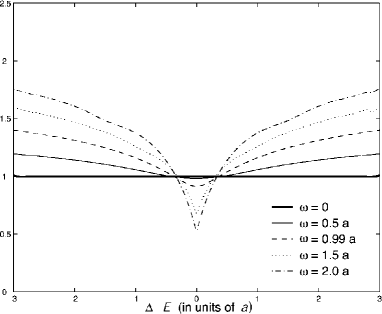
Figure 5: The energy dependent effective temperatures. The temperature is plotted as a function of detector energy for several values of $\omega/a$. It is measured relative to the Unruh temperature $a/2\pi$ defined by the proper acceleration of the accelerated detector.

In Fig.5 we have plotted this function, relative to the Unruh temperature $a/2\pi$, for some values of $\omega/a$ both with $\omega<a$ and $\omega>a$. For moderate values of $\omega/a$ one notes that the energy dependence is not very strong, and this gives support to the idea that the definition of an effective temperature is physically meaningful. Even when $\omega/a$ is larger and increases beyond the value $1$ where the event horizon of the accelerated orbit disappears, there is no dramatic change. Thus, even if in the general case a precise temperature cannot be given, a qualitative description of the effect as heating of the accelerated detector by the vacuum fluctuations seems reasonable, with an effective temperature not very different from the Unruh temperature $a/2\pi$ defined by the acceleration parameter of the orbit.

VI Non-planar motion

We now turn to the general case where the motion is no longer planar and the general form of the Hamiltonian is given by (1) or (2), with $\boldsymbol{a}\cdot\boldsymbol{\omega}\neq 0$. Since this case is qualitatively not so different from the case of planar motion, we will discuss it more briefly. In this case as well, we can simplify the form of the Hamiltonian by a Lorentz transformation. It is now done by transforming the coefficients of the boost operator and the angular momentum to co-linear form. The transformation is, as for planar motion, a boost in the direction orthogonal to both $\boldsymbol{a}$ and $\boldsymbol{\omega}$ (the y-direction).

The transformation of the boost operator and the angular momentum under a Lorentz transformation is

$$\mbox{$$}\boldsymbol{K} = \gamma(\boldsymbol{K}^{\prime}-\boldsymbol{\beta}\times\boldsymbol{J}^{\prime}-\frac{\gamma}{\gamma+1}\boldsymbol{\beta}\;\boldsymbol{\beta}\cdot\boldsymbol{K}^{\prime})$$

$$\boldsymbol{J} = \gamma(\boldsymbol{J}^{\prime}+\boldsymbol{\beta}\times\boldsymbol{K}^{\prime}-\frac{\gamma}{\gamma+1}\boldsymbol{\beta}\;\boldsymbol{\beta}\cdot\boldsymbol{J}^{\prime})$$ (72)

which gives the following expression for the Hamiltonian in terms of operators of the transformed inertial frame,

$$\mbox{$$}H_{O}=\gamma[H^{\prime}+\boldsymbol{\beta}\cdot\boldsymbol{P}^{\prime}-(\boldsymbol{a}-\boldsymbol{\beta}\times\boldsymbol{\omega})\cdot\boldsymbol{K}^{\prime}-(\boldsymbol{\omega}+\boldsymbol{\beta}\times\boldsymbol{a})\cdot\boldsymbol{J}^{\prime}]$$ (73)

for $\boldsymbol{\beta}$ orthogonal to $\boldsymbol{a}$ and $\boldsymbol{\omega}$. The coefficients of the two operators become co-linear if

$$\mbox{$$}\boldsymbol{\beta}=\frac{\boldsymbol{\omega}\times\boldsymbol{a}}{2(\boldsymbol{\omega}\times\boldsymbol{a})^{2}}\big{[}a^{2}+\omega^{2}-\sqrt{(a^{2}-\omega^{2})^{2}+4(\boldsymbol{\omega}\cdot\boldsymbol{a})^{2}}\big{]}$$ (74)

We note that by a further transformation in the form of a shift in the location of the spatial origin, the operator $H^{\prime}$ can be absorbed in $\boldsymbol{K}^{\prime}$ and $\boldsymbol{P}^{\prime}$ can be absorbed in $\boldsymbol{J}^{\prime}$.

We specify the choice of axes for the original frame in the same way as given by (2), with $\boldsymbol{a}$ directed (with value $a$) in the $x$-direction and with $\boldsymbol{\omega}$ as a vector with components $\omega_{x}$ and $\omega_{z}$ in the $x,z$-plane. For the transformed frame we choose the $x^{\prime}$-coordinate to be in the direction of the co-linear boost and axis of rotation, as specified by (73) and (74). This direction is rotated relative to the $x$-axis in the $x,z$-plane. With these choices the Hamiltonian of the accelerated frame gets the form

$$\mbox{$$}H_{O}=\gamma[-\sqrt{(a-\beta\omega_{z})^{2}+\beta^{2}\omega_{x}^{2}}\;K_{x^{\prime}}\pm\sqrt{(\beta a-\omega_{z})^{2}+\omega_{x}^{2}}\;J_{x^{\prime}}]$$ (75)

where $\beta$ is the component of $\boldsymbol{\beta}$ in the direction of $\boldsymbol{\omega}\times\boldsymbol{a}$ as given by (74), $\gamma=(1-\beta^{2})^{-1/2}$ and the relative signs of the two terms is determined by the sign of $\boldsymbol{\omega}\cdot\boldsymbol{a}$.

This form of the accelerated Hamiltonian is not very different from the one given by (35) for planar acceleration with $a>\omega$. The main difference is that the translation operator $P_{y^{\prime}}$ is replaced by the angular momentum operator $J_{x^{\prime}}$. This implies that the accelerated trajectory (of the reference curve $C$), as seen in the transformed frame, now is a superposition of a rotation about the $x^{\prime}$-axis and uniform acceleration in the $x^{\prime}$-direction. It is an accelerated screw-like motion.

In the same way as for planar acceleration, the asymptotic form of the trajectory is dominated by the $x^{\prime}$-component of the motion, and the location of the event horizons is determined by the uniform acceleration of the $x^{\prime}$-projection of the reference curve. The location of the event horizons and static limit in the accelerated frame can be found in the same way as for planar motion, by transformation to the inertial rest frame at time $\tau=0$. The main difference between the two cases is that there is no longer translational invariance in the $z$-direction, so that the corresponding surfaces are curved also in this direction. We do not give explicit expressions for these surfaces, but note that the qualitative picture is the same as before. Between the accelerated observer on the trajectory $C$ and the event horizons there is a static limit, where the stationary curves of the accelerated frame change from being time-like to being space-like. Note that in the present case there is always an event horizon, without any restriction on the values of $a$ and $\omega$.

Since $J_{x^{\prime}}$ commutes with $K_{x^{\prime}}$ the eigenstates of the accelerated Hamiltonian can be chosen as eigenstates of the boost operator, in the same way as for planar motion. The difference is that the $x^{\prime},z^{\prime}$-dependent factor of these states should be angular momentum states and not plane waves. Thus, by a Bogoliubov transformation the field modes that are located behind the horizons, as viewed from the accelerated observer, can be separated out and energy eigenstates restricted to the right Rindler wedge of the boost operator $K_{x^{\prime}}$ can be defined. Also now there will be negative energy states, and these are up to exponentially decaying tails located between the horizon and the static limit. The Minkowski vacuum state, when restricted to the right Rindler wedge, is described by a density matrix which is of the form

$$\mbox{$$}\rho_{M}={\cal N}e^{-\frac{1}{\theta}(H_{O}+\boldsymbol{\Omega}^{\prime}\cdot\boldsymbol{J}^{\prime})}$$ (76)

with $\cal N$ as a normalization factor, $\theta$ and $\boldsymbol{\Omega}^{\prime}$ given by

$$\mbox{$$}\theta = \frac{\gamma}{2\pi}\sqrt{(a-\beta\omega_{z})^{2}+\beta^{2}\omega_{x}^{2}}$$

$$\boldsymbol{\Omega}^{\prime} = \gamma(\boldsymbol{\omega}+\boldsymbol{\beta}\times\boldsymbol{a})$$ (77)

When we again interpret the exponent as a thermodynamic potential, the form suggests that in the accelerated frame the Minkowski vacuum state can now be viewed as a rotating, hot ”vacuum gas”. However, the operator $\boldsymbol{J}^{\prime}$ is a rotation operator in the Rindler coordinate frame and not in the rest frame. If we change to operators of the inertial rest frame and parametrize the density operator $\rho_{M}$ of the Minkowski vacuum state in the same way as we did for planar motion, it gets the form

$$\mbox{$$}\rho_{M}=|{\cal K}|^{2}e^{-\frac{2\pi\gamma}{\sqrt{(a-\beta\omega_{z})^{2}+\beta^{2}\omega_{x}^{2}}}(H_{O}-\beta{\cal P)}}$$ (78)

where the symmetry operator ${\cal P}$ now is given by

$$\mbox{$$}{\cal P}=\frac{1}{\beta}(\boldsymbol{\beta}\cdot\boldsymbol{P}-(\boldsymbol{\beta}\times\boldsymbol{\omega})\cdot\boldsymbol{K}-[(1+\beta^{2})\,\boldsymbol{\omega}+\boldsymbol{\beta}\times\boldsymbol{a}]\cdot\boldsymbol{J})$$ (79)

We note that the expression for the symmetry operator in the planar case is recovered in the limit $\boldsymbol{a}\cdot\boldsymbol{\omega}\rightarrow 0$ (when $a>\omega$).

VII Concluding remarks

We have in this paper examined the “generalized Unruh effect”, which refers to observable vacuum effects in general stationary coordinate frames. Such a stationary frame will be characterized both by acceleration and rotation with respect to an inertial rest frame. In the main part of the paper we have focused on planar motion. For accelerated orbits, event horizons will then exist provided the proper acceleration $a$ dominates the angular velocity $\omega$ as measured in an inertial rest frame.

When event horizons exist, the situation is similar to that of uniform linear acceleration. By mixing in a certain way (Minkowski) creation and annihilation operators in the form of a Bogoliubov transformation, excitations associated with the two sides of the horizons decouple, and a field theory restricted to the “physical” side of the horizons may be defined. Relative to these excitations Minkowski vacuum will contain excitations and can be characterized by a thermodynamical potential which depends on a vacuum temperature as well as a drift velocity of the vacuum.

Although Minkowski vacuum can be interpreted as a thermodynamic state, when viewed in the accelerated frame, a stationary detector will not show an excitation spectrum which can be expressed simply in terms of a Boltzmann factor. There are two reasons for this. The first one is due to the drift (and rotation) of the (thermodynamic) vacuum state. This will give rise to non-universal thermal effects like the ones seen by a detector moving with large speed through a hot gas. The other effect is due to the presence of negative energy quanta which are associated with the region behind the static limit in the accelerated frame. Thus, the detector may be excited either due to emission of negative energy quanta or by absorption of positive energy quanta.

For accelerations with $a<\omega$, the event horizons disappear and the motion can be viewed as uniform circular motion. Although these cases seem qualitatively different from the ones characterized by $a>\omega$, and although Minkowski space no longer can be viewed as a (non-trivial) thermodynamic state, we have demonstrated the smooth transition of the effective (energy dependent) temperature as measured by an accelerated detector, when the parameters are continuously changed from one type of motion to the other.

In the case of stationary, non-planar orbits, which can be viewed as circular motion imposed on uniform linear acceleration, event horizons will always exist, and qualitatively the description of the (generalized) Unruh effect for this type of motion will be similar to that of planar motion with $a>\omega$.

Finally we have pointed to the close relation between the vacuum effects for detectors following general stationary curves in Minkowski space and for stationary detectors close to the event horizons of massive rotating black holes. For planar motion we in the appendix explicitly show how the metric of the accelerated frame is identical to the limiting form of the Kerr metric for points close to the equator of the rotating black hole when the mass of the hole tends to infinity.

VII.1 Acknowledgements

JML thanks the Miller Institute for Basic Research in Science for financial support and hospitality during his visit to UC Berkeley. Supports from the Research Council of Norway and the Fulbright Foundation are also acknowledged.

Appendix A Appendix. Connection between Kerr spacetime and trajectories with $\omega\neq 0$

In this appendix we compare the sitation of a stationary observer close to the static limit of a rotating (Kerr) black hole with that of an accelerated observer in Minkowski space. We show that in the limit where the mass M of the black hole tends to infinity, space-time near the observer becomes flat, and the space-time trajectory becomes identical to a stationary curve in Minkowski space. We restrict the discussion to the case where the observer is located close to the equator of the black hole. In this case the space time curve is a planar stationary curve characterized by a constant proper acceleration $\boldsymbol{a}$ and angular velocity $\boldsymbol{\omega}$, where $\boldsymbol{a}\perp\boldsymbol{\omega}$ and $\boldsymbol{\omega}\neq 0$ and $a>\omega$. As we shall show, the two parameters $a$ and $\omega$ can be related to the parameters of the black hole and the position of the observer. (In the appendix we use $G=1$ for the gravitationol constant (rather than $\hbar=1$) and still use $c=1$ for the speed of light.)

At the equator of a rotating black hole ($\theta=\pi/2$), the Kerr metric expressed in Boyer-Lindquist coordinates gets the following form:

$$\mathrm{d}s^{2}=\left(1-\frac{2M}{r}\right)\mathrm{d}t^{2}-\frac{r^{2}}{r^{2}+j^{2}-2Mr}\mathrm{d}r^{2}-r^{2}\mathrm{d}\theta^{2}\\ \\ -\left(r^{2}+j^{2}+\frac{2Mj^{2}}{r}\right)\mathrm{d}\phi^{2}+\frac{4Mj}{r}\mathrm{d}t\mathrm{d}\phi$$ (80)

where $M$ is the mass of the hole and $j$ is the angular momentum per unit mass of the black hole, usually called $a$ in the literature, but renamed here to avoid confusion with the acceleration parameter. In these coordinates the event horizon is located at $r_{h}=M-\sqrt{M^{2}-j^{2}}$ and the static limit at $r_{s}=2M$.

We now want to show that for a space-time region centered around a static trajectory with fixed coordinates $r>2M,\theta=\pi/2,\phi=0$ (arbitrarily chosen), there exists a mapping between the Boyer-Lindquist coordinates of the black hole and a coordinate system of an accelerated observer in Minkowski space. This mapping becomes an isometry (i.e. it maps the Kerr metric into the metric of the observer following the stationary trajectory) in the limit $M\rightarrow\infty$.

Since we focus on space-time points close to the static limit we write the radial coordinate as

$$\mbox{$$}r=2M+q$$ (81)

with $q$ as a new coordinate to replace $r$. The $M\rightarrow\infty$ limit we assume to be taken in such a way that $q/M\rightarrow 0$ and $j^{2}/M\rightarrow 0$. The last condition is imposed in order for the distance between the static limit and the event horizon to stay finite when $M$ tends to infinity. With these approximations the metric outside the static limit is

$$\mbox{$$}ds^{2}=\frac{q}{2M}dt^{2}-\frac{2M}{q+\frac{j^{2}}{2M}}dq^{2}-4M^{2}d\theta^{2}-4M^{2}d\phi^{2}+2jdtd\phi$$ (82)

and with a rescaling of the coordinates,

$$\mbox{$$}\bar{t}=\frac{t}{2M},\quad\bar{q}=2Mq,\quad\bar{z}=2M\theta,\quad\bar{y}=2M\phi$$ (83)

it further gets the $M$ independent form

$$\mbox{$$}ds^{2}=\bar{q}{d\bar{t}}^{2}-\frac{1}{\bar{q}+j^{2}}d\bar{q}^{2}-d{\bar{z}^{2}}-d\bar{y}^{2}+2jd\bar{t}d\bar{y}$$ (84)

To compare this expression with the Minkowski space metric, as it appears in an accelerated frame with $\omega\neq 0$, we make use of the (accelerated) coordinates (IV.1). In these coordinates the accelerated observer is not stationary, but has a constant drift velocity in the $y$-direction determined by the ratio $\omega/a$. To compensate for the drift we redefine the $y$-coordinate

$$\tilde{y}=y^{\prime}+\frac{\omega}{\sqrt{a^{2}-\omega^{2}}}\,\tau^{\prime}$$ (85)

so that the accelerated observer is stationary in the coordinate system $(\tau^{\prime};\xi^{\prime},\tilde{y},z)$. As previously discussed, the values of the proper acceleration $a$ and the angular velocity $\omega$ fix the $\xi^{\prime}$ coordinate to be $\xi^{\prime}=a/(a^{2}-\omega^{2})$, while the other space coordinates may be chosen as $\tilde{y}=z=0$. We note that the spatial hyperplane defined by these coordinates is not the observer’s plane of simultaneity (as it is for the accelerated coordinates $(\tau;\xi,\eta,z)$ previously used), since the coordinates are not static. However, this is not a problem, since the same thing is true of the Boyer-Lindquist coordinates.

In the coordinates $(\tau^{\prime};\xi^{\prime},\tilde{y},z)$, the Minkowski space metric takes the form

$$\mathrm{d}s^{2}=\left(a^{2}-\omega^{2}\right)\left({\xi^{\prime}}^{2}-\frac{\omega^{2}}{\left(a^{2}-\omega^{2}\right)^{2}}\right)\,\mathrm{d}{\tau^{\prime}}^{2}-\mathrm{d}{\xi^{\prime}}^{2}-\mathrm{d}\tilde{y}^{2}-dz^{2}-\frac{2\omega}{\sqrt{a^{2}-\omega^{2}}}\,\mathrm{d}\tilde{y}\,\mathrm{d}\tau^{\prime}$$ (86)

This can be recast in a form similar to (84) by redefining the coordinates. Thus, if we make the following identifications between coordinates

$$\mbox{$$}\bar{q} = \frac{1}{4}({\xi^{\prime}}^{2}-\frac{\omega^{2}}{\left(a^{2}-\omega^{2}\right)^{2}})$$

$$\bar{t} = 2\sqrt{a^{2}-\omega^{2}}\tau^{\prime}$$

$$\bar{y} = \tilde{y}$$

$$\bar{z} = z$$ (87)

and if we identify $2j$ with the following function of $a$ and $\omega$,

$$\mbox{$$}2j=\frac{\omega}{a^{2}-\omega^{2}}$$ (88)

then (86) reproduces exactly the metric (84) derived from the black hole metric.

We note that the angular momentum parameter of the black hole, $2j=\omega/(a^{2}-\omega^{2})\equiv d_{hs}$, can also be interpreted as the distance between the event horizon and the static limit, as measured in the instantaneous rest frame of the stationary observer. This follows from the expressions (41) and (44) for the location of the horizon and static limit in the accelerated frame. In the same way $a/(a^{2}-\omega^{2})\equiv d_{ho}$ measures the distance from the observer to the event horizon. Thus the dimensionless ratio $\omega/a$ corresponds to the ratio between these two distances, and the limiting value $\omega/a\rightarrow 1$ can be obtained by making $j$ large compared to the distance between the static observer and the static limit.

In conclusion, we have shown how to map the coordinate system near a stationary observer, located outside the static limit of a rotating black hole, to a Minkowski space coordinate system where an accelerated observer is at rest, and to show that in the limit $M\rightarrow\infty$ the mapping is an isometry. The two parameters $a$ and $\omega$ of the accelerated orbit we have related to the angular momentum $j$ of the black hole and the distance from the static observer to the event horizon.

The mapping between these two seemingly different situations indicates that the (generalized) Unruh effect associated with motion along stationary space-time curves in Minkowski space is of similar form as the effect measured by a stationary detector outside the stationary limit of a massive rotating black hole. However, a more detailed discussion of this point depends on showing in what sense the Minkowski vacuum state is the natural vacuum state of the black hole in the limit $M\rightarrow\infty$.

References

- (1) W. G. Unruh, Phys. Rev. D 14, 870 (1976)
- (2) S. A. Fulling, Phys. Rev. D 7, 2850 (1973)
- (3) P. C. W. Davies, J. Phys. A 8, 609 (1975)
- (4) S. W. Hawking, Nature 248, 30 (1974)
- (5) S. W. Hawking, Commun. Math. Phys. 43, 199 (1975)
- (6) J. R. Letaw and J. D. Pfautsch, Phys. Rev. D 24, 1491 (1981)
- (7) J. R. Letaw, Phys. Rev. D 23, 1709 (1981)
- (8) J. S. Bell and J. M. Leinaas, Nucl. Phys. B 212, 131 (1983)
- (9) J. S. Bell and J. M. Leinaas, Nucl. Phys. B 284, 488 (1987)
- (10) W.G. Unruh, Acceleration Radiation for Orbiting Electrons, in Quantum Aspects of Beam Physics (Monterey 1998), Ed. Pisin Chen, World Scientific 1999.
- (11) J.M. Leinaas Unruh effect in storage rings, in Quantum Aspects of Beam Physics (Capri 2000), Ed. Pisin Chen, World Scientific 2002.
- (12) I. Rogers, Phys. Rev. Lett. 61, 2113 (1988).
- (13) O. Levin, Y Peleg and A Peres, J. Phys. A: Math. Gen. 26, 3001 (1993).
- (14) P.C.W. Davies, T. Dray and C. Manogue, Phys. Rev. D 53, 4382 (1996).
- (15) G. Sewell, Ann. Phys. (N.Y.) 141, 201(1982).
- (16) R.J. Hughes, Ann. Phys. (N.Y.) 162, 1(1985).
- (17) J.S. Bell, R.J. Hughes and J.M. Leinaas, Zeit. f Physik 28, 75 (1985).
- (18) J.S. Bell, Proc. R. Soc. London Ser. A 231, 479 (1955).
- (19) W. Rindler, Am. J. Phys. 34, 1174 (1966).
- (20) J. M. Bardeen, B. Carter and S. W. Hawking, Commun. Math. Phys. 31, 161 (1973)
- (21) E. C. Titchmarsh, Eigenfunction Expansions, Oxford University Press 1958, Vol. I
- (22) R. Penrose, Rivista Del Nuovo Cimento: Numero Speciale 1, 252 (1969).
- (23) U. H. Gerlach, Phys. Rev. D 27, 2310 (1983)
- (24) Even for linear acceleration one may note an ambiguity in associating a specific temperature with the vacuum state as viewed in the accelerated Rindler coordinates. The temperature corresponds to the local temperature measured at the position of the reference curve , while at other points in the accelerated frame the temperature will be different. This is similar to the situation in a gravitational field, where the specification of a temperature of a hot gas will depend on a choice of a reference point, since the locally measured temperature will vary in space due to the redshift effect.
- (25) The change introduced in the Hamiltonian can be viewed as due to a gravitational effect of the rotation.
- (26) N. D. Birrell and P. C. W. Davies, Quantum Fields in Curved Space, Cambridge University Press 1982