Abstract

We investigate the structure of the higher genus topological string amplitudes on the quintic hypersurface. It is shown that the partition functions of the higher genus than one can be expressed as polynomials of five generators. We also compute the explicit polynomial forms of the partition functions for genus 2, 3, and 4. Moreover, some coefficients are written down for all genus.

1 Introduction

The topological string theory on a Calabi-Yau 3-fold is a good toy model as well as a computational tool of the superstring. Especially, it is a practicable problem to calculate the higher genus amplitudes, while those of the physical string are technically difficult to calculate. The topological A-model partition functions on a Calabi-Yau 3-fold $M$ is defined for genus $g\geq 2$ as

$$F^{\text{A-model}}_{g}(t)=\sum_{d\in H_{2}(M,\mathbb{Z})}e^{-d\cdot t}\int_{\overline{\cal M}_{g,d}}1,$$ (1.1)

where $\overline{\cal M}_{g,d}$ is the compactified moduli space of degree $d$ holomorphic map from genus $g$ Riemann surface to $M$, and $t$ is a vector of complexified Kähler parameters. In the physical view point, the partition function can be defined similar way to the bosonic string as follows. Let us consider the A-twisted theory of the sigma model on the Calabi-Yau $M$. It becomes a $N=2$ topological CFT which depends on the Kähler parameter $t$. We denote by ${\cal M}_{g}$ the moduli space of the complex structure on genus $g$ Riemann surface. Then the genus $g\geq 2$ topological string partition function can be defined as

$$F_{g}(t,\bar{t})=\int_{{\cal M}_{g}}\left\langle\prod_{k=1}^{3g-3}\left(\int G^{-}\mu_{k}\right)\left(\int\bar{G}^{-}\bar{\mu}_{k}\right)\right\rangle_{g,t},$$ (1.2)

where $\mu_{k}$’s are the Beltrami differentials and $G^{-},\bar{G}^{-}$ are “$b$-ghosts” of $N=2$ topological CFT. The two definition are connected by a gauge transformation $f(t)$ and the limit, namely

$$F_{g}^{\text{A-model}}(t)=\lim_{\bar{t}\to\infty}f(t)^{2-2g}F_{g}(t,\bar{t}).$$ (1.3)

The non-holomorphic partition function $F_{g}(t,\bar{t})$ has a good global properties.

The $\bar{t}$ dependence is governed by the holomorphic anomaly equation which is written down by Bershadsky, Cecotti, Ooguri and Vafa [1, 2]. This equation provides an effective method to calculate the higher genus amplitudes. But there remain some ambiguities to determine the amplitudes by using the holomorphic anomaly equation. Ref. [2] have used geometric consideration to fix the ambiguity, and obtain genus 2 partition function for the quintic hypersurface. As Ghoshal and Vafa have pointed out in [3], comparing the conifold limit and the topological string on conifold gives non-trivial information. In [4], Katz, Klemm, and Vafa have used the M-theory picture and obtained genus 3 and 4 partition function for the quintic. In order to proceed this calculation, we want to understand the structure of the higher genus amplitudes.

Higher genus amplitudes are expected to have the property similar to the modular forms. Every modular form can be written in a quasi-homogeneous polynomial of Eisenstein series $E_{4}$ and $E_{6}$. This is the very beginning of the interesting theory of the modular forms. It will be interesting as well as useful if the topological string partition function has this kind of polynomial structure. Actually, as pointed out in [5], a discrete group similar to $SL(2,Z)$ but not the same, act to the moduli space of the quintic hypersurface.

In this paper, we explore the structure of the higher genus amplitudes of the quintic hypersurface. We will show that the topological string partition function $F_{g}$ can be written as a degree $(3g-3)$ quasi-homogeneous polynomial of five generators $V_{1},V_{2},V_{3},W_{1},Y_{1}$, where we assign the degree $1,2,3,1,1$ for $V_{1},V_{2},V_{3},W_{1},Y_{1}$ , respectively. The generators $V_{1},V_{2},V_{3},W_{1},Y_{1}$ are the functions of the moduli parameter whose explicit forms are summarized in eqs.(3.33).

This fact provides a simple expression of the partition function of each genus; This polynomial expression is completely closed and includes all the data of the coefficients of instanton expansion. The polynomial is also more compact than the raw Feynman diagram expression; The number of terms grows only in power of the genus.

The construction of this paper is as follows. In section 2, we review the method of calculation of topological string amplitudes by using the mirror symmetry and the holomorphic anomaly equation. In section 3, we prove that the partition function can be written as a polynomial of the five generators. Some of the coefficients are calculated in section 4. Section 5 is devoted to conclusions and discussions. In appendix A, polynomial form of genus 3 and 4 partition function are written. In appendix B, we discuss the generalization to the Calabi-Yau hypersurfaces in weighted projective spaces treated in [6].

2 Calculation of topological string amplitudes by mirror symmetry and the holomorphic anomaly equation

In this section, we review the calculation of the topological string amplitudes by the mirror symmetry[5, 1, 2]. First, we explain the genus zero amplitudes following [5]. After that, we will explain the genus one amplitudes and the higher genus ones following [1, 2]. In this paper, we mainly work with the quintic hypersurface in $\mathbb{C}P^{4}$. For this reason, we will concentrate to the case of quintic in the review in this section.

2.1 Genus zero

Let us review the genus zero amplitudes of the quintic[5]. The mirror manifold of the quintic is expressed by the orbifold of the hypersurface in $\mathbb{C}P^{4}$[7]

$$p:=x_{1}^{5}+x_{2}^{5}+x_{3}^{5}+x_{4}^{5}+x_{5}^{5}-5\psi x_{1}x_{2}x_{3}x_{4}x_{5}=0,$$ (2.1)

where $x_{j},\ j=1,2,3,4,5$ are the homogeneous coordinates of $\mathbb{C}P^{4}$, and $\psi$ is the moduli parameter. The orbifold group is $(\mathbb{Z}_{5})^{3}$ . If we denote the generators of this $(\mathbb{Z}_{5})^{3}$ by $g_{1},g_{2},g_{3}$, the action can be written as

$$g_{j}:x_{j}\to e^{\frac{2\pi i}{5}}x_{j},\quad x_{5}\to e^{\frac{-2\pi i}{5}}x_{5},\quad x_{i}\to x_{i},\ (i\neq j,5).$$ (2.2)

We fix the gauge to the standard one in which the holomorphic 3-form $\Omega$ is written as

$$\Omega=5\psi\frac{x_{5}dx_{1}\wedge dx_{2}\wedge dx_{3}}{\partial p/\partial x_{4}}.$$ (2.3)

In this gauge, the Picard-Fuchs equation for a period $w=\int\Omega$ is given by

$$\left\{\left(\psi\partial_{\psi}\right)^{4}-\psi^{-5}\left(\psi\partial_{\psi}-1\right)\left(\psi\partial_{\psi}-2\right)\left(\psi\partial_{\psi}-3\right)\left(\psi\partial_{\psi}-4\right)\right\}w=0.$$ (2.4)

There is a solution $\omega_{0}$ which is regular at $\psi\to\infty$. This solution is expressed by the expansion in $\psi^{-5}$ as

$$\omega_{0}(\psi)=\sum_{n=0}^{\infty}\frac{(5n)!}{(n!)^{5}(5\psi)^{5n}}.$$ (2.5)

In order to write down the other solutions, we extend the definition of $\omega_{0}$ to the function of $\psi$ and $\rho$ to use the Frobenius argument. This function $\omega_{0}(\psi,\rho)$ should be the form

$$\omega_{0}(\psi,\rho)=\sum_{n=0}^{\infty}\frac{\Gamma(5(n+\rho)+1)}{\Gamma(n+\rho+1)^{5}(5\psi)^{5(n+\rho)}}.$$ (2.6)

The natural basis of the solutions are written as

$$\Pi=\left.\left(\begin{array}[]{c}w_{0}\\ w_{1}\\ \partial_{1}F_{0}\\ \partial_{0}F_{0}\end{array}\right)=\left(\frac{2\pi i}{5}\right)^{3}\left(\begin{array}[]{c}\omega_{0}(\psi,\rho)\\ \frac{1}{2\pi i}\partial_{\rho}\omega_{0}(\psi,\rho)\\ \frac{5}{2}\left(\frac{1}{2\pi i}\partial_{\rho}\right)^{2}\omega_{0}(\psi,\rho)\\ -\frac{5}{6}\left(\frac{1}{2\pi i}\partial_{\rho}\right)^{3}\omega_{0}(\psi,\rho)\end{array}\right)\right|_{\rho=0}\;.$$ (2.15)

This basis are standard symplectic basis. Therefore, the Kähler potential $K$ of the moduli space can be written as

$$e^{-K}=-i\Pi^{{\dagger}}\Sigma\Pi,\qquad\Sigma=\left(\begin{array}[]{cccc}0&0&0&1\\ 0&0&1&0\\ 0&-1&0&0\\ -1&0&0&0\\ \end{array}\right).$$ (2.20)

This matrix $\Sigma$ is the ordinary symplectic bilinear form. The metric of the moduli space is obtained as $G_{\psi\bar{\psi}}=\partial_{\psi}\bar{\partial}_{\bar{\psi}}K$.

Let us denote the complexified Kähler parameter in the A-model picture by $t$. The relation between $\psi$ and $t$ (“mirror map”) is given by

$$t=-2\pi i\frac{w_{1}}{w_{0}}=-\log(5\psi)^{-5}-\frac{5}{\omega_{0}}\sum_{m=1}^{\infty}\frac{(5m)!}{(m!)^{5}(5\psi)^{5m}}(\Psi(1+5m)-\Psi(1+m)),$$ (2.21)

where $\Psi(x):=\partial_{x}\log\Gamma(x)$ .

Another important observable is the Yukawa coupling. It is determined by

$$C_{\psi\psi\psi}=\Pi^{T}\Sigma\partial_{\psi}^{3}\Pi.$$ (2.22)

This equation and the Picard-Fuchs equation read the following differential equation for the Yukawa coupling.

$$\partial_{\psi}C_{\psi\psi\psi}=\frac{2\psi^{-1}+4\psi^{3}}{1-\psi^{5}}C_{\psi\psi\psi}.$$ (2.23)

This differential equation can be solved as

$$C_{\psi\psi\psi}=\frac{(2\pi i)^{3}}{5^{3}}\frac{\psi^{2}}{1-\psi^{5}},$$ (2.24)

where the normalization is fixed by the asymptotic behavior. The Yukawa coupling in the $t$-frame becomes

$$C^{\text{A-model}}_{ttt}=\left(\frac{(2\pi i)^{3}}{5^{7}}\omega_{0}^{2}\right)^{-1}\left(\frac{\partial\psi}{\partial t}\right)^{3}C_{\psi\psi\psi}.$$ (2.25)

The first factor in the right-hand side comes from the gauge transformation, and the second factor is the contribution of the coordinate transformation. The $C^{\text{A-model}}_{ttt}$ gives the instanton expansion of the A-model picture and includes the information of the number of rational curves in the quintic.

These quantities, Kähler potential, metric, and Yukawa coupling are essential to compute the higher genus amplitudes.

2.2 Genus one and higher

The one point function $\partial_{\psi}F_{1}$ of genus one satisfies the holomorphic anomaly equation[1]

$$\bar{\partial}_{\bar{\psi}}\partial_{\psi}F_{1}=\frac{1}{2}C_{\psi\psi\psi}\overline{C}_{\bar{\psi}}^{\psi\psi}-\left(\frac{\chi}{24}-1\right)G_{\psi\bar{\psi}},\qquad\chi=-200,$$ (2.26)

where $\overline{C}_{\bar{\psi}}^{\psi\psi}$ is defined as

$$\overline{C}_{\bar{\psi}}^{\psi\psi}:=\overline{C}_{\bar{\psi}\bar{\psi}\bar{\psi}}(G_{\psi\bar{\psi}})^{-2}e^{2K}.$$ (2.27)

Eq. (2.26) can be solved as

$$\partial_{\psi}F_{1}=\frac{1}{2}\partial_{\psi}\log\left[(G_{\psi\bar{\psi}})^{-1}\exp\left(\frac{62}{3}K\right)\psi^{62/3}(1-\psi^{5})^{-1/6}\right].$$ (2.28)

The holomorphic ambiguity is fixed by the asymptotic behavior. In the $t$-frame, and topological limit ($\bar{t}\to\infty$), this one point function becomes

$$\partial_{t}F^{\text{A-model}}_{1} =\lim_{\bar{t}\to\infty}\frac{\partial\psi}{\partial t}\partial_{\psi}F_{1}.$$ (2.29)

This function gives the instanton expansion in A-model picture, and includes the information of the number of elliptic curves in the quintic.

Let us turn to the $g\geq 2$ amplitudes. First, we introduce some notations. We denote the vacuum bundle by $L$. Holomorphic 3-form $\Omega$ is a section of $L$. For a section of $L$, the action of the gauge transformation (Kähler transformation) are parametrized by a holomorphic function $f(\psi)$ and expressed as

$$K(\psi,\bar{\psi})\to K(\psi,\bar{\psi})-\log f(\psi)-\log\bar{f}(\bar{\psi}),\qquad\Omega\to f(\psi)\Omega.$$ (2.30)

The genus $g$ partition function $F_{g}$ is a section of $L^{2-2g}$ and transform as $F_{g}\to f(t)^{2-2g}F_{g}$. Besides this symmetry of Kähler transformation, there is another gauge symmetry — the reparametrization of the moduli. We will define the covariant derivative $D_{\psi}$ for these two gauge transformations. If $h(\psi)$ is a section of $(T^{*})^{m}\otimes L^{n}$, the covariant derivative of $h$ is defined as

$$D_{\psi}h=\partial_{\psi}h+m\Gamma^{\psi}_{\psi\psi}h+n(\partial_{\psi}K)h,$$ (2.31)

where $\Gamma^{\psi}_{\psi\psi}=-(G_{\psi\psi})^{-1}\partial_{\psi}G_{\psi\psi}$ is the Christoffel symbol.

Next, we consider the holomorphic anomaly equation. The holomorphic anomaly equation for the genus $g$ partition function $F_{g}$ is given by [2]

$$\bar{\partial}_{\bar{\psi}}F_{g}=\frac{1}{2}\overline{C}_{\bar{\psi}}^{\psi\psi}\left(D_{\psi}D_{\psi}F_{g-1}+\sum_{r=1}^{g-1}D_{\psi}F_{\psi}D_{\psi}F_{g-r}\right).$$ (2.32)

A solution of (2.32) is given by the Feynman rule as in [2]. We denote this solution by $F_{g}^{(FD)}$. The Feynman rule is composed of two kind of things: propagators and vertices. We begin with the propagators. It is useful to introduce the following quantities.

$$S^{\psi\psi}=\frac{1}{C_{\psi\psi\psi}}[2\partial_{\psi}\log(e^{K}|f|^{2})-\partial_{\psi}\log(|v|^{2}G_{\psi\bar{\psi}})],$$ (2.33a)

$$S^{\psi}=\frac{1}{C_{\psi\psi\psi}}\left[\left(\partial_{\psi}\log(e^{K}|f|^{2})\right)^{2}-v^{-1}\partial_{\psi}\left(v\partial_{\psi}\log(e^{K}|f|^{2})\right)\right],$$ (2.33b)

$$S=\left[S^{\psi}-\frac{1}{2}D_{\psi}S^{\psi\psi}-\frac{1}{2}(S^{\psi\psi})^{2}C_{\psi\psi\psi}\right]\partial_{\psi}\log(e^{K}|f|^{2})+\frac{1}{2}D_{\psi}S^{1}+\frac{1}{2}S^{\psi\psi}S^{\psi}C_{\psi\psi\psi},$$ (2.33c)

where $f$ is a holomorphic section of $L$ and $v$ is a holomorphic vector field on the moduli space. In our gauge, we can set $f=\psi$ and $v=1$. The quantities $S^{\psi\psi},S^{\psi},S$ in (2.33) are determined to satisfy the relations

$$\overline{C}_{\bar{\psi}}^{\psi\psi}=\bar{\partial}_{\bar{\psi}}S^{\psi\psi},\qquad S^{\psi\psi}=(G_{\psi\bar{\psi}})^{-1}\bar{\partial}_{\bar{\psi}}S^{\psi},\qquad S^{\psi}=(G_{\psi\bar{\psi}})^{-1}\bar{\partial}_{\bar{\psi}}S.$$ (2.34)

To show these relations, we use the special geometry relations[8]

$$\begin{split}\bar{\partial}_{\bar{\psi}}C_{\psi\psi\psi}=0,\qquad\partial_{\psi}\overline{C}_{\psi\psi\psi}=0,\\ R_{\psi\bar{\psi}\psi}{}^{\psi}:=-\bar{\partial}_{\bar{\psi}}\Gamma^{\psi}_{\psi\psi}=2G_{\psi\bar{\psi}}-C_{\psi\psi\psi}\overline{C}_{\bar{\psi}}^{\psi\psi}.\end{split}$$ (2.35)

There are three types of propagators; The one connecting two solid lines, the one connecting solid and dashed lines, and the one connecting two dashed lines. The value of these propagators are written as

$$\includegraphics[width=56.9055pt]{solidline.eps}=-S^{\psi\psi},\qquad\includegraphics[width=56.9055pt]{halfdashed.eps}=-S^{\psi},\qquad\includegraphics[width=56.9055pt]{dashed.eps}=-2S.$$ (2.36)

Let us turn to the vertices. A vertex is labeled by three integers $g,n,m$. $n$ solid lines and $m$ dashed lines end to the vertex labeled by $g,n,m$. We denote the value of the vertex as

$$\begin{minipage}{113.81102pt} \includegraphics[width=99.58464pt]{vertex.eps} \end{minipage}=\lambda^{2g-2+n+m}\widetilde{C}^{(g)}_{\psi^{n},\varphi^{m}},$$ (2.37)

where $\lambda$ is the topological string coupling constant. The detail of the vertex $\widetilde{C}^{(g)}_{\psi^{n},\varphi^{m}}$ are described as

$$\begin{split}\widetilde{C}^{(g)}_{\psi^{n},\varphi^{m+1}}=(2g-2+n+m)\widetilde{C}^{(g)}_{\psi^{n},\varphi^{m}},\qquad\widetilde{C}^{(g)}_{\psi^{n},\varphi^{0}}=C^{(g)}_{\psi^{n}},\ (2g-2+n\geq 1),\\ C^{(g)}_{\psi^{n}}=D_{\psi}^{n}F_{g},\ (g\geq 2),\qquad C^{(1)}_{\psi^{n}}=D_{\psi}^{n-1}\partial_{\psi}F_{1},\qquad C^{(0)}_{\psi^{n}}=D_{\psi}^{n-3}C_{\psi\psi\psi}\\ \widetilde{C}^{(1)}_{\varphi}=\frac{\chi}{24}-1,\quad\widetilde{C}^{(1)}_{\psi^{0}}=0,\qquad\widetilde{C}^{(0)}_{\psi\psi\varphi^{m}}=\widetilde{C}^{(0)}_{\psi\varphi^{m}}=\widetilde{C}^{(0)}_{\varphi^{m}}=0.\end{split}$$ (2.38)

The value of a diagram is obtained by multiplying the values of all the elements. For example, the following diagram is the one which contribute to $F_{5}$. We can evaluate this diagram as

$$\begin{minipage}{99.58464pt} \includegraphics[width=85.35826pt]{dia.eps} \end{minipage}=\lambda^{8}\widetilde{C}^{(2)}_{\psi,\varphi}\widetilde{C}^{(0)}_{\psi\psi\psi}\widetilde{C}^{(1)}_{\psi,\varphi\varphi}(-S^{\psi\psi})^{2}(-S^{\psi})(-2S).$$ (2.39)

The Feynman diagram part of the partition function is the sum of all connected diagrams ${\cal D}$ divided by the appropriate symmetric factor (constant) $s_{{\cal D}}$

$$F^{(FD)}_{g}\lambda^{2g-2}=-\sum_{\begin{subarray}{c}{\cal D}:\text{connected diagrams}\\ \text{of order $\lambda^{2g-2}$}\end{subarray}}s_{{\cal D}}^{-1}\;{\cal D}.$$ (2.40)

Here, the symmetric factor $s_{{\cal D}}$ is the order of the symmetry group of the diagram ${{\cal D}}$. For example, figure 1 is a diagram which contribute to $F_{4}$. The symmetric factor is counted as follows; factor $2$ from the exchange of the two ends of the line $a$, factor $2$ from the exchange of the two ends of the line $e$, factor $3!$ from the interchange of the three lines $b,c,d$, and factor $2$ from the left-right flip. The symmetric factor becomes $s_{\cal D}=2\times 2\times 3!\times 2=48$.

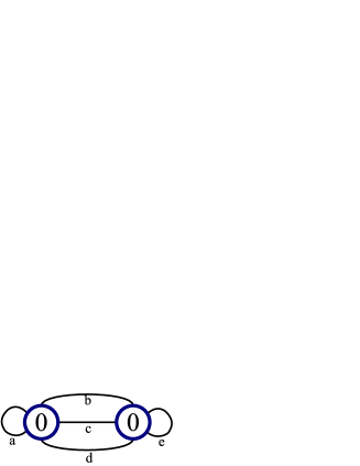
Figure 1: A diagram which contribute to $F_{4}$ the symmetric factor is $s_{\cal D}=2\times 2\times 3!\times 2=48$.

Finally let us mention the holomorphic part. The general solution of the holomorphic anomaly equation (2.32) is

$$F_{g}(\psi,\bar{\psi})=F_{g}^{(FD)}(\psi,\bar{\psi})+f_{g}(\psi),$$ (2.41)

where $f_{g}(\psi)$ is a holomorphic function. From the asymptotic behavior, $f_{g}(\psi)$ can be written as the following form.

$$f_{g}(\psi)=\sum_{j=1}^{[(2g-2)/5]}b_{g,j}\frac{1}{\psi^{5j}}+\sum_{j=0}^{2g-2}a_{g,j}\frac{1}{(1-\psi^{5})^{j}}.$$ (2.42)

Here $[\cdot]$ denotes the Gauss symbol. The coefficients $b_{g,j}$ are determined to cancel the singularity at $\psi=0$. On the other hand, coefficients $a_{g,j}$ are ambiguities and should be determined by other information.

The expression of a partition function in the $t$-frame is given by

$$F_{g}^{\text{A-model}}=\lim_{\bar{t}\to\infty}\left(\frac{(2\pi i)^{3}}{5^{7}}\omega_{0}^{2}\right)^{g-1}F_{g}.$$ (2.43)

By expanding $F_{g}^{\text{A-model}}$ in terms of $e^{-t}$, we will obtain the instanton expansion of the A-model.

3 Generators for the higher genus amplitudes

In this section, we will show that the higher genus amplitudes are expressed as polynomials of finite number of generators. First, in subsection 3.1 we introduce infinite number of generators, and show that the amplitudes can be written as polynomials of these generators. Second, in subsection 3.2, these infinite number of generators turn out to be written as polynomials of finite number of generators. Finally, in section 3.3, we will reconsider the holomorphic anomaly equation and show that the number of generators for partition functions reduces by one. We also state the final form of the claim in the $t$-frame.

3.1 Expression of amplitudes by infinite number of generators

Let us introduce some notations.

$$A_{p}:=\frac{(\psi\partial_{\psi})^{p}G_{\psi\bar{\psi}}}{G_{\psi\bar{\psi}}},\qquad B_{p}:=\frac{(\psi\partial_{\psi})^{p}e^{-K}}{e^{-K}},\qquad(p=1,2,3,\dots),$$

$$C:=C_{\psi\psi\psi}\psi^{3},\qquad X:=\frac{1}{1-\psi^{5}}.$$ (3.1)

Especially, $A:=A_{1}$ and $B:=B_{1}$ are “connections” as

$$A:=A_{1}=-\psi\Gamma^{\psi}_{\psi\psi},\qquad B:=B_{1}=-\psi\partial_{\psi}K.$$ (3.2)

We also denote amplitudes in “(Yukawa coupling)$=1$ frame” by

$$P_{g}:=C^{g-1}F_{g},\qquad P_{g}^{(n)}=C^{g-1}\psi^{n}C^{(g)}_{\psi^{n}},$$ (3.3)

where $P_{g}$ is defined for $g\geq 2$ and $P^{(n)}_{g}$ is defined for $g=0$ and $n\geq 3$, $g=1$ and $n\geq 1$, or $g\geq 2$ and $n\geq 0$. The first thing we want to show is

Proposition 1

Each $P_{g}^{(n)}$ is an degree $(3g-3+n)$ inhomogeneous polynomial of $A_{p},B_{p},X,\ (p=1,2,3,\dots)$, where we assign “degree” $p$ to $A_{p}$ and $B_{p}$, and $1$ to $X$.

Now, we prove this statement. As preliminaries, we consider two things: the derivatives of generators and the expression of propagators. The derivatives of the quantities of eq.(3.1) becomes

$$\psi\partial_{\psi}A_{p}=A_{p+1}-AA_{p},\quad\psi\partial_{\psi}A_{p}=A_{p+1}-AA_{p},\quad\psi\partial_{\psi}X=5X(X-1),\quad\psi\partial_{\psi}C=5XC.$$ (3.4)

We find two facts from these equations. First, if $h(A_{p},B_{p},X)$ is a polynomial of $A_{p},B_{p},X$, then the derivative $\psi\partial_{\psi}h$ is again a polynomial of $A_{p},B_{p},X$. Second, the derivative $\psi\partial_{\psi}$ increases the degree by $1$ in general. We can derive the similar facts for the covariant derivative $\psi D_{\psi}$. Let $h$ be a section of $(T^{*})^{\ell}\otimes L^{m}$, and assume $\psi^{\ell}C^{-m/2}h$ is a polynomial of $A_{p},B_{p},X$ of degree $n$. Then the covariant derivative (2.31) of $h$ becomes

$$C^{-m/2}\psi^{\ell+1}D_{\psi}h=\psi\partial_{\psi}(\psi^{\ell}C^{-m/2}h)+[-\ell(A+1)-m(B-\frac{5}{2}X)](\psi^{\ell}C^{-m/2}h),$$ (3.5)

and therefore $C^{-m/2}\psi^{\ell+1}D_{\psi}h$ is a polynomial of $A_{p},B_{p},X$ of degree $(n+1)$ .

We can write the propagators in eqs. (2.33) in terms of $A_{p},B_{p},X$ as

$$\begin{split}T^{\psi\psi}:=&\frac{C}{\psi^{2}}S^{\psi\psi}=2-2B-A,\qquad T^{\psi}:=\frac{C}{\psi}S^{\psi}=2-3B+B_{2},\\ T:=CS=&\frac{1}{2}\big{[}2+2A+A_{2}-3B-A_{2}B-B^{2}-2AB^{2}+2B^{3}+4B_{2}-\\ &\qquad 5BB_{2}+B_{3}-5AX-5BX+5ABX+10B^{2}X-5B_{2}X\big{]}.\end{split}$$ (3.6)

These equations explicitly shows that $T^{\psi\psi},T^{\psi},T$ are inhomogeneous polynomials of degree $1,2,3$ respectively.

Let us prove proposition 1 by induction. If we assume $P_{g}^{(n)}$ is a polynomial of $A_{p},B_{p},X$ of degree $3g-3+n$, then $P_{g}^{(n+1)}$ can be written as

$$P_{g}^{(n+1)}=\psi\partial_{\psi}P_{g}^{(n)}+[-n(A+1)-(2-2g)(B-\frac{5}{2}X)]P_{g}^{(n)},$$ (3.7)

and $P_{g}^{(n+1)}$ turn out to be a polynomial of degree $(3g-3+n+1)$. As for $g=0$, because $P^{(3)}_{g=0}=1$ by definition, we can conclude that each $P^{(n)}_{g=0},\ n=3,4,5,\dots$ is a polynomial of degree $(-3+n)$. In the case of $g=1$, eq. (2.28) reads

$$P^{(1)}_{g=1}=\frac{31}{3}(1-B)+\frac{5}{12}(X-1)-\frac{1}{2}A,$$ (3.8)

and we also find that each $P^{(n)}_{g=1},\ (n=1,2,3,\dots)$ is a polynomial of degree $n$.

Let us fix $g\geq 2$ and assume each $P^{(n)}_{r},\ r<g$ is a polynomial of degree $(3r-3+n)$. In order to show $P_{g}$ to be a polynomial, we pick up a diagram ${\cal D}$ which contribute to $F_{g}$. We denote the number of vertices by $k$, the number of solid lines by $e$, the number of half-dashed lines by $e^{\prime}$, and the number of dashed lines by $e^{\prime\prime}$ in the diagram ${\cal D}$. We label each vertex by $j,\ (j=1,\dots,k)$ and let the genus of the vertex be $g_{j}$. We also let $n_{j}$ solid lines and $m_{j}$ dashed lines end on the $j$-th vertex. Then considering the number of lines, we find the relations

$$\sum_{j=1}^{k}n_{j}=2e+e^{\prime},\qquad\sum_{j=1}^{k}m_{j}=e^{\prime}+2e^{\prime\prime}.$$ (3.9)

Since ${\cal D}$ contribute to $F_{g}$, we obtain the relation by counting the order of $\lambda$.

$$\sum_{j=1}^{k}(g_{j}-1)+e+e^{\prime}+e^{\prime\prime}=g-1.$$ (3.10)

By using these relations and the expressions of vertices and propagators (2.38), (3.6), ${\cal D}$ is evaluated as

$${\cal D} =(\text{constant})\times\lambda^{2g-2}\left(\prod_{j=1}^{k}\tilde{C}^{(g_{j})}_{\psi^{n_{j}},\varphi^{m_{j}}}\right)(S^{\psi\psi})^{e}(S^{\psi})^{e^{\prime}}(S)^{e^{\prime\prime}}$$

$$=(\text{constant})\times\lambda^{2g-2}\frac{1}{C^{g-1}}\left(\prod_{j=1}^{k}P_{g_{j}}^{(n_{j})}\right)(T^{\psi\psi})^{e}(T^{\psi})^{e^{\prime}}(T)^{e^{\prime\prime}}.$$ (3.11)

$T^{\psi\psi},T^{\psi},T$ are polynomials of $A_{p},B_{p},X$ because of eqs.(3.6), and $P_{r_{j}}^{(n_{j})}$’s are also polynomials due to the assumption of induction. Consequently, $C^{g-1}{\cal D}$ is a polynomial. Its degree is evaluated by using eqs.(3.9),(3.10) as

$$\sum_{j=1}^{k}(3g_{j}-3+n_{j})+e+2e^{\prime}+3e^{\prime\prime}=3g-3.$$ (3.12)

As a result, we can conclude that $C^{g-1}{\cal D}$ is a polynomial of $A_{p},B_{p},X$ of degree $(3g-3)$.

So far, we have shown that the Feynman diagram part of $P_{g}$ is a degree $(3g-3)$ polynomial. Now let us turn to the holomorphic part. Eq. (2.42) is written by using $X$ as

$$f_{g}(\psi)=\sum_{j=1}^{[(2g-2)/5]}b_{g,j}\left(\frac{X}{X-1}\right)^{j}+\sum_{j=0}^{2g-2}a_{g,j}X^{j}.$$ (3.13)

Actually $C$ can be written as $C=\frac{(2\pi i)^{3}}{5^{3}}(X-1)$ because of the explicit form of the $C_{\psi\psi\psi}$ in (2.24). Consequently, we can conclude that $C^{g-1}f_{g}$ is a degree $(3g-3)$ polynomial of $X$. Here, we have proved proposition 1.

3.2 Relation between generators

In this subsection, we will show that among the generators in (3.1), $A_{p}\ (p=2,3,4,\dots)$ and $B_{p},\ (p=4,5,6,\dots)$ are written as polynomials of $A,B,B_{2},B_{3},X$. If we combine this fact and proposition 1, we can conclude that each $P^{(n)}_{g}$ is a degree $(3g-3+n)$ polynomial of $A,B,B_{2},B_{3},X$.

First, let us begin with $B_{p}$. By using eq.(2.20) and the definition (3.1), we can write $B_{p}$ in the following form.

$$B_{p}=\frac{\Pi^{{\dagger}}\Sigma(\psi\partial_{\psi})^{p}\Pi}{\Pi^{{\dagger}}\Sigma\Pi}.$$ (3.14)

Since each component of $\Pi$ is a period, $\Pi$ satisfies the Picard-Fuchs equation (2.4)

$$\left\{\left(\psi\partial_{\psi}\right)^{4}-\psi^{-5}\left(\psi\partial_{\psi}-1\right)\left(\psi\partial_{\psi}-2\right)\left(\psi\partial_{\psi}-3\right)\left(\psi\partial_{\psi}-4\right)\right\}\Pi=0.$$ (3.15)

This equation reads the relation between generators

$$B_{4}=10XB_{3}-35XB_{2}+50XB-24X.$$ (3.16)

If we differentiate (3.16) and use the relation $\psi\partial_{\psi}B_{p}=B_{p+1}-BB_{p}$ and (3.16) recursively, we will obtain the expressions of $B_{p},\ p=4,5,6,\dots$ in terms of polynomials of $B,B_{2},B_{3},X$ of appropriate degrees.

Next, we turn to $A_{p},\ (p=2,3,4,\dots)$. We can rewrite one of the special geometry relation $\partial_{\psi}\overline{C}_{\bar{\psi}\bar{\psi}\bar{\psi}}=0$ by using the first equation of (2.34), and the definition of $A,B$ (3.1) as

$$2B\bar{\partial}_{\bar{\psi}}S^{\psi\psi}+2A\bar{\partial}_{\bar{\psi}}S^{\psi\psi}+\bar{\partial}_{\bar{\psi}}(\psi\partial_{\psi}S^{\psi\psi})=0.$$ (3.17)

Moreover, multiply $C/\psi^{2}$ this equation and use eq.(3.6), then we obtain the following differential equation

$$-2A\bar{\partial}_{\bar{\psi}}B+\bar{\partial}_{\bar{\psi}}\left[-2B^{2}-A^{2}-2AB+\frac{C}{\psi}\partial_{\psi}S^{\psi\psi}\right]=0.$$ (3.18)

The last term inside the $\bar{\partial}_{\bar{\psi}}$ can be expressed in terms of $A,B,\dots$

$$\frac{C}{\psi}\partial_{\psi}S^{\psi\psi}=-2B_{2}+2B^{2}-A_{2}+A^{2}-(5X-2)(2-2B-A).$$ (3.19)

We can also derive the following relation from the definition (3.1)

$$-A\bar{\partial}_{\bar{\psi}}B=\bar{\partial}(-B_{2}+B+B^{2}).$$ (3.20)

If we put these things into eq.(3.18), we obtain the differential equation

$$\bar{\partial}_{\bar{\psi}}(-4B_{2}-A_{2}-2AB-2B+2B^{2}-2A+10XB+5XA)=0.$$ (3.21)

We can fix the “holomorphic ambiguity” by asymptotic behavior, and obtain the relation

$$A_{2}=-4B_{2}-2AB-2B+2B^{2}-2A+10XB+5XA-5X-1.$$ (3.22)

If we differentiate (3.22), and use (3.16) and (3.22) recursively, we will obtain the expression of $A_{p},\ p=2,3,4,\dots$ as polynomials of $A,B,B_{2},B_{3},X$ of appropriate degrees.

3.3 Back to holomorphic anomaly equation

Now, we have shown that each $P_{g}^{(n)}$ is a degree $(3g-3+n)$ polynomial of $A,B,B_{2},B_{3},X$. In this subsection, we will rewrite the holomorphic anomaly equation (2.32), and see the nature of the polynomial $P_{g}(A,B,B_{2},B_{3},X)$. As we will see, $P_{g}$ depends on some special combinations of $A,B,B_{2},B_{3},X$.

First, we multiply $C^{g-1}$ both side of eq.(2.32) and see the left-hand side. Since $X$ is holomorphic, the anti-holomorphic derivative of $P_{g}$ becomes

$$\bar{\partial}_{\bar{\psi}}P_{g}=\bar{\partial}_{\bar{\psi}}A\frac{\partial P_{g}}{\partial A}+\bar{\partial}_{\bar{\psi}}B\frac{\partial P_{g}}{\partial B}+\bar{\partial}_{\bar{\psi}}B_{2}\frac{\partial P_{g}}{\partial B_{2}}+\bar{\partial}_{\bar{\psi}}B_{3}\frac{\partial P_{g}}{\partial B_{3}}.$$ (3.23)

As we have seen in eq.(3.20), $\bar{\partial}_{\bar{\psi}}B_{2}$ can be written as

$$\bar{\partial}_{\bar{\psi}}B_{2}=(A+1+2B)\bar{\partial}_{\bar{\psi}}B.$$ (3.24)

Similarly, we can rewrite $\bar{\partial}_{\bar{\psi}}B_{3}$ as

$$\bar{\partial}_{\bar{\psi}}B_{3}=\{(B+5X)(1+A+2B)-B_{2}-10X\}\bar{\partial}_{\bar{\psi}}B.$$ (3.25)

If we put these things into eq.(2.32) and use the first equation of (2.34) and eq.(3.6), the holomorphic anomaly equation can be written as

$$\bar{\partial}_{\bar{\psi}}A\frac{\partial P_{g}}{\partial A}+\bar{\partial}_{\bar{\psi}}B\left[\frac{\partial P_{g}}{\partial B}+(A+1+2B)\frac{\partial P_{g}}{\partial B_{2}}+\{(B+5X)(1+A+2B)-B_{2}-10X\}\frac{\partial P_{g}}{\partial B_{3}}\right]$$

$$=\frac{1}{2}(-\bar{\partial}_{\bar{\psi}}A-2\bar{\partial}_{\bar{\psi}}B)\left(P_{g-1}^{(2)}+\sum_{r=1}^{g-1}P_{r}^{(1)}P_{g-r}^{(1)}\right)$$ (3.26)

If we assume $\bar{\partial}_{\bar{\psi}}A$ and $\bar{\partial}_{\bar{\psi}}B$ are independent, eq.(3.26) yields two independent differential equations. One of these is written as

$$\left[-2\frac{\partial}{\partial A}+\frac{\partial}{\partial B}+(A+1+2B)\frac{\partial}{\partial B_{2}}+\{(B+5X)(1+A+2B)-B_{2}-10X\}\frac{\partial}{\partial B_{3}}\right]P_{g}=0.$$ (3.27)

This differential equation gives a constraint for the partition function $P_{g}$. To see this, it is convenient to change the variables from $(A,B,B_{2},B_{3},X)$ to $(u,v_{1},v_{2},v_{3},X)$ as

$$\begin{split}&u=B,\qquad v_{1}=A+1+2B,\qquad v_{2}=B_{2}-B(A+1+2B),\\ &v_{3}=B_{3}-B\{B(1+A+2B)-B_{2}+5X(1+A+2B)-10X\},\end{split}$$ (3.28)

or

$$\begin{split}&B=u,\qquad A=v_{1}-1-2u,\qquad B_{2}=v_{2}+uv_{1},\\ &B_{3}=v_{3}+u(-v_{2}+5X(v_{1}-2))\end{split}$$ (3.29)

In variables $(u,v_{1},v_{2},v_{3},X)$, eq.(3.27) simplifies to

$$\frac{\partial P_{g}}{\partial u}=0.$$ (3.30)

As a result, we can conclude that $P_{g}$ is independent of $u$ in the valuable $(u,v_{1},v_{2},v_{3},X)$. We summarize this result as the following proposition.

Proposition 2

Each $P_{g},\ g=2,3,4,\dots$ is a degree $(3g-3)$ inhomogeneous polynomial of $v_{1},v_{2},v_{3},X$, where we assign the degree $1,2,3,1$ for $v_{1},v_{2},v_{3},X$, respectively.

Finally, we state proposition 2 in the A-model picture. Recall that the partition function $F_{g}^{\text{A-model}}$ in A-model picture is related to $P_{g}$ by

$$F_{g}^{\text{A-model}}=\lim_{\bar{t}\to\infty}\left(\frac{(2\pi i)^{3}\omega_{0}^{2}}{5^{7}C}\right)^{g-1}P_{g}.$$ (3.31)

Therefore, if we define

$$W_{1}:=\left(\frac{(2\pi i)^{3}\omega_{0}^{2}}{5^{7}C}\right)^{1/3},\qquad V_{j}:=\lim_{\bar{t}\to\infty}v_{j}W_{1}^{j},\ (j=1,2,3),\qquad Y_{1}:=XW_{1},$$ (3.32)

then the final form of the claim is obtained as the theorem.

Theorem 1

Each $F_{g}^{\text{A-model}},\ g=2,3,\dots$ is a degree $(3g-3)$ quasi-homogeneous polynomial of $V_{1},V_{2},V_{3},W_{1},Y_{1}$, where we assign the degree $1,2,3,1,1$ for $V_{1},V_{2},V_{3},W_{1},Y_{1}$ , respectively.

We write the summary of the final form of generators $V_{1},V_{2},V_{3},W_{1},Y_{1}$ here. We use the fact that $\bar{\psi}\to\infty$, $G_{\psi\bar{\psi}}\propto\bar{\psi}^{-2}\partial_{\psi}t$ and $e^{-K}\to\omega_{0}$ in the limit $\bar{t}\to\infty$. The function $\omega_{0}(\psi)$ and $t(\psi)$ is as written in eq.(2.5) and eq.(2.21) respectively. The generators are expressed as

$$\begin{split}W_{1}=\left(\frac{\omega_{0}^{2}(\psi^{-5}-1)}{5^{4}}\right)^{1/3},\qquad Y_{1}=W_{1}\frac{1}{1-\psi^{5}},\\ V_{1}=W_{1}\left(\frac{(\psi\partial_{\psi})^{2}t}{\psi\partial_{\psi}t}+2\frac{\psi\partial_{\psi}\omega_{0}}{\omega_{0}}\right),\qquad V_{2}=W_{1}^{2}\frac{(\psi\partial_{\psi})^{2}\omega_{0}}{\omega_{0}}-W_{1}V_{1}\frac{\psi\partial_{\psi}\omega_{0}}{\omega_{0}},\\ V_{3}=W_{1}^{3}\frac{(\psi\partial_{\psi})^{3}\omega_{0}}{\omega_{0}}-W_{1}\frac{\psi\partial_{\psi}\omega_{0}}{\omega_{0}}(-V_{2}+5Y_{1}V_{1}-10W_{1}Y_{1}).\end{split}$$ (3.33)

To obtain the instanton expansion, we need to write down the inverse relation $\psi=\psi(t)$ as a power series of $e^{-t}$ and insert it to the above expressions.

4 Some results for the coefficients of the polynomial representation

So far, we have proved that $P_{g}$ is a polynomial of $v_{1},v_{2},v_{3},X$. In this section, we try to determine the coefficients of the polynomial. To do this, the most serious problem is the holomorphic ambiguity. As for some lower genus, say genus 2,3, and 4, we can fix the ambiguity by known results [2, 4]. There are also a part of the coefficients which do not suffer from the ambiguity. We will calculate some of these coefficients for all genus.

In this section, we use proposition 2 form of $P_{g}$. In order to get theorem 1 form of $F_{g}^{\text{A-model}}$, replace $v_{j}$ with $V_{j}$ and $X$ with $Y_{1}$, and adjust the degree with $W_{1}$.

4.1 Lower genus partition functions

We can calculate the coefficients of the polynomial by holomorphic anomaly equation or equivalently the Feynman rule. We should fix the holomorphic ambiguity at each order. For example, the genus $2$ partition function can be written in the polynomial form

$$P_{2}= \frac{3125}{144}-\frac{15625}{288}v_{1}+\frac{125}{24}v_{1}^{2}-\frac{5}{24}v_{1}^{3}-\frac{3125}{36}v_{2}+\frac{25}{6}v_{1}v_{2}+\frac{350}{9}v_{3}-\frac{28795}{144}X-\frac{835}{144}v_{1}X$$

$$+\frac{5}{6}v^{2}X-\frac{2375}{12}v_{2}X+\frac{205}{144}X^{2}-\frac{325}{288}v_{1}X^{2}+\frac{25}{48}X^{3}.$$ (4.1)

We can also write the genus 3 and 4 partition function in the polynomial form, and show them in appendix A.

4.2 Coefficients of $v_{3}^{n}$

We can calculate some simple part of the coefficients in the full order. In this subsection, we consider the coefficients of $v_{3}^{n}$ term. First, we define the following partition function

$$Z(\lambda,v_{1},v_{2},v_{3},X)=\exp\left(\sum_{g=2}^{\infty}\lambda^{2g-2}P_{g}(v_{1},v_{2},v_{3},X)\right).$$ (4.2)

The holomorphic anomaly equation can be written in the simple form as explained in [2]

$$\bar{\partial}_{\bar{\psi}}Z=\frac{1}{2}\lambda^{2}(-\bar{\partial}_{\bar{\psi}}A-2\bar{\partial}_{\bar{\psi}}B)\left[(P^{(2)}_{1}+(P^{(1)}_{1})^{2})Z+2P^{(1)}_{1}\psi D_{\psi}Z+\psi^{2}D_{\psi}^{2}Z\right],$$ (4.3)

$$\psi D_{\psi}Z:=\psi\partial_{\psi}Z+\left(u-\frac{5}{2}X\right)\lambda\partial_{\lambda}Z.$$ (4.4)

The both side of this equation become quadratic in $u$. If we use explicit form of $P_{1}^{(1)}$ and $P_{1}^{(2)}$, and compare each coefficients of $u$, we obtain three partial differential equation of Z

$$-\frac{2}{\lambda^{2}}\frac{\partial Z}{\partial v_{1}}= (\psi\partial_{\psi})^{2}Z+\frac{25}{4}X^{2}(\lambda\partial_{\lambda})^{2}Z-5X\psi\partial_{\psi}\lambda\partial_{\lambda}Z+\left(-2v_{1}+\frac{5}{6}X-\frac{25}{2}\right)\psi\partial_{\psi}Z$$

$$+\left(v_{2}+5v_{1}X-\frac{175}{12}X^{2}+\frac{175}{4}X\right)\lambda\partial_{\lambda}Z$$

$$+\left(\frac{15625}{144}-\frac{125}{6}v_{1}+\frac{5}{4}v_{1}^{2}-\frac{25}{3}v_{2}+\frac{835}{72}X-\frac{10}{3}v_{1}X+\frac{325}{144}X^{2}\right)Z,$$ (4.5)

$$\frac{2}{\lambda^{2}}\left(\frac{\partial Z}{\partial v_{2}}+5X\frac{\partial Z}{\partial v_{3}}\right)= -\frac{50}{3}\psi\partial_{\psi}Z+\left(\frac{85}{2}X-v_{1}-\frac{25}{2}\right)\lambda\partial_{\lambda}Z+2\psi\partial_{\psi}\lambda\partial_{\lambda}Z-5X(\lambda\partial_{\lambda})^{2}Z$$

$$+\left(-\frac{3125}{18}+\frac{25}{3}v_{1}-\frac{125}{18}X\right)Z,$$ (4.6)

$$\frac{2}{\lambda^{2}}\frac{\partial Z}{\partial v_{3}}= \left(\frac{\chi}{12}-1\right)\lambda\partial_{\lambda}Z+(\lambda\partial_{\lambda})^{2}Z+\frac{\chi}{24}\left(\frac{\chi}{24}-1\right)Z.$$ (4.7)

Here $\psi\partial_{\psi}$ act to Z as

$$\psi\partial_{\psi}Z= (-v_{1}^{2}-2v_{2}-10X+5v_{1}X)\frac{\partial Z}{\partial v_{1}}+(-v_{1}v_{2}+v_{3})\frac{\partial Z}{\partial v_{2}}$$

$$+(v_{2}^{2}-24X-25v_{2}X-5v_{1}v_{2}X+10v_{3}X)\frac{\partial Z}{\partial v_{3}}+5X(X-1)\frac{\partial Z}{\partial X}$$ (4.8)

Now, in order to see only the $v_{3}$ and $\lambda$ dependence, we define a function

$$\widetilde{Z}(\lambda,v_{3}):=Z(\lambda,v_{1}=0,v_{2}=0,v_{3},X=0).$$ (4.9)

The coefficients of $v_{3}^{n}$ terms are encoded in this function $\widetilde{Z}$. This function $\widetilde{Z}$ satisfies also the differential equation (4.7). As a result, $\widetilde{Z}$ is solved by the formal power series as

$$\widetilde{Z}=\sum_{n=0}^{\infty}\sum_{k=0}^{n}\lambda^{2n}v_{3}^{k}\frac{\Gamma\left(\frac{\chi}{24}-1+2n\right)}{2^{k}k!\Gamma\left(\frac{\chi}{24}-1+2n-2k\right)}\alpha_{n-k},$$ (4.10)

where the constants $\alpha_{\ell},\ (\ell=0,1,2,\dots)$ are part of the holomorphic ambiguities. These are fixed by considering the constant map contribution[9, 10, 11], namely

$$\lim_{t\to\infty}F_{g}^{\text{A-model}}=\frac{(-1)^{g}B_{g}B_{g-1}}{4g(2g-2)(2g-2)!}\chi,$$ (4.11)

where $B_{g},\ g=1,2,3,\dots$ are the Bernoulli numbers. We also use the fact that in the limit $\bar{t}\to\infty$ and $t\to\infty$, $v_{j}$ and $X$ vanish. The $\alpha_{n}$ are expressed as

$$\widetilde{Z}(\lambda,v_{3}=0)=\sum_{n=0}^{\infty}\lambda^{2n}\alpha_{n}=\exp\left(\sum_{g=2}^{\infty}\lambda^{2g-2}\frac{(-1)^{g}B_{g}B_{g-1}}{\dot{4}g(2g-2)(2g-2)!}(-5^{4}\chi)\right).$$ (4.12)

Let us make a remark here. We denote the generating function of the coefficient of $\lambda^{2n}v_{3}^{n}$ in (4.10) by $\widetilde{Z}^{(0)}$. The explicit form of $\widetilde{Z}^{(0)}$ can be written as a formal series

$$\widetilde{Z}^{(0)}(\lambda^{2}v_{3})=\sum_{n=0}^{\infty}(\lambda^{2}v_{3})^{n}\frac{\Gamma\left(\frac{\chi}{24}-1+2n\right)}{2^{n}n!\Gamma\left(\frac{\chi}{24}-1\right)}.$$ (4.13)

This series can be rewritten as the asymptotic expansion of Kummer confluent hypergeometric function ${}_{1}F_{1}(\alpha,\gamma;z)$. We can write

$$\widetilde{Z}^{(0)}(\lambda^{2}v_{3})=C_{1}(2\lambda^{2}v_{3})^{-\frac{1}{2}\left(\frac{\chi}{24}-1\right)}{}_{1}F_{1}\left(\frac{1}{2}\left(\frac{\chi}{24}-1\right),\frac{1}{2};-\frac{1}{2\lambda^{2}v_{3}}\right)+C_{2}(2\lambda^{2}v_{3})^{-\frac{\chi}{48}}{}_{1}F_{1}\left(\frac{\chi}{48},\frac{3}{2};-\frac{1}{2\lambda^{2}v_{3}}\right),$$ (4.14)

where $C_{1}$ and $C_{2}$ are constants which satisfies

$$\frac{\Gamma\left(\frac{1}{2}\right)}{\Gamma\left(1-\frac{\chi}{48}\right)}C_{1}+\frac{\Gamma\left(\frac{3}{2}\right)}{\Gamma\left(\frac{3}{2}-\frac{\chi}{48}\right)}C_{2}=1.$$ (4.15)

The expression (4.14) might give some non-perturbative information of the topological string theory.

5 Conclusion and Discussion

In this paper, we have shown that the topological partition functions of the quintic can be written as polynomials of five generators. We have written down the polynomial forms of $F_{2},F_{3},F_{4}$. We also obtain the coefficients of $v_{3}^{n}$ for all genus.

To fix the holomorphic ambiguity is the most serious problem to obtain the coefficients of the polynomial. One possible way to do this is using the heterotic dual description[12, 13, 14, 9, 15]. Also the large N duality [16] might give some hints.

The fact that $F_{g}$’s are polynomials of five generators implies that there are polynomial relations between $F_{g}$’s. In other words, for $2\leq g_{1}<g_{2}<\dots<g_{k}$, $k\geq 6$, there is a quasi-homogeneous polynomial $Q(F_{g_{1}},\dots,F_{g_{k}})$ such that

$$Q(F_{g_{1}},\dots,F_{g_{k}})=0.$$ (5.1)

These polynomial relations are completely gauge invariant. Therefore we can expect some physical or mathematical meaning of the coefficients of this polynomial. If this meaning becomes clear, it might be useful to fix the holomorphic ambiguity.

In this paper, we mainly treat the quintic hypersurface. We can also do the similar analysis for the Calabi-Yau hypersurfaces in weighted projective spaces treated in [6]. See appendix B. The generalization to other Calabi-Yau manifolds, especially complete intersection in products of weighted projective spaces [17, 18] is a future problem.

Acknowledgment

We would like to thank Jun Li, Bong H. Lian, Kefeng Liu, Hirosi Ooguri, and Cumrun Vafa for useful discussions. This work was supported in part by NSF grants DMS-0074329 and DMS-0306600.

Appendix A Polynomial form of genus 3 and 4 partition function

Here we show the genus 3 and 4 partition functions in the polynomial form. We use the result of [4] to fix the ambiguity.

$$\begin{split}P_{3}=&\frac{5}{72576}(781250-2734375\,v_{1}^{3}+787500\,v_{1}^{4}-94500\,v_{1}^{5}+4536\,v_{1}^{6}+6562500\,v_{2}-16721250\,v_{1}\,v_{2}\\ &-2625000\,v_{1}^{2}\,v_{2}+819000\,v_{1}^{3}\,v_{2}-54432\,v_{1}^{4}\,v_{2}-18112500\,v_{2}^{2}-1772400\,v_{1}\,v_{2}^{2}\\ &+295344\,v_{1}^{2}\,v_{2}^{2}-936320\,v_{2}^{3}-4935000\,v_{3}+12337500\,v_{1}\,v_{3}-1184400\,v_{1}^{2}\,v_{3}+47376\,v_{1}^{3}\,v_{3}\\ &+19740000\,v_{2}\,v_{3}-947520\,v_{1}\,v_{2}\,v_{3}-4421760\,v_{3}^{2}+27683000\,X-72635850\,v_{1}\,X\\ &+12252135\,v_{1}^{2}\,X-3366615\,v_{1}^{3}\,X+604044\,v_{1}^{4}\,X-41580\,v_{1}^{5}\,X-81544680\,v_{2}\,X\\ &-54284034\,v_{1}\,v_{2}\,X+3202584\,v_{1}^{2}\,v_{2}\,X+93240\,v_{1}^{3}\,v_{2}\,X-99165864\,v_{2}^{2}\,X+3824016\,v_{1}\,v_{2}^{2}\,X\\ &+45473064\,v_{3}\,X+1318632\,v_{1}\,v_{3}\,X-189504\,v_{1}^{2}\,v_{3}\,X+45007200\,v_{2}\,v_{3}\,X\\ &-112828006\,X^{2}-12527550\,v_{1}\,X^{2}+5722185\,v_{1}^{2}\,X^{2}-1658685\,v_{1}^{3}\,X^{2}+176400\,v_{1}^{4}\,X^{2}\\ &-233375520\,v_{2}\,X^{2}-3865134\,v_{1}\,v_{2}\,X^{2}+104160\,v_{1}^{2}\,v_{2}\,X^{2}-113818740\,v_{2}^{2}\,X^{2}\\ &-323736\,v_{3}\,X^{2}+256620\,v_{1}\,v_{3}\,X^{2}+3339968\,X^{3}-4795350\,v_{1}\,X^{3}+2353785\,v_{1}^{2}\,X^{3}\\ &-444325\,v_{1}^{3}\,X^{3}+819840\,v_{2}\,X^{3}-266910\,v_{1}\,v_{2}\,X^{3}-118440\,v_{3}\,X^{3}+1696500\,X^{4}\\ &-1683150\,v_{1}\,X^{4}+686175\,v_{1}^{2}\,X^{4}+119700\,v_{2}\,X^{4}+477000\,X^{5}-598500\,v_{1}\,X^{5}+225000\,X^{6}).\end{split}$$ (A.1)

$$\begin{split}P_{4}=&\frac{1}{850500000000000}(476837158203125000-1251697540283203125\,v_{1}^{5}+640869140625000000\,v_{1}^{6}-144195556640625000\,v_{1}^{7}\\ &+16611328125000000\,v_{1}^{8}-815800781250000\,v_{1}^{9}+1907348632812500000\,v_{2}-91552734375000000\,v_{1}\,v_{2}\\ &+2002716064453125000\,v_{1}^{2}\,v_{2}-12067031860351562500\,v_{1}^{3}\,v_{2}+1625244140625000000\,v_{1}^{4}\,v_{2}+307617187500000000\,v_{1}^{5}\,v_{2}\\ &-88593750000000000\,v_{1}^{6}\,v_{2}+6157265625000000\,v_{1}^{7}\,v_{2}+10013580322265625000\,v_{2}^{2}-23752212524414062500\,v_{1}\,v_{2}^{2}\\ &-15252685546875000000\,v_{1}^{2}\,v_{2}^{2}+2514770507812500000\,v_{1}^{3}\,v_{2}^{2}+55371093750000000\,v_{1}^{4}\,v_{2}^{2}-20981953125000000\,v_{1}^{5}\,v_{2}^{2}\\ &-22117333984375000000\,v_{2}^{3}-9664306640625000000\,v_{1}\,v_{2}^{3}+970429687500000000\,v_{1}^{2}\,v_{2}^{3}\\ &+27240937500000000\,v_{1}^{3}\,v_{2}^{3}-3177453125000000000\,v_{2}^{4}+38403750000000000\,v_{1}\,v_{2}^{4}-450134277343750000\,v_{3}\\ &-4005432128906250000\,v_{1}\,v_{3}+5391311645507812500\,v_{1}^{2}\,v_{3}+3402587890625000000\,v_{1}^{3}\,v_{3}-1176635742187500000\,v_{1}^{4}\,v_{3}\\ &+147656250000000000\,v_{1}^{5}\,v_{3}-7190859375000000\,v_{1}^{6}\,v_{3}-16918945312500000000\,v_{2}\,v_{3}+43109472656250000000\,v_{1}\,v_{2}\,v_{3}\\ &+1896972656250000000\,v_{1}^{2}\,v_{2}\,v_{3}-1176328125000000000\,v_{1}^{3}\,v_{2}\,v_{3}+84223125000000000\,v_{1}^{4}\,v_{2}\,v_{3}+41825683593750000000\,v_{2}^{2}\,v_{3}\\ &+1608140625000000000\,v_{1}\,v_{2}^{2}\,v_{3}-443480625000000000\,v_{1}^{2}\,v_{2}^{2}\,v_{3}+1499575000000000000\,v_{2}^{3}\,v_{3}+5387402343750000000\,v_{3}^{2}\\ &-13468505859375000000\,v_{1}\,v_{3}^{2}+1292976562500000000\,v_{1}^{2}\,v_{3}^{2}-51719062500000000\,v_{1}^{3}\,v_{3}^{2}-21549609375000000000\,v_{2}\,v_{3}^{2}\\ &+1034381250000000000\,v_{1}\,v_{2}\,v_{3}^{2}+3218075000000000000\,v_{3}^{3}+3776550292968750000\,X+17503967285156250000\,v_{1}\,X\\ &-22250582885742187500\,v_{1}^{2}\,X-28078023681640625000\,v_{1}^{3}\,X+14768562445068359375\,v_{1}^{4}\,X-5377867954101562500\,v_{1}^{5}\,X\\ &+1345452978515625000\,v_{1}^{6}\,X-190480253906250000\,v_{1}^{7}\,X+11572558593750000\,v_{1}^{8}\,X+95444091796875000000\,v_{2}\,X\\ &-226548006591796875000\,v_{1}\,v_{2}\,X-25295876586914062500\,v_{1}^{2}\,v_{2}\,X-14333584726562500000\,v_{1}^{3}\,v_{2}\,X+3472856542968750000\,v_{1}^{4}\,v_{2}\,X\\ &+3725859375000000\,v_{1}^{5}\,v_{2}\,X-32336718750000000\,v_{1}^{6}\,v_{2}\,X-143172919189453125000\,v_{2}^{2}\,X-216676193261718750000\,v_{1}\,v_{2}^{2}\,X\\ &-13990677832031250000\,v_{1}^{2}\,v_{2}^{2}\,X+5559784453125000000\,v_{1}^{3}\,v_{2}^{2}\,X-248480859375000000\,v_{1}^{4}\,v_{2}^{2}\,X-217442333828125000000\,v_{2}^{3}\,X\\ &-10364004218750000000\,v_{1}\,v_{2}^{3}\,X+2042381250000000000\,v_{1}^{2}\,v_{2}^{3}\,X-7434783125000000000\,v_{2}^{4}\,X-59099116210937500000\,v_{3}\,X\\ &+152810406738281250000\,v_{1}\,v_{3}\,X-22033919824218750000\,v_{1}^{2}\,v_{3}\,X+5277016992187500000\,v_{1}^{3}\,v_{3}\,X-948538828125000000\,v_{1}^{4}\,v_{3}\,X\\ &+66002343750000000\,v_{1}^{5}\,v_{3}\,X+175039331250000000000\,v_{2}\,v_{3}\,X+122346708750000000000\,v_{1}\,v_{2}\,v_{3}\,X-8964263437500000000\,v_{1}^{2}\,v_{2}\,v_{3}\,X\\ &+2756250000000000\,v_{1}^{3}\,v_{2}\,v_{3}\,X+217267594687500000000\,v_{2}^{2}\,v_{3}\,X-8929869375000000000\,v_{1}\,v_{2}^{2}\,v_{3}\,X-49641680156250000000\,v_{3}^{2}\,X\\ &-1439513906250000000\,v_{1}\,v_{3}^{2}\,X+206876250000000000\,v_{1}^{2}\,v_{3}^{2}\,X-49133109375000000000\,v_{2}\,v_{3}^{2}\,X+163579760009765625000\,X^{2}\\ &-443313000805664062500\,v_{1}\,X^{2}+101822160087890625000\,v_{1}^{2}\,X^{2}-48842653500976562500\,v_{1}^{3}\,X^{2}+19449174848632812500\,v_{1}^{4}\,X^{2}\\ &-5720941560058593750\,v_{1}^{5}\,X^{2}+1020827636718750000\,v_{1}^{6}\,X^{2}-78894580078125000\,v_{1}^{7}\,X^{2}-304551039785156250000\,v_{2}\,X^{2}\\ &-734736760839843750000\,v_{1}\,v_{2}\,X^{2}+89751814687500000000\,v_{1}^{2}\,v_{2}\,X^{2}-18545016943359375000\,v_{1}^{3}\,v_{2}\,X^{2}+1985324414062500000\,v_{1}^{4}\,v_{2}\,X^{2}\\ &+25692187500000000\,v_{1}^{5}\,v_{2}\,X^{2}-1024105277343750000000\,v_{2}^{2}\,X^{2}-276891787060546875000\,v_{1}\,v_{2}^{2}\,X^{2}+13071216210937500000\,v_{1}^{2}\,v_{2}^{2}\,X^{2}\\ &+642981445312500000\,v_{1}^{3}\,v_{2}^{2}\,X^{2}-545788993203125000000\,v_{2}^{3}\,X^{2}+19217201171875000000\,v_{1}\,v_{2}^{3}\,X^{2}+248822582949218750000\,v_{3}\,X^{2}\\ &+23662275000000000000\,v_{1}\,v_{3}\,X^{2}-9440637158203125000\,v_{1}^{2}\,v_{3}\,X^{2}+2619044531250000000\,v_{1}^{3}\,v_{3}\,X^{2}-280534570312500000\,v_{1}^{4}\,v_{3}\,X^{2}\\ &+507984192187500000000\,v_{2}\,v_{3}\,X^{2}+10447962656250000000\,v_{1}\,v_{2}\,v_{3}\,X^{2}-743908593750000000\,v_{1}^{2}\,v_{2}\,v_{3}\,X^{2}+248917708593750000000\,v_{2}^{2}\,v_{3}\,X^{2}\\ &+353413593750000000\,v_{3}^{2}\,X^{2}-280144921875000000\,v_{1}\,v_{3}^{2}\,X^{2}-396523506113281250000\,X^{3}-103635926660156250000\,v_{1}\,X^{3}\\ &+73077346025390625000\,v_{1}^{2}\,X^{3}-39332128759765625000\,v_{1}^{3}\,X^{3}+14423263732910156250\,v_{1}^{4}\,X^{3}-3344353051757812500\,v_{1}^{5}\,X^{3}\\ &+342342041015625000\,v_{1}^{6}\,X^{3}-1281315666738281250000\,v_{2}\,X^{3}-94647117539062500000\,v_{1}\,v_{2}\,X^{3}+33246505810546875000\,v_{1}^{2}\,v_{2}\,X^{3}\\ &-7335175585937500000\,v_{1}^{3}\,v_{2}\,X^{3}+262899902343750000\,v_{1}^{4}\,v_{2}\,X^{3}-1293917594238281250000\,v_{2}^{2}\,X^{3}-16293676464843750000\,v_{1}\,v_{2}^{2}\,X^{3}\\ &-129414550781250000\,v_{1}^{2}\,v_{2}^{2}\,X^{3}-418847288671875000000\,v_{2}^{3}\,X^{3}-6279172187500000000\,v_{3}\,X^{3}+8323518164062500000\,v_{1}\,v_{3}\,X^{3}\\ &-3734208105468750000\,v_{1}^{2}\,v_{3}\,X^{3}+708045898437500000\,v_{1}^{3}\,v_{3}\,X^{3}-2425368750000000000\,v_{2}\,v_{3}\,X^{3}+1194670312500000000\,v_{1}\,v_{2}\,v_{3}\,X^{3}\\ &+129297656250000000\,v_{3}^{2}\,X^{3}+29053259482421875000\,X^{4}-55182304052734375000\,v_{1}\,X^{4}+46439463281250000000\,v_{1}^{2}\,X^{4}\\ &-23409994384765625000\,v_{1}^{3}\,X^{4}+7303842895507812500\,v_{1}^{4}\,X^{4}-1051710479736328125\,v_{1}^{5}\,X^{4}+24480730859375000000\,v_{2}\,X^{4}\\ &-27793218750000000000\,v_{1}\,v_{2}\,X^{4}+11772791748046875000\,v_{1}^{2}\,v_{2}\,X^{4}-1098571899414062500\,v_{1}^{3}\,v_{2}\,X^{4}+2913170654296875000\,v_{2}^{2}\,X^{4}\\ &-463520141601562500\,v_{1}\,v_{2}^{2}\,X^{4}-3067916894531250000\,v_{3}\,X^{4}+2679930175781250000\,v_{1}\,v_{3}\,X^{4}-1095309448242187500\,v_{1}^{2}\,v_{3}\,X^{4}\\ &-542390625000000000\,v_{2}\,v_{3}\,X^{4}+17889105640561810592\,X^{5}-29737974121093750000\,v_{1}\,X^{5}+24661093139648437500\,v_{1}^{2}\,X^{5}\\ &-10760107421875000000\,v_{1}^{3}\,X^{5}+2387512054443359375\,v_{1}^{4}\,X^{5}+9409335937500000000\,v_{2}\,X^{5}-9114737548828125000\,v_{1}\,v_{2}\,X^{5}\\ &+2014674682617187500\,v_{1}^{2}\,v_{2}\,X^{5}+182186279296875000\,v_{2}^{2}\,X^{5}-761422851562500000\,v_{3}\,X^{5}+956535644531250000\,v_{1}\,v_{3}\,X^{5}\\ &+7895910935673253816\,X^{6}-15704566040039062500\,v_{1}\,X^{6}+10229498291015625000\,v_{1}^{2}\,X^{6}-3995840454101562500\,v_{1}^{3}\,X^{6}\\ &+2802546386718750000\,v_{2}\,X^{6}-1848229980468750000\,v_{1}\,v_{2}\,X^{6}-359890136718750000\,v_{3}\,X^{6}+4648425269468060592\,X^{7}\\ &-5586218261718750000\,v_{1}\,X^{7}+4686492919921875000\,v_{1}^{2}\,X^{7}+683459472656250000\,v_{2}\,X^{7}+1297485351562500000\,X^{8}\\ &-3417297363281250000\,v_{1}\,X^{8}+1153564453125000000\,X^{9}).\end{split}$$ (A.2)

Appendix B Generalization to the hypersurfaces in weighted projective space

Here, we write the generators of the amplitudes for the hypersurfaces in weighted projective spaces $k=6,8,10$ in the notation of [6]. The generators $A_{p},B_{p},\ (p=1,2,3,\dots)$ are defined as the same way as eqs.(3.1). We also define $C=C_{\psi\psi\psi}\psi^{3}$ as in eq.(3.1). On the other hand, $X$ is defined as

$$X=\frac{1}{1-\psi^{k}}.$$ (B.1)

The derivatives of these things are written as

$$\psi\partial_{\psi}A_{p}=A_{p+1}-AA_{p},\quad\psi\partial_{\psi}A_{p}=A_{p+1}-AA_{p},\quad\psi\partial_{\psi}X=kX(X-1),\quad\psi\partial_{\psi}C=kXC.$$ (B.2)

The relation between generators are modified as follows. Eq.(3.16) is modified as

$$k=6,\qquad B_{4}=12XB_{3}-49XB_{2}+78XB-40X,$$ (B.3)

$$k=8,\qquad B_{4}=16XB_{3}-86XB_{2}+176XB-105X,$$ (B.4)

$$k=10,\qquad B_{4}=20XB_{3}-130XB_{2}+300XB-189X,$$ (B.5)

Eq.(3.22) is modified as

$$A_{2}=-4B_{2}-2AB-2B+2B^{2}-2A+2kXB+kXA-1-r_{k}X,$$ (B.6)

$$r_{6}=7,\qquad r_{8}=14,\qquad r_{10}=20.$$ (B.7)

The $u,v_{1},v_{2},v_{3}$ variables in eq.(LABEL:uvsystem) are introduced as

$$\begin{split}&B=u,\qquad A=v_{1}-1-2u,\qquad B_{2}=v_{2}+uv_{1},\\ &B_{3}=v_{3}-uv_{2}+kXuv_{1}-(r_{k}+k)uX.\end{split}$$ (B.8)

The partition function $P_{g}:=C^{g-1}F_{g}$ can be written as a degree $(3g-3)$ inhomogeneous polynomial of $v_{1},v_{2},v_{3},X$. For example, $P_{2}$ of $k=6$ hypersurface becomes

$$\begin{split}P_{2}=&\frac{459}{20}-\frac{441}{8}v_{1}+\frac{21}{4}v_{1}^{2}-\frac{5}{24}v_{1}^{3}-\frac{357}{4}v_{2}+\frac{17}{4}v_{1}v_{2}+\frac{323}{8}v_{3}-\frac{13873}{48}X-7v_{1}X+v_{1}^{2}X\\ &-\frac{493}{2}v_{2}X+\frac{491}{240}X^{2}-\frac{13}{8}v_{1}X^{2}+\frac{9}{10}X^{3}.\end{split}$$ (B.9)

References

- [1] M. Bershadsky, S. Cecotti, H. Ooguri and C. Vafa, “Holomorphic anomalies in topological field theories,” Nucl. Phys. B405 (1993) 279–304, [hep-th/9302103].
- [2] M. Bershadsky, S. Cecotti, H. Ooguri and C. Vafa, “Kodaira-Spencer theory of gravity and exact results for quantum string amplitudes,” Commun. Math. Phys. 165 (1994) 311–428, [hep-th/9309140].
- [3] D. Ghoshal and C. Vafa, “C = 1 string as the topological theory of the conifold,” Nucl. Phys. B453 (1995) 121–128, [hep-th/9506122].
- [4] S. Katz, A. Klemm and C. Vafa, “M-theory, topological strings and spinning black holes,” Adv. Theor. Math. Phys. 3 (1999) 1445–1537, [hep-th/9910181].
- [5] P. Candelas, X. C. De La Ossa, P. S. Green and L. Parkes, “A pair of Calabi-Yau manifolds as an exactly soluble superconformal theory,” Nucl. Phys. B359 (1991) 21–74.
- [6] A. Klemm and S. Theisen, “Considerations of one modulus Calabi-Yau compactifications: Picard-Fuchs equations, Kähler potentials and mirror maps,” Nucl. Phys. B389 (1993) 153–180, [hep-th/9205041].
- [7] B. R. Greene and M. R. Plesser, “Duality in Calabi-Yau moduli space,” Nucl. Phys. B338 (1990) 15–37.
- [8] E. Cremmer, C. Kounnas, A. V. Proeyen, J. P. Derendinger, S. Ferrara, B. de Wit and L. Girardello, “Vector multiplets coupled to supergravity: Superhiggs effect, flat potentials and geometric structure,” Nucl. Phys. B250 (1985) 385.
- [9] M. Marino and G. W. Moore, “Counting higher genus curves in a Calabi-Yau manifold,” Nucl. Phys. B543 (1999) 592–614, [hep-th/9808131].
- [10] R. Gopakumar and C. Vafa, “M-theory and topological strings. I,” hep-th/9809187.
- [11] C. Faber and R. Pandharipande, “Hodge integrals and Gromov-Witten theory,” math.AG/9810173.
- [12] I. Antoniadis, E. Gava, K. S. Narain and T. R. Taylor, “Topological amplitudes in string theory,” Nucl. Phys. B413 (1994) 162–184, [hep-th/9307158].
- [13] I. Antoniadis, E. Gava, K. S. Narain and T. R. Taylor, “ type II heterotic duality and higher derivative F terms,” Nucl. Phys. B455 (1995) 109–130, [hep-th/9507115].
- [14] M. Serone, “ type I heterotic duality and higher derivative F-terms,” Phys. Lett. B395 (1997) 42–47, [hep-th/9611017].
- [15] S. Hosono, M. H. Saito and A. Takahashi, “Holomorphic anomaly equation and BPS state counting of rational elliptic surface,” Adv. Theor. Math. Phys. 3 (1999) 177–208, [hep-th/9901151].
- [16] D.-E. Diaconescu and B. Florea, “Large N duality for compact Calabi-Yau threefolds,” hep-th/0302076.
- [17] S. Hosono, A. Klemm, S. Theisen and S. T. Yau, “Mirror symmetry, mirror map and applications to Calabi-Yau hypersurfaces,” Commun. Math. Phys. 167 (1995) 301–350, [hep-th/9308122].
- [18] S. Hosono, A. Klemm, S. Theisen and S. T. Yau, “Mirror symmetry, mirror map and applications to complete intersection Calabi-Yau spaces,” Nucl. Phys. B433 (1995) 501–554, [hep-th/9406055].