Possibility of a dynamical Higgs mechanism and of the respective phase transition induced by a boundary

Abstract

The dynamical quantum effects arising due to the boundary presence with two types of boundary conditions (BC) satisfied by scalar fields are studied. It is shown that while the Neumann BC lead to the usual scalar field mass generation, the Dirichlet BC give rise to the dynamical mechanism of spontaneous symmetry breaking. Due to the later, there arises the possibility of the respective phase transition from the normal phase to the spontaneously broken one. In particular, at the critical value of the combined evolution parameter the usual massless scalar QED transforms to the Higgs model.

The investigation of the quantum field theory (QFT) systems with respect to their response to the different external influences, like the different external fields, nonzero temperature and density of the medium, etc., allows one to discover some new properties of these systems. For example, it is of interest to study the phase transitions in the QFT systems with the spontaneous symmetry breaking (like the Higgs model 1 ) at nonzero temperature 2 ; 3 . It is of importance that the temperature (just as well as the finite medium density) always restores the initially broken symmetry and the phase transition from the broken to the normal (unbroken) phase occurs with the temperature increase 2 ; 3 .

On the other hand, it is possible to arrive at the very interesting class of external influences if one considers the QFT system quantized not in the infinite space, as usual, but in the space restricted by some boundary surfaces with the respective BC satisfied by the fields. Such situations arise in physics very often. These are, for example: potential barriers for scalar mesons modeled by the Dirichlet and (or) Neumann BC in nuclear physics; the Casimir BC satisfied by the electromagnetic field on metal surfaces in QED, the impenetrable for the quarks and gluons nucleon surface modeled by the bag BC in QCD. It is well known that the Casimir effect occurs in all these cases (see 4 for the excellent review). However, the Casimir effect is the effect of zero order in the coupling constant and deals with the free fields 5 . So, it is of interest to consider the possibilities of some purely dynamical, caused by interaction, phenomena in the boundary presence. In particular, we will be especially interested in the possibility of the dynamical (and depending on the characteristic region size) particle mass generation in the initially massless theories. Namely such situation occurs in QFT at finite temperature, for example in the scalar field theory 3 , where the initially massless particle becomes massive due to the temperature inclusion while the nontrivial, depending on the temperature, part of dynamical mass disappears in the zero temperature limit.

Let us consider the massless scalar field theory with ${\cal L}_{int}=\lambda\varphi^{4}/4!$ quantized in the flat gap pictured on Fig. 1.

Figure 1: The flat gap with the shadowed central $\delta$-region.

We will consider two possible types of BC satisfied by the field $\varphi$ on the plates. These are Dirichlet BC:

$$\varphi_{D}{|}_{x_{3}=\pm L/2}=0,$$ (1)

and Neumann BC:

$${\partial}\varphi_{N}/{\partial x_{3}}{|}_{x_{3}=\pm L/2}=0.$$ (2)

To study the dynamical effects arising in the translationally non-invariant case we deal with, it is convenient to start with the written in coordinate representation unrenormalized Schwinger-Dyson equation for the full propagator $G(x,y)\equiv T\langle\phi(x)\phi(y)\rangle$

$$-\partial_{x}^{2}\,G(x,y)=\frac{\lambda}{3!}T\langle\varphi^{3}(x)\varphi(y)\rangle+i\delta(x-y),$$

which in the leading order in $\lambda$, by virtue of the Wick theorem, is rewritten as

$$-\partial_{x}^{2}\,G_{D,N}=\frac{\lambda}{2}{\cal D}_{D,N}(x,x)G_{D,N}(x,y)+i\delta(x-y),$$ (3)

where ${\cal D}_{D,N}(x,y)$ are the propagators satisfying the free equation $-\partial_{x}^{2}\,D_{D,N}(x,y)=i\delta(x-y)$, and the Dirichlet ${\cal D}_{D}{|}_{x_{3}=\pm L/2}=0$, or Neumann $\partial{\cal D}_{N}/\partial x_{3}{|}_{x_{3}=\pm L/2}=0$ BC, respectively. These propagators are found by the method of mirror images and in the nontrivial region inside the gap we are interested in, the result reads 7

$${\cal D}_{D,N}(x,y)=-(4\pi^{2})^{-1}\sum\nolimits_{n}{(\mp 1)^{n}}[\left(\hat{x}-\hat{y}\right)^{2}-\left(x_{3}-(-1)^{n}y_{3}-nL\right)^{2}]^{-1}$$ (4)

$$=-(4\pi^{2})^{-1}\sum\nolimits_{n}\left([\left(\hat{x}-\hat{y}\right)^{2}-\left(x_{3}-y_{3}-2nL\right)^{2}]^{-1}\mp[\left(\hat{x}-\hat{y}\right)^{2}-\left(x_{3}+y_{3}-(2n-1)L\right)^{2}]^{-1}\right),$$ (5)

where ${\hat{x}}^{2}\equiv x_{0}^{2}-x_{1}^{2}-x_{2}^{2}$. Introducing the quantity

$$\mu^{2}_{D,N}(\vec{x})=\frac{\lambda}{2}\lim_{x\rightarrow y}\tilde{\cal D}(x,y)+O(\lambda^{2}),$$ (6)

where

$$\tilde{\cal D}(x,y)\equiv{\cal D}(x,y)-{\cal D}_{0}(x-y),$$ (7)

and ${\cal D}_{0}(x)\equiv-(4\pi^{2})^{-1}[x_{0}^{2}-{\vec{x}}^{2}]^{-1}$, one gets from (3) the equation

$$\left(-\partial_{x}^{2}-\mu^{2}_{D,N}(x_{3})\right)G_{D,N}(x,y)=i\delta(x-y),$$ (8)

where now all quantities are renormalized 8 in the leading order 99 .

From (8) one can see that $x-$dependent quantity $\mu$ can be considered an external “mass field” which acquires the sense of mass in its traditional (so that $E=\sqrt{{\vec{p}}^{2}+{\mu}^{2}}$) understanding only when weakly (adiabatically) depends on the coordinate. So, we will call this quantity “mass gap” by the analogy with the condense matter physics 9 .

We first consider the zero temperature case. Using Eqs. (5-7), the formulas $\sum\nolimits_{1}^{\infty}n^{-2}=\zeta(2)={\pi^{2}}/{6}$ and,

$$\sum\nolimits_{-\infty}^{\infty}(n+a)^{-2}=-\pi\,{d}\,\cot(\pi a)/{da}={\pi^{2}}/{\sin^{2}(\pi a)},$$

one easily gets

$${\mu^{2}}_{D,N}=\frac{\lambda}{32L^{2}}\left[\frac{1}{3}\mp\csc^{2}\left(\frac{\pi}{L}\left(x_{3}+\frac{L}{2}\right)\right)\right].$$ (9)

Let us analyze Eq. (9). First of all, one can see that there are two contributions to $\mu^{2}$ – translationally invariant and $x_{3}-$dependent, respectively. The translationally invariant contribution $\lambda/96L^{2}$ is the same for Dirichlet and Neumann BC and comes from the translationally invariant part of the propagators ${\cal D}_{D,N}$ – first term in (5). Notice that this contribution also can be obtained from the well known result of QFT at finite temperature 3

$$m^{2}_{T}=\lambda T^{2}/24$$ (10)

with the substitution $T\to 1/2L$ if one, similarly to the case of periodic BC 10 , uses the analogy 11 of the eigen-frequency spectrum $w_{n}=\pi n/L$ for the Dirichlet and Neumann BC with the finite temperature spectrum $w_{n}=2\pi nT$. However, let us stress that in this way one reproduces only a part 12 of the full $\mu^{2}$ value loosing the $x-$dependent contributions. Moreover, it is seen from (9) that namely these contributions always dominate, i.e., are the biggest at any $x_{3}$ values. The later leads to the crucial difference between Dirichlet and Neumann BC, and this is of great importance for what follows: while in the case of Neumann BC mass gap square is always positive $\mu_{N}^{2}>0$, in the case of Dirichlet BC the mass gap square is always negative: $\mu_{D}^{2}<0,$ and we will discuss this possibility later.

Looking at Eq. (9) one can notice that the expressions for $\mu^{2}_{D,N}$ are divergent on the gap boundaries $\pm L/2$. These divergences are not surprising since the propagator (4) besides of the usual, subtracted by (7), ultraviolet singularity $(x-y)^{-2}{|}_{x\to y}$ contains also divergent as $x\rightarrow y$ on the boundaries contributions corresponding to $n=\pm 1$ in the sum. Such so called “surface divergences” are well known 4 from the calculation of the Casimir energy density with the boundary conditions like (1) and (2). It is known that these singularities arise because the boundary conditions like (1) and (2) are too idealized approximations to the real ones, and, to avoid the surface divergences one should deal with more realistic smooth boundary conditions. However, the transition from idealized sharp boundary conditions of the total impenetrability to the realistic smooth ones cause an enormous complication of all calculations. Fortunately, there is a possibility to get reliable results even with the sharp boundary conditions like (1) and (2). Indeed, the experience of the Casimir energy density calculations shows that the application of the smooth boundary conditions instead of the sharp ones does not influence the result in the region maximally distanced from the boundaries. So, we will ascribe to result (9) a physical sense only in such a region – in a strip with a small ($\delta/L<<1$) width $\delta$, surrounding the central plane $x_{3}=0$ (see Fig. 1).

On the other hand, this central region has a remarkable property: since $\partial\mu_{D,N}^{2}/\partial x_{3}{\bigl{|}}_{x_{3}=0}=0$, the mass gap there is almost independent from $x_{3}$ $(\mu_{D,N}(\delta)\simeq\mu_{D,N}(0))$ and can be considered a scalar field mass (but not yet as a real mass of scalar meson).

So, in the central $\delta-$region one gets instead of (9) the following expressions 13 for the scalar field masses:

$$\mu^{2}_{N}={\lambda}/24L^{2},\quad\mu^{2}_{D}=-{\lambda}/48L^{2}.$$ (11)

Thus, the Neumann and Dirichlet BC differ drastically. While the Neumann BC leads to the usual dynamical mass generation of scalar meson: $m_{N}=\mu_{N}=\lambda/24L^{2}$, the Dirichlet BC leads to the imaginary mass of the scalar field. This, as it is well known, is the signal that the spontaneous violation of the ground state symmetry $\langle\varphi\rangle\to\langle\varphi\rangle$ ought to happen, so that after the later, the scalar meson acquires the real dynamical mass: $m_{D}^{2}=2|\mu_{D}^{2}|={\lambda}/{24L^{2}}.$ It is of interest that the real meson masses $m_{D}$ and $m_{N}$ happen to be equal to each other.

Let us show that the result $\mu^{2}_{D}<0$ is valid also in the case where all three space dimensions are compactified with the Dirichlet BC satisfied by the scalar field. Consider the parallelepiped with the edges $L_{1},L_{2},L_{3}$ centered around the coordinate origin. The respective scalar field propagator submitted to the Dirichlet BC on the plates: ${\cal D}(x,y)=0$ on $x_{i}=\pm L_{i}/2$, has a form 14

$${\cal D}(x,y)=\sum\nolimits_{N}(-1)^{(n_{1}+n_{2}+n_{3})}{\cal D}_{0}(x-y^{(N)}),$$ (12)

where $N=(n_{1},n_{2},n_{3})$, $y_{i}^{(N)}=(-1)^{n_{i}}y_{i}+n_{i}L_{i}$ and ${\cal D}_{0}$ is the free propagator in the infinite space. Thus, for the cube ($L_{1}=L_{2}=L_{3}\equiv L$) in the small $\delta$ - region of the coordinate origin, Eqs. (6), (7) give

$$\mu^{2}_{D}{\Bigl{|}}_{cube}=\frac{\lambda}{4\pi^{2}L^{2}}\sum\nolimits^{\prime}\frac{(-1)^{n_{1}+n_{2}+n_{3}}}{n_{1}^{2}+n_{2}^{2}+n_{3}^{2}},$$ (13)

where symbol prime denotes that indexes $n_{1},n_{2},n_{3}$ in the sum do not equal to zero simultaneously. Fortunately, the sum entering to (13) is a known from the crystal physics Madelung constant and can be found in the Table 4 of Ref. 15 : $\sum^{\prime}(-1)^{n_{1}+n_{2}+n_{3}}(n_{1}^{2}+n_{2}^{2}+n_{3}^{2})^{-1}=d(2s)_{s=1}=-2.51935.$ Thus, one again gets the negative result for $\mu^{2}_{D}$:

$$\mu^{2}_{D}{\bigl{|}}_{cube}=-0.06382\,\lambda/L^{2}.$$ (14)

Returning now the flat gap geometry, let us consider massless scalar electrodynamics with the Lagrangian density

$$-\frac{1}{4}F^{2}_{\mu\nu}+\frac{1}{2}\partial^{\mu}\varphi_{a}\partial_{\mu}\varphi_{a}-\frac{\lambda}{4!}\varphi^{4}-e\epsilon_{ab}\partial^{\mu}\varphi_{a}\varphi_{b}A_{\mu}+\frac{1}{2}e^{2}\varphi^{2}A^{2},$$

where $\varphi^{2}\equiv\varphi_{a}\varphi_{a},\,\varphi^{4}\equiv{(\varphi^{2})}^{2},\,a=1,2,$ and with Dirichlet BC $\varphi_{a}{|}_{x_{3}=\pm L/2}=0$ satisfied by the scalar field on the gap boundaries. Here we will be interested in the dynamical effects caused by the minimal modification of the standard (infinite space) QFT. Thus, within the present paper, we do not impose21 any BC on the electromagnetic field, so that one again has the only tadpole diagram for the both fields $\varphi_{1}$ and $\varphi_{2}$, contributing to the $L-$dependent scalar field mass gap in the one-loop approximation. Operating just as before, one gets in the central region (see Fig. 1)

$$\mu^{2}_{D}=-{\lambda}/{36L^{2}}.$$ (15)

Thus, instead of the scalar QED, one arrives at the Higgs model with the “wrong” sign at the mass term, and this occurs only due to the dynamical corrections in the boundary presence.

So, after the realization of the standard Higgs mechanism, one leaves with the only massive scalar meson with a mass $m^{2}_{\varphi}=2|\mu_{D}^{2}|={\lambda}/{18L^{2}}$ interacting with the massive vector field with a mass $m^{2}_{A}={e^{2}}|\mu_{D}^{2}|/{\lambda}={e^{2}}/{36L^{2}}.$

Let us now include the temperature $T\equiv 1/\beta$ in consideration and consider first $\lambda\varphi^{4}/4!$ theory. Following the well known imaginary time Matsubara approach, one easily gets instead of (4), (6) the equation $\mu^{2}_{D,N}=(\lambda/2)\tilde{\cal D}(x,x)+{\cal O}(\lambda^{2})$ with

$$\tilde{\cal D}_{D,N}(x,y)=(4\pi^{2})^{-2}{\sum^{\prime}\nolimits_{n,m}}{(\mp 1)^{n}}[\left(x_{4}-y_{4}+m\beta\right)^{2}+\left(\tilde{x}-\tilde{y}\right)^{2}+\left(x_{3}-(-1)^{n}y_{3}+nL\right)^{2}]^{-1},$$ (16)

where $\tilde{x}\equiv(x_{1},x_{2})$ and the symbol prime denotes that indexes $n$ and $m$ in the sum do not equal to zero simultaneously. Then, in the case of Dirichlet BC, near the central plane $x_{3}=0$, one gets

$$\mu^{2}_{D}(L,\beta)=({\lambda}/{8\pi^{2}}){\sum^{\prime}\nolimits_{n,m}}{(-1)^{n}}[{\beta^{2}m^{2}+L^{2}n^{2}}]^{-1}.$$ (17)

Using ${\sum\nolimits_{n}}^{{}^{\prime}}(-1)^{n}n^{-2}=-\pi^{2}/6$ and ${\sum\nolimits_{n}}^{{}^{\prime}}n^{-2}=2\zeta(2)=\pi^{2}/3$ one can easily get the asymptotes $\mu^{2}_{D}(L,\infty)$ and $\mu^{2}_{D}(\infty,\beta)$ corresponding to the zero temperature and infinite space cases, respectively. In the first case one arrives at the result (11) for $\mu_{D}^{2}$, and, in the second case one obtains the result (10): $m^{2}_{T}=\mu_{D}^{2}(\infty,\beta)=\lambda T^{2}/24$.

Let us now introduce two new evolution variables

$$\chi_{1}\equiv\beta^{2}/L^{2},\quad\chi_{2}\equiv\chi_{1}^{-1}=L^{2}T^{2}.$$ (18)

Calculating the sums ${\sum^{\prime}\nolimits_{n,m}}(-1)^{n}[\chi_{1}m^{2}+n^{2}]^{-1}$ and ${\sum^{\prime}\nolimits_{n,m}}(-1)^{n}[m^{2}+\chi_{2}n^{2}]^{-1}$ one obtains the respective evolution pictures presented by Fig. 2 (top and bottom pictures, respectively).

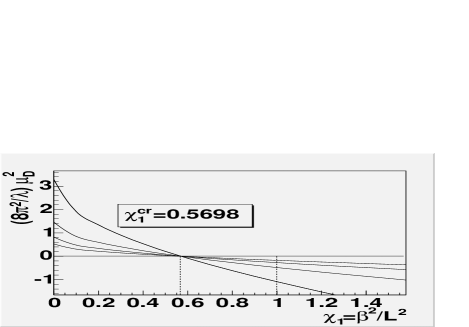
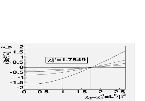
Figure 2: $(8\pi^{2}/\lambda)\mu_{D}^{2}$ versus $\chi_{1}$ (top) and $(8\pi^{2}/\lambda)\mu_{D}^{2}$ versus $\chi_{2}\equiv\chi_{1}^{-1}$ (bottom). The natural system $\hbar=c=k=1$ is used. For each curve on the top picture $\beta$ is fixed while $L$ evolves and, otherwise, for the bottom picture.

One can see the critical point $\chi_{1}^{cr}=0.5698$ at which $\mu^{2}_{D}$ changes the sign, i.e., there occurs the phase transition from the normal to the spontaneously broken phase. It is of importance that the phase transition can occur either because of changing the temperature at fixed $L$ (bottom picture) or because of the gap size $L$ changing at fixed temperature (top picture). The asymptotes of $\mu^{2}_{D}$ as $\chi_{1}\rightarrow 0$ ($L\rightarrow\infty$ while $\beta$ is fixed) and as $\chi_{2}\rightarrow 0$ ($\beta\rightarrow\infty$ while $L$ is fixed) are presented by the left edges of the top and bottom pictures, respectively, and are in agreement with Eqs. (10), (11). The results for the symmetric point $\beta=L$, i.e. $\chi_{1}=\chi_{2}=1$, are in agreement with the exactly calculated 16 sum $\sum^{\prime}\nolimits_{n,m}(-1)^{n}[n^{2}+m^{2}]^{-1}=(-1/2)\pi\ln 2$.

Let us also stress the essential advantage of the just considered dynamical mechanism of the spontaneous symmetry breaking (restoration). In our case, there are no problems with the perturbative calculation of the critical point as it occurs at investigation of the spontaneously broken symmetry restoration at critical temperature 3 , since we do not introduce into the Lagrangian the imaginary mass term by hand from the very beginning, that leads 17 to the complex value for the critical point.

It is obvious that in the case of the massless scalar electrodynamics with the Dirichlet BC on the gap plates, the evolution pictures are analogous to the presented by Fig. 2 ones with the same critical point. The only difference is in the asymptotes. Namely, $\mu^{2}_{D}\to\lambda T^{2}/18$ as $\chi_{1}\to 0$ ($L\to\infty$ while $T$ is fixed) and $\mu^{2}_{D}$ tends to the zero temperature result (15) as $\chi_{2}\to 0$ ($\beta\to\infty$ while $L$ is fixed). So, because of the gap size decreasing at fixed temperature at $\chi_{1}^{cr}=0.5698$, there occurs the phase transition: the massless scalar electrodynamics with the Dirichlet BC satisfied by the scalar fields on the gap boundaries transforms to the Higgs model with the spontaneous symmetry violation. As a result, at $\chi_{1}>\chi_{1}^{cr}$, after the realization of the standard Higgs mechanism, one leaves with the only massive scalar meson interacting with the massive vector boson.

Thus one can say that the boundary with the respective BC (Dirichlet here) and the temperature compete with each other: while the temperature always aspires to restore the broken symmetry, the boundary tends to violate it. This competition gives rise to the new type of phase transition: the decreasing in the characteristic size of the quantization region (the gap size here) and the increasing in the temperature tend to transport the system into the spontaneously broken or into the normal phase. The system evolves with a combined parameter reflecting the change in the temperature and in the size simultaneously. As a result, at the critical value of this parameter there occurs the phase transition from the normal to the spontaneously broken phase. In particular, the usual massless scalar electrodynamics transforms to the Higgs model. The later, as it is well known, is the key model supporting the foundations of main directions in the modern physics based on the spontaneous symmetry breaking and the Higgs mechanism. In particular, these are superconductivity theory 18 which is just the nonrelativistic variant of the Abelian Higgs model (see, for example, 19 and references therein) in the condense matter physics, and the Weinberg-Salam theory of the electroweak interactions in the high energy physics. So, one can hope that the presented here dynamical phenomena caused by the boundary influence can lead to some new physical predictions in these important branches of the modern physics.

In conclusion, let us stress that the present paper is, certainly, only one of the first steps in the investigation of the boundary induced dynamical phenomena. To be sure that the discussed in the paper just a possibility of the dynamical Higgs mechanism and of the respective phase transition is indeed realizable in reality, one should answer the still open questions. These are the such problems as the calculation of the mass term with the softened BC and the subsequent investigation of the mass term behavior away from the central domain, where one ought to study a nontrivial momentum dependence of the mass term and to perform the higher order analysis of the vertex functions; investigation of the respective dynamical phenomena within the strong coupling limit (lattice calculations); research on the influence of the nontrivial BC (like the Casimir ones) imposed on the gauge field, etc. This is, certainly, only a sketch of the main problems which require a detailed investigation in the future.