Lab/UFR-HEP0401/GNPHE/0404
Algebraic Geometry Realization
of Quantum Hall Soliton

Abstract

Using Iqbal-Netzike-Vafa dictionary giving the correspondence between the H₂ homology of del Pezzo surfaces and p-branes, we develop a new way to approach system of brane bounds in M-theory on $\mathbb{S}^{1}$. We first review the structure of ten dimensional quantum Hall soliton (QHS) from the view of M-theory on $\mathbb{S}^{1}$. Then, we show how the D0 dissolution in D2-brane is realized in M-theory language and derive the p-brane constraint eqs used to define appropriately QHS. Finally, we build an algebraic geometry realization of the QHS in type IIA superstring and show how to get its type IIB dual. Others aspects are also discussed.

Keywords: Branes Physics, Algebraic Geometry, Homology of Curves in Del Pezzo surfaces, Quantum Hall Solitons.

1 Introduction

Few years ago, it has been conjectured in [1], see also [2], that a specific assembly of a system of $KD0$, $D2$ and $N$ $D6$ branes and $N$ fundamental $F1$ strings, stretching between $D2$ and $D6$, has a low energy dynamics similar to the fundamental state of fractional quantum Hall (FQH) systems. There, the boundary states of the F1 strings ending on the D2 brane are interpreted as the FQH particles moving in the D2 brane world volume. The external strong magnetic field $B$ is represented by a large number of $D0$ branes dissolved in D2 and the dynamics of these particles is modeled by a non commutative Chern-Simons (NCCS) $U(1)$ gauge field theory [3]. Soon after this proposal, several constructions were considered pushing forward this analogy [4]-[12]. Susskind et al idea was also extended to quantum Hall solitons that are not of Laughlin type [13], in particular the quantum Hall solitons modeling Haldane hierarchy and multilayer systems as proposed in [14].

On other hand, it has been observed recently by Iqbal-Neitzke-Vafa (INV) [15] that there is remarkable correspondence between p-branes in M-theory on torii and holomorphic curves in del Pezzo surfaces. A dictionary characterizing this correspondence was given. The result of this work was particularly focused on the study of a mysterious duality in the toroidal compactification of M-theory, for other applications see also [16, 17]. But here we will use differently the INV link between del Pezzos and M-theory by developing a new method to approach brane systems. The originality of our construction rests on the fact that INV correspondence can be also used to study geometric aspects of brane physics using the power of algebraic geometry and homology. Among our results, we quote the derivation of new representations of p-brane systems using the H₂ homology of algebraic curves in del Pezzo surfaces.

To fix the idea on the way we will be doing things, we focus, in a first step, on a special system of branes and show how new representations can be built. The system we will be dealing with here concerns mainly the usual quantum Hall soliton (QHS) we have introduced in the beginning of this introduction. But in the discussion section, we will also draw the lines of other constructions, in particular the way QHS is realized in type IIB superstring on $\mathbb{S}^{1}$ as well as higher dimensional extensions.

The principal aim of this work is then to use results on ten dimensional QHS, the INV correspondence as well as string theory and mathematical results to develop new realizations of quantum Hall solitons using algebraic geometry curves in del Pezzo surfaces. For simplicity, we will give here the main lines of the method on Susskind et al QHS. A detailed analysis and applications dealing with other types of brane systems will be given in [18].

The presentation of this paper is as follows. In section 2, we describe briefly the Quantum Hall Soliton in type IIA superstring. We first review the structure of the ten dimensional QHS as formulated in literature and then give its representation in the language of the eleven dimensional M-theory on $\mathbb{S}^{1}$. This change from type IIA to M-theory allows us to reach the two remarkable points: (i) give a geometric realization of the standard idea of dissolution D0 branes in D2 and (ii) derive the appropriate geometric constraint eqs that define QHS. In section 3, we review the homology of del Pezzo surfaces as it is one of the basic tools in construction and in section 4 we describe the INV correspondence. In section 5 we first identify the constraint eqs for QHS using the H₂ homology of del Pezzos. Then we develop a realization of the Hall soliton using intersecting classes of complex curves in del Pezzos. In section 6, we give our conclusion and make a discussion.

2 Quantum Hall Solitons

One the remarkable observation of Susskind and collaborators in the derivation of the Quantum Hall Soliton is that the usual $\left(1+2\right)$ dimensional condensed matter Fractional Quantum Hall (FQH) phase has a striking similarity with a specific p-brane configuration in type IIA superstring theory. Following [1, 2], see also [19], there is a one to one correspondence between the 3d FQH systems of condensed matter physics and the low energy dynamics of brane bounds involving D0, D2 and D6-branes of the ten dimensional uncompactified type IIA superstring. There is also F1 strings stretching between D2 and D6 branes, F1 ends on D2 have an interpretation in terms of FQH particles ( Hall electrons). Let us comment briefly this configuration to which we shall refer here after as type IIA stringy representation of quantum Hall soliton. Denoting the usual IIA string (bosonic) coordinate field variables $X^{\mu}\left(\tau,\sigma\right)$ by the following equivalent and appropriate ones

$$\{t(\tau),\qquad\varrho(\tau,\sigma),\qquad\vartheta(\tau,\sigma),\qquad\varphi(\tau,\sigma),\qquad\{y^{i}(\tau,\sigma)\}_{4\leq i\leq 9;}\},$$ (2.1)

where $\tau$ and $\sigma$ are the usual string world sheet variables, the above mentioned p-brane bound system, called also Quantum Hall Soliton (QHS), is built as follows, see figure 1 for illustration:

2.1 Brane Configuration

If forgetting about edge excitations which may be modeled by NS5 branes, the simplest structure of QHS is parameterized in terms of the above ten dimensional string coordinates as follows:

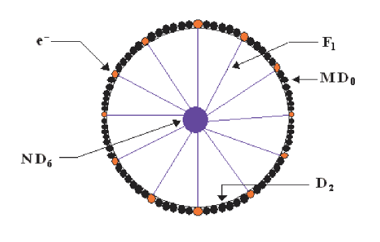
Figure 1: This figure represents the type IIA stringy representation of a fractional Quantum Hall Soliton.

(a) One two space dimensional spherical D2 brane, it plays role of the world volume in FQH systems of condensed matter physics and is parameterized by the spherical coordinates,

$$\{t,\qquad\varrho=R;\qquad 0\leq\vartheta\leq\pi;\qquad 0\leq\varphi\leq 2\pi;\qquad\mathbf{0_{6}}\}.$$ (2.2)

At fixed time, this D2-brane is embedded in $R^{3}\sim R^{+}\times S^{2}$ and for large values of the radius, D2 may be thought locally of as $R^{1,2}$ which is also interpreted as the space time of the three dimensional Chern Simons gauge theory.
(b) $N$ coincident flat six dimensional space D6 branes located at the origine of D2 and parameterized collectively by the $y^{i}$ internal Euclidean coordinates as,

$$\{t,\qquad\mathbf{{0_{3}},\qquad}\left(y^{4}\mathbf{,}...,y^{9}\right)\mathbf{\}.}$$ (2.3)

It can be thought of as an external source of charge density $J^{0}\propto N\delta^{3}(x)$ at the origin $(x^{1},x^{2},x^{3})=(0,0,0)$ of the spherical D2 brane.
(c) $N$ fundamental strings F1 stretching between D2 and D6 branes and parameterized by

$$\{t,\qquad 0\leq\varrho\leq R,\qquad\mathbf{{0_{2}},\qquad{0_{6}}\}}.$$ (2.4)

The F1 string ends on the D2 brane are associated to the electrons of the 3-dimensional condensed matter FQH fluids.
(d) $K$ D0-branes dissolved into the D2 brane; They define the flux quanta associated to the external magnetic field $B$ of FQH systems. Recall also that D0 and D6 are electric-magnetic dual.

2.2 Methods

Since the original work linking fractional quantum Hall fluids and NC Chern-Simons gauge theory [3], several methods have developed to deal with such kind of systems [5, 9]-[20]. Matrix model approach à la Polychronakos [21] is one these methods which has been getting a particular interest in literature. In this matrix model formulation, the FQH particles in the Laughlin state are described by two $N\times N$ hermitian matrices $X_{ij}^{1}(t)$ and $X_{ij}^{2}(t)$ ( in our coordinate choice $X_{ij}^{1}(t)\sim R\sin\vartheta_{ij}(t)\cos\varphi_{ij}(t)$ and $X^{2}(t)\sim R\sin\vartheta_{ij}(t)\sin\varphi_{ij}(t)$). For large radius R, the two sphere can be locally approximated by a flat patch of the $\mathbb{R}^{2}$ plane and so one can neglect, in a leading approximation, the curvature effect. In the infinite limit of $N$ and $M$ (strong external magnetic field), the one dimensional matrix fields $X_{ij}^{1}(t)$ and $X^{2}(t)$ are mapped to the usual (2+1) fields, a behaviour which is nicely given by Susskind map,

$$X^{i}(t,y)=y^{i}+\theta\varepsilon^{ij}A_{j}(t,y)$$ (2.5)

as discussed in [3, 10]. In this relation, one recognizes the $\left(1+2\right)$ Chern Simons gauge field $A_{j}(t,y)$ and the non commutativity parameter $\theta$ induced by the presence of external $B$.

In our present work, we will use a complete different approach to deal with the QHS. This method is based on algebraic geometry of del Pezzo surfaces and too particularly on their H₂ homology. In our way of doing, one may naturally define all physical quantities one encounters in type IIA stringy representation of QHS and condensed matter FQH fluids. For present presentation however and in the purpose of illustration of the technique, we will simplify the construction. We skip non necessary details and essentially focus on the path towards the algebraic geometry realization of QHS.

To proceed, let us say some words on our strategy towards the algebraic geometry realization of QHS. This will be done in four principal steps: (i) In step one, we reformulate the type IIA stringy representation of QHS as a constrained system of p-branes. Here we show that the appropriate way to do it is in fact from the view of M-theory on $\mathbb{S}^{1}$. In this case, we give a geometric realization of the idea of dissolution of D0 branes in D2 and show that QHS particles, namely electrons and flux quanta, can be treated in a quite similar manner. This step permits us to identify the appropriate geometric constraint eqs that define QHS. (ii) In step two, we review the INV correspondence and describe how p-branes are represented in algebraic geometry of del Pezzo surfaces. We take this opportunity to draw the main lines of a method of representing homology classes in the del Pezzo surface $\mathbb{B}_{1}$ by using F1 strings and D2 branes. This method uses triangulation property of surfaces and is also motivated from formal similarities with Feynman rules in quantum $\Phi^{3}$ theory. (iii) In step three, we reformulate the structure of the stringy QHS into the language of homology of del Pezzo surfaces. We first give the translation of constraint eqs in terms of H₂ homology of $\mathbb{B}_{1}$, then we study necessary conditions for their solutions. (iv) In last step, we develop a class of solutions of the homological constraint eqs giving an algebraic geometry realization of QHS.

We begin by noting that p-branes involved in the above QHS may, roughly speaking, be thought of as sets of points in p+1 dimensions. As far as brane links are concerned, we clearly see that intersections between the QHS branes may be naively defined as set intersections as follows:

$$D2\cap F1=1;\qquad D2\cap D6=0;\qquad D6\cap F1=1.$$ (2.6)

For the case of N fundamental strings, the first equation of above relations extends as $D2\cap\left(NF1\right)=N$ and so on. In ten dimensional type IIA stringy representation, these relations are natural identities that characterize the QHS and so they should be fulfilled in any other representation of QHS including the algebraic geometry one we are after. However to have a consistent description, we still need informations about the K D0 branes of the QHS and which have no reference in eq(2.6). This brings us to our first comment regarding this special property, which to our knowledge have not been sufficiently explored in literature. The idea of D0 dissolution in D2 is in fact strongly related with type IIA representation of QHS requiring that the total space-time dimension of the soliton should be equal to ten. However in eleven dimension M-theory on $\mathbb{S}^{1}$, we have an extra (compact) dimension which allows us to engineer in a nice geometric way the D0 branes in perfect agreement with INV correspondence. The key idea of our representation is summarized as follows: The D0 branes ( flux quanta) dissolved in D2 are treated in M-theory on $\mathbb{S}^{1}$ on equal footing as the electrons in the sense that they will be also viewed as ends of F1’ strings, but this time, stretching between D2 and K D0 branes, see figure1b for illustration.

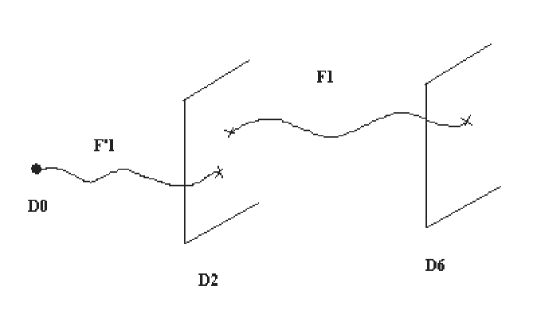
Figure 2: This figure represents the type IIA stringy representation of a fractional Quantum Hall Soliton.  The ends of F’1 strings on D2 are the D0 branes appearing in the Susskind el al QHS. They are in one to one with the KD0s associated with the eleventh ( compact) dimension.

From this representation, one clearly see that the total space time dimension of the QHS is as in M-theory on $\mathbb{S}^{1}$. One also see that D0 particles in QHS are associated with the compact direction $\mathbb{S}^{1}$ and moreover has much to do with the homological class of curve E_M in del Pezzo surface $\mathbb{B}_{1}$ considered in [15]. As such we have, in addition to eq(2.6), the following constraint eqs of QHS formulated in the language of M-theory on circle $\mathbb{S}^{1}$,

$$F^{\prime}1\cap D2 = 1,\qquad F^{\prime}1\cap D6=0$$

$$D0\cap F^{\prime}1 = 1,\qquad F^{\prime}1\cap F1=0$$ (2.7)

$$D0\cap D2 = 0,\qquad D0\cap D6=0,$$

where, leaving a part the brane dimension and their charge, there is a quite similar analogy between the role of D0 and D6 branes. With this reformulation of QHS in M-theory on $\mathbb{S}^{1}$ and to which we shall continue to refer to it as type IIA stringy representation, we end step one and are now in position to go ahead by following the drawn path. In the second step, we describe briefly some useful tools on the H₂ homology of del Pezzo surfaces and the INV correspondence between p-branes and complex curves.

3 Del Pezzo Surfaces

In this section, we focus on two basic aspects. First we give some useful tools on del Pezzo surfaces $\mathbb{B}_{k}$, $k=1,2,...,$ and too particularly on the H₂ homology of their class of curves. Then we consider the main lines of the toric representation of $\mathbb{B}_{1}$ as this will be also relevant for later analysis.

3.1 General on $\mathbb{B}_{k}$

Del Pezzo surfaces $\mathbb{B}_{k}$ are complex dimension two compact manifolds that are obtained by blowing up to eight points ($k\leq 8$) in complex projective space $\mathbb{P}^{2}$ [22, 23]. These $\mathbb{B}_{k}$ complex surfaces are simply laced manifolds and their homology $H_{2}\left(\mathbb{B}_{k},Z\right)$ is generated by the line class $H$ of $\mathbb{P}^{2}$ and the exceptional curves $E_{i}$ generating the $k$ blow ups of $\mathbb{P}^{2}$. The use of this line’s homology turns out to be very helpful in present study. It offers a poweful tool to study holomorphic curves in del Pezzos and has the advantage of giving a quite complete characterization of analytic curves without need to specify the explicit form of complex algebraic geometry equations.

Recall that on a compact algebraic and projective variety X, a generic divisor $\mathcal{D}=$ $\sum_{i}n_{i}\mathcal{D}_{i}$ is a finite formal linear combination of complex co-dimension one analytic subvarieties $\mathcal{D}_{i}$. An instructive illustration of this construction is given by the special case of a holomorphic function $F=F\left(x_{1},x_{2},...\right)$ on X,

$$F=\mathop{\displaystyle\prod}\limits_{j=1}^{s}F_{j}^{n_{j}}$$ (3.1)

with $F_{j}=F_{j}\left(x_{1},x_{2},...\right)$ being the irreducible components of F, they are holomorphic polynomials. Here the above $\mathcal{D}_{j}$s are the prime divisors associated with the zeros of $F_{j}$. The divisor $\mathcal{D}$, which is called principal, reads as $\left(F\right)=\sum_{j}n_{j}\left(F_{j}\right)$ with $n_{j}$ positive integers. The support of the divisor is the variety V$\left(F\right)=\mathcal{D}_{1}\cup\mathcal{D}_{2}\cup...\cup\mathcal{D}_{s}$. Similar relations are also valid for meromorphic functions with zeros and poles. Now, we turn to del Pezzo surfaces and their homology.

In a given del Pezzo surface $\mathbb{B}_{k}$, each $E_{i}$ is associated with a $\mathbb{P}^{1}$ holomorphic curve and the class system $\left\{H,E_{i}\right\}$ satisfies the following pairing,

$$H^{2}=1;\qquad H.E_{i}=0;\qquad E_{i}.E_{j}=-\delta_{ij};\qquad i,j=1,...,k.$$ (3.2)

In terms of these basic classes of curves, one defines all the tools we need for the present study. First, note that generic class of holomorphic curves in $\mathbb{B}_{k}$ are given by linear combinations type,

$$C_{a}=n_{a}H-\sum_{i=1}^{k}m_{ai}E_{i},$$ (3.3)

with $n_{a}$ and $m_{a}$ some integers. These classes of curves are characterized by two basic parameters: (a) The self-intersection number $C_{a}^{2}$, which by help of eq(3.2) is given by,

$$C_{a}^{2}=n_{a}^{2}-\sum_{i=1}^{k}m_{ai}^{2},$$ (3.4)

and (b) the degree $d_{C_{a}}$ which, as we shall see, is linked to the space-time dimension of the p-branes. Since the $C_{a}^{2}$ and the degree play a crucial role in the algebraic geometry realization of QHS we are considering in this paper, it is interesting to note that among the above classes of curves, there is a particular class of curves with a special property. This concerns the canonical class $\Omega_{k}$ of the $\mathbb{B}_{k}$ surface which is given by minus the first Chern class $c_{1}\left(\mathbb{B}_{k}\right)$ of the tangent bundle. It reads as,

$$\Omega_{k}=-\left(3H-\sum_{i=1}^{k}E_{i}\right),$$ (3.5)

and has a self intersection number $\Omega_{k}^{2}=9-k$ whose positivity requires $k\leq 9$. Obviously $k=0$ corresponds just to the case where we have no blow up; i.e the $\mathbb{P}^{2}$ complex surface. With the above relation, we are now in position to define the degree $d_{C}$ of a given curve class $C=nH-\sum_{i=1}^{k}m_{i}E_{i}$ in $\mathbb{B}_{k}$. It is the intersection number between the class $C$ with the anticanonical class $\left(-\Omega_{k}\right)$,

$$d_{C}=-C.\Omega_{k}=3n-\sum_{i=1}^{k}m_{i}.$$ (3.6)

Positivity of this integer puts a constraint equation on the allowed values of the $n$ and  $m_{i}$ integers which should be like $\sum_{i=1}^{k}m_{i}\leq 3n$. Note that there is a relation between the self intersection number $C^{2}$ of the classes of holomorphic curves and their degrees $d_{C}$. This relation, which is known as the adjunction formula, is given by

$$C^{2}=2g-2+d_{C},$$ (3.7)

it allows to define the genus $g$ of the curve class $C$ as $g=\left(2+n\left(n-3\right)-\sum_{i=1}^{k}m_{i}\left(m_{i}-1\right)\right)/2$ where we have also used the expansion $C=nH-\sum_{i=1}^{k}m_{i}E_{i}$. Fixing the genus $g$ to given positive number puts then a second constraint equation on $n$ and $m_{i}$ integers. For the interesting example of rational curves with $g=0$, we have then $C^{2}=d_{C}-2$ or equivalently

$$\sum_{i=1}^{k}m_{i}\left(m_{i}-1\right)=2+n\left(n-3\right).$$ (3.8)

For $k=1$, this relation reduces to $m\left(m-1\right)=2+n\left(n-3\right)$, its leading solutions $n=1,m=0$ and $n=0,m=-1$ give just the classes $H$ and $E$ respectively. Typical solutions for this constraint eq are given by the generic class $C_{n,n-1}=nH-\left(n-1\right)E$ which is more convenient to rewrite it as follows,

$$C_{n,n-1}=H+\left(n-1\right)\left(H-E\right)$$ (3.9)

In this case the degree of these rational curves in $\mathbb{B}_{1}$ is equal to $d_{C}=2n+1$, it deals then with p-branes in type IIA strings. However along with the above solution, there is also configurations with even degree. These solutions concerns NS branes given by the classes $C_{n,2-n}=C=nH-\left(2-n\right)E$ with $n=1,2$ and wrapped p-branes in type IIB representation. The second issue will be discussed later on.

3.2 Toric representation of $\mathbb{B}_{1}$

We need this toric representation to draw pictures for realizations of QHS in terms of classes of curves in $\mathbb{B}_{1}$. To that purpose recall first that toric representation is a tricky graphic representation that concerns complex manifolds [24, 25]. The latters can be usually imagined as given by a real base $\mathcal{B}$ with toric fibers on it. The simplest examples toric manifolds are naturally the complex projective spaces $\mathbb{P}^{n}$ where the real dimension n bases $\mathcal{B}_{n}$ are given by the usual n-simplex and fibers are n dimensional torii $\mathbb{T}^{n}$. Therefore in toric representation $\mathbb{P}^{1}$ is an interval of a straight line with a $\mathbb{S}^{1}$ circle on top and shrinking at the boundaries. Similarly $\mathbb{P}^{2}$ is a triangle with three vertices capturing toric singularities. The blow up of one of these three toric singularities of $\mathbb{P}^{2}$ is just $\mathbb{B}_{1}$ and is given by a rectangle with four vertices but only two toric singularities. The corresponding toric pictures of these three kinds of toric varieties are shown on figures 2.

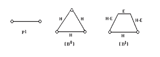
Figure 3: Three toric diagrams: (3a) Diagram of $\mathbb{P}^{1}$ with two $\mathbb{S}^{1}$ singularities on borders of the intervalle. (3b) Toric graph of $\mathbb{P}^{2}$ with three $\mathbb{T}^{2}$ toric singularities at the vertices and (3c) toric diagram of $\mathbb{B}_{1}$ with two toric singularities and a blown one.

In the $H_{2}$ homology of del Pezzo surfaces where line classes in $\mathbb{B}_{1}$ are of two types, the H standard hyperline and the E exceptional one, we have a nice description of these figures. Figures 2b and 2c are respectively given by the following canonical lines of $\mathbb{P}^{2}$ and $\mathbb{B}_{1}$,

$$-3H;\qquad-\left(3H-E\right)=-\left[H+2\left(H-E\right)+E\right].$$ (3.10)

Naively, these canonical classes may be thought as representing the boundaries of these complex surfaces, the triangle for $\mathbb{P}^{2}$ and rectangle for $\mathbb{B}_{1}$. Viewed in that way, these boundary lines are genus one classes having degrees $d_{-3H}=9$ and $d_{-3H+E}=8$ respectively, see eq(3.7). Moreover, the three edges of $\mathbb{P}^{2}$ (resp four for the case of $\mathbb{B}_{1}$) correspond just to the number of replication ( multiplicity) of the class H ( resp H and E for $\mathbb{B}_{1}$) of the basis of the $H_{2}\left(\mathbb{B}_{k},\mathbb{Z}\right)$ homology. In other words the three ( resp four) edges for the toric graph of $\mathbb{P}^{2}$ (resp $\mathbb{B}_{1}$) correspond to the splitting the multiplicity $-3H$ as $-H-H-H$. The same is also valid for the three ( four) vertices of the triangle ( rectangular), they correspond to the intersection points of the classes of curves.

Along with these figures, one may also draw the pictures associated with the rational curve classes of eq(3.9) inside the complex surfaces. Let us give some illustrating examples which will be used later on.

Graphs of the classes $H$ and $E$ in $\mathbb{B}_{1}$.

The hyperline class H has a self intersection one ($H^{2}=1$) and a degree $d_{H}=3$ giving the number of point on the boundary of $\mathbb{B}_{1}$. It looks like a three point Feynman diagram with three external legs and a three point vertex,

Figure 4: The graph of the class H in $\mathbb{B}_{1}$, it looks like the Latin letter Y. But as the 3-vertex can be everywhere $\mathbb{B}_{1}$, it can have different representation. In what follows, we will use the block representation given on right.

The unique self intersection point we have here belongs to the interior of the $\mathbb{B}_{1}$ surface and may be interpreted as a signature of the H class in $\mathbb{B}_{1}$, it is the 3-vertex of the triangulation of the surface. For the exceptional curve E, one may be interested to do the same as H. However this is not possible in H homological representation since E has a negative self interaction ($E^{2}=-1$). This means  that E cannot be drawn inside of the rectangle. This is why we will avoid this behaviour by changing the orthogonal basis $\left\{H,E\right\}$ of the $H_{2}\left(\mathbb{B}_{1},\mathbb{Z}\right)$ homology into the following equivalent one

$$H,\qquad H-E$$ (3.11)

where the previous difficulty $E^{2}=-1$ is now solved as $\left(H-E\right)^{2}=0$. The class of $H-E$ is a line in $\mathbb{B}_{1}$ with its two ends on the boundary. Note that contrary to the old basis $\left\{H,E\right\}$ which involves D0 and D2 branes, the new one implies instead F1 strings and D2 branes. Note in passing that $\mathbb{B}_{1}$ may be also defined using the following basis

$$l_{i}.l_{j}=1-\delta_{ij},\qquad i,j=1,2.$$ (3.12)

In this basis, the canonical class reads as $-2l_{1}-2l_{2}$ and genus zero curves of degree $2n+2$ are given by $C_{n,1}=nl_{1}+l_{2}$ or $C_{1,n}=l_{1}+nl_{2}$. They will be used later on when we consider type IIB stringy representation of QHS.

Graph of the class $H-E$ in $\mathbb{B}_{1}$

In the new basis eq(3.11) and thinking about the canonical class $\Omega_{-3H+E}$ of $\mathbb{B}_{1}$ as $-H-2\left(H-E\right)-E$, the class $H-E$ inside of $\mathbb{B}_{1}$is given by a line stretching between the basic H and E classes of $\Omega_{-3H+E}$. This goes in the same manner as do the two boundary ( external) lines $2\left(H-E\right)$ of the ” line frontier” class $\Omega_{-3H+E}$.

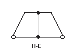
Figure 5: The internal line crossing the surface of rectangle defines the class $H-E$.  It may be viewed as a string stretching between two boundary points on $\mathbb{B}_{1}.$

The $H-E$ class has no self intersection ( no vertex).

Graph of the class $2H$ in $\mathbb{B}_{1}$

This is a genus zero class and has a degree equal to 6 and four self interaction points, its picture is immediately obtained by summing the graphs of two classes as $2H=H+H$. By superposition, we get in a first step the figure 3c1,

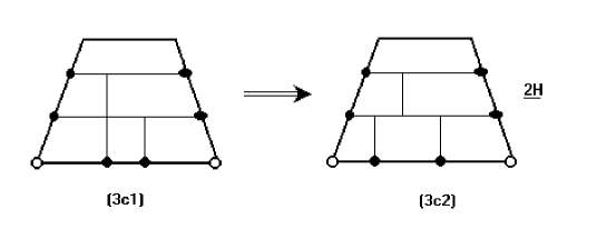
Figure 6: Graph representing the class $2H=H+H$. The diagrams on left and right describe respectively the class 2H before and after triangulation. In type IIA string language, this corresponds to NS5.

which involves two kinds of internal vertices, a three vertex and a four one. However splitting the four vertex into two 3-vertices using the the following triangulation rule,

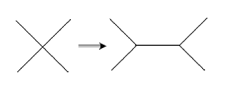
Figure 7: These figures show the triangulation of four vertex A into two three vertices A1 and A2.

we get figure on right with the appropriate number of internal three vertices. This property, which is general, is also valid for any sum of class of curves.

Graph of the class $2H-E$ in $\mathbb{B}_{1}$

Thinking about $2H-E$ as $H+\left(H-E\right)$ and following the same lines as before, it is not difficult to show that the figure representing this class of curve inside of $\mathbb{B}_{1}$ is given by.

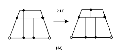
Figure 8: Building block of the homology class 2H-E. It represents a D4 brane in type IIA stringy description.

Here also we recognize the five external legs and the three self intersection points.

Graph of the class $3H-2E$ in $\mathbb{B}_{1}$

Repeating the same process, we get for this class of curve, thought of as the superposition of the following three basic curves $H+\left(H-E\right)+\left(H-E\right)$, the graph of figure 3e

Figure 9: Building block of the complex curve 3H-2E where one recognizes the five self intersection points. It represents a D6 branes in type IIA stringy description.

Such procedure is general and applies for all classes of the H₂ homology of del Pezzos. Details will be given in [18]

4 Branes and holomorphic curves

Following [15], there is a remarkable correspondence between del Pezzo surfaces $\mathbb{B}_{k}$ and M-theory on $\mathbb{T}^{k}$. Generally speaking an element $\omega$ of the real cohomology of del Pezzos associates the basic classes $\left(H,E_{1},...,E_{k}\right)$ of the surface $\mathbb{B}_{k}$ with the point $\left(l_{p},R_{1},...,R_{k}\right)$ in the moduli space of M-theory on $\mathbb{T}^{k}$. In practice, this means that $\omega$ is a kind of generalized Kahler acting as,

$$\omega\left(H\right)=-3\ln l_{p};\qquad\omega\left(E_{i}\right)=-\ln\left(2\pi R_{i}\right),$$ (4.1)

where $l_{p}$ is the Planck scale and where $R_{i}$s are the torus radii. Eq(4.1) is in fact a special one, it happens that INV correspondence is more general than given in eq(4.1). We have also the following correspondences: (a) Global diffeomorphisms preserving the canonical class $\Omega_{k}$ of the del Pezzo surfaces corresponds precisely to U duality group of M-theory on $\mathbb{T}^{k}$. (b) Rational curves (real two spheres) $C$ with volume V${}_{C}=\omega\left(C\right)$ and degree $d_{C}=\left(p+1\right)$ are in one to one with $\frac{1}{2}$ BPS p-brane states with tension $T_{p}=$2$\pi\exp V_{C}$. (c) Two classes of rational curves $C_{1}$ and $C_{2}$ related as $C_{1}+C_{2}=-\Omega_{k}$ corresponds just to the usual electric-magnetic duality linking Dp₁ and Dp₂ with $p_{1}+p_{2}=6$.

Therefore p-branes of ten dimensional IIA superstring can be realized as H${}_{2}\left(\mathbb{B}_{k},\mathbb{Z}\right)$ homology classes of holomorphic rational curves in $\mathbb{B}_{k}$. Of particular interest for our present study is the realization of p-branes in terms of H${}_{2}\left(\mathbb{B}_{1},\mathbb{Z}\right)$ classes. More precisely, given a generic $\mathbb{B}_{1}$ rational curve $C_{n,m}=nH-mE$ with a positive degree $3n-m$ and integers $n$ and $m$ constrained as $m\left(m-1\right)=2+n\left(n-3\right)$, we can work out all p-branes of type IIA superstring with space dimension $p$ equal to $3n-m-1$. The result is reported on the following table

BranesD0F1D2D4NS5D6D8,fragments BranesD0F1D2D4NS5D6D8\begin{tabular}[]{|l|l|l|l|l|l|l|l|}\hline\cr Classes&C${}_{0}$=E&C${}_{1}$=H-E&C${}_{2}$=H&C${}_{4}$=2H-E&C${}_{5}$=2H&C${}_{6}$=3H-2E&C${}_{8}$=4H-3E\\ \hline\cr Branes&D0&F1&D2&D4&NS5&D6&D8\\ \hline\cr\end{tabular}\ ,

ClassesC₀=EC₁=H-EC₂=HC₄=2H-EC₅=2HC₆=3H-2EC₈=4H-3EClassesC₀=EC₁=H-EC₂=HC₄=2H-EC₅=2HC₆=3H-2EC₈=4H-3E (4.2)

where now on the sub-index carried by the C_ps refers to the real space dimension of the p-branes. From this correspondence, one sees that previous figures we have drawn give indeed an algebraic geometry realization of p-branes in terms of classes of holomorphic rational curves in $\mathbb{B}_{1}$. With these tools in mind, we are now ready to consider the main topic of this paper.

5 Realization of QHS

To build a QHS representation using homology cycles of $\mathbb{B}_{1}$, we start by recalling that form the type IIA string representation of QHS we have the following first result,

$$\begin{tabular}[]{|l|l|l|l|l|l|}\hline\cr p-Branes&$D0$&$F^{\prime}1$&$D2$&$F1$&$D6$\\ \hline\cr Their realization in terms of Classes&$C_{0}$&$C_{1}^{\prime}$&$C_{2}$&$C_{1}$&$C_{6}$\\ \hline\cr\end{tabular}\ ,$$ (5.1)

It gives the p-branes involved in QHS and their realization in terms of classes of holomorphic curves in del Pezzo $\mathbb{B}_{1}$. Here $C_{1}^{\prime}$ refers to the class associated with fundamental strings stretching between D0 and D2 and $C_{1}$ to those F1 strings stretching between D2 and D6.

The next thing is to note that the problem of building algebraic geometry realizations of QHS reduces then to the finding of explicit forms of these $C_{p}$ class of curves in terms of the $H$ and $H-E$ fundamental classes,

$$C_{p}=C_{p}\left(H,E\right).$$ (5.2)

To do so, we first have to derive the appropriate constraint eqs that should be obeyed by these $C_{p}$s, then solve them. We will see that a solution of the form eq(5.2) that satisfy the QHS constraint eqs is not possible, one needs much more ingredients which we describe at proper time.

5.1 Constraint eqs and solution

By identifying the notion of set intersection in real geometry with the usual intersection of classes in H₂ homology of $\mathbb{B}_{1}$, the constraint relations (2.6-2.7) of type IIA string representation of QHS translate in H${}_{2}\left(\mathbb{B}_{1},\mathbb{Z}\right)$ homology language as follows:

$$C_{0}.C_{2} = 0;\qquad C_{0}.C_{6}=0;\qquad C_{2}.C_{6}=0,$$

$$C_{0}.C_{1}^{\prime} = 1;\qquad C_{1}^{\prime}.C_{2}=1;\qquad C_{1}^{\prime}.C_{6}=0,$$

$$C_{2}.C_{1} = 1;\qquad C_{2}.C_{6}=0;\qquad C_{1}.C_{6}=1,$$ (5.3)

$$C_{0}.C_{1} = 0;\qquad C_{1}^{\prime}.C_{1}=0;\qquad C_{2}.C_{1}=1$$

At first sight, solving these constraint eqs for rational curves in del Pezzo $\mathbb{B}_{1}$ seems a simple matter. However, this is no so trivial. While the intersection of classes type $C_{2}.C_{1}=1$ or $C_{6}.C_{1}=1$ do cause no problem, the situation is not so obvious for the constraint eqs $C_{2}.C_{6}=0$, $C_{0}.C_{2}=0$ and $C_{0}.C_{6}=0$. The point is that there are no class of curves in $\mathbb{B}_{1}$ with such a feature. This is easily seen by directly computing  the corresponding products. For instance the product between $C_{2}=H$ and $C_{6}=3H-2E$, using eqs(3.2), gives,

$$C_{2}.C_{6}=3,$$ (5.4)

and same thing for the other relations, which are not as required by the structure of the QHS we are after. A way to over pass this difficulty is to think about the three classes $C_{0}$, $C_{2}$ and $C_{6}$ as belonging to three independent del Pezzo surfaces $\mathbb{B}_{1}^{\left(-1\right)},$ $\mathbb{B}_{1}^{\left(0\right)}$ and $\mathbb{B}_{1}^{\left(1\right)}$ as,

$$C_{0}^{\left(-1\right)}=E_{-1};\qquad C_{2}^{\left(0\right)}=H_{0};\qquad C_{6}^{\left(1\right)}=3H_{1}-2E_{1},$$ (5.5)

where in addition to eq(3.2), we also have $H_{0}.H_{\pm 1}=H_{0}.E_{\pm 1}=H_{\pm 1}.E_{0}=0$, see also figure 6. In this case, it is not difficult to check that the intersection products $C_{0}^{\left(-1\right)}.C_{2}^{\left(0\right)}$, $C_{0}^{\left(-\right)}.C_{6}^{\left(1\right)}$ and $C_{2}^{\left(0\right)}.C_{6}^{\left(1\right)}$ are identically zero. The introduction of the $\mathbb{B}_{1}^{\left(-1\right)},$ $\mathbb{B}_{1}^{\left(0\right)}$ and $\mathbb{B}_{1}^{\left(1\right)}$ surfaces is the price one should pay for getting solutions of QHS constraint eqs. As such one can think about these three surfaces as three special sub-manifolds of the blown up of three different $\mathbb{P}^{2}$s embedded in $\mathbb{P}^{8}$. The two extra dimensions in $\mathbb{P}^{8}$ deal with the curves $C_{1}^{\prime}$ and $C_{1}$ associated with F’1 and F1 strings stretching between the two pairs $\mathbb{B}_{1}^{\left(-1\right)}-\mathbb{B}_{1}^{\left(0\right)}$ and $\mathbb{B}_{1}^{\left(0\right)}-\mathbb{B}_{1}^{\left(1\right)}$ respectively. Therefore a simple solution for the constraint eqs (5.3) read as follows

$$C_{0}^{\left(-1-1\right)} = E_{-1},$$

$$C_{1}^{\left(-10\right)} = H_{-1}-E_{0};\qquad C_{1}^{\left(0-1\right)}=H_{0}-E_{-1},$$

$$C_{2}^{\left(00\right)} = H_{0},$$ (5.6)

$$C_{1}^{\left(01\right)} = H_{0}-E_{1};\qquad C_{1}^{\left(10\right)}=H_{1}-E_{0},$$

$$C_{6}^{\left(11\right)} = 3H_{1}-2E_{1},$$

where the upper index $\left(ij\right)$ refers to the $\left(i,j\right)$ pair of the involved del Pezzos. The couple $\left(00\right)$ (resp($\left(\pm 1\pm 1\right)$) means that we are dealing with classes of curves in $\mathbb{B}_{1}^{\left(0\right)}$ ( resp $\mathbb{B}_{1}^{\left(\pm 1\right)}$) and $\left(0\pm 1\right)$ or $\left(\pm 10\right)$ with rational curves stretching between $\mathbb{B}_{1}^{\left(0\right)}$ and $\mathbb{B}_{1}^{\left(\pm 1\right)}$. Naturally, the full solution for stretched F1 strings is given by the sum $C_{1}^{\left(0\pm 1\right)}+C_{1}^{\left(\pm 10\right)}$ which is equal to $\left(H_{0}-E_{\pm 1}\right)+\left(H_{\pm 1}-E_{0}\right)$.

In the above solution (5.6) of the constraint eqs for QHS we have considered one D6 brane and one D0 brane and same for the F1 string stretching between D0-D2 and D2-D6. These p-branes are represented by $H_{2}\left(\mathbb{B}_{1}^{\left(0,\pm 1\right)},\mathbb{Z}\right)$ classes describing rational holomorphic curves. In what follows, we derive the general solution of eqs(5.3) involving ND6-branes and KD0-ones, N and K are arbitrary positive integers.

5.2 Quantum Hall Soliton

The algebraic geometry realization of QHS built in terms of a system of intersecting curves is as follows, see figure 6 for illustration

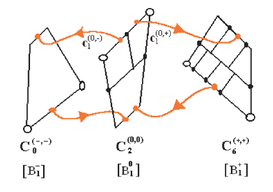
Figure 10: In this figure, we give a configuration of the homological representation of the QHS involving classes C₀, C₂ and C₆ respectively associated with one D0, one D2 and one D 6 branes. We also represent the curves C₁ illustrating strings stretching between the branes.

(1) A simple rational curve class $C_{2}^{\left(00\right)}=H_{0}$ belonging to a basic of del Pezzo copy denoted as $\mathbb{B}_{1}^{\left(0\right)}$ and generated by $H_{0}$ and $E_{0}$ basic classes with same properties as above. This class of curve is associated with the D2 brane in type IIA stringy representation.
(2) A class of curve with a multiplicity $N$ given by the class $C_{6}^{\prime}=N\left(3H_{1}-2E_{1}\right)$. This is a non zero genus class ($2g=N\left(5N-7\right)+2$) that corresponds to the N coincident D6 branes in the IIA string representation of QHS. To see from where comes this result, it is interesting to recall that in the case where the N D6 branes are not coincident, the previous degenerate class split into N simple classes of curves $C_{6}^{\left(ii\right)}$ given by

$$C_{6}^{\left(ii\right)}=3H_{i}-2E_{i},\qquad i=1,...,N.$$ (5.7)

Each one of these N $C_{6}^{\left(ii\right)}$s belongs to one of the N del Pezzo copies $\mathbb{B}_{1}^{\left(i\right)}$. The latters have basis $\left\{H_{i},E_{i}\right\}$ with same properties as before but orthogonal to the $\left\{H_{j},E_{j}\right\}$ whenever $i\neq j$. This means that in H₂ homology, the N D6 branes involve N copies of del Pezzo surfaces $\mathbb{B}_{1}^{\left(1\right)},...,\mathbb{B}_{1}^{\left(N\right)}$ and so requires a larger embedding projective space. To have an idea on the dimension of this space, note that, in addition to F1 string loops $C_{1}^{\left(ii\right)}=\left(H_{i}-E_{i}\right)$ emanating and ending on the same $C_{6}^{\left(ii\right)}$ copy, we have moreover other F1 strings stretching between the D6 branes. In H₂ homology, this correspond to curves $C_{1}^{\left(ij\right)}$ and $C_{1}^{\left(ji\right)}$ stretching between $\mathbb{B}_{1}^{\left(i\right)}$ and $\mathbb{B}_{1}^{\left(j\right)}$. The explicit expression of these classes is given by

$$C_{1}^{\left(ij\right)} = \left(H_{i}-E_{j}\right);\qquad C_{6}^{\left(ii\right)}.C_{1}^{\left(ij\right)}=1;\qquad C_{1}^{\left(ij\right)}.C_{6}^{\left(jj\right)}=1$$

$$C_{1}^{\left(ji\right)} = \left(H_{j}-E_{i}\right),;\qquad C_{1}^{\left(ji\right)}.C_{6}^{\left(ii\right)}=1;\qquad C_{6}^{\left(jj\right)}.C_{1}^{\left(ji\right)}=1.$$ (5.8)

From these relations, one clearly see that the $C_{1}^{\left(ij\right)}$ and $C_{1}^{\left(ji\right)}$ classes are stretching between the $C_{6}^{\left(ii\right)}$ and $C_{6}^{\left(jj\right)}$. Since these $C_{1}^{\left(ij\right)}$ and $C_{1}^{\left(ji\right)}$ classes require at least one complex dimension, the embedding projective space should be at least $\mathbb{P}^{3N-1}$. In type IIA stringy representation, this situation describes the case where the gauge symmetry is $U\left(1\right)^{N}$. For the case of $U\left(N\right)$ gauge symmetry, the D6 branes should be coincident and so the corresponding curve classes $C_{6}^{\left(ii\right)}$ have to be degenerate curves in $\mathbb{B}_{1}$. This corresponds to,

$$NC_{6}=C_{6}^{\prime}=N\left(3H_{1}-2E_{1}\right),$$ (5.9)

where $H_{1}$ and $E_{1}$stand for the basic classes of the del Pezzo surface $\mathbb{B}_{1}$ where live the degenerate $NC_{6}$.
(3) $N$ holomorphic curves $C_{1}^{\left(0i\right)}+C_{1}^{\left(i0\right)}$ solved as $\left(H_{0}-E_{i}\right)+\left(H_{i}-E_{0}\right)$ and stretching between $C_{2}^{\left(00\right)}$ and $C_{6}^{\left(ii\right)}$. For the case of N coincident D6 branes eq(5.9), the N classes $C_{1}^{\left(0i\right)}+C_{1}^{\left(i0\right)}$ fuse and give

$$C_{1}^{\left(01\right)} = NH_{0}-E_{1}$$

$$C_{1}^{\left(10\right)} = H_{1}-NE_{0},$$ (5.10)

where obviously the F1 strings stretching between $C_{2}^{\left(00\right)}$ and the $NC_{6}^{\left(ii\right)}$ are collectively described by the sum $\left(NH_{0}-E_{1}\right)+\left(H_{1}-NE_{0}\right)$. From these solutions, it not difficult to check that the constraint eqs (LABEL:cst1) are exactly fulfilled.
(4) Finally for the $K$ D0-branes describing the quantum flux, the construction is quite similar to what we have done for the case of coincident D6 branes. The homology class describing the K D0 branes is $C_{0}^{\left(-1-1\right)}=kE_{-1}$ and the F’1 strings stretching between the kD0 and D2 realized as $C_{0}^{\left(-1-1\right)}$ and $C_{2}^{\left(00\right)}$ are given by

$$C_{1}^{\left(-10\right)}=\left(kH_{0}-E_{-1}\right)+\left(H_{-1}-kE_{0}\right),$$ (5.11)

They quantum fluxes are naturally given by the ends of the F’1 strings on $C_{2}^{\left(00\right)}$ and so are associated with the intersection number $C_{1}^{\left(-10\right)}.C_{2}^{\left(00\right)}=k$ in agreement with the constraint eqs.

6 Conclusion and Discussion

Using a recent result linking p-branes and holomorphic curves in del Pezzo surfaces, we have developed a new way to deal with brane bounds of M-theory on $\mathbb{S}^{1}$. To illustrate our idea in an explicit manner, we have considered the usual type IIA stringy representation of the quantum Hall soliton (QHS) and derived its realization by using the H₂ homology of del Pezzo surfaces. In our representation, QHS is described by a system of intersecting classes of holomorphic curves as given by eqs(5.7-5.11), see also figure 6.

The idea developed here can be used to derive new solutions for QHS but also for studding general branes systems. The development of these issues seems to us important, it offers an other way to approach p-brane bounds and uses the powerful tools of homology groups and algebraic geometry that may allow to open new horizons. In particular, one may derive new representations of higher dimensional quantum Hall solitons involving two D4-branes and F1 strings stretching between them in the same spirit as in [26, 27, 28]. One may also consider QHS using p-branes of type IIB superstring that are dual to the previous type IIA ones. In the algebraic geometry of QHS we have been considering, this configuration can be obtained without major difficulty. It consists of the system D3/S¹, D7/S¹, F1, D1 and D1/S¹ and satisfy similar constraint eqs to relations(5.3). The correspondence between the two representations is as follows,

Curves in 𝔹1HH−EE2H−E3H−2EType IIBD3/S1F1, D1F1/S1, D1/S1D5/S1D7/S1Curves in 𝔹2l1+l2−el1,l2l1−e,l2−e2l1+l2−e3l1+l2−e,fragments fragmentsCurves in B1𝐻fragmentsHE𝐸fragments2HEfragments3H2EType IIBfragmentsD3/S1F1, D1fragmentsF1/S1, D1/S1fragmentsD5/S1fragmentsD7/S1fragmentsCurves in B2fragmentsl1l2efragmentsl1,l2fragmentsl1e,l2efragments2l1l2efragments3l1l2e\begin{tabular}[]{|l|l|l|l|l|l|}\hline\cr Type IIA&D2&F1&D0&D4&D6\\ \hline\cr Curves in $\mathbb{B}_{1}$&$H$&$H-E$&$E$&$2H-E$&$3H-2E$\\ \hline\cr Type IIB&D3/S${}^{1}$&F1, D1&F1/S${}^{1}$, D1/S${}^{1}$&D5/S${}^{1}$&D7/S${}^{1}$\\ \hline\cr Curves in $\mathbb{B}_{2}$&$l_{1}+l_{2}-e$&$l_{1},l_{2}$&$l_{1}-e,l_{2}-e$&$2l_{1}+l_{2}-e$&$3l_{1}+l_{2}-e$\\ \hline\cr\end{tabular},

Type IIAD2F1D0D4D6Type IIAD2F1D0D4D6 (6.1)

where $l_{i}.l_{j}=1-\delta_{ij},$ $l_{i}.e=0$ and $e.e=-1$ . To algebraic geometry engineer the corresponding QHS dual to the type IIA one, all one has to do is, instead of the surface $\mathbb{B}_{1}$ generated by $l_{1}$ and $l_{2}$, one considers rather the del Pezzo surface $\mathbb{B}_{2}$, see figure 7

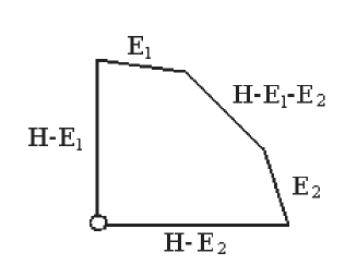
Figure 11: This graph represents the toric diagram of the del Pezzo surface $\mathbb{B}_{2}$.

The extra blow up described by the exceptional class $e$ deals with the brane wrapping cycle $\mathbb{S}^{1}$. The solution to the constraint eqs may be obtained without difficulty by using the mapping

$$e=H-E_{1}-E_{2};\qquad l_{1}=H-E_{1};\qquad l_{2}=H-E_{2}$$ (6.2)

Applying the rules we have used in elaborating the type IIA stringy realization of quantum Hall soliton, we can draw here also the graphs of the F1, D1 strings and the wrapped D-branes D3/S¹ and D7/S¹ involved in the type IIB stringy representation of QHS. We have,

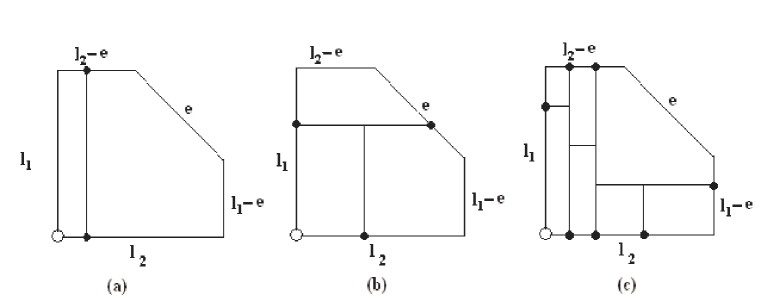
Figure 12: These are three graphs of curves in the del Pezzo surface $B_{2}$, they are involved in the type IIB stringy representation of QHS. These classes are associated with branes in type IIB string on $S^{1}$. Figure 12a gives a representation of F1 string. Figure 12b represents a wraped D3 brane on a circle and figure 12c describes a wrapped D7 brane on a circle.

Using these graphs, one can also build the QHS diagram similar to that given by figure 10. Details on this issue as well as other aspects dealing with the derivation of new solitons including higher dimensional QHS with a configuration type D4-F1-D4-D0 will be presented elsewhere.

Acknowledgement 1

Ait Ben Haddou thanks Department of Mathematics, Faculty of Meknes and M. Zaoui for support. Abounasr, El Rhalami and Saidi thank A Belhaj, L. El Fassi, A Jellal and E M Sahraoui for earlier collaborations on these issues. This research work is supported by Protars III D12/25 CNRT (Rabat).

References

- [1] B.A.Bernevig, J. Brodie, L. Susskind, N. Toumbas, How Bob Laughlin Tamed the Giant Graviton from Taub-NUT space, JHEP 0102:003,2001 and hep-th/0010105.
- [2] L. Susskind, Lectures delivred at stias, Stellenbosch 2001, South Africa,
- [3] L. Susskind, The Quantum Hall Fluid and Non-Commutative Chern Simons Theory, (2001) hep-th/0101029.
- [4] Simeon Hellerman, Leonard Susskind, hep-th/0107200.
- [5] John H. Brodie, D-branes in Massive IIA and Solitons in Chern-Simons Theory, hep-th/0012068, JHEP 0111 (2001) 014.
- [6] O. Bergman, J. Brodie, Y. Okawa, The Stringy Quantum Hall Fluid, JHEP 0111 (2001) 019, hep-th/0107178.
- [7] Steven S. Gubser, Mukund Rangamani, D-Brane Dynamics and the Qunatum Hall Effect. JHEP 0105:041,2001; hep-th/0012155
- [8] Simeon Hellerman, Leonard Susskind; Realizing the Quantum Hall System in String Theory,hep-th/0107200
- [9] Michal Fabinger, Higher-Dimensional Quantum Hall Effect in String Theory, JHEP 0205 (2002) 037, hep-th/0201016.
- [10] S. Hellerman and M. Van Raamsdonk, JHEP 0110 (2001) 039, hep-th/0103179.
- [11] A. Jellal, E.H. Saidi and H.B. Geyer, A Matrix Model for Fractional Quantum Hall States, hep-th/0204248.
- [12] A. Jellal, E.H. Saidi, H.B. Geyer and R.A. Römer, J. Phys. Soc. Japan 72 (2003) A127, hep-th/0303143. A. Jellal, E.H. Saidi, H.B. Geyer, R.A. Roemer, J.Phys.Soc.Jap. 72 (2003) A127.
- [13] A. El Rhalami, E.M. Sahraoui and E.H. Saidi, JHEP 05 (2002) 004, hep-th/0108096;
- [14] A. El Rhalami, and E.H. Saidi, JHEP 10 (2002) 39, hep-th/0208144,
- [15] Amer Iqbal, Andrew Neitzke, Cumrun Vafa, A Mysterious Duality, Adv.Theor.Math.Phys. 5 (2002) 769-808, hep-th/0111068.
- [16] Pierre Henry-Labordere, Bernard Julia, Louis Paulot, Borcherds symmetries in M-theory, JHEP 0204 (2002) 049, hep-th/0203070. Real Borcherds Superalgebras and M-theory, JHEP 0304 (2003) 060, hep-th/0212346.
- [17] Jeffrey Brown, Ori J. Ganor, Craig Helfgott, M-theory and E10: Billiards, Branes, and Imaginary Roots, hep-th/0401053.
- [18] Work in preparation
- [19] H.B.Geyer(Ed):Field Theory, Topology and Condensed matter Physics,Proceedings of the Ninth Chris Engelbrecht Summer School in theoretical Physics. Held at:Storms River Mouth, Tsitsikamma National Parkc, South africa, 17-28 January 1994.Springer 1995. (see) A.Zee,Quatum Hall Fluid.
- [20] El Hassan Saidi, NC Geometry and Fractional Branes, Class.Quant.Grav. 20 (2003) 4447-4472, hep-th/0311245.
- [21] A.P. Polychronakos, JHEP 0104 (2001) 011, hep-th/0103013.
- [22] M. Demazure, surface de del Pezzo, lectures notes in mathematics 777 springer 1980,William Fulton, algebraic curves, Mathematics lecture Note series, Benjamin / Cummings Publishing compagny
- [23] P. Griffits and Harris, Principles of algebraic geometry, J. Wiley & Sons, New York 1994, Y.I Manin, cubic forms; Algebra, geometry, arithmetics. North Holland publishing cC, Amsterdam 1986.
- [24] N.C. Leung, C. Vafa, Branes and Toric Geometry, Adv.Theor.Math.Phys. 2 (1998) 91-118, hep-th/9711013.
- [25] A. Belhaj, E.H Saidi, Toric Geometry, Enhanced non Simply laced Gauge Symmetries in Superstrings and F-theory Compactifications, hep-th/0012131, Mod.Phys.Lett. A15 (2000) 1767-1780, hep-th/0007143, Class.Quant.Grav. 18 (2001) 57-82.
- [26] Shou-Cheng Zhang, Jiangping Hu, A Four Dimensional Generalization of the Quantum Hall Effect, Science 294 (2001) 823, cond-mat/0110572.
- [27] D. Karabali and B. Sakita, Phys. Rev. B64 (2001) 245316, hep-th/0106016; Phys. Rev. B65 (2002) 075304, hep-th/0107168.
- [28] Ali Hafoud, Thèse de Doctorat Nationale, Département de Mathématique, Faculté des Sciences, Rabat, fall (2002)