Solving Witten’s SFT by Insertion of Operators on Projectors

Haitang Yang

Center for Theoretical Physics

Massachussetts Institute of Technology,

Cambridge, MA 02139, USA

E-mail: hyanga@mit.edu

Abstract

Following Okawa, we insert operators at the boundary of regulated star algebra projectors to construct the leading order tachyon vacuum solution of open string field theory. We also calculate the energy density of the solution and the ratio between the kinetic and the cubic terms. A universal relationship between these two quantities is found. We show that for any twist invariant projector, the energy density can account for at most $68.46\%$ of the D25-brane tension. The general results are then applied to regulated slivers and butterflies, and the next-to-leading order solution for regulated sliver states is constructed.

1 Introduction and Summary

The tachyon instability in open string theory comes from the expansion of the action around the perturbative vacuum. Sen conjectured that there is a nonperturbative vacuum where D25-branes decay and only closed string excitations exist [1, 2]. However, no analytic solution that represents the stable tachyon vacuum has been found so far. Level truncation is a powerful method to construct numerical solutions [2]-[7]. Very impressive results have been obtained in [7, 5], where the D25-brane tension was reproduced at very high accuracy. Level truncation, however, can only give solutions satisfying the equation of motion when contracted with the solutions themselves, as opposed to an arbitrary state in the Fock space.

A new approach was developed by Okawa [22] who inserted operators at the middle point of the boundary of regulated butterfly states [23]-[26]. This approach has some similarities to level truncation. One inserts linear combinations of operators with the same mass dimension order by order. The solution, in the case of butterflies, is a series expanded with powers of $\sqrt{1-t}$, where $t$ is the regulation parameter and $t\to 1$ gives the exact butterflies. The solution obtained by this approach satisfies the equation of motion when contracted with arbitrary states in the Fock space. At the same time, finite results are obtained when calculating the energy density.

It is of interest to see if this approach can also be applied to other star algebra projectors. The butterfly state is just a special case of generalized butterfly states characterized by a parameter $\alpha$ [26], with $\alpha=1$ for butterfly sate. It is natural to ask if the results depend on the parameter $\alpha$ or not. Can we write down an analytical expression for the energy density obtained from solution based on a general star algebra projector?

We are only concerned with twist invariant projectors in this paper. For this kind of projectors, the middle point of the boundary can be defined to be the point which reaches the string middle point as the regulator is removed. All the projectors currently known have this property. A twist invariant projector $|P\rangle$ can be defined by:

$$\langle\phi|P\rangle=\langle f\circ\phi(0)\rangle_{\mathbb{H}_{z}},\hskip 14.22636ptz=f(\xi),$$ (1.1)

where $\mathbb{H}_{z}$ stands for the full upper half $z$ plane and $\langle\phi|$ is an arbitrary state in the Fock space, inserted at the puncture $\xi=0$ in the local coordinate patch. The ambiguity of $f(\xi)$ is removed, up to a scale, by requiring $f(0)=0$ and $f(1)=-f(-1)$. The definition of a regulated projector $|P_{t}\rangle$ is:

$$\langle\phi|P_{t}\rangle=\langle f_{t}\circ\phi(0)\rangle_{\mathbb{H}_{z}},\hskip 14.22636ptz=f_{t}(\xi),$$ (1.2)

on $z$ representation, where $t$ is the regulation parameter. $f_{t}(\xi)$ is required to satisfy the conditions:

$$f_{t}(0)=0,\hskip 14.22636ptf_{t}(1)=-f_{t}(-1),\hskip 14.22636pt\lim_{t\to 0}f_{t}(\xi)=f(\xi).$$ (1.3)

The operators will be inserted at the boundary midpoint of the regulated projectors. In the $z$ representation of twist invariant regulated projectors, this point is located at infinity, so it is convenient to map it to the origin. For this purpose, we introduce a new $\eta$ representation. $\eta$ is obtained as $\eta=I\circ z=-\frac{1}{z}$.

In order to calculate the leading order solution that represents the tachyon vacuum, besides the map $\eta=I\circ f_{t}(\xi)$, one also needs a map $\eta^{\prime}=I\circ\tilde{f}_{t}(\xi)$, where $\tilde{f}_{t}(\xi)$ defines the star product of two regulated projectors in $z$ representation:

$$\langle\phi|P_{t}*P_{t}\rangle=\langle\tilde{f}_{t}\circ\phi(0)\rangle_{\mathbb{H}_{z}},$$ (1.4)

with $\tilde{f}_{t}(0)=0$ and $\tilde{f}_{t}(1)=-\tilde{f}_{t}(-1)$. To simplify the calculations, we will scale $\tilde{f}_{t}(\xi)$ to have the limit $\tilde{f}_{t}(\xi)\to f(\xi)$ as $t\to 0$. Therefore, one can construct a map $\eta^{\prime}=g_{t}(\eta)$ with $g_{t}(0)>0$ which maps two copies of the surface associated with $|P_{t}\rangle$ to the glued surface associated with $|P_{t}*P_{t}\rangle$. $g_{t}(\eta)$ plays the role of star product and tells us where the boundary midpoints of the two surfaces associated with $|P_{t}\rangle$’s are located on the surface associated with $|P_{t}*P_{t}\rangle$. We find the leading order solution is:

$$\psi^{(0)}=-a_{t}|P_{t}(c)\rangle,$$ (1.5)

where $a_{t}=\frac{g_{t}^{\prime}(0)^{2}}{2g_{t}(0)}>0$ and $|P_{t}(c)\rangle$ denotes a general twist invariant regulated projector with a $c$ ghost insertion at the boundary middle point.

Inner products of projectors are encountered when one calculates the energy density. We will assume the availability of a map $h(\eta)$, which maps a single regulated projector in $\eta$ representation, after cutting the local coordinate patch and gluing the left half string with the right half string, to a unit disk. $h(\eta)$ is fixed by mapping the boundary midpoint to $1$ and string midpoint to the origin on the unit disk. We show that the ratio of the kinetic term to cubic interaction is:

$$R=\lim_{t\to 0}\frac{\langle\psi^{(0)}|Q_{B}|\psi^{(0)}\rangle}{\langle\psi^{(0)}|\psi^{(0)}*\psi^{(0)}\rangle}=-2^{4}\cdot 3^{-9/2}\lim_{t\to 0}\frac{b_{t}}{a_{t}},$$ (1.6)

where $b_{t}=-ih^{\prime}(0)>0$. Since both $a_{t}$ and $b_{t}$ are positive, $R$ is negative. Ideally, $R=-1$ from the equation of motion. The limit $\lim_{t\to 0}b_{t}/a_{t}$ is conformally invariant because the scale freedom of $a_{t}$ is cancelled by that of $b_{t}$. The ratio of the energy density at the solution and the D25-brane tension is:

$$\frac{\cal E}{T_{25}} = 2\pi^{2}\Big{[}\frac{1}{2}\langle\psi^{(0)}|Q_{B}|\psi^{(0)}\rangle+\frac{1}{3}\langle\psi^{(0)}|\psi^{(0)}*\psi^{(0)}\rangle\Big{]}$$ (1.7)

$$= 2\pi^{2}\lim_{t\to 0}\Big{[}-8\Big{(}\frac{a_{t}}{b_{t}}\Big{)}^{2}+3^{7/2}\Big{(}\frac{a_{t}}{b_{t}}\Big{)}^{3}\Big{]}.$$

A universal relationship between $R$ and ${\cal E}/T_{25}$ is found:

$$\frac{\cal E}{T_{25}}=-\frac{\pi^{2}}{3}\left(\frac{4}{3\sqrt{3}}\right)^{6}\frac{3R+2}{R^{3}}\simeq-0.6846\times\frac{3R+2}{R^{3}},$$ (1.8)

where $-0.6846$ is the familiar value of ${\cal E}/T_{25}$ at level zero obtained in [4]. The quantity ${\cal K}(R)\equiv\frac{3R+2}{R^{3}}$ reaches its maximum at the optimal value $R=-1$: ${\cal K}(-1)=1$. When applied to regulated butterflies, these equations reproduce the results of [22]. When applied to regulated slivers, namely wedge states, it gives:

$$R=-2\left(\frac{4}{3\sqrt{3}}\right)^{3}\simeq-0.9124,\hskip 14.22636pt\frac{\cal E}{T_{25}}=2\pi^{2}\,\frac{3^{7/2}-64}{8}\simeq-0.6645.$$ (1.9)

In the calculations, two maps $h(\eta)$ and $\tilde{f}_{t}(\xi)$ are needed. Generically, it is not difficult to calculate $h(\eta)$. However, obtaining $\tilde{f}_{t}(\xi)$ is challenging. For butterflies, this map [25] takes a rather complicated form. On the other hand, $\tilde{f}_{t}(\xi)$ for regulated slivers is very simple. Higher order calculations are much simplified if one starts from regulated slivers. Therefore, it is also of interest to calculate the next to leading order results based on slivers. We find that there is only one solution with:

$$R\simeq-0.9209,\hskip 14.22636pt\frac{\cal E}{T_{25}}=-0.81736.$$ (1.10)

The organization of this paper is as follows. In section 2, we construct the leading order solution for a general twist invariant regulated projector and calculate the energy density. We then apply the results to regulated sliver and butterfly states in section 3. Section 4 is devoted to the calculation of the next to leading order solution based on regulated slivers. In section 5, we give our conclusions.

2 The leading order solution for general star algebra projectors

The action of Witten’s cubic string field theory is [27]:

$$S[\Phi]=-\frac{1}{g^{2}}\left[\frac{1}{2}\langle\Phi|Q_{B}|\Phi\rangle+\frac{1}{3}\langle\Phi|\Phi*\Phi\rangle\right],$$ (2.1)

where $Q_{B}$ stands for the BRST operator and $g$ is the open string coupling constant. The equation of motion of this action takes the form:

$$Q_{B}|\Phi\rangle+|\Phi*\Phi\rangle=0.$$ (2.2)

A solution $|\psi\rangle$ of this theory should satisfy the equation of motion when contracted with an arbitrary state $|\phi\rangle$ in the Fock space:

$$\langle\phi|Q_{B}|\psi\rangle+\langle\phi|\psi*\psi\rangle=0,$$ (2.3)

and with the solution itself:

$$\langle\psi|Q_{B}|\psi\rangle+\langle\psi|\psi*\psi\rangle=0.$$ (2.4)

Furthermore, the energy density calculated from the solution is expected to cancel D25-brane tension [1],

$${\cal E}[\psi]=\frac{1}{g^{2}}\left[\frac{1}{2}\langle\psi|Q_{B}|\psi\rangle+\frac{1}{3}\langle\psi|\psi*\psi\rangle\right],\hskip 14.22636pt\frac{\cal E}{T_{25}}=-1,$$ (2.5)

with $T_{25}=\frac{1}{2\pi^{2}g^{2}}$, where we have assumed, without losing generality, that the brane has unit volume.

A general twist invariant star algebra projector $|P\rangle$ can be defined on the upper half $z$ plane representation by :

$$\langle\phi|P\rangle=\langle f\circ\phi(0)\rangle_{\mathbb{H}_{z}}.$$ (2.6)

$f(\xi)$ is fixed up to a scale by $f(0)=0$ and the twist invariant condition $f(1)=-f(-1)$. A regulated projector $|P_{t}\rangle$ is then defined by:

$$\langle\phi|P_{t}\rangle=\langle f_{t}\circ\phi(0)\rangle_{\mathbb{H}_{z}},$$ (2.7)

with the puncture located at $z=0$ and the middle point of the boundary lying at $z=\infty$. $f_{t}(1)=-f_{t}(-1)$ fixes $f_{t}(\xi)$ up to a scale. We can set this scale ambiguity as the same as that of $f(\xi)$. Therefore, we have

$$\lim_{t\to 0}f_{t}(\xi)=f(\xi),\hskip 14.22636pt\lim_{t\to 0}\langle\phi|P_{t}\rangle=\langle\phi|P\rangle=\langle I\circ f\circ\phi(0)\rangle_{\mathbb{H}_{z}}.$$ (2.8)

The map $f_{t}(\xi)$, or equivalently, the shape of the local coordinate patch on the upper half $z$ plane carries all the information of the regulated projector. Since we will insert the operators on the middle point of the boundary, the following $\eta=I(z)=-\frac{1}{z}$ representation is useful:

$$\langle\phi|P_{t}\rangle=\langle I\circ f_{t}\circ\phi(0)\rangle_{\mathbb{H}},$$ (2.9)

which maps the middle point of the boundary to $\eta=0$, as illustrated in figure (1). The star product of two projectors can be easily done in $\hat{z}$ representation. In this representation, the image of the local coordinate patch is the full strip $\Re(\hat{z})\leq\pi/4$, $\Im(\hat{z})\geq 0$ and the middle point of the string is mapped to $\hat{z}=i\infty$ under the map $\hat{z}=\arctan\xi$. One removes the local coordinate patch of the first projector, and glues the right half string of the first projector with the left half string of the second projector. Then we can map the glued surface in $\hat{z}$ representation to $\eta$ representation and obtain:

$$\langle\phi|P_{t}*P_{t}\rangle=\langle I\circ\tilde{f}_{t}\circ\phi(0)\rangle_{\mathbb{H}}.$$ (2.10)

In principle, $\tilde{f}_{t}(\xi)$ can be derived from $f_{t}(\xi)$, but this is a nontrivial task. So far, we only know $\tilde{f}_{t}(\xi)$ for sliver and butterfly states [23, 25]. The ambiguity of $\tilde{f}_{t}(\xi)$ is fixed up to a scale by $\tilde{f}_{t}(0)=0$ and $\tilde{f}_{t}(1)=-\tilde{f}_{t}(-1)$. In the $\eta$ representation, we denote:

$$\eta=I\circ f_{t}(\xi),\hskip 14.22636pt\eta^{\prime}=I\circ\tilde{f}_{t}(\xi).$$ (2.11)

From the construction of the star product of projectors mentioned above, there exists a map:

$$\eta^{\prime}=g_{t}(\eta)$$ (2.12)

which tells us where the inserted operators for each single projector are mapped on the glued $\eta^{\prime}$ plane. This map is a one to two map. $g_{t}(0)$ has two values with opposite signs which represent the locations of the two insertions on the glued $\eta^{\prime}$ surface. We will choose $g_{t}(0)>0$ without losing generality.

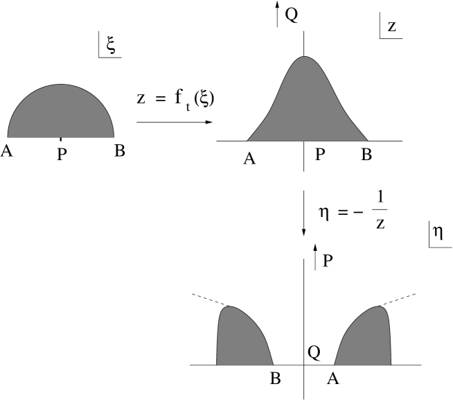
Figure 1: The canonical half disk on the $\xi$ plane is the local coordinate patch with $\xi(P)=0$ being the puncture. This half disk is mapped to some region around the origin on the upper half $z$ plane, with the middle point of the boundary $Q$ lying at infinity. On the $\eta=I(z)=-\frac{1}{z}$ representation, $Q$ lies at the origin and $P$ lies at infinity.

2.1 The leading order solution

At the first order, the $c$ ghost is inserted at the boundary midpoint of the regulated projector. We use the notation $|P_{t}(c)\rangle$ to denote this operator insertion. Therefore, on the $\eta$ representation,

$$\langle\phi|P_{t}(c)\rangle=\langle I\circ f_{t}\circ\phi(\xi=0)\,c(\eta=0)\rangle_{\mathbb{H}},$$ (2.13)

for an arbitrary state $|\phi\rangle$ in the Fock space. Since the BRST transformation of $c$ ghost is simply $Q_{B}\circ c=c\partial c$, the kinetic term in the action (2.1) gives:

$$\langle\phi|Q_{B}|P_{t}(c)\rangle = \langle I\circ f_{t}\circ\phi(0)\,c\partial c(0)\rangle_{\mathbb{H}}$$ (2.14)

$$= \langle I\circ f\circ\phi(0)\,c\partial c(0)\rangle_{\mathbb{H}}+{\cal O}(t),$$

where we have used the fact that one has the freedom to choose the regulation parameter $t$ to make $f_{t}(\xi)=f(\xi)+{\cal O}(t)$. For the cubic term, one has to glue two projectors, each of which has $c$ ghost inserted at $\eta=0$. Therefore, one has to transform $c(0)$ in each $\eta$ surface onto the glued $\eta^{\prime}$ surface,

$$\langle\phi|P_{t}(c)*P_{t}(c)\rangle=\frac{1}{g_{t}^{\prime}(0)^{2}}\langle I\circ\tilde{f}_{t}\circ\phi(0)c(-g_{t}(0))c(g_{t}(0))\rangle_{\mathbb{H}},$$ (2.15)

with $g_{t}(0)>0$. The order of the two operators $c(-g_{t}(0))$ and $c(g_{t}(0))$ is arranged to keep the orientation of the surface unchanged after mapping. For any projector, we have $\tilde{f}_{t}(\xi)=kf(\xi)+{\cal O}(t^{\alpha})$ with $\alpha>0$ and $k$ being the scale constant. If $\tilde{f}_{t}(\xi)$ is analytic with respect to $t$, $\alpha$ is some positive integer. Therefore, $g_{t}(0)\sim{\cal O}(t^{\beta})$ with $\beta>0$. Thus, both $c(-g_{t}(0))$ and $c(g_{t}(0))$ approach $c(0)$ as $t\to 0$. We need to evaluate the OPE of the two $c$ insertions.

$$\langle\phi|P_{t}(c)*P_{t}(c)\rangle=\frac{2g_{t}(0)}{k\,g_{t}^{\prime}(0)^{2}}\Big{(}\langle I\circ f\circ\phi(0)\,c\partial c(0)\rangle_{\mathbb{H}}\Big{)}+{\cal O}(t^{\alpha+\beta})+{\cal O}(t^{3\beta}).$$ (2.16)

Suppose on the $\eta$ representation, the leading order solution takes the form:

$$|\psi^{(0)}\rangle=-a_{t}|P_{t}(c)\rangle,$$ (2.17)

where $a_{t}$ is some constant. From the equation of motion $\langle\phi|Q_{B}|\psi\rangle+\langle\phi|\psi*\psi\rangle=0$, comparing equations (2.14) and (2.16), one can identify $a_{t}={kg_{t}^{\prime}(0)^{2}}/{2g_{t}(0)}$. It is straightforward to see that $a_{t}$ is scale invariant. Therefore, we simply choose $k=1$ in our paper and obtain:

$$a_{t}=\frac{g_{t}^{\prime}(0)^{2}}{2g_{t}(0)},$$ (2.18)

provided $\beta<1$ and $\beta<\alpha$ because the equation of motion based on this solution now reads:

$$\langle\phi|Q_{B}|\psi^{(0)}\rangle+\langle\phi|\psi^{(0)}*\psi^{(0)}\rangle={\cal O}(t^{1-\beta})+{\cal O}(t^{\alpha-\beta})+{\cal O}(t^{\beta}).$$ (2.19)

Since $g_{t}^{\prime}(0)$ must be real from the orientations of the surface before and after mapping, $a_{t}$ is positive. Therefore, the leading order solution in $\eta$ representation is:

$$|\psi^{(0)}\rangle=-\frac{g_{t}^{\prime}(0)^{2}}{2g_{t}(0)}|P_{t}(c)\rangle.$$ (2.20)

We see that as $t\to 0$, the coefficient $-\frac{g_{t}^{\prime}(0)^{2}}{2g_{t}(0)}$ becomes singular for any projector.

2.2 The energy density for the leading order solution

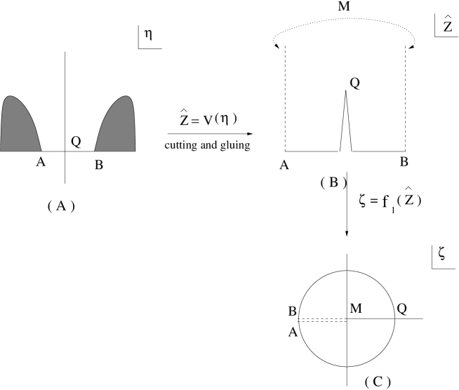
Figure 2: Figure (A) is a general twist invariant regulated projector in the $\eta$ representation. This projector is mapped to $\hat{z}$ representation by $\hat{z}=v(\eta)=\arctan\circ(I\circ f_{t})^{-1}(\eta)$. After cutting the local coordinate patch and identify the left half string $AM$ with the right half string $BM$, figure (B) is obtained. Then figure (B) is mapped to a unit circle in $\zeta$ plane by $f_{1}(\hat{z})$ in figure (C). $M$ is the string middle point, which lies at $i\infty$ in $\hat{z}$ representation and mapped to the origin in $\zeta$ plane. $Q$ is the boundary middle point, which is mapped to $\zeta=1$ on the unit disk.

In the last subsection, we obtained the leading order solution for general star algebra projectors. We want to use this solution to calculate the energy density. In the calculations, one encounters the inner products of regulated projectors. Therefore, we first map the regulated projector in $\eta$ representation to $\hat{z}$ representation. After gluing the projectors in $\hat{z}$ representation, one can map the resulted surface to a unit disk and then evaluate the expectation values.

Let’s first consider a single regulated projector on $\eta$ representation. The map from $\eta$ representation to $\hat{z}$ representation is:

$$\hat{z}=\arctan\circ(I\circ f_{t})^{-1}(\eta)\equiv v(\eta).$$ (2.21)

After cutting the local coordinate patch and identifying the right half string with the left half string, we next map this surface to a unit disk on the $\zeta$ plane with the middle point of boundary $Q$ mapped to $\zeta=1$ and the middle point of the string $M$ mapped to $\zeta=0$ by:

$$\zeta=f_{1}(\hat{z})=f_{1}\circ v(\eta)\equiv h(\eta),$$ (2.22)

as illustrated in figure (2). Since AM is glued with BM, $f_{1}(\hat{z})$ is periodic with respect to $\hat{z}$. Usually, it is not very hard to figure out $f_{1}(\hat{z})$ for a particular projector. For an instance, for the generalized butterfly states [26] parametrized by $0\leq\alpha\leq 2$, after cutting and gluing, one can translate and rescale the surface via $\frac{2\alpha}{2-\alpha}(\hat{z}-\pi/4)$ to obtain the same surface as a regulated butterfly state. The map for a regulated butterfly state from the $\hat{z}$ representation to the upper half plane is $f_{t}(\hat{z})=\frac{\tan\hat{z}}{\sqrt{1+t^{2}\tan^{2}\hat{z}}}$ with $t$ being the regulation parameter. Therefore, for the generalized butterfly states, we find:

$$f_{1}(\hat{z})=\frac{\sqrt{1+t^{\prime 2}\tan^{2}(\frac{2\alpha}{2-\alpha}(\hat{z}-\pi/4))}+i\sqrt{1-t^{\prime 2}}\tan(\frac{2\alpha}{2-\alpha}(\hat{z}-\pi/4))}{-\sqrt{1+t^{\prime 2}\tan^{2}(\frac{2\alpha}{2-\alpha}(\hat{z}-\pi/4))}+i\sqrt{1-t^{\prime 2}}\tan(\frac{2\alpha}{2-\alpha}(\hat{z}-\pi/4))},$$ (2.23)

with $t^{\prime}=\tanh(\frac{2\alpha}{2-\alpha}\tanh^{-1}t)$, where $t$ is the regulation parameter. We will simply assume this map is given for any twist invariant projector.

Figure 3: Mapping the inner product of two projectors in $\hat{z}$ representation to a unit disk in $\zeta$ plane.

Then the map from the inner product of two regulated projectors in the $\hat{z}$ representation to a unit disk in the $\zeta$ plane is $f_{1/2}(\hat{z})=\sqrt{f_{1}(\hat{z})}$, as illustrated in figure (3) . From the periodicity of $f_{1}(\hat{z})$, we can see that $f_{1}(Q_{1})=f_{1}(Q_{2})$ as well as $f_{1/2}(Q_{1})=-f_{1/2}(Q_{2})=1$, where $Q_{1}$ and $Q_{2}$ are the boundary middle points of the two regulated projectors. For the inner product of three regulated projectors, the map is $f_{1/3}(\hat{z})=f_{1}^{1/3}(\hat{z})$ with $f_{1}(Q_{1})=f_{1}(Q_{2})=f_{1}(Q_{3})$ as well as $f_{1/3}(Q_{1})=1$, $f_{1/3}(Q_{2})=\exp(i2\pi/3)$, $f_{1/3}(Q_{3})=\exp(i4\pi/3)$, with $Q_{1}$, $Q_{2}$ and $Q_{3}$ being the boundary middle points of the three regulated projectors. Therefore,

$$\langle P_{t}(c)|Q_{B}|P_{t}(c)\rangle = \frac{A^{2}}{f_{1/2}^{\prime}(\hat{z}(Q_{1}))f_{1/2}^{\prime}(\hat{z}(Q_{2}))}\langle c(1)c\partial c(-1)\rangle_{D}$$ (2.24)

$$= \frac{-4A^{2}}{f_{1/2}^{\prime}(\hat{z}(Q_{1}))f_{1/2}^{\prime}(\hat{z}(Q_{2}))},$$

with

$$A=-\frac{1}{v^{\prime}(\eta=0)}\frac{g_{t}^{\prime}(0)^{2}}{2g_{t}(0)}=-\frac{1}{[\arctan\circ(I\circ f_{t})^{-1}(\eta=0)]^{\prime}}\frac{g_{t}^{\prime}(0)^{2}}{2g_{t}(0)},$$ (2.25)

from equation (2.22). The cubic interaction is:

$$\langle P_{t}(c)|P_{t}(c)*P_{t}(c)\rangle=\frac{i3\sqrt{3}A^{3}}{f_{1/3}^{\prime}(Q_{1})f_{1/3}^{\prime}(Q_{2})f_{1/3}^{\prime}(Q_{3})}.$$ (2.26)

From the periodicity of $f_{1}(\hat{z})$, we have

$$f_{1/2}^{\prime}(Q_{1})f_{1/2}^{\prime}(Q_{2})=\frac{f_{1}^{\prime 2}(Q_{1})}{4f_{1/2}(Q_{1})f_{1/2}(Q_{2})}=-\frac{f_{1}^{\prime 2}(Q_{1})}{4},$$ (2.27)

for the kinetic term and

$$f_{1/3}^{\prime}(Q_{1})f_{1/3}^{\prime}(Q_{2})f_{1/3}^{\prime}(Q_{3})=\frac{f_{1}^{\prime 3}(Q_{1})}{27},$$ (2.28)

for the cubic interaction. It sometimes happens that $\frac{1}{[v(\eta=0)]^{\prime}}$, which appears in the expression of $A$ and $f_{1}^{\prime}(Q_{1})$, is singular for some projectors. Actually, this occurs for the butterflies. This is because $\psi^{(0)}$ is not well defined in $\hat{z}$ representation for some regulated projectors. However, the map $h(\eta)$ to a unit disk defined in (2.22) is well defined for any projector. Therefore, we write:

$$\lim_{t\to 0}\langle P_{t}(c)|Q_{B}|P_{t}(c)\rangle=\lim_{t\to 0}\frac{16}{h^{\prime}(\eta=0)^{2}}\Big{(}\frac{g_{t}^{\prime}(0)^{2}}{2g_{t}(0)}\Big{)}^{2},$$ (2.29)

$$\lim_{t\to 0}\langle P_{t}(c)|P_{t}(c)*P_{t}(c)\rangle=-\lim_{t\to 0}\frac{i3^{9/2}}{h^{\prime}(\eta=0)^{3}}\Big{(}\frac{g_{t}^{\prime}(0)^{2}}{2g_{t}(0)}\Big{)}^{3},$$ (2.30)

where we have set $t\to 0$ and only kept the leading order. Let us define:

$$b_{t}\equiv-ih^{\prime}(\eta=0).$$ (2.31)

One can justify $b_{t}$ is positive because $h^{\prime}(0)=i\times$ (a real number) by considering the orientations of the surface before and after mapping. Thus, the ratio between the kinetic term and the cubic interaction is:

$$R=\lim_{t\to 0}\frac{\langle\psi^{(0)}|Q_{B}|\psi^{(0)}\rangle}{\langle\psi^{(0)}|\psi^{(0)}*\psi^{(0)}\rangle}=-2^{4}\cdot 3^{-9/2}\lim_{t\to 0}\frac{b_{t}}{a_{t}},$$ (2.32)

which is always negative. The ratio of the energy density at this solution to D25-brane tension is:

$$\frac{\cal E}{T_{25}}=2\pi^{2}\lim_{t\to 0}\Big{[}-8\Big{(}\frac{a_{t}}{b_{t}}\Big{)}^{2}+3^{7/2}\Big{(}\frac{a_{t}}{b_{t}}\Big{)}^{3}\Big{]}.$$ (2.33)

One can see that both quantities only depend on one positive number: $\lim_{t\to 0}\frac{b_{t}}{a_{t}}$. A universal relationship between $R$ and ${\cal E}/T_{25}$ follows:

$$\frac{\cal E}{T_{25}}=-\frac{\pi^{2}}{3}\left(\frac{4}{3\sqrt{3}}\right)^{6}\frac{3R+2}{R^{3}}\simeq-0.684616\times\frac{3R+2}{R^{3}},$$ (2.34)

independent of the details of the projectors. The number $-0.6846$ is the famous one obtained in the first order level truncation calculations. The quantity $\frac{3R+2}{R^{3}}$ acquires its maximum at the ideal value $R=-1$. Therefore, we can conclude that for any twist invariant projector, at the leading order, the energy density can account for at most $68.4616\%$ of the D25-brane tension.

3 The leading order solution for regulated sliver and butterfly states.

In this section, we will apply the results obtained in last section to regulated sliver and butterfly states. The results for the regulated butterfly state are exactly the same as those obtained in [22]. We will verify the solution for the regulated sliver state by checking the equation of motion (2.4) and the ratio of energy density to D25-brane tension in (2.5), when contracted with itself.

3.1 Results for the regulated slivers

The regulated sliver state is a wedge state parametrized by $n$. As $n\to\infty$, one obtains the real sliver state $|\Xi\rangle$. For a single wedge state $|n\rangle$,

$$\langle\phi|n\rangle=\langle f\circ\phi(0)\rangle_{C_{n}}=\langle I\circ f_{n}\circ f\circ\phi(0)\rangle_{\mathbb{H}},$$

with $f(\xi)=\arctan\xi$ and $f_{n}(\hat{z})=\frac{n}{2}\tan\left(\frac{2}{n}\hat{z}\right)$ [29], where we have already mapped the middle point of the boundary to $\eta=0$ as required in equation (2.12). The surface $C_{n}$ is a cylinder with perimeter $\frac{n\pi}{2}$ on upper half plane, defining the wedge state $|n\rangle$ in $\hat{z}$ representation, as illustrated in figure (4).

Figure 4: A wedge state $|n\rangle$ is defined by the surface $C_{n}$ on $\hat{z}$ representation. After cutting the local coordinate patch and gluing left half string with right half string, one obtains $C_{n-1}$ surface on $\hat{z}$. $f_{1}(\hat{z})$ maps $C_{n-1}$ to a unit disk with that the image of $Q$ is $\zeta=1$ and the image of $M$ is $\zeta=0$.

For the star product of two wedge states:

$$\langle\phi|n*n\rangle=\langle f\circ\phi(0)\rangle_{C_{2n-1}}=\langle I\circ\tilde{f}_{n}\circ f\circ\phi(0)\rangle_{\mathbb{H}},$$

where $\tilde{f}_{n}(\hat{z})=f_{2n-1}(\hat{z})=\frac{2n-1}{2}\tan\left(\frac{2}{2n-1}\hat{z}\right)$. The map from a single wedge state to the glued one in $\eta$ representation is:

$$g_{n}(\eta)=\frac{2}{(2n-1)\tan\Big{[}\frac{n}{2n-1}\arctan\frac{2}{n\eta}\big{]}}.$$

Thus,

$$a_{n}=\frac{g_{n}^{\prime}(0)^{2}}{2g_{n}(0)}=\frac{n^{4}}{4(2n-1)^{3}\cos\frac{n\pi}{4n-2}\sin^{3}\frac{n\pi}{4n-2}}=\frac{n}{8}+{\cal O}(1).$$

From equation (2.20), in $\eta$ representation, the leading order solution is:

$$|\psi^{(0)}\rangle=-\frac{n}{8}|n(c)\rangle.$$ (3.1)

It is straightforward to calculate $v(\eta)$:

$$\hat{z}=v(\eta)=\arctan\circ(I\circ f_{n}\circ f)^{-1}(\eta)=-\frac{n}{2}\arctan\frac{2}{n\eta}.$$ (3.2)

For a wedge state $|n\rangle$ in the $\hat{z}$ representation with boundary midpoint at $\hat{z}(Q)=\frac{n\pi}{4}$ and string midpoint at $\hat{z}(M)=i\infty$, after cutting the local coordinate patch and gluing the left half string with the right half string, one obtains the surface $C_{n-1}$. Then, as introduced in equation (2.22),

$$f_{1}(\hat{z})=\exp\left(i\frac{4}{n-1}(\hat{z}-n\pi/4)\right),$$ (3.3)

maps this $C_{n-1}$ surface to a unit disk with the image of $\hat{z}(Q)$ being $\zeta=1$ and the image of $\hat{z}(M)$ being the origin $\zeta=0$, as illustrated in figure (4). This map can also be obtained readily from equation (2.23) by setting $\alpha=2/n$ as well as $t=0$. Therefore,

$$b_{n}=-ih^{\prime}(0)=-i(f_{1}\circ v(\eta=0))^{\prime}=\frac{n^{2}}{n-1}.$$ (3.4)

From equations (2.29) and (2.30), the leading order solution gives:

$$\lim_{n\to\infty}\langle\psi^{(0)}|Q_{B}|\psi^{(0)}\rangle=-\frac{1}{4},$$ (3.5)

$$\lim_{n\to\infty}\langle\psi^{(0)}|\psi^{(0)}*\psi^{(0)}\rangle=\left(\frac{3\sqrt{3}}{8}\right)^{3}.$$ (3.6)

The ratio of the kinetic term to the cubic interaction which is expected to be $-1$ from the equation of motion reads:

$$R=\lim_{n\to\infty}\frac{\langle\psi^{(0)}|Q_{B}|\psi^{(0)}\rangle}{\langle\psi^{(0)}|\psi^{(0)}*\psi^{(0)}\rangle}=-2\left(\frac{4}{3\sqrt{3}}\right)^{3}=-0.9124.$$ (3.7)

The ratio of the energy density to D25-brane tension is:

$$\lim_{n\to\infty}\frac{{\cal E}}{T_{25}}=2\pi^{2}\left(-\frac{1}{8}+\frac{3^{7/2}}{8^{3}}\right)=-0.6645.$$ (3.8)

Compared with the value $-0.6846$ obtained by level truncation at the first tachyon level, this ratio is rather close.

3.2 Solution of the regulated butterflies

A regulated butterfly state $|B_{t}\rangle$ characterized by a parameter $t\in[0,1)$ is defined by:

$$\langle\phi|B_{t}\rangle=\langle f_{t}(\xi)\circ\phi(0)\rangle_{\mathbb{H}_{z}},\hskip 14.22636ptf_{t}(\xi)=\frac{\xi}{\sqrt{1+t^{2}\xi^{2}}},$$ (3.9)

for an arbitrary state $|\phi\rangle$ in the Fock space. As $t\to 1$, one obtains the exact butterfly state $|B\rangle$. The solution based on regulated butterfly states was calculated in [22] by Okawa to the next to leading order. From equation (2.33) in [22], $g_{t}(0)=\beta$ and $g_{t}^{\prime}(0)=\sqrt{\frac{48}{(1-t^{4})(1-a^{2})(3+a^{2})}}\beta^{2}$ with $\beta=\frac{2}{9-a^{2}}\sqrt{(1-a^{2})(3+a^{2})}$ and $a=\sqrt{3}\tan\left(\frac{2}{3}\arctan t\right)$. Therefore,

$$a_{t}=\frac{g_{t}^{\prime}(0)^{2}}{2g_{t}(0)}=\frac{3^{1/4}}{4\sqrt{2}}\frac{1}{\sqrt{1-t}}+{\cal O}(\sqrt{1-t}).$$ (3.10)

Thus, the leading order solution in $\eta$ representation is:

$$|\psi^{(0)}\rangle=-\frac{3^{1/4}}{4\sqrt{2}}\frac{1}{\sqrt{1-t}}|B_{t}(c)\rangle,$$ (3.11)

exactly the same as equation (2.41) in [22]. Given $f_{t}(\xi)=\frac{\xi}{\sqrt{1+t^{2}\xi^{2}}}$, one obtains:

$$\hat{z}=v(\eta)=\arctan\circ(I\circ f_{t})^{-1}(\eta)=\frac{\pi}{2}+i\,\mbox{arctanh}\,\sqrt{t^{2}-\eta^{2}},$$ (3.12)

with the normalization that the boundary middle point is mapped to $\hat{z}=\frac{\pi}{2}+i\,\mbox{arctanh}\,t$. The surface obtained by cutting the local coordinate patch and gluing the left half string with the right half string of a regulated butterfly state in $\hat{z}$ representation is mapped to a unit disk on $\zeta$ plane by equation (2.23) with $\alpha=1$:

$$f_{1}(\hat{z})=\frac{\tan(2\hat{z}-\pi/2)-i\sqrt{1+q^{2}+q^{2}\tan^{2}(2\hat{z}-\pi/2)}}{\tan(2\hat{z}-\pi/2)+i\sqrt{1+q^{2}+q^{2}\tan^{2}(2\hat{z}-\pi/2)}},$$ (3.13)

with $q=\frac{2t}{1-t^{2}}$. The string midpoint is mapped to $\zeta(M)=0$ and the image of the boundary midpoint is located at $\zeta(Q)=1$. Therefore,

$$b_{t}=-ih^{\prime}(0)=-i(f_{1}\circ v(\eta=0))^{\prime}=4(1-t^{4})^{-1/2}.$$ (3.14)

From equations (2.29), (2.30), (2.32) and (2.33),

$$\lim_{t\to 1}\langle B_{t}(c)|Q_{B}|B_{t}(c)\rangle=-\frac{\sqrt{3}}{8},$$ (3.15)

$$\lim_{t\to 1}\langle B_{t}(c)|B_{t}(c)*B_{t}(c)\rangle=3^{21/4}2^{-21/2},$$ (3.16)

as well as

$$R = -2^{15/2}\cdot 3^{-19/4},$$

$$\frac{\cal E}{T_{25}} = 2\pi^{2}\left(-\frac{\sqrt{3}}{16}+3^{17/4}2^{-21/2}\right)+{\cal O}(1-t).$$ (3.17)

All the results agree with those obtained in [22].

4 Subleading solution for a regulated sliver state

In the last few sections, analytical expressions for the leading order solution were given for general star algebra projectors. In this section, we will calculate the next to leading order solution based on a regulated sliver state in the $\hat{z}$ representation. The reason for this choice is that projector gluing can be easily done in this representation and the state is well defined in the $\hat{z}$ representation for wedge states. One can transform the solution to other representations by conformal maps.

From last section, the leading order solution based on wedge state is $|\psi^{(0)}\rangle=-\frac{n}{8}|n(c)\rangle$. With the conformal map (3.2), one can verify that this solution is $|\psi^{(0)}\rangle=-\frac{1}{2n}|n(c)\rangle_{\hat{z}}$ in the $\hat{z}$ representation, where we use the subscript $\hat{z}$ to denote that the operator is inserted at $\hat{z}=n\pi/4$, the boundary midpoint of the wedge state $|n\rangle$ on $\hat{z}$ representation. Two contributions should be considered in the next order. First, $f_{n}(\hat{z})$ and $\tilde{f}_{n}(\hat{z})$ have different expansions in the next to leading order. One should also take into account higher orders in the OPE of the two $c$ operator insertions. Almost parallel to the regulated butterfly situation, the next to leading order solution takes the form:

$$|\psi^{(2)}\rangle=\frac{x}{n}|n(c)\rangle_{\hat{z}}+n\Big{(}u|n(\partial^{2}c)\rangle_{\hat{z}}+v|n(cT^{m})\rangle_{\hat{z}}+w|n(:bc\partial c:)\rangle_{\hat{z}}\Big{)},$$ (4.1)

with all the operators inserted at $\hat{z}=\frac{n\pi}{4}$, the middle point of the boundary. One should note that we are working in the $\hat{z}$ representation. That’s why the leading order has a coefficient of $\frac{1}{n}$, whereas next to leading order has a coefficient of $n$. If we map the solution to the upper half $\eta$ plane, the coefficient of the leading order will be $n$ and coefficient of the next order will be $\frac{1}{n}$. The BRST transformations of these operators are:

$$Q_{B}\circ c=c\partial c, Q_{B}\circ\partial^{2}c=\partial c\partial^{2}c+c\partial^{3}c,$$

$$Q_{B}\circ cT^{m}=-\frac{13}{6}c\partial^{3}c-c\partial cT^{m}, Q_{B}\circ:bc\partial c:=\frac{2}{3}c\partial^{3}c-\frac{3}{2}\partial c\partial^{2}c+c\partial cT^{m}.$$ (4.2)

The conformal transformation rules of some relevant non-tensor operators are summarized in Appendix A.

4.1 Calculation of the kinetic term

We first calculate the kinetic term. From eqn. (4),

$$\langle\phi|Q_{B}|\psi^{(2)}\rangle = \langle f\circ\phi(0)\,Q_{B}\circ\psi^{(2)}\left(\frac{n\pi}{4}\right)\rangle_{C_{n}}$$ (4.3)

$$= \frac{x}{n}\langle f\circ\phi\,c\partial c\left(\frac{n\pi}{4}\right)\rangle_{C_{n}}+n\bigg{\{}(u-\frac{3}{2}w)\langle f\circ\phi\,\partial c\partial^{2}c\left(\frac{n\pi}{4}\right)\rangle_{C_{n}}$$

$$+(u-\frac{13}{6}v+\frac{2}{3}w)\langle f\circ\phi\,c\partial^{3}c\left(\frac{n\pi}{4}\right)\rangle_{C_{n}}$$

$$+(w-v)\langle f\circ\phi\,c\partial cT^{m}\left(\frac{n\pi}{4}\right)\rangle_{C_{n}}\bigg{\}},$$

where $C_{n}$ represents a wedge state $|n\rangle$ in the $\hat{z}$ representation, as defined in last section. In order to determine the coefficients $x$, $u$, $v$ and $w$, one has to compare this result with that from cubic interaction by the virtue of equation motion. A convenient choice is to evaluate all the expectation values on upper half plane. From equation (Appendix A.), under $h_{n}(\hat{z})\equiv I\circ f_{n}(\hat{z})=-\frac{2}{n\tan(2\hat{z}/n)}$ which maps $C_{n}$ to upper half $\eta$ plane,

$$\langle\phi|Q_{B}|\psi^{(2)}\rangle = n\left(\frac{x}{4}-2u+\frac{13}{3}v-\frac{4}{3}w\right)\langle h_{n}\circ f\circ\phi(0)\,c\partial c(0)\rangle_{\mathbb{H}}$$ (4.4)

$$+\frac{4}{n}\left(u-\frac{3}{2}w\right)\langle h_{n}\circ f\circ\phi(0)\,\partial c\partial^{2}c(0)\rangle_{\mathbb{H}}$$

$$+\frac{4}{n}\left(u-\frac{13}{6}v+\frac{2}{3}w\right)\langle h_{n}\circ f\circ\phi(0)\,c\partial^{3}c(0)\rangle_{\mathbb{H}}$$

$$+\frac{4}{n}(w-v)\langle h_{n}\circ f\circ\phi(0)\,c\partial cT^{m}(0)\rangle_{\mathbb{H}}.$$

On the other hand, since

$$f_{n}(\hat{z})=\frac{n}{2}\tan\left(\frac{2\hat{z}}{n}\right)=\hat{z}+\frac{1}{3}\left(\frac{2}{n}\right)^{2}\hat{z}^{2}+{\cal O}\left(\frac{1}{n^{4}}\right),$$ (4.5)

we have,

$$\langle h_{n}\circ f\circ\phi(0)c\partial c(0)\rangle_{\mathbb{H}} = \langle I\circ f_{n}\circ f\circ\phi(0)c\partial c(0)\rangle_{\mathbb{H}}$$ (4.6)

$$= \langle I\circ f\circ\phi(0)c\partial c(0)\rangle_{\mathbb{H}}$$

$$+\frac{4}{3n^{2}}\bigg{\{}\frac{2}{3}\langle I\circ f\circ\phi(0)c\partial^{3}c(0)\rangle_{\mathbb{H}}-\frac{3}{2}\langle I\circ f\circ\phi(0)\partial c\partial^{2}c(0)\rangle_{\mathbb{H}}$$

$$+\langle I\circ f\circ\phi(0)c\partial cT^{m}(0)\rangle_{\mathbb{H}}\bigg{\}}+{\cal O}\left(\frac{1}{n^{4}}\right).$$

Therefore, up to the order of ${\cal O}\left(\frac{1}{n}\right)$, our final expression for the kinetic term is:

$$\langle\phi|Q_{B}|\psi^{(2)}\rangle = n\left(\frac{x}{4}-2u+\frac{13}{3}v-\frac{4}{3}w\right)\langle\phi|\Xi(c\partial c)\rangle$$ (4.7)

$$+\frac{4}{n}\left(2u-\frac{x}{8}-\frac{13}{6}v-\frac{5}{6}w\right)\langle\phi|\Xi(\partial c\partial^{2}c)\rangle$$

$$+\frac{4}{n}\left(\frac{x}{18}+\frac{5}{9}u-\frac{65}{54}v+\frac{10}{27}w\right)\langle\phi|\Xi(c\partial^{3}c)\rangle$$

$$+\frac{4}{n}\left(\frac{x}{12}-\frac{2}{3}u+\frac{4}{9}v+\frac{5}{9}w\right)\langle\phi|\Xi(c\partial cT^{m})\rangle+{\cal O}\left(\frac{1}{n^{3}}\right).$$

4.2 Calculation of cubic interaction

In the $\hat{z}$ representation, the surface corresponding to the star product $|n*n\rangle$ of two wedge states is the surface $C_{2n-1}$. The cubic term is:

$$\langle\phi|\psi^{(2)}*\psi^{(2)}\rangle=\langle f\circ\phi(0)\,\psi^{(2)}(n\pi/4)\psi^{(2)}(-n\pi/4)\rangle_{C_{2n-1}}.$$ (4.8)

Under

$$\eta=h_{2n-1}(\hat{z})\equiv I\circ f_{2n-1}(\hat{z})=-\frac{2}{2n-1}\frac{1}{\tan(\frac{2\hat{z}}{2n-1})},$$ (4.9)

which maps $C_{2n-1}$ to upper half $\eta$ plane, from equation (Appendix A.),

$$\frac{x}{n}c(\pm n\pi/4)+n\Big{(}u\partial^{2}c(\pm n\pi/4)+vcT^{m}(\pm n\pi/4)+w:bc\partial c:(\pm n\pi/4)\Big{)}$$

$$\to nAc(\mp t)+Bc(\mp t)\pm C\partial c(\mp t)$$

$$+\frac{1}{n}\Big{(}Dc(\mp t)\pm Gc(\mp t)+F\partial^{2}c(\mp t)+HcT^{m}(\mp t)+I:bc\partial c:(\mp t)\Big{)}+{\cal O}\left(\frac{1}{n^{2}}\right),$$

where

$$A = \frac{3x+13v-13w}{6},$$

$$B = \frac{-12x+\pi(-12u+13v+5w+3x)}{24},$$

$$C = 2u-3w,$$

$$D = \frac{6x+\pi(-12u+13v+5w-3x)}{48},$$

$$G = \frac{(2u-3w)(2-\pi)}{4},\hskip 14.22636ptF=2u,\hskip 14.22636ptH=2v,\hskip 14.22636ptI=2w,$$ (4.10)

and

$$t\equiv h_{2n-1}\left(-\frac{n\pi}{4}\right)=\frac{2}{2n-1}\frac{1}{\tan\left(\frac{n\pi}{4n-2}\right)},$$ (4.11)

with $\pm t$ are the two boundary middle points of the two regulated sliver state after gluing in $\eta$ representation. Therefore, on upper half $\eta$ plane,

$$\langle\phi|\psi^{(2)}*\psi^{(2)}\rangle=\langle h_{2n-1}\circ f\circ\phi(0)\bigg{\{}nAc(-t)+Bc(-t)+C\partial c(-t)$$

$$+\frac{1}{n}\Big{(}Dc(-t)+Gc(-t)+F\partial^{2}c(-t)+HcT^{m}(-t)+I:bc\partial c:(-t)\Big{)}\bigg{\}}$$

$$\times\bigg{\{}nAc(t)+Bc(t)-C\partial c(t)$$

$$+\frac{1}{n}\Big{(}Dc(t)-Gc(t)+F\partial^{2}c(t)+HcT^{m}(t)+I:bc\partial c:(t)\Big{)}\bigg{\}}\rangle_{\mathbb{H}}.$$

As $n\to\infty$, $t\to 0$ from equation (4.11), we need to calculate the OPE’s of the operators. The relevant OPEs are presented in Appendix B. Thus,

$$\langle\phi|\psi^{(2)}*\psi^{(2)}\rangle = nF_{1}\langle h_{2n-1}\circ f\circ\phi\,c\partial c(0)\rangle+\frac{1}{n}F_{2}\langle h_{2n-1}\circ f\circ\phi\,\partial c\partial^{2}c(0)\rangle$$

$$+ \frac{1}{n}F_{3}\langle h_{2n-1}\circ f\circ\phi\,c\partial^{3}c(0)\rangle+\frac{1}{n}F_{4}\langle h_{2n-1}\circ f\circ\phi\,c\partial cT^{m}(0)\rangle,$$

with

$$F_{1} = 2A^{2}-2AC-AI-\frac{1}{2}CI-\frac{1}{2}FI-\frac{3}{8}I^{2}+{\cal O}\left(\frac{1}{n}\right)$$

$$F_{2} = -A^{2}+3AC-2AF-\frac{1}{2}AI-2C^{2}+2CF-\frac{1}{4}FI+\frac{15}{16}I^{2}-\frac{CI}{4}+{\cal O}\left(\frac{1}{n}\right)$$

$$F_{3} = \frac{1}{3}A^{2}-AC+2AF-\frac{1}{2}AI-\frac{1}{4}FI-\frac{7}{48}I^{2}-\frac{CI}{4}+{\cal O}\left(\frac{1}{n}\right)$$

$$F_{4} = 4HA-2CH-HI+{\cal O}\left(\frac{1}{n}\right).$$

As in equation (4.6), we should expand the term $\langle h_{2n-1}\circ f\circ\phi c\partial c(0)\rangle$, but with $\frac{4}{n^{2}}$ replaced by $\frac{1}{n^{2}}$ since $f_{2n-1}(z)=z+\frac{1}{3}\frac{1}{n^{2}}z^{3}+{\cal O}\left(\frac{1}{n^{3}}\right)$ compared with equation (4.5). Finally, the cubic interaction is:

$$\langle\phi|\psi^{(2)}*\psi^{(2)}\rangle = nF_{1}\langle\phi|\Xi(c\partial c)\rangle+\frac{1}{n}(F_{2}-\frac{1}{2}F_{1})\langle\phi|\Xi(\partial c\partial^{2}c)\rangle+\frac{1}{n}(F_{3}+\frac{2}{9}F_{1})\langle\phi|\Xi(c\partial^{3}c)\rangle$$ (4.12)

$$+\frac{1}{n}(F_{4}+\frac{1}{3}F_{1})\langle\phi|\Xi(c\partial cT^{m})\rangle+{\cal O}\left(\frac{1}{n^{2}}\right).$$

From the equation of motion, with equations (4.7) and (4.12), we need to solve the following equations for $x,u,v$ and $w$:

$$-F_{1} = \frac{x}{4}-2u+\frac{13}{3}v-\frac{4}{3}w$$

$$-(F_{2}-F_{1}/2) = 4\left(2u-\frac{x}{8}-\frac{13}{6}v-\frac{5}{6}w\right)$$

$$-(F_{3}+\frac{2}{9}F_{1}) = 4\left(\frac{x}{18}+\frac{5}{9}u-\frac{65}{54}v+\frac{10}{27}w\right)$$

$$-(F_{4}+\frac{1}{3}F_{1}) = 4\left(\frac{x}{12}-\frac{2}{3}u+\frac{4}{9}v+\frac{5}{9}w\right).$$ (4.13)

There are four real valued nontrivial solutions obtained by MATHEMATICA, presented in Table (1).

Table 1: The next-to-leading order solutions based on sliver state.

$x$	$u$	$v$	$w$
$2.62993$	$-2.60731$	$0.703291$	$9.42887$
$-0.493996$	$0.00603476$	$0.00564685$	$0.0553046$
$0.12831$	$0.213274$	$0.147305$	$0.112232$
$0$	$6.90548\times 10^{-13}$	$4.60365\times 10^{-13}$	$4.60365\times 10^{-13}$

The value of $x$ of the second solution is quite close to the leading order result $x=-0.5$.

4.3 Verifying the results

We want to calculate the quantities $\langle\psi^{(2)}|\psi^{(2)}\rangle$ and $\langle\psi^{(2)}|\psi^{(2)}*\psi^{(2)}\rangle$ just as what we did in the leading order solution.

The surface of the inner product of two wedge states on $\hat{z}$ representation is $C_{2n-2}$. The two punctures where operators inserted are located at $\hat{z}=0$ and $\hat{z}=\frac{n-1}{2}\pi$.

$$g(\hat{z})=\exp\left(i\frac{2\hat{z}}{n-1}\right),$$ (4.14)

maps $C_{2n-2}$ to a unit disk. Under this map, the operators inserted at $\hat{z}=0$ are transformed to:

$$\frac{x}{n}c(0)+nu\partial^{2}c(0)+nvcT^{m}(0)+nw:bc\partial c(0):$$ (4.15)

$$\to i\left(-\frac{x}{2}+2u-\frac{13v}{6}-\frac{5w}{6}\right)c(1)+i(-2u+3w)\partial c(1)$$

$$+2i(vcT^{m}(1)+w:bc\partial c(1):+u\partial^{2}c(1).$$

The operators inserted at $\hat{z}=\frac{n-1}{2}\pi\equiv s$ are acted by BRST operator:

$$Q_{B}\circ\Big{\{}\frac{x}{n}c(s)+nu\partial^{2}c(s)+nvcT^{m}(s)+nw:bc\partial c(s):\Big{\}}$$ (4.16)

$$= \frac{x}{n}c\partial c(s)+n\left(u-\frac{3w}{2}\right)\partial c\partial^{2}c(s)+n\left(u-\frac{13v}{6}+\frac{2w}{3}\right)c\partial^{3}c(s)$$

$$+n(w-v)c\partial cT^{m}(s),$$

and then mapped to,

$$\to -i\left(-\frac{x}{2}+2u-\frac{13v}{6}-\frac{5w}{6}\right)c\partial c(-1)+i(-2u+3w)\partial c\partial^{2}c(-1)$$

$$+i(-2u+3w)c\partial^{2}c(-1)-i\left(2u-\frac{13v}{3}+\frac{4w}{3}\right)c\partial^{3}c(-1)-2i(w-v)c\partial cT^{m}(-1).$$

Therefore, $\langle\psi^{(2)}|Q_{B}|\psi^{(2)}\rangle$ is ready to be calculated on the unit disk provided values of $x$, $u$, $v$ and $w$ in Table (1).

The inner product of three wedge states is the $C_{3n-3}$ surface in $\hat{z}$ representation. The three punctures are lying at $\hat{z}=0\equiv s_{1}$, $\hat{z}=\exp((n-1)\pi/2)\equiv s_{2}$ and $\hat{z}=\exp((n-1)\pi)\equiv s_{3}$, where for notation simplicity, we use $s_{i}$, $i=1,2,3$ to denote the locations. The conformal map for $C_{3n-3}$ to a unit disk is:

$$g(\hat{z})=\exp\left(i\frac{4\hat{z}}{3n-3}\right).$$ (4.17)

Also denote $t_{i}\equiv g(s_{i})$, $i=1,2,3$, the images of $s_{i}$. Under the map (4.17),

$$\psi^{(2)}_{\hat{z}}(s_{i}) \to \left(\frac{4i}{3}\right)\Big{\{}\frac{1}{t_{i}}\big{(}-\frac{9x}{16}+u-\frac{13v}{12}-\frac{5w}{12}\big{)}c(t_{i})+\big{(}-u+\frac{3w}{2}\big{)}\partial c(t_{i})$$ (4.18)

$$+t_{i}(vcT^{m}(t_{i})+w:bc\partial c(t_{i}):+u\partial^{2}c(t_{i}))\Big{\}}.$$

It is now straightforward to calculate the three point function $\langle\psi^{(2)}|\psi^{(2)}*\psi^{(2)}\rangle$, though tedious. In Table (2), the ratios of

$$R=\lim_{n\to\infty}\frac{\langle\psi^{(0)}|Q_{B}|\psi^{(0)}\rangle}{\langle\psi^{(0)}|\psi^{(0)}*\psi^{(0)}\rangle},$$ (4.19)

and $\lim_{n\to\infty}{\cal E}/T_{25}$ are present for all the real valued nontrivial solutions.

Table 2: The ratios of $R$ and ${\cal E}/T_{25}$

$x$	$u$	$v$	$w$	$R$	${\cal E}/T_{25}$
$2.62993$	$-2.60731$	$0.703291$	$9.42887$	$0.641112$	$-2725.74$
$-0.493996$	$0.00603476$	$0.00564685$	$0.0553046$	$-0.920868$	$-0.81736$
$0.12831$	$0.213274$	$0.147305$	$0.112232$	$0.638489$	$-0.571957$
$0$	$6.9\times 10^{-13}$	$4.6\times 10^{-13}$	$4.6\times 10^{-13}$	$-0.00052$	$-1.2\times 10^{-36}$

One can see only the second solution is a real solution for the theory, different from butterfly case, where two real solutions were found at next to leading order. For this solution, $R\simeq-0.921$ is not improved significantly from the leading order result $-0.912$. But the ratio of $\frac{{\cal E}_{C}}{T_{25}}\simeq-0.82$ is improved much compared with the leading order result $-0.6645$.

5 Conclusion

We constructed the leading order solution of Witten’s cubic string field theory based on a general twist invariant star algebra projector using the technique discovered by Okawa [22]. At leading order, the ratio of the kinetic term to the cubic interaction and the energy density were calculated. We found that there is a universal relationship between this ratio and the energy density, independent of the detailed structure of the projector. From this universal relation, we concluded that for any twist invariant projector, the energy density can account for at most $68.4616\%$ of the the D25-brane tension at the leading order. To calculate the ratio and energy density, only one positive number $\lim_{t\to 0}\frac{a_{t}}{b_{t}}$ is needed. This number is defined by two conformal maps:

• $g_{t}(\eta)$ in equation (2.12), which relates the star product of two regulated projectors to a single regulated projector.

• $f_{1}(\hat{z})$, which maps the projector after cutting the local coordinate patch and gluing the left half string with the right half string to a unit disk with middle point of string mapped to the origin and middle point of boundary mapped to $1$.

Generically, it is challenging to calculate $g_{t}(\eta)$. This map is only known for regulated slivers and butterflies. But from equation (2.20), only one number $a_{t}=g_{t}^{\prime}(0)^{2}/g_{t}(0)$ is needed to write down the leading order solution. $f_{1}(\hat{z})$ is usually not very hard to figure out. An example of $f_{1}(\hat{z})$ for generalized butterfly states was given in equation (2.23). At the leading order, when our results are applied to regulated butterflies, the results of [22] are reproduced. The results based on regulated slivers were also constructed explicitly. When contracted with the solution itself, the ratio of the kinetic term to the cubic interaction is $-0.912356$ and the energy density accounts for $66.45\%$ of the D25-brane tension.

We also calculated the next to leading order solution based on the regulated slivers. We found that there was only one real valued nontrivial solution at this order, different from that in regulated butterfly situation, where two real solutions were obtained. The convergence of the solution based on a regulated slivers is a little bit slower than that based on a regulated butterflies. The ratio of the kinetic term to the cubic interaction when contracted with the solution itself is $-0.920868$, not improved much compared with the leading order solution. However, the energy density accounts for $81.736\%$ of the D25-brane tension, much better than the leading order solution, though still worse than that based on a regulated butterfly state. It seems that for generalized butterfly states, the convergence speed of the solutions depend on the generalized parameter $\alpha$. Since we lack the information about $g_{t}(\eta)$ for generalized butterfly states, this conjecture cannot be proved. An interesting question is that which projector can produce the most rapidly convergent solutions. Higher order calculations are of interest to verify the convergence of this calculation scheme. Sliver state is a good choice since the map $\tilde{f}_{t}(\xi)$ takes a much simpler form than the corresponding one for butterfly states.

Acknowledgements. The author is especially grateful to Y. Okawa and B. Zwiebach for many discussions and much advice. Thanks are also due to M. Schnabl for helpful discussions in finishing this work. This work was supported by DOE contract #DE-FC02-94ER40818.

Appendix Appendix A. Conformal Transformations of some non-tensor operators

Most of the operators in the next to leading order calculations are non-tensor ones. We summarize their transformation rules under a conformal map $z^{\prime}=h(z)$:

$$h\circ\partial c(z)=\partial c(z^{\prime})-\frac{h^{\prime\prime}(z)}{h^{\prime 2}(z)}c(z^{\prime}),$$

$$h\circ\partial^{2}c(z)=h^{\prime}(z)\partial^{2}c(z^{\prime})-\frac{h^{\prime\prime}(z)}{h^{\prime}(z)}\partial c(z^{\prime})+\left(2\frac{h^{\prime\prime 2}(z)}{h^{\prime 3}(z)}-\frac{h^{(3)}(z)}{h^{\prime 2}(z)}\right)c(z^{\prime}),$$

$$h\circ\partial^{3}c(z)=h^{\prime 2}\partial^{3}c+\left(3\frac{h^{\prime\prime 2}}{h^{\prime 2}}-2\frac{h^{(3)}}{h^{\prime}}\right)\partial c+\left(6\frac{h^{(3)}h^{\prime\prime}}{h^{\prime 3}}-6\frac{h^{\prime\prime 3}}{h^{\prime 4}}-\frac{h^{(4)}}{h^{\prime 2}}\right)c,$$

$$h\circ(cT^{m})=h^{\prime}cT^{m}-\left(\frac{13}{4}\frac{h^{\prime\prime 2}}{h^{\prime 3}}-\frac{13}{6}\frac{h^{(3)}}{h^{\prime 2}}\right)c,$$

$$h\circ(:bc\partial c:)=h^{\prime}:bc\partial c:+\frac{3h^{\prime\prime}}{2h^{\prime}}\partial c+\left(\frac{h^{\prime\prime 2}}{4h^{\prime 3}}-\frac{2h^{(3)}}{3h^{\prime 2}}\right)c.$$ (A.1)

Appendix Appendix B. Some relevant OPEs

Here we summarize the OPEs needed in the calculations.

$$c(-t)c(t)=2tc\partial c(0)+\frac{1}{3}t^{3}c\partial^{3}c(0)-t^{3}\partial c\partial^{2}c(0)+{\cal O}(t^{4})$$

$$c(-t)\partial c(t)=c\partial c(0)+tc\partial^{2}c(0)-\frac{3}{2}t^{2}\partial c\partial^{2}c(0)+\frac{1}{2}t^{2}c\partial^{3}c(0)+{\cal O}(t^{3})$$

$$c(-t)\partial^{2}c(t)=c\partial^{2}c(0)-t\partial c\partial^{2}c(0)+tc\partial^{3}c(0)+{\cal O}(t^{2})$$

$$c(-t)c(t)T^{m}(t)=2tc\partial cT^{m}(0)+{\cal O}(t^{2})$$

$$c(-t):bc\partial c(t):=-\frac{1}{2t}c\partial c(0)-\frac{1}{2}c\partial^{2}c(0)-\frac{t}{4}(\partial c\partial^{2}c+c\partial^{3}c)+{\cal O}(t^{2})$$

$$\partial c(-t):bc\partial c(t):=-\frac{1}{4t^{2}}c\partial c(0)-\frac{1}{4t}c\partial^{2}c(0)-\frac{1}{8}(\partial c\partial^{2}c(0)+c\partial^{3}c(0))+{\cal O}(t)$$

$$\partial^{2}c(-t):bc\partial c(t):=-\frac{1}{4t^{3}}c\partial c(0)-\frac{1}{4t^{2}}c\partial^{2}c(0)-\frac{1}{8t}(\partial c\partial^{2}c(0)+c\partial^{3}c(0))+{\cal O}(1)$$

$$:bc\partial c(-t)::bc\partial c(t):=-\frac{3}{8t^{3}}c\partial c(0)+\frac{15}{16t}\partial c\partial^{2}c(0)-\frac{7}{48t}c\partial^{3}c(0)+{\cal O}(1),$$

where we only keep the necessary orders in $t$.

References

• [1] A. Sen, “Universality of the tachyon potential”, JHEP 9912 (1999) 027 [hep-th/9911116].
• [2] A. Sen, “Descent relations among bosonic D-branes,” Int. J. Mod. Phys. A 14, 4061 (1999) [arXiv:hep-th/9902105].
• [3] V. A. Kostelecky and S. Samuel, “On A Nonperturbative Vacuum For The Open Bosonic String,” Nucl. Phys. B 336, 263 (1990).
• [4] A. Sen and B. Zwiebach, “Tachyon condensation in string field theory”, JHEP 0003 (2000) 002 [hep-th/9912249].
• [5] N. Moeller and W. Taylor, “Level truncation and the tachyon in open bosonic string field theory”, Nucl.Phys. B583 (2000) 105-144 , [htp-th/0002237].
• [6] W. Taylor, “A perturbative analysis of tachyon condensation,” JHEP 0303, 029 (2003) [arXiv:hep-th/0208149].
• [7] D. Gaiotto and L. Rastelli, “Experimental string field theory,” JHEP 0308, 048 (2003) [arXiv:hep-th/0211012].
• [8] G. T. Horowitz, J. Lykken, R. Rohm and A. Strominger, “A Purely Cubic Action For String Field Theory,” Phys. Rev. Lett.  57, 283 (1986).
• [9] T. Takahashi and S. Tanimoto, “Wilson lines and classical solutions in cubic open string field theory,” Prog. Theor. Phys.  106, 863 (2001) [arXiv:hep-th/0107046].
• [10] I. Kishimoto and K. Ohmori, “CFT description of identity string field: Toward derivation of the VSFT action,” JHEP 0205, 036 (2002) [arXiv:hep-th/0112169].
• [11] J. Kluson, “Exact solutions of open bosonic string field theory,” JHEP 0204, 043 (2002) [arXiv:hep-th/0202045].
• [12] T. Takahashi and S. Tanimoto, “Marginal and scalar solutions in cubic open string field theory,” JHEP 0203, 033 (2002) [arXiv:hep-th/0202133].
• [13] J. Kluson, “Marginal deformations in the open bosonic string field theory for N D0-branes,” Class. Quant. Grav.  20, 827 (2003) [arXiv:hep-th/0203089].
• [14] I. Kishimoto and T. Takahashi, “Open string field theory around universal solutions,” Prog. Theor. Phys.  108, 591 (2002) [arXiv:hep-th/0205275].
• [15] J. Kluson, “New solution of the open bosonic string field theory,” arXiv:hep-th/0205294.
• [16] J. Kluson, “Time dependent solution in open bosonic string field theory,” arXiv:hep-th/0208028.
• [17] J. Kluson, “Exact solutions in open bosonic string field theory and marginal deformation in CFT,” arXiv:hep-th/0209255.
• [18] T. Takahashi, “Tachyon condensation and universal solutions in string field theory,” Nucl. Phys. B 670, 161 (2003) [arXiv:hep-th/0302182].
• [19] J. Kluson, “Exact solutions in SFT and marginal deformation in BCFT,” arXiv:hep-th/0303199.
• [20] T. Takahashi and S. Zeze, “Gauge fixing and scattering amplitudes in string field theory around universal solutions,” Prog. Theor. Phys.  110, 159 (2003) [arXiv:hep-th/0304261].
• [21] I. Bars, I. Kishimoto and Y. Matsuo, “Analytic Study of Nonperturbative Solutions in Open String Field Theory”, Phys.Rev. D67 (2003) 126007 [hep-th/0302151].
• [22] Y. Okawa, “Solving Witten’s string field theory using the butterfly state”, [hep-th/0311115].
• [23] Y. Okawa, “Some exact computations on the twisted butterfly state in string field theory”, JHEP 0401 (2004) 066 [hep-th/0310264].
• [24] D. Gaiotto, L. Rastelli, A. Sen and B. Zwiebach, “Ghost structure and closed strings in vacuum string field theory,” Adv. Theor. Math. Phys.  6, 403 (2003) [arXiv:hep-th/0111129].
• [25] M. Schnabl “Anomalous reparametrizations and butterfly states in string field thoery”, Nucl. Phys. B649 101(2003) [hep-th/0202139].
• [26] D. Gaiotto, L. Rastelli, A. Sen and B. Zwiebach “Star Algebra Projectors”, JHEP 0204 (2002) 060 [hep-th/0202151].
• [27] E. Witten, “Noncommutative Geometry And String Field Theory,” Nucl. Phys. B 268, 253 (1986).
• [28] L. Rastelli and B. Zwiebach, “Tachyon potentials, star products and universality”, JHEP 0109 (2001) 038 , [hep-th/0006240].
• [29] V. A. Kostelecky and R. Potting, “Analytical construction of a nonperturbative vacuum for the open bosonic string”, Phys.Rev. D63 (2001) 046007, [hep-th/0008252].
• [30] L. Rastelli, A. Sen and B. Zwiebach, “Classical solution in string field theory around the tachyon vacuum”, Adv.Theor.Math.Phys. 5 (2002) 393-428, [hep-th/0102112].
• [31] L. Rastelli, A. Sen and B. Zwiebach, “Half-strings, Projectors, and Multiple D-branes in Vacuum String Field Theory”, JHEP 0111 (2001) 035 [hep-th/0105058].
• [32] L. Rastelli, A. Sen and B. Zwiebach, “Vacuum String Field Theory”, [hep-th/0106010].
• [33] E. Fuches, M. Kroyter and A Marcus, “Squeezed state projectors in string field theory”, [hep-th/0207001].