D-branes and extended characters in $SL(2,\mathbb{R})/U(1)$

Abstract:

We present a detailed study of D-branes in the axially gauged $SL(2,\mathbb{R})_{k}/U(1)$ coset conformal field theory for integer level $k$. Our analysis is based on the modular bootstrap approach and utilizes the extended $SL(2,\mathbb{R})/U(1)$ characters and the embedding of the parafermionic coset algebra in the ${\cal N}=2$ superconformal algebra. We propose three basic classes of boundary states corresponding to D0-, D1- and D2-branes. We verify that these boundary states satisfy the Cardy consistency conditions and discuss their physical properties. The D0- and D1-branes agree with those found in earlier work by Ribault and Schomerus using different methods (descent from the Euclidean $AdS_{3}$ model). The D2-branes are new. They are not, in general, space-filling but extend from the asymptotic circle at infinity up to a minimum distance $\rho_{min}\geq 0$ from the tip of the cigar.

1 Introduction

Understanding the D-brane spectrum of string theory is a problem of paramount importance for well-known reasons. For string backgrounds that admit an exact conformal field theory description, this spectrum can be uncovered by utilizing techniques from boundary conformal field theory. In this formalism, the physical properties of a D-brane are encoded in a “boundary state”. The boundary states are generalized coherent states on the Hilbert space of first quantized closed strings and they are specified by a set of gluing conditions between the left- and right-moving chiral algebra generators.

In general, the classification of the full set of boundary states is a difficult open problem. Boundary states need to obey various consistency conditions, which are mostly understood in the case of rational conformal field theories. An important condition of this sort comes from worldsheet duality and is known as the Cardy consistency condition [1]. This condition is the following statement. The general amplitude between a pair of boundary states is a tree-level cylinder amplitude in closed string theory describing the emission, propagation and absorption of a closed string, and it can be written in terms of the characters that appear in the torus partition sum. After a worldsheet duality transformation the cylinder amplitude can be restated as a one-loop open string amplitude and one should be able to express it in terms of open string characters with positive integer multiplicities. There is a general way to solve this set of constraints in rational conformal field theories [1]. The resulting boundary states are in one-to-one correspondence with the conformal blocks of the theory and can be written as appropriate linear combinations of a set of coherent states (Ishibashi states) satisfying a prescribed set of gluing conditions [2]. The coefficients of this expansion are dictated by the $\SS$-modular transformation matrix elements, and the fact that the Cardy consistency condition is satisfied is a consequence of the Verlinde formula [3].

The above construction, usually referred to as the Cardy ansatz, has been employed with great success in a variety of solvable rational conformal field theories, like Wess-Zumino-Witten (WZW) models based on compact Lie groups and their cosets (c.f. [4] for a review and further references). For example, D-branes in the parafermion theory $SU(2)/U(1)$ were studied in detail in [5] with special emphasis on the interplay between their geometrical interpretation and their algebraic conformal field theory treatment. It was found that there are two types of parafermionic branes, which were called A-type and B-type in analogy to the branes of ${\cal N}=2$ theories [6]. The A-type includes D0-branes sitting at special points on the boundary of the disc-shaped target space and D1-branes stretching between them. The B-type contains (mostly unstable) D0- and D2-branes located at the center of the disc.

The Cardy conditions are supplemented by a further set of “sewing” constraints [7, 8], which again are better understood only in rational theories. In more general (possibly non-rational) conformal field theories it is mostly unclear how to implement the above constraints in a useful way. In certain cases, however, considerable progress has been made in the last few years. The Cardy consistency conditions and disk 1-point function factorization constraints have been analyzed successfully in the bosonic Liouville theory [9, 10, 11] and the ${\cal N}=1$ Liouville theory [12, 13]. Similar work on the $AdS_{3}$ WZW model has appeared in [14, 15, 16, 17, 18].

In this paper we would like to study D-branes in a non-compact, non-rational version of the $SU(2)/U(1)$ parafermion theory. This is the $SL(2,\mathbb{R})/U(1)$ coset conformal field theory described by a gauged WZW model with axial $U(1)$ gauging [19, 20, 21, 22, 23, 24, 25]. The Lorentzian version of this theory describes strings propagating on a two-dimensional black hole [26]. Its Euclidean counterpart, with a cigar-like target space geometry, has a great wealth of applications in string theory; it is a building block for exact string backgrounds with ${\cal N}=4$ superconformal symmetry [27, 28], it appears in the holographic description of Little String Theories [29, 30], and it plays an important role in the worldsheet description of Calabi-Yau compactifications near singularities [31]. At the same time, it provides a useful testing ground for ideas that might generalize to other non-rational conformal field theories.

The range of applications of $SL(2,\mathbb{R})/U(1)$ renders a good understanding of its D-brane spectrum obligatory. Further motivation comes from the recent re-interpretation of matrix models for non-critical strings as effective field theories living on Liouville branes [32, 33, 34, 35]. It would be very interesting to see if a similar story can be said for the $SL(2,\mathbb{R})/U(1)$ theory and the corresponding matrix model [36].

The exact algebraic analysis of D-branes in $SL(2,\mathbb{R})/U(1)$ is hampered, however, by the usual difficulties that one encounters in non-rational conformal field theories. Namely, the existence of an infinite (and usually continuous) set of primaries in conjunction with the absence of an analogue of the Verlinde formula, implies that one should go beyond the Cardy construction. Nevertheless, the recent progress in bosonic and ${\cal N}=1$ Liouville theory [9, 10, 11, 12, 13] suggested that the naive extension of the Cardy ansatz to non-rational theories may still yield consistent boundary states. This idea was further explored in [37, 38], where it was used to determine branes in the ${\cal N}=2$ Liouville theory. Our goal in this paper is to apply a similar modular bootstrap method to the $SL(2,\mathbb{R})/U(1)$ theory. We formulate boundary states using the Cardy ansatz and subsequently verify that all possible overlaps between these boundary states satisfy the Cardy consistency conditions.

Part of this work has been also motivated by a recent study on extended characters for cosets $SL(2,\mathbb{R})_{k}/U(1)$ with integer level $k$ [39]. These characters are direct analogues of the extended characters of the ${\cal N}=2$ superconformal algebra, which were the basic ingredient in the modular bootstrap analysis of [37]. The extended characters are useful because they exhibit simple modular transformation properties and reorganize the representations of the theory in a compact way. In some sense, this feature “rationalizes” the boundary state analysis and exhibits various similarities with the corresponding analysis of the $SU(2)/U(1)$ case.

D-branes on the cigar have been studied previously by several authors. A semiclassical analysis based on the Dirac-Born-Infeld (DBI) action appeared in [40]. More recently, [41] proposed a set of boundary states for $SL(2,\mathbb{R})/U(1)$, departing from a boundary conformal field theory analysis of the $H_{3}^{+}$ (Euclidean $AdS_{3}$) model [17]. The latter is an Euclidean continuation of the $SL(2,\mathbb{R})$ WZW model and it reduces to $SL(2,\mathbb{R})/U(1)$ upon gauging a $U(1)$ subgroup. Extending standard techniques for the construction of boundary states in rational coset models [42], the authors of [41] obtained $SL(2,\mathbb{R})/U(1)$ boundary states from the boundary states of [17] by descent. Three families of branes were obtained in this way: D0-, D1-, and D2-branes. The analysis of the respective boundary states vindicated the semiclassical expectations and several of the corresponding cylinder amplitudes were shown to satisfy the Cardy consistency condition.

Our approach can be considered as complementary to that of [41] and is relevant for cosets $SL(2,\mathbb{R})_{k}/U(1)$ at fractional level $k$. We find four classes of branes. Two of them are the same as the D0- and D1-branes of [41]. For the D0-branes, in particular, we find only one boundary state instead of the infinite multitude that appears in [41]. The authors of that paper noticed several puzzling features for most of these branes and conjectured that only one of them is consistent. This single D0-brane is precisely the one we obtain with our methods. Moreover, we find D1-branes and D2-branes that differ from those of [41]. This extra class of D1-branes, which arises from a direct application of the Cardy ansatz, exhibits some puzzling semiclassical features and it is not entirely clear if it satisfies further factorization constraints. Our D2-branes cover the cigar only partially and are marginally stable. They correspond to a set of extra solutions of the DBI action [40], which were not considered in [41]. The D2-branes of [41] cover the whole cigar and can be contrasted with a different set of D2-branes in our construction, which turn out to be inconsistent. Comments on this comparison appear in section 5.

The layout of this paper is as follows. In Section 2, we discuss several aspects of the $SL(2,\mathbb{R})/U(1)$ theory that will be relevant for our subsequent analysis. We present the standard and extended coset characters and briefly review the embedding of the $SL(2,\mathbb{R})/U(1)$ parafermion algebra into the ${\cal N}=2$ superconformal algebra. This will be useful in the definition of the coset Ishibashi states later in the paper. In addition, we discuss in detail the torus partition function of the coset in terms of the standard and extended characters. In Section 3 we review some useful generalities on the Cardy ansatz and the modular bootstrap method, lay out our notation, and then apply everything to the $SL(2,\mathbb{R})/U(1)$ case. First, we define the appropriate coset Ishibashi states and then consider various boundary states that follow from the application of the Cardy ansatz. In Section 4 we consider the Cardy consistency conditions. We analyze the overlaps between our boundary states and derive the corresponding open string densities and multiplicities. We find that the majority of the boundary states of Section 3 satisfy the Cardy consistency conditions. Only one class is found to be inconsistent and we discuss possible alternatives. In Section 5 we summarize the results of Sections 3 and 4, analyze the properties of each of our boundary states and comment on their geometrical interpretation. More specifically, we discuss the corresponding wavefunctions, the open string spectrum, and the relation of our results with semiclassical expectations. We also compare our findings to those of [41]. We conclude in Section 6 with a brief discussion of our results and various ideas for further applications and open problems. There are also three Appendices. In Appendix A we demonstrate in detail how the coset partition sum can be written in terms of the standard and extended $SL(2,\mathbb{R})/U(1)$ characters. In Appendix B we derive the $\SS$-modular transformation properties for the extended identity characters of the coset. This is a small add-on to the analysis of [39]. Finally, in Appendix C we provide several explicit expressions for the extended identity characters, which are useful in the analysis of the open string spectrum of the D0-brane.

Note added: While this paper was being prepared for submission, two interesting preprints appeared in the hep-th archive discussing related issues. In [43] the D-brane spectrum of the supersymmetric coset and its ${\cal N}=2$ Liouville mirror is analyzed by extending the methods of [41]. In [44] conformal boundary conditions for the ${\cal N}=2$ Liouville theory are studied using conformal and modular bootstrap methods.

2 $SL(2,\mathbb{R})/U(1)$ characters and the torus partition sum

2.1 Representations and standard characters

The $SL(2,\mathbb{R})_{k}/U(1)$ coset is a two-dimensional conformal field theory with central charge

$$c_{cs}=\frac{3k}{k-2}-1~{}.$$ (2.1)

It can be obtained from the $SL(2,\mathbb{R})$ WZW model at level $k$ by gauging a $U(1)$ subgroup of $SL(2,\mathbb{R})$. Different choices of the $U(1)$ subgroup yield different target space geometries. A non-compact $U(1)$ subgroup results in a manifold with Lorentzian signature, the 2D black hole [26]. A compact $U(1)$ leads instead to a manifold with Euclidean signature. Moreover, for a given $U(1)$ subgroup there are two possible anomaly free $U(1)$ gauge symmetries: the axial $g\rightarrow hgh$, and the vector $g\rightarrow hgh^{-1}$, where $g(z,\bar{z})$ are group elements of $SL(2,\mathbb{R})$ and $h$ an element of the $U(1)$ subgroup that is being gauged.

For a compact $U(1)$ the axial gauging produces a two-dimensional manifold with the cigar geometry:

$$ds^{2}=d\rho^{2}+\tanh^{2}\rho\;d\theta^{2},~{}~{}e^{-\Phi}=e^{-\Phi_{0}}\cosh\rho~{}.$$ (2.2)

$\rho$ is a positive real number and $\theta$ is periodic, i.e. $\theta\sim\theta+2\pi$. The tip of the cigar lies at $\rho=0$, where the dilaton reaches its maximum value $\Phi=\Phi_{0}$. In the asymptotic region $\rho\rightarrow\infty$ we obtain the geometry of a cylinder in the presence of a linear dilaton with background charge $Q^{2}=\frac{2}{k-2}$.

The vector gauging yields a two-dimensional manifold with trumpet geometry

$$ds^{2}=d\rho^{2}+\coth^{2}\rho\;d\psi^{2},~{}~{}e^{-\Phi}=e^{-\Phi_{0}}\sinh\rho~{}.$$ (2.3)

In this case, $\psi$ is a periodic coordinate with period $\frac{2\pi}{k}$. Unlike the cigar, the trumpet geometry is singular and the dilaton diverges at $\rho=0$. It is believed, however, that the two backgrounds are T-dual to each other when one considers world-sheet instanton corrections to the trumpet geometry [30, 45]. In this paper, we focus on the cigar geometry.

As a non-compact analog of the $SU(2)/U(1)$ parafermion model, the coset $SL(2,\mathbb{R})/U(1)$ defines a non-compact parafermion algebra, which is known to possess the following unitary representations and characters [46, 47, 48, 49, 50, 41]:

1. $Identity$ $representation$ ${\cal D}^{I}_{j,r}$ : $(j=0,\frac{k}{2}$, $r\in\mathbb{Z}$)

   $$\lambda^{I}_{r}(\tau)=\eta(\tau)^{-2}q^{-\frac{1}{4(k-2)}}q^{|r|+\frac{r^{2}}{k}}\bigg{[}1+\sum_{s=1}^{\infty}(-1)^{s}q^{\frac{1}{2}(s^{2}+(2|r|+1)s-2|r|)}(1+q^{|r|})\bigg{]}~{},$$ (2.4)

   $with$ $charge$ $J_{0}^{3}=r$,

2. $Discrete$ $representations$ ${\cal D}^{\pm}_{j,r}$ : $(0<j<\frac{k}{2}$, $r\in\mathbb{Z})$

   $$\lambda^{d}_{j,r}(\tau)=\eta(\tau)^{-2}q^{-\frac{(j-\frac{1}{2})^{2}}{k-2}}q^{\frac{(j+r)^{2}}{k}}\sum_{s=0}^{\infty}(-1)^{s}q^{\frac{1}{2}s(s+2r+1)},$$ (2.5)

   $with$ $charge$ $J_{0}^{3}=j+r$,

3. $Continuous$ $representations$ ${\cal C}_{s,\alpha+r}$ : $(s\in\mathbb{R}$,$0\leq\alpha<1$, $r\in\mathbb{Z})$

   $$\lambda^{c}_{\frac{1}{2}+is,\alpha+r}=\eta(\tau)^{-2}q^{\frac{s^{2}}{k-2}}q^{\frac{(\alpha+r)^{2}}{k}}.$$ (2.6)

   $with$ $charge$ $J_{0}^{3}=\alpha+r$.

The above characters are defined, as usual, by the traces ${\rm Tr\;}q^{L_{0}-\frac{c_{cs}}{24}}$ over the corresponding coset modules and $q=e^{2\pi i\tau}$. The Dedekind eta function reads $\displaystyle\eta(\tau)=q^{\frac{1}{24}}\prod_{n=1}^{\infty}(1-q^{n})$ and $J_{0}^{3}$ is the $U(1)$ generator of the parent $SL(2,\mathbb{R})$ theory, which is being gauged.

The torus partition sum of the axially-gauged (cigar) coset can be written explicitly in terms of the above continuous and discrete characters. We will return to this issue later in this Section to discuss it further and various important details will be provided in Appendix A. For now, we make a small detour to remind the reader of the well-known connection between the $SL(2,\mathbb{R})/U(1)$ parafermion algebra and the ${\cal N}=2$ superconformal algebra. This will help establish our notation and later define and analyze the extended coset characters, which will be the cornerstone of our boundary conformal field theory analysis.

2.2 Embedding the $SL(2,\mathbb{R})/U(1)$ parafermion theory in ${\cal N}=2$

One way to obtain the Virasoro characters appearing in eqs. (2.4), (2.5), (2.6) is by embedding the $SL(2,\mathbb{R})/U(1)$ parafermion algebra into an ${\cal N}=2$ superconformal algebra. This embedding will be central in the following considerations, so we take a moment to remind the reader of a few relevant details. For further discussion see for example [55, 56, 48].

On the level of currents there is a well-known connection between $SL(2,\mathbb{R})$ and the ${\cal N}=2$ superconformal algebra. Indeed, we may introduce a free time-like chiral boson $Y$ and write the $SL(2,\mathbb{R})$ currents in the form

$$J^{3}=-i\sqrt{\frac{k}{2}}\partial Y,~{}~{}~{}J^{\pm}=\sqrt{k}\psi^{\pm}e^{\pm i\sqrt{\frac{2}{k}}Y}~{}.$$ (2.7)

In this definition $Y(z)$ is a canonically normalized scalar with the OPE

$$Y(z)Y(w)\sim\log(z-w)~{}.$$ (2.8)

Then, we can decompose an affine $SL(2,\mathbb{R})$ primary field $\Phi_{j,m}$ into an $SL(2,\mathbb{R})/U(1)$ parafermion $\hat{\Phi}_{j,m}$ times a $U(1)$ primary by writing

$$\Phi_{j,m}=e^{i\sqrt{\frac{2}{k}}mY}\hat{\Phi}_{j,m}~{}.$$ (2.9)

By replacing the $time$-like boson $Y$ with a new $space$-like boson $\phi$, again canonically normalized as $\phi(z)\phi(w)\sim-\log(z-w)$, we are able to construct the currents of an ${\cal N}=2$ superconformal algebra

$$J=i\sqrt{\hat{c}}\partial\phi,~{}~{}G^{\pm}=\sqrt{2\hat{c}}\psi^{\mp}e^{\pm\frac{i}{\sqrt{\hat{c}}}\phi}~{},~{}~{}T=T_{SL(2,\mathbb{R})/U(1)}-\frac{1}{2}(\partial\phi)^{2}~{}.$$ (2.10)

For $SL(2,\mathbb{R})$ primaries in the $\hat{\cal D}^{+}_{j}$ discrete representation the $J_{0}^{3}$ charge is $m=j+r$ with $r\geq 0$. Then, corresponding ${\cal N}=2$ primary fields can be constructed as

$$Z_{j,j+r}=e^{i\frac{2(j+r)}{k-2}\frac{1}{\sqrt{\hat{c}}}\phi}\hat{\Phi}_{j,j+r}~{}.$$ (2.11)

In each of the above relations

$$\hat{c}=\frac{k}{k-2}~{}$$ (2.12)

denotes the $SL(2,\mathbb{R})$ central charge at level $k$ divided by 3. The dimension and $U(1)_{R}$ charge of the $Z_{j,j+r}$ operators are

$$h_{j,j+r}=\frac{-j(j-1)+(j+r)^{2}}{k-2},~{}~{}Q_{j+r}=\frac{2(j+r)}{k-2}~{}.$$ (2.13)

In order to account for the full discrete spectrum of the ${\cal N}=2$ algebra, we also have to consider affine primaries belonging in the $\hat{\cal D}^{-}_{j}$ representation of $SL(2,\mathbb{R})$ or, equivalently, affine descendants of $\hat{\cal D}^{+}_{j}$. In that case we have $m=j+r+1$ with $r<0$ and the conformal weight and $U(1)_{R}$ charge of the corresponding ${\cal N}=2$ representation reads [39]

$$h_{j,j+r}=\frac{-j(j-1)+(j+r)^{2}}{k-2}-r-\frac{1}{2},~{}~{}Q_{j+r}=\frac{2(j+r)}{k-2}-1~{}.$$ (2.14)

For the principal continuous series of $SL(2,\mathbb{R})$ with $j=\frac{1}{2}+is,\;s\geq 0$ and $2m\in\mathbb{Z}$, the corresponding ${\cal N}=2$ representations have

$$h_{j,m}=\frac{-j(j-1)+m^{2}}{k-2},~{}~{}Q_{m}=\frac{2m}{k-2}~{}.$$ (2.15)

The above discussion makes clear that there is an intimate connection between ${\cal N}=2$ and $SL(2,\mathbb{R})/U(1)$ representations. Indeed, the unitary highest weight representations of the ${\cal N}=2$ algebra and their characters fall also into three classes [57, 58] (it is enough to consider only the NS sector of the ${\cal N}=2$ theory):

1. $Identity$ $(vacuum)$ $representation$: $(h=Q=0)$

   $${\rm{ch}}_{I}(\tau,z)=q^{-(\hat{c}-1)/8}\frac{1-q}{(1+yq^{1/2})(1+y^{-1}q^{1/2})}\frac{\theta_{3}(\tau,z)}{\eta^{3}(\tau)}~{}.$$ (2.16)

   This representation and its spectral flowed analogs to be discussed in the next subsection have two null vectors. The corresponding $SL(2,\mathbb{R})/U(1)$ representations in (2.4) have $j=0$ and $j=\frac{k}{2}$.

2. $Discrete$ $representations$: $(h_{j,\pm j}=\frac{|Q_{\pm j}|}{2}$, $0<j<\frac{k}{2})$

   $${\rm{ch}}_{d}(h_{j,\pm j},Q_{\pm j};\tau,z)=q^{h_{j,\pm j}-(\hat{c}-1)/8}y^{Q_{\pm j}}\frac{1}{1+y^{\pm}q^{1/2}}\frac{\theta_{3}(\tau,z)}{\eta^{3}(\tau)}~{}.$$ (2.17)

   These representations are built upon the primary vertex operators $Z_{j,\pm j}$ and they have one null vector. The states $Z_{j,j}$ and $Z_{j,-j}$ are respectively chiral and anti-chiral. The corresponding $SL(2,\mathbb{R})/U(1)$ representations are given by the discrete series ${\cal D}^{\pm}_{j,r}$. The extra index $r$ coincides with the ${\cal N}=2$ spectral flow parameter (see below).

3. $Continuous$ $representations$: $(h_{j,m}>\frac{|Q_{m}|}{2})$

   $${\rm{ch}}_{c}(h_{j,m},Q_{m};\tau,z)=q^{h_{j,m}-(\hat{c}-1)/8}y^{Q_{m}}\frac{\theta_{3}(\tau,z)}{\eta^{3}(\tau)}~{}.$$ (2.18)

   For $j=\frac{1}{2}+is$, $s\geq 0$, $m=\alpha+r$ with $0\leq\alpha<1$ and $r\in\mathbb{Z}$ these representations correspond to the continuous $SL(2,\mathbb{R})/U(1)$ series ${\cal C}_{s,\alpha+r}$.

In the above expressions we use the standard theta function notation

$$\theta_{3}(\tau,z)=\prod_{n=1}^{\infty}(1-q^{n})(1+yq^{n-\frac{1}{2}})(1+y^{-1}q^{n-\frac{1}{2}})=\sum_{n=-\infty}^{\infty}y^{n}q^{\frac{n^{2}}{2}}~{},$$ (2.19)

where $y=e^{2\pi iz}$.

These ${\cal N}=2$ characters decompose naturally into a sum of products between appropriate $U(1)$ and $SL(2,\mathbb{R})/U(1)$ characters. One can show the following decomposition formulae. For the identity representation we have:

$${\rm{ch}}_{I}(\tau,z)=\eta^{-1}(\tau)\sum_{n\in\mathbb{Z}}y^{n}q^{\frac{k-2}{2k}n^{2}}\lambda^{I}_{-n}(\tau)~{},$$ (2.20)

for the discrete representations

$${\rm{ch}}_{d}(h_{j,\pm j},Q_{\pm j};\tau,z)=\eta^{-1}(\tau)\sum_{n\in\mathbb{Z}}y^{\pm\frac{2j}{k-2}+n}q^{\frac{k-2}{2k}(\pm\frac{2j}{k-2}+n)^{2}}\lambda^{d}_{j,-n}(\tau)~{},$$ (2.21)

and for the continuous representations

$${\rm{ch}}_{c}(h_{\frac{1}{2}+is,\alpha+r},Q_{\alpha+r};\tau,z)=\eta^{-1}(\tau)\sum_{n\in\mathbb{Z}}y^{\frac{2(\alpha+r)}{k-2}+n}q^{\frac{k-2}{2k}(\frac{2(\alpha+r)}{k-2}+n)^{2}}\lambda^{c}_{\frac{1}{2}+is,n-(\alpha+r)}(\tau)~{}.$$ (2.22)

These decompositions are helpful for defining extended coset characters and for deriving their modular transformation properties using known facts about the ${\cal N}=2$ extended characters. The extended coset characters will be the basic building block of our boundary conformal field theory analysis in Section 3 and we now turn to their definition.

2.3 Extended characters

The standard ${\cal N}=2$ characters presented above have an obvious drawback. Under modular transformations they generate a continuous spectrum of $U(1)_{R}$ charges. This is an undesirable feature, especially if one is interested in the formulation of superstring theory on a background, part of which is described on the worldsheet by the ${\cal N}=2$ theory at hand. The GSO projection requires integral $U(1)_{R}$ charges and the modular transformations would spoil this requirement. Therefore, it is desirable to find a different set of “extended” characters that possess integral $U(1)_{R}$ charges and which form a closed set under modular transformations [59, 60, 61, 62, 63]. Such characters can be defined in the following way [37, 39].

Consider a general ${\cal N}=2$ theory with rational central charge

$$\hat{c}=1+\frac{2K}{N},~{}~{}(K,N\in\mathbb{N})~{}.$$ (2.23)

In such cases, extended characters can be defined by summing the standard characters over integer spectral flows. It is well known that the spectral flow generators $U_{\eta}$ define an automorphism of the ${\cal N}=2$ superconformal algebra with the form

$$U^{-1}_{\eta}L_{m}U_{\eta} = L_{m}+\eta J_{m}+\frac{\hat{c}}{2}\eta^{2}\delta_{m,0}~{},$$ (2.24)

$$U^{-1}_{\eta}J_{m}U_{\eta} = J_{m}+\hat{c}\eta\delta_{m,0}~{},$$ (2.25)

$$U^{-1}_{\eta}G^{\pm}_{r}U_{\eta} = G^{\pm}_{r\pm\eta}~{}$$ (2.26)

and they act on a general ${\cal N}=2$ character to produce the new characters

$${\rm{ch}}_{*}(*,\eta;\tau,z)\equiv q^{\frac{\hat{c}}{2}\eta^{2}}y^{\hat{c}\eta}{\rm{ch}}_{*}(*;\tau,z+\eta\tau)~{}.$$ (2.27)

In the notation of the previous subsection and in the special case of integer flow parameter $\eta=n\in\mathbb{Z}$ we simply get

$${\rm{ch}}_{*}(h_{j,m},Q_{m},n;\tau,z)={\rm{ch}}_{*}(h_{j,m+n},Q_{m+n};\tau,z)~{}.$$ (2.28)

Extended ${\cal N}=2$ characters could be defined from the standard ones by summing over all integers $n$ in (2.28), but, as it turns out, this is not completely satisfying. Such extended characters would include theta functions at fractional levels and they would still behave badly under modular transformations [37]. This problem can be avoided by taking “mod $N$” partial sums over spectral flows.

In our case, the central charge is given by $\hat{c}=\frac{k}{k-2}$ and it is fractional only for fractional level $k$. This is not a terrible compromise because most (if not all) physically interesting cases correspond to fractional levels. For example, critical bosonic string theory on the coset $SL(2,\mathbb{R})/U(1)$ demands $k=\frac{9}{4}$. Also, in many applications that involve the supersymmetric version of the $SL(2,\mathbb{R})/U(1)$ coset in superstring theory (e.g. for applications relevant to the physics of string propagation near Calabi-Yau singularities or string propagation in the near horizon limit of various NS5-brane configurations) the level $k$ is an integer. In what follows, we focus our discussion only on integer levels $k$. More general fractional levels can be handled with appropriate modifications.

Consequently, let us set $N=k-2$ and $K=2$ in (2.23). Then, following [37], for each of the previously presented representations we introduce the ${\cal N}=2$ extended characters

$$\chi_{I}(r;\tau) = \sum_{n\in r+(k-2)\mathbb{Z}}{\rm{ch}}_{I}(n;\tau)~{},$$ (2.29)

$$\chi_{d}(j,r;\tau) = \sum_{n\in r+(k-2)\mathbb{Z}}{\rm{ch}}_{d}(h_{j,j+n},Q_{j+n};\tau)~{},$$ (2.30)

$$\chi_{c}(s,m;\tau) = \sum_{n\in m+(k-2)\mathbb{Z}}{\rm{ch}}_{c}(h_{\frac{1}{2}+is,n},Q_{n};\tau)~{},$$ (2.31)

where we restrict to $z=0$ for simplicity. Note that in these definitions $r\in\mathbb{Z}_{k-2}$ and $2m\in\mathbb{Z}_{2(k-2)}$. Our notation for the continuous extended characters $\chi_{c}(s,m;\tau)$ is related to that of [37] by the equation

$$\chi_{c}(s,m;\tau)=\chi(\sqrt{\frac{2}{k-2}}s,2m;\tau)~{}.$$ (2.32)

Through the decomposition formulae (2.20), (2.21) and (2.22) the extended ${\cal N}=2$ characters naturally give rise to extended characters in the $SL(2,\mathbb{R})/U(1)$ coset. These extended characters have been considered recently in [39] and it is straightforward to derive their form. For example, let us consider in detail the identity characters. From (2.29) we obtain

$$\chi_{I}(r;\tau) = \sum_{n\in\mathbb{Z}}{\rm{ch}}_{I}(r+(k-2)n;\tau)=$$ (2.33)

$$= \eta^{-1}(\tau)\sum_{n,s\in\mathbb{Z}}q^{\frac{k-2}{2k}(\frac{2r+2(k-2)n}{k-2}+s)^{2}}\lambda^{I}_{-s+r+(k-2)n}(\tau)=$$

$$= \eta^{-1}(\tau)\sum_{n,s\in\mathbb{Z}}q^{\frac{k-2}{2k}(\frac{2r}{k-2}+s)^{2}}\lambda^{I}_{-s+r+kn}(\tau)~{}.$$

With the extended coset character definition

$$\Lambda^{I}_{r}(\tau)\equiv\sum_{n\in\mathbb{Z}}\lambda^{I}_{r+kn}(\tau)~{},$$ (2.34)

and the index $r$ now restricted in $\mathbb{Z}_{k}$, we obtain the decomposition

$$\chi_{I}(r;\tau) = \eta^{-1}(\tau)\sum_{n\in\mathbb{Z}}q^{\frac{k-2}{2k}(\frac{2r}{k-2}+n)^{2}}\Lambda^{I}_{-n+r}=$$ (2.35)

$$= \eta^{-1}(\tau)\sum_{n\in\mathbb{Z}_{k}}\Theta_{2r+n(k-2),\frac{k(k-2)}{2}}(\tau)\Lambda^{I}_{-n+r}(\tau)~{}.$$

We use the standard definition of the classical theta function

$$\Theta_{m,k}(\tau)=\sum_{n\in\mathbb{Z}}q^{k(n+\frac{m}{2k})^{2}}~{}.$$ (2.36)

We can also bring (2.35) into the form

$$\chi_{I}(r;\tau)=\eta^{-1}(\tau)\sum_{n\in\mathbb{Z}}\Theta_{2r+n(k-2),\frac{k(k-2)}{2}}(\tau)\lambda^{I}_{-n+r}(\tau)~{}.$$ (2.37)

A similar analysis can be performed for the discrete and continuous representations. For the relevant details we refer the reader to [39]. The extended discrete coset characters are defined by the equation

$$\Lambda^{d}_{j,r}(\tau)\equiv\sum_{n\in\mathbb{Z}}\lambda^{d}_{j,r+kn}(\tau)~{},$$ (2.38)

with $r\in\mathbb{Z}_{k}$ and they satisfy the decomposition formulae

$$\chi_{d}(j,r)(\tau) = \eta^{-1}(\tau)\sum_{n\in\mathbb{Z}}\Theta_{2(j+r)+n(k-2),\frac{k(k-2)}{2}}(\tau)\lambda^{d}_{j,-n+r}(\tau)=$$ (2.39)

$$= \eta^{-1}(\tau)\sum_{n\in\mathbb{Z}}q^{\frac{k-2}{2k}(\frac{2(j+r)}{k-2}+n)^{2}}\Lambda^{d}_{j,-n+r}(\tau)=$$

$$= \eta^{-1}(\tau)\sum_{n\in\mathbb{Z}_{k}}\Theta_{2(j+r)+n(k-2),\frac{k(k-2)}{2}}(\tau)\Lambda^{d}_{j,-n+r}(\tau)~{}.$$

Notice that as a consequence of the identity $\lambda^{d}_{j,r}=\lambda^{d}_{\frac{k}{2}-j,-r}$ for the ordinary coset characters, one can obtain a similar relation for the extended ones: $\Lambda^{d}_{j,r}=\Lambda^{d}_{\frac{k}{2}-j,-r}$. This will be useful for our computations in Section 4. We should add that the respective representations are conjugate but not equivalent. This fact is easy to see by checking, for example, that they have different $\SS$-transformation matrix elements (c.f. subsection 2.5) [64].

Finally, the continuous characters are defined by the equation

$$\Lambda^{c}_{\frac{1}{2}+is,m}(\tau)=\sum_{n\in\mathbb{Z}}\lambda^{c}_{\frac{1}{2}+is,m+kn}(\tau)~{},$$ (2.40)

where $m=\alpha+r$ with $\alpha=0,\frac{1}{2}$ and $r\in\mathbb{Z}_{k}$. They satisfy the decomposition formulae

$$\chi_{c}(s,m)(\tau) = \eta^{-1}(\tau)\sum_{n\in\mathbb{Z}}\Theta_{2m+n(k-2),\frac{k(k-2)}{2}}(\tau)\lambda^{c}_{\frac{1}{2}+is,-n+m}(\tau)=$$ (2.41)

$$= \eta^{-1}(\tau)\sum_{n\in\mathbb{Z}}q^{\frac{k-2}{2k}(\frac{2m}{k-2}+n)^{2}}\Lambda^{c}_{\frac{1}{2}+is,-n+m}(\tau)=$$

$$= \eta^{-1}(\tau)\sum_{n\in\mathbb{Z}_{k}}\Theta_{2m+n(k-2),\frac{k(k-2)}{2}}(\tau)\Lambda^{c}_{\frac{1}{2}+is,-n+m}(\tau)~{}.$$

The above decompositions involve theta functions at half-integer level $\frac{k(k-2)}{2}$. These functions have good modular transformation properties only for integer level, i.e. $k$ even. For odd $k$ we can use appropriate theta function identities to rewrite everything in terms of integer level theta functions. We will not discuss this case here and in what follows we simply restrict ourselves to even integers $k$. Again, we want to stress that this is done only for purposes of simplicity and that the present technology can be used to analyze any case of fractional level $k$.

In the next Section we intend to use the above defined extended coset characters as the basic building blocks for the construction of boundary states in the coset $SL(2,\mathbb{R})/U(1)$ CFT. Our motivation for using the extended characters is based on the following observations:

1. The extended coset characters have nice modular transformation properties. For the continuous and discrete representations these properties have been derived recently in [39]. For the identity representation we derive them in Appendix B. The extended coset characters are closed under $\SS$-modular transformations and this situation bears many common characteristics with the case of the rational conformal field theories. In particular, the infinity of standard coset characters for a given Casimir, is organized into a finite set parameterized by a half-integer periodic charge taking values in $\mathbb{Z}_{k}$. In that respect, the extended characters are expected to be better suited for the application of the Cardy construction in the case of irrational conformal field theories.

2. We are focusing on the case of integer (or fractional) levels $k$. In many respects, our analysis is similar to that of a compact boson at integer (or fractional) squared radius, say $R^{2}=2k$, where the standard $U(1)$ symmetry is enhanced to the affine $U(1)_{k}$, or the case of the bosonic parafermion theory given by the coset $SU(2)_{k}/U(1)_{k}$. In both cases the extended characters play a vital role in organizing the (Virasoro) representations of the theory into finite sets according to the enhanced symmetries. The $SL(2,\mathbb{R})_{k}/U(1)$ coset with integer $k$ shares many similarities with the above cases. Moreover, in the next subsection we show that when $k$ is integer, the torus partition sum of the cigar CFT can also be written in terms of the extended characters.

2.4 Character decomposition of the torus partition function

It is instructive to express the torus partition function of the axially-gauged (cigar) coset in terms of the above standard and extended characters. This will clarify certain aspects of the closed string spectrum in this theory and will provide a clear basis for the use of the above extended characters in the case of integer level $k$. We present two results: the expression of the torus partition sum in terms of the standard characters appearing in eqs. (2.5) and (2.6) and the torus partition sum written in terms of the extended characters appearing in eqs. (2.38) and (2.40). The first expression was already implicit in [52]. Here we clarify and elucidate certain aspects of that analysis. The supersymmetric version of the second expression has appeared recently in refs. [53, 54] and it shares many common characteristics with our bosonic analysis.

In Appendix A, we determine that the torus partition sum of the cigar CFT can be recast in terms of the standard continuous and discrete characters as

$${\cal Z}(\tau,\bar{\tau}) = 16\sum_{n,w\in\mathbb{Z}}\int_{0}^{\infty}ds~{}\rho(s;m,\bar{m})\lambda^{c}_{\frac{1}{2}+is,m}(\tau)\lambda^{c}_{\frac{1}{2}+is,\bar{m}}(\bar{\tau})$$ (2.42)

$$+ 8\sum_{\frac{1}{2}<j<\frac{k-1}{2}}\sum_{w,r,\bar{r}\in\mathbb{Z}}\delta(2j+r+\bar{r}+kw)\lambda^{d}_{j,r}(\tau)\lambda^{d}_{j,\bar{r}}(\bar{\tau})~{},$$

where $m$ and $\bar{m}$ are quantum numbers related to the integers $n$ and $w$ by eq. (2.44) below. The spectral density of the continuous representations is given by

$$\rho(s;m,\bar{m})=2\Bigg{(}\frac{1}{2\pi}\log\epsilon+\frac{1}{2\pi i}\frac{d}{4ds}\log\frac{\Gamma(-is+\frac{1}{2}-m)\Gamma(-is+\frac{1}{2}+\bar{m})}{\Gamma(+is+\frac{1}{2}-m)\Gamma(+is+\frac{1}{2}+\bar{m})}\Bigg{)}~{}.$$ (2.43)

The result (2.42) can be derived from another expression of the torus partition sum, which follows from a direct path integral computation in the corresponding gauged WZW theory.

We should mention that eq. (2.42) represents only part of the full answer. It includes the full contribution of the discrete representations, but only part of the continuous. Roughly speaking, the continuous contribution includes two pieces. One that has an infrared divergence and needs to be regularized and another that is finite. Eq. (2.42) includes only the contribution of the first diverging term. The remaining finite part cannot be written in terms of the standard characters and has not been included in (2.42). The interpretation of these extra states is unclear [54], as they do not seem to fit in any of the known $SL(2,\mathbb{R})/U(1)$ representations. For more details we refer the reader to Appendix A.

In (2.42) only continuous and discrete representations appear. We can think of the continuous quantum number $s$ as the momentum in the radial direction $\rho$ of the cigar, and the quantum numbers $m$ and $\bar{m}$ as the $J_{0}^{3}$ and $\bar{J}_{0}^{3}$ charges under the unbroken global $U(1)\subset SL(2,\mathbb{R})$ symmetry that remains after gauging the axial $U(1)$. These can be re-expressed in terms of the angular momentum $n$ and winding number $w$ in the compact $U(1)$ direction $\theta$ of the cigar. The precise relation is the following

$$m=\frac{n-kw}{2},\;\;\;\bar{m}=-\frac{n+kw}{2}.$$ (2.44)

The reason for the different identification of charges between the left and right movers can be traced back to the form of the BRST constraint of the axially gauged WZW theory [25]. This will be important later, when we discuss the different types of boundary conditions on $\theta$. The continuous part of the spectrum corresponds to wave-like modes propagating along the cigar, whereas the discrete part consists of states localized near the tip.

The conformal weights of the primary fields of the cigar CFT can be read off directly from the torus partition sum (2.42):

$Continuous:$

$$h^{j}_{m}=\frac{s^{2}+\frac{1}{4}}{k-2}+\frac{m^{2}}{k},\;\;\;\;\;\bar{h}^{j}_{\bar{m}}=\frac{s^{2}+\frac{1}{4}}{k-2}+\frac{{\bar{m}}^{2}}{k}$$ (2.45)

$Discrete:$

$$h^{j}_{m}=\left\{\begin{array}[]{lll}\displaystyle-\frac{j(j-1)}{k-2}+\frac{m^{2}}{k}&,&m\geq j\\ \displaystyle-\frac{j(j-1)}{k-2}+\frac{m^{2}}{k}+|m-j|&,&m<j\end{array}\right.,\;\;{\bar{h}}^{j}_{\bar{m}}=\left\{\begin{array}[]{lll}\displaystyle-\frac{j(j-1)}{k-2}+\frac{{\bar{m}}^{2}}{k}&,&{\bar{m}}\geq j\\ \displaystyle-\frac{j(j-1)}{k-2}+\frac{{\bar{m}}^{2}}{k}+|{\bar{m}}-j|&,&\bar{m}<j\end{array}\right.$$ (2.46)

The origin of the extra terms in the scaling weights of the primary fields with $m$, $\bar{m}<j$ can be traced to the leading order behavior of the function

$$S_{r}=\sum_{s=0}^{\infty}(-)^{s}q^{\frac{1}{2}s(s+2r+1)}$$ (2.47)

which appears in the definition of the discrete characters $\lambda^{d}_{j,r}$ (see eq. (2.5)). This behavior depends crucially on the sign of $r$: for $r>0$ we get $S_{r}=1-q^{1+r}+\ldots$, but for $r<0$ we have instead $S_{r}=q^{-r}-q^{-2r+1}+\ldots$.

The presence of discrete representation primary fields with $m$, $\bar{m}<j$ in (2.46) might appear to be in contradiction with the constraints on the allowed values of $n$ and $w$ appearing in [25, 51]. The authors of [25] considered coset primary fields that can be written in the form

$$V(z,\bar{z})=T_{SL(2,\mathbb{R})}(\rho(z,\bar{z}),\theta_{L}(z,\bar{z}),\theta_{R}(z,\bar{z}))e^{iq_{L}Y(z)+iq_{R}Y(\bar{z})}~{}$$ (2.48)

and by analyzing the normalizability properties of the $SL(2,\mathbb{R})$ wavefunctions $T_{SL(2,\mathbb{R})}(z,\bar{z})$ they concluded that the physical discrete coset primaries should satisfy the constraint $|n|<|kw|$. In particular, this implies that no discrete states with zero winding should be allowed. The authors of [51] derived this bound in the exact theory by looking at the LSZ poles of non-normalizable vertex operators of the form (2.48). They argued that such poles correspond to normalizable states of the theory and showed that they have to satisfy the constraint $|n|<|kw|$.

We want to emphasize that this bound does not, in fact, contradict the result appearing in (2.46). The states appearing in (2.48) correspond to affine primaries of the parent $SL(2,\mathbb{R})$ WZW theory. For such states the bound $|n|<|kw|$ is, of course, correct. In the torus partition sum the contributing coset states descend from $SL(2,\mathbb{R})$ states that belong either to ${\hat{\cal D}}^{+}\otimes{\hat{\cal D}}^{+}$ or to ${\hat{\cal D}}^{-}\otimes{\hat{\cal D}}^{-}$ [52]. Here ${\hat{\cal D}}^{+}$ and ${\hat{\cal D}}^{-}$ denote affine $SL(2,\mathbb{R})$ modules based on lowest-weight and highest-weight discrete representations of $SL(2,\mathbb{R})$ respectively. For the special coset primaries (2.48) that descend from affine $SL(2,\mathbb{R})$ primaries the charges $m$ and ${\bar{m}}$ are given by (2.44) and they should have the same sign, i.e. they can be either $m=j+r,~{}{\bar{m}}=j+{\bar{r}}$ with $r,\bar{r}>0$ or $m=-j-r,{\bar{m}}=-j-{\bar{r}}$ with $r,\bar{r}>0$. In both cases, this results to the constraint $|n|<|wk|$.

The torus partition sum (2.42) implies, however, that the coset conformal field theory has more primary fields. Indeed, there are coset primary fields descending from affine $SL(2,\mathbb{R})$ descendants. This is precisely what we see in the discrete part of (2.42). States with $m<j$ appear in the physical spectrum, but they cannot be descending from affine $SL(2,\mathbb{R})$ primaries in $\hat{\cal D}^{+}$, because the latter have necessarily $m\geq j$. For example, the coset primary state with $m=j-1$ would come from the affine descendant state $J_{-1}^{-}|j,j\rangle$, which can easily be shown to be a Virasoro primary (for both $SL(2,\mathbb{R})$ and the coset). Here $|j,j\rangle$ denotes the lowest-weight state of $\hat{\cal D}^{+}$. The vertex operator for this state contains derivatives of the target space fields and does not fall into the class of primaries considered by [25, 51] (see eq. (2.48)). Finally, notice that we can also interpret the extra $m<j$ states as descending from $\eta=-1$ spectral flowed affine primaries of $\hat{\cal D}^{-}_{\frac{k}{2}-j}$.

For integer level $k$ it is possible to rewrite (part of) the above partition sum (2.42) in terms of the extended coset characters. This is straightforward for the discrete part. Starting from (2.42) we can write

$${\cal Z}_{d}(\tau,\bar{\tau}) = 8\sum_{\frac{1}{2}<j<\frac{k-1}{2}}\sum_{w,n,\bar{n}\in\mathbb{Z}}\sum_{r,\bar{r}\in\mathbb{Z}_{k}}\delta(2j+r+\bar{r}+k(n+\bar{n}+w))\lambda^{d}_{j,r+kn}(\tau)\lambda^{d}_{j,\bar{r}+k\bar{n}}(\bar{\tau})$$ (2.49)

$$= 8\sum_{\frac{1}{2}<j<\frac{k-1}{2}}\sum_{w,n,\bar{n}\in\mathbb{Z}}\sum_{r,\bar{r}\in\mathbb{Z}_{k}}\delta(2j+r+\bar{r}+kw)\lambda^{d}_{j,r+kn}(\tau)\lambda^{d}_{j,\bar{r}+k\bar{n}}(\bar{\tau})$$

$$= 8\sum_{\frac{1}{2}<j<\frac{k-1}{2}}\sum_{w\in\mathbb{Z}}\sum_{r,\bar{r}\in\mathbb{Z}_{k}}\delta(2j+r+\bar{r}+kw)\Lambda^{d}_{j,r}(\tau)\Lambda^{d}_{j,\bar{r}}(\bar{\tau})~{}.$$

The continuous contribution involves a series of subtle steps, which are being explained in detail in Appendix A. Again, the continuous contribution that can be written in terms of the extended characters comes from that part of the full partition sum that is infrared divergent and needs to be regularized. The final result takes the form

$${\cal Z}(\tau,\bar{\tau}) = 16\int_{0}^{\infty}ds\sum_{g\in\mathbb{Z}_{2k}}\rho(s;g)\Lambda^{c}_{\frac{1}{2}+is,\frac{g}{2}}(\tau)\Lambda^{c}_{\frac{1}{2}+is,-\frac{g}{2}}(\bar{\tau})$$ (2.50)

$$+ 8\sum_{\frac{1}{2}<j<\frac{k-1}{2}}\sum_{w\in\mathbb{Z}}\sum_{r,\bar{r}\in\mathbb{Z}_{k}}\delta(2j+r+\bar{r}+kw)\Lambda^{d}_{j,r}(\tau)\Lambda^{d}_{j,\bar{r}}(\bar{\tau})~{},$$

with spectral density

$$\rho(s;g)=2\Bigg{(}\frac{1}{2\pi}\log\epsilon+\frac{1}{2\pi i}\frac{d}{4ds}\log\frac{\Gamma(-is+\frac{1}{2}-\frac{g}{2})\Gamma(-is+\frac{1}{2}-\frac{g}{2})}{\Gamma(+is+\frac{1}{2}-\frac{g}{2})\Gamma(+is+\frac{1}{2}-\frac{g}{2})}\Bigg{)}.$$ (2.51)

2.5 Modular transformations of the extended coset characters

The $\SS$-modular transformation properties of the continuous and discrete extended coset characters have been derived recently in [39]. The identity representation does not appear in the torus partition sum (2.50) and lies outside the physical spectrum of the coset. It can appear, however, in the open string spectrum and for that reason we need to know its $\SS$-modular transformation matrix as well. The necessary modular identity has been derived in detail in Appendix B. For quick reference, we summarize here the $\SS$-modular transformation properties of all the extended characters.

For the identity representation we have:

$$\Lambda^{I}_{r}\big{(}-\frac{1}{\tau}\big{)} = \frac{1}{\sqrt{k(k-2)}}\sum_{m\in\mathbb{Z}_{2k}}\int_{0}^{\infty}ds^{\prime}e^{2\pi i\frac{rm}{k}}\frac{\sinh(\frac{2\pi s^{\prime}}{k-2})\sinh(2\pi s^{\prime})}{\big{|}\cosh\pi(s^{\prime}+i\frac{m}{2})\big{|}^{2}}\Lambda^{c}_{\frac{1}{2}+is^{\prime},\frac{m}{2}}(\tau)$$

$$+ \frac{2}{\sqrt{k(k-2)}}\sum_{2j^{\prime}=2}^{k-2}\sum_{r^{\prime}\in\mathbb{Z}_{k}}\sin\frac{\pi(2j^{\prime}-1)}{k-2}e^{-2\pi i\frac{r(2r^{\prime}+2j^{\prime})}{k}}\Lambda^{d}_{j^{\prime},r^{\prime}}(\tau)~{}.$$

For the discrete representations we get

$$\Lambda^{d}_{j,r}\big{(}-\frac{1}{\tau}\big{)} = \frac{1}{\sqrt{k(k-2)}}\sum_{m\in\mathbb{Z}_{2k}}e^{2\pi i\frac{(j+r)m}{k}}\int_{0}^{\infty}ds^{\prime}\frac{\cosh\pi(s^{\prime}\frac{k-4j}{k-2}+i\frac{m}{2})}{\cosh\pi(s^{\prime}+i\frac{m}{2})}\Lambda^{c}_{\frac{1}{2}+is^{\prime},\frac{m}{2}}(\tau)$$

$$+ \frac{i}{\sqrt{k(k-2)}}\sum_{2j^{\prime}=2}^{k-2}\sum_{r^{\prime}\in\mathbb{Z}_{k}}e^{-\frac{4\pi i}{k}(j+r)(j^{\prime}+r^{\prime})}e^{\frac{4\pi i}{k-2}(j-\frac{1}{2})(j^{\prime}-\frac{1}{2})}\Lambda^{d}_{j^{\prime},r^{\prime}}(\tau)$$

$$+ \frac{i}{2\sqrt{k(k-2)}}\sum_{r^{\prime}\in\mathbb{Z}_{k}}\Big{(}e^{-\frac{4\pi i}{k}(j+r)(\frac{1}{2}+r^{\prime})}\Lambda^{d}_{\frac{1}{2},r^{\prime}}(\tau)-e^{-\frac{4\pi i}{k}(j+r)(-\frac{1}{2}+r^{\prime})}\Lambda^{d}_{\frac{k-1}{2},r^{\prime}}(\tau)\Big{)}~{},$$

and for the continuous

$$\Lambda^{c}_{\frac{1}{2}+is,\alpha+r}\big{(}-\frac{1}{\tau}\big{)}=\frac{2}{\sqrt{k(k-2)}}\sum_{m\in\mathbb{Z}_{2k}}e^{-2\frac{\pi i}{k}m(r+\alpha)}\int_{0}^{\infty}ds^{\prime}\cos(\frac{4\pi ss^{\prime}}{k-2})\Lambda^{c}_{\frac{1}{2}+is^{\prime},\frac{m}{2}}(\tau)~{}.\\$$

Notice that the identity character does not appear on the r.h.s. of any of the above modular transforms. Hence, for a generic extended character labeled by $\xi$ we have an $\SS$-modular identity of the form

$$\Lambda_{\xi}\big{(}-\frac{1}{\tau}\big{)}=\int_{0}^{\infty}ds^{\prime}\sum_{m^{\prime}\in\mathbb{Z}_{2k}}\SS^{c}(s^{\prime},\frac{m^{\prime}}{2}|\xi)\Lambda^{c}_{\frac{1}{2}+is^{\prime},\frac{m^{\prime}}{2}}(\tau)+\sum_{2j^{\prime}=1}^{k-1}\sum_{r^{\prime}\in\mathbb{Z}_{k}}\SS^{d}(j^{\prime},r^{\prime}|\xi)\Lambda^{d}_{j^{\prime},r^{\prime}}(\tau)~{}.$$ (2.54)

3 Modular bootstrap for $SL(2,\mathbb{R})/U(1)$

3.1 Generalities on the modular bootstrap

D-branes in string theory can be formulated with the use of the boundary state formalism. The boundary states are specified by a set of gluing conditions that relate the left- and right-moving generators of the chiral algebras (Virasoro or extended) of the bulk conformal field theory. These conditions are intimately related to the boundary conditions imposed at the ends of the open strings.

The construction of a boundary state begins with the formulation of Ishibashi states [2]. In rational conformal field theories the spectrum of bulk primary fields is finite and discrete, and for each primary field we construct one Ishibashi state as a coherent state satisfying appropriate gluing conditions. The general gluing conditions respect conformal invariance and they read

$$(L_{n}-\bar{L}_{-n})|R{\rangle\rangle}=0.$$ (3.55)

$|R{\rangle\rangle}$ is the Ishibashi state built upon the primary field $R$. In general, one can impose more symmetric boundary conditions that preserve in addition some affine symmetry.

In generic conformal field theories the spectrum typically contains an infinite set of fields, some of which are labeled by a continuous parameter. In that case, one would like to construct analogous Ishibashi states that will be labeled either by a continuous index $s$ or by a discrete index $i$. An orthonormal set of such Ishibashi states would satisfy the following cylinder amplitudes:

$${\langle\langle}s|e^{-\pi TH^{(c)}}|s^{\prime}{\rangle\rangle} = \delta(s-s^{\prime})\chi_{s}(iT)~{},$$

$${\langle\langle}i|e^{-\pi TH^{(c)}}|i^{\prime}{\rangle\rangle} = \delta_{i,i^{\prime}}\chi_{i}(iT)~{},$$

$${\langle\langle}s|e^{-\pi TH^{(c)}}|i^{\prime}{\rangle\rangle} = 0~{},$$ (3.56)

$H^{(c)}=L_{0}+\bar{L}_{0}-{c\over 12}$ is the closed string Hamiltonian, with $T$ being the length of the cylinder and $\chi_{s},\chi_{i}$ denote respectively the continuous and discrete characters of the chiral algebra.

A boundary state can be constructed as a linear combination of the above Ishibashi states. Let us denote the general boundary state as $|X;\xi\rangle$. $X$ characterizes the boundary conditions and $\xi$ specifies what linear combinations of Ishibashi states appear in the boundary state. The problem of determining $|X;\xi\rangle$ reduces to the problem of determining the consistent choices of $\xi$. In rational conformal field theories, this problem has a well-known solution. The cylinder amplitude between any two boundary states $|X;\xi_{1}\rangle$ and $|X;\xi_{2}\rangle$ can be written in terms of a finite discrete set of characters $\chi_{i}$ appearing in the torus partition function consistently with the gluing conditions. Worldsheet duality transforms the cylinder amplitude into an annulus amplitude, where it can be viewed as a 1-loop open string partition sum. As such, it should take the form

$$\langle X;\xi_{1}|e^{-\pi TH^{(c)}}|X;\xi_{2}\rangle=\sum_{i}N(i;\xi_{1}|\xi_{2})\chi_{i}(it)~{},$$ (3.57)

with $t=1/T$ the annulus modulus and $N(i;\xi_{1}|\xi_{2})$ positive integer multiplicities. This form is quite restrictive and it gives rise to a very useful consistency condition. This condition can be satisfied by the Cardy ansatz, which employs the $\SS$-transformation matrix elements to determine the coefficients of the Ishibashi state expansion of the boundary states (see below for more detailed expressions).

In non-rational conformal field theories the annulus amplitude receives extra contributions from an infinite set of characters

$$\langle X;\xi_{1}|e^{-\pi TH^{(c)}}|X;\xi_{2}\rangle=\int ds\;\rho(s;\xi_{1}|\xi_{2})\chi_{s}(it)+\sum_{i}N(i;\xi_{1}|\xi_{2})\chi_{i}(it)~{}.$$ (3.58)

The generalization of the above condition would demand positive definite spectral densities $\rho(s;\xi_{1}|\xi_{2})$ and positive integer multiplicities $N(i;\xi_{1}|\xi_{2})$. Satisfying these conditions is a highly non-trivial problem and it is not known if this modular bootstrap programme can be implemented successfully in general. Recent progress [9, 10, 11, 12, 13] in bosonic and ${\cal N}=1$ Liouville theory, however, has led to a set of boundary states that pass the Cardy consistency conditions (3.58) as well as a variety of other consistency conditions (various factorization constraints on the disk). This provides further motivation for studying the solutions of the Cardy conditions in other non-rational conformal field theories. In this spirit, the authors of [37, 38] formulated recently various classes of boundary states in ${\cal N}=2$ Liouville theory.

In this paper, we consider the Cardy consistency conditions in the $SL(2,\mathbb{R})_{k}/U(1)$ coset conformal field theory for integer levels $k$. As we mentioned in Section 2, this situation shares many common characteristics with the rational $SU(2)_{k}/U(1)$ case and the use of the extended coset representations leads to a more controlled application of the modular bootstrap method. For example, the extended Ishibashi states appearing in this Section have a finite range of charges and the whole construction stands in close resemblance with that of [5] for the $SU(2)_{k}/U(1)$ parafermionic model. Further confidence for the validity of our results is obtained by the recent analysis of [41], where coset boundary states were determined from consistent $H_{3}^{+}$ boundary states [17] by descent.

3.2 Extended coset Ishibashi states from ${\cal N}=2$ decomposition

There are two special types of boundary conditions in a theory with ${\cal N}=2$ superconformal symmetry [6]:

$${\rm A-type} : \;\;(J_{n}-\tilde{J}_{-n})|B\rangle=0~{},\ \ (G_{r}^{\pm}-i\tilde{G}_{-r}^{\mp})|B\rangle=0~{},$$ (3.59)

$${\rm B-type} : \;\;(J_{n}+\tilde{J}_{-n})|B\rangle=0~{},\ \ (G_{r}^{\pm}-i\tilde{G}_{-r}^{\pm})|B\rangle=0~{}.$$ (3.60)

Both are compatible with the diagonal ${\cal N}=1$ superconformal symmetry

$$(L_{n}-\tilde{L}_{-n})|B\rangle=0,\ \ (G_{r}-i\tilde{G}_{-r})|B\rangle=0~{},$$ (3.61)

where $G=G^{+}+G^{-}$. In these equations $|B\rangle$ denotes a generic ${\cal N}=2$ boundary state. The A-type/B-type boundary conditions impose Dirichlet/Neumann boundary conditions on the free boson associated to the $U(1)$ current $J$.

Extended ${\cal N}=2$ Ishibashi states for each of the above boundary conditions have been presented recently in [37]. For example, let us consider in detail the A-type boundary conditions and let us set in (2.23) $N=k-2$ and $K=1$. As we mentioned in the previous Section, these values will be relevant for the analysis of the $SL(2,\mathbb{R})_{k}/U(1)$ coset. We need to consider only Ishibashi states for the continuous and discrete representations. These representations form a maximal subset closed under modular transformations and they will be the only ones relevant for the subsequent analysis of the coset theory.

The A-type Ishibashi states will be denoted as

$$|A;s,\frac{m}{2}{\rangle\rangle},\;\;s\geq 0,~{}m\in\mathbb{Z}_{2(k-2)},$$ (3.62)

$$|A;j,r{\rangle\rangle},\;\;2\leq 2j\leq k-2,\ r\in\mathbb{Z}_{k-2}$$ (3.63)

and they satisfy the orthogonality conditions:

$${\langle\langle}A;s,{m\over 2}|e^{-\pi TH^{c}}|A;s^{\prime},{m^{\prime}\over 2}{\rangle\rangle} = \delta(s-s^{\prime})\delta_{m,m^{\prime}}^{2(k-2)}\chi_{c}(s,{m\over 2};iT)~{},$$

$${\langle\langle}A;j,r|e^{-\pi TH^{c}}|A;j^{\prime},r^{\prime}{\rangle\rangle} = \delta_{j,j^{\prime}}\delta_{r,r^{\prime}}^{k-2}\chi_{d}(j,r;iT)~{},$$

$${\langle\langle}A;j,r|e^{-\pi TH^{c}}|A;s,{m\over 2}{\rangle\rangle} = 0~{}.$$ (3.64)

$\delta^{M}_{n,n^{\prime}}$ denotes the usual Kronecker delta modulo $M$. A-type ${\cal N}=2$ boundary states can be written as appropriate linear combinations of the above Ishibashi states. The specific form of these combinations has been determined in [37] by imposing the following modular bootstrap equations:

$$\langle A;0|e^{-\pi TH^{c}}|A;\xi\rangle = \chi_{\xi}(it),$$ (3.65)

$$\langle A;0|e^{-\pi TH^{c}}|A;0\rangle = \chi_{I}(r=0,it).$$ (3.66)

$\xi$ is a label that parameterizes the ${\cal N}=2$ boundary states which solve these modular bootstrap equations. A special set of solutions employs what is known as the Cardy ansatz. This ansatz leads to boundary states of the form

$$|A;\xi\rangle=\int_{0}^{\infty}ds\sum_{m\in\mathbb{Z}_{2(k-2)}}\Psi_{\xi}(s,m)|A;s,{m\over 2}{\rangle\rangle}+\sum_{r\in\mathbb{Z}_{k-2}}\sum_{2j=2}^{k-2}C_{\xi}(j,r)|A;j,r{\rangle\rangle}~{},$$ (3.67)

with wavefunctions

$$\Psi_{\xi}(s,m) = \frac{\SS^{c}(s,\frac{m}{2}|\xi)}{\sqrt{\SS^{c}(s,\frac{m}{2}|0)}},$$ (3.68)

$$C_{\xi}(j,r) = \frac{\SS^{d}(j,r|\xi)}{\sqrt{\SS^{d}(j,r|0)}},$$ (3.69)

directly expressible in terms of the $\SS$-transformation matrix elements of the representation labeled by $\xi$. In total, this ansatz yields three classes of consistent branes corresponding to the continuous, discrete, and identity representations. For more details we refer the reader to [37].

3.2.1 Ishibashi state decompositions: ${\cal N}=2$ A-type $\rightarrow$ coset B-type

Now let us examine how the above ${\cal N}=2$ Ishibashi states can be decomposed into appropriate coset Ishibashi states. The A-type ${\cal N}=2$ Ishibashi states have equal left- and right-moving $U(1)_{R}$ charges. This implies that the left- and right-moving coset charges are also equal, i.e. $m=\bar{m}$ (see e.g. eqs. (2.13), (2.14), (2.15)). Given the relation of those charges with the left- and right-moving momenta along the compact direction $\theta$ of the cigar (2.44), we conclude that such boundary conditions impose Neumann boundary conditions on $\theta$. By convention we call the corresponding coset Ishibashi states B-type. On the other hand, coset Ishibashi states with Dirichlet boundary conditions on $\theta$ will be called A-type. From now on we will concentrate mostly on boundary conditions or Ishibashi states of the coset theory and the A/B-type terminology will refer to the above conventions.

A more precise relation between extended ${\cal N}=2$ and extended coset Ishibashi states follows from the character decomposition formulae (2.39) and (2.41). In the case of ${\cal N}=2$ A-type boundary conditions, we may write

$$|A;s,{m\over 2},{m\over 2}{\rangle\rangle}_{{\cal N}=2}=\sum_{n\in\mathbb{Z}_{k}} |A;m+n(k-2),m+n(k-2){\rangle\rangle}_{U(1)}\otimes$$ (3.70)

$$|B;s,-n+{m\over 2},-n+{{m}\over 2}{\rangle\rangle}~{}$$

for the continuous representations, and

$$|A;j,r,r{\rangle\rangle}_{{\cal N}=2}=\sum_{n\in\mathbb{Z}_{k}} |A;2(j+r)+n(k-2),2(j+r)+n(k-2){\rangle\rangle}_{U(1)}\otimes$$ (3.71)

$$|B;j,-n+r,-n+r{\rangle\rangle}$$

for the discrete representations. The boundary states appearing on the r.h.s. of these decompositions are respectively $\widehat{U(1)}_{\frac{k(k-2)}{2}}$ Ishibashi states and extended coset Ishibashi states. The overlaps of the latter will be discussed shortly. Notice that we label the Ishibashi coset charges in the same way that we did for the corresponding characters in Section 2. The actual (extended) coset charges appearing on the r.h.s. of the above equations are $(-n+\frac{m}{2},-n+\frac{m}{2})$ for the continuous representations and $(j+r-n,j+r-n)$ for the discrete representations. The definition of the $\widehat{U(1)}_{\frac{k(k-2)}{2}}$ Ishibashi states can be found, among other places, in a related context in [5].

The above decompositions result in a certain set of B-type coset Ishibashi states of which only a subset is physical. The physical boundary states are allowed to couple only to closed string modes that appear in the torus partition sum (2.50). This requirement yields the following constraints on the charges:

$$m+\bar{m}=0\ {\rm mod}\ 2k$$ (3.72)

for the continuous representations, and

$$2j+r+\bar{r}=0\ {\rm mod}\ k~{}$$ (3.73)

for the discrete. Therefore, we are led to conclude that an Ishibashi state $|B;s,\frac{m}{2},\frac{\bar{m}}{2}{\rangle\rangle}$ is acceptable only when $m=\bar{m}=0\ {\rm mod}\ k$ with $m\in\mathbb{Z}_{2k}$. Similarly, an Ishibashi state $|B;j,r,\bar{r}{\rangle\rangle}$ is acceptable only when $2(j+r)=0\ {\rm mod}\ k$ and $r=\bar{r}$. To summarize, we find that the only allowed B-type Ishibashi states are:

$$Continuous: ~{}~{}|B;s,0,0{\rangle\rangle}~{},~{}~{}|B;s,{k\over 2},{k\over 2}{\rangle\rangle}~{},\;\;s\geq 0,$$ (3.74)

$$Discrete: ~{}~{}|B;j,-j,-j{\rangle\rangle}~{},~{}~{}|B;j,{k\over 2}-j,{k\over 2}-j{\rangle\rangle},\;\;1\leq j\leq\frac{k}{2}-1~{}.$$ (3.75)

Notice that in the discrete B-type Ishibashi states, $j$ takes only integer values. This is a consequence of the relation $2(j+r)=0\ {\rm mod}\ k$ and the fact that $k$ has been assumed to be even.

The only non-zero overlaps of these boundary states are the following:

$${\langle\langle}B;s_{1},0,0|e^{-\pi TH^{c}}|B;s_{2},0,0{\rangle\rangle}=\delta(s_{1}-s_{2})\Lambda_{\frac{1}{2}+is_{1},0}(iT),$$ (3.76)

$${\langle\langle}B;s_{1},{k\over 2},{k\over 2}|e^{-\pi TH^{c}}|B;s_{2},{k\over 2},{k\over 2}{\rangle\rangle}=\delta(s_{1}-s_{2})\Lambda^{c}_{\frac{1}{2}+is_{1},{k\over 2}}(iT),$$ (3.77)

$${\langle\langle}B;j_{1},-j_{1},-j_{1}|e^{-\pi TH^{c}}|B;j_{2},-j_{2},-j_{2}{\rangle\rangle}=\delta_{j_{1},j_{2}}\Lambda^{d}_{j_{1},-j_{1}}(iT),$$ (3.78)

$${\langle\langle}B;j_{1},\frac{k}{2}-j_{1},{k\over 2}-j_{1}|e^{-\pi TH^{c}}|B;j_{2},\frac{k}{2}-j_{2},{k\over 2}-j_{2}{\rangle\rangle}=\delta_{j_{1},j_{2}}\Lambda^{d}_{j_{1},\frac{k}{2}-j_{1}}(iT).$$ (3.79)

3.2.2 Ishibashi state decompositions: ${\cal N}=2$ B-type $\rightarrow$ coset A-type

The construction of $discrete$ ${\cal N}=2$ B-type Ishibashi states and their decomposition into coset Ishibashi states is slightly more tricky. The ${\cal N}=2$ B-type gluing requires $Q_{j+r}=-{\bar{Q}}_{j+\bar{r}}$. Together with the condition of conformal invariance a gluing of this sort can be satisfied only for $j=k/4$ and $\bar{r}=-r-1,r\geq 0$. For these values, however, the discrete ${\cal N}=2$ Ishibashi states decompose into coset Ishibashi states based on representations that do not appear in the physical spectrum of the cigar. Indeed, the relevant coset charges are $m=j+r=\frac{k}{4}+r$ and $\bar{m}=j+\bar{r}+1=\frac{k}{4}-r$, and they yield $m+\bar{m}=\frac{k}{2}$. On the other hand, the left-right coupling dictated by the torus partition sum (2.42) requires $m+\bar{m}=-wk$ with $w$ integer. This implies the full absence of the corresponding discrete Ishibashi states on the cigar.

An analogous problem does not exist for the continuous ${\cal N}=2$ B-type Ishibashi states. The ${\cal N}=2$ B-type gluing translates into A-type (Dirichlet) boundary conditions on the $\theta$ direction of the cigar, i.e. $m=-\bar{m}$, and the corresponding boundary states couple to closed string modes with zero winding $w$. The relevant Ishibashi state decomposition reads

$$|B;s,{m\over 2},-{m\over 2}{\rangle\rangle}_{{\cal N}=2}=\sum_{n\in\mathbb{Z}_{k}} |B;m+n(k-2),-m-n(k-2){\rangle\rangle}_{U(1)}\otimes$$ (3.80)

$$|A;s,-n+{m\over 2},n-{{m}\over 2}{\rangle\rangle}$$

and the only acceptable A-type coset Ishibashi states are the following

$$Continuous: ~{}~{}|A;s,{m\over 2},-{m\over 2}{\rangle\rangle},\;\;s\geq 0,~{}m\in\mathbb{Z}_{2k}~{}.$$ (3.81)

These boundary states satisfy the requirement (3.72) coming from the torus partition sum automatically and their overlaps are given by

$${\langle\langle}A;s,{m\over 2},-{m\over 2}|e^{-\pi TH^{c}}|A;s^{\prime},{m^{\prime}\over 2},-{m^{\prime}\over 2}{\rangle\rangle}=\delta(s-s^{\prime})\delta_{m,m^{\prime}}^{2k}\Lambda^{c}_{1/2+is,{m\over 2}}(iT)~{}.$$ (3.82)

3.3 Modular bootstrap and the Cardy ansatz for coset boundary states

3.3.1 A-type boundary states

The A-type Ishibashi states presented above are in one-to-one correspondence with the continuous physical primaries of the coset theory and it might be useful to think of them as a direct analogue of the ${\cal N}=2$ A-type Ishibashi states that appeared in (3.62). In order to determine Cardy consistent linear combinations of these boundary states it would be tempting to impose the direct analogue of the modular bootstrap equations (3.65)

$$\langle A;0|e^{-\pi TH^{c}}|A;\xi\rangle = \Lambda_{\xi}(it)~{},$$ (3.83)

$$\langle A;0|e^{-\pi TH^{c}}|A;0\rangle = \Lambda^{I}_{0}(it),\ (T=1/t)~{}$$ (3.84)

but the basic element of this approach is now missing. Because of the absence of discrete A-type Ishibashi states in the coset, we cannot construct a boundary state $|A;0\rangle$ based on the identity representation and we cannot implement the above equations directly.

Nevertheless, it is interesting to ask whether we can still formulate Cardy consistent branes with the use of the Cardy ansatz appearing in eq. (3.68). Such boundary states would be the analogues of the A-type, class 2 boundary states of the ${\cal N}=2$ Liouville analysis of [37] and they would take the form

$$|A;s,\frac{m}{2}\rangle=\int_{0}^{\infty}ds^{\prime}\sum_{m^{\prime}\in\mathbb{Z}_{2k}}\Psi_{s,m}(s^{\prime},m^{\prime})|A;s^{\prime},{m^{\prime}\over 2},-{m^{\prime}\over 2}{\rangle\rangle}~{},$$ (3.85)

with wavefunctions

$$\Psi_{s,m}(s^{\prime},m^{\prime})=e^{i\delta(s^{\prime},m^{\prime})}\frac{S^{c}(s^{\prime},{m^{\prime}\over 2}|s,\frac{m}{2})}{\sqrt{S^{c}(s^{\prime},\frac{m^{\prime}}{2}|r=0)}}~{}.$$ (3.86)

The precise form of the $\SS$-transformation matrix elements can be found in Section 2. Note that we have explicitly allowed for an extra phase $e^{i\delta(s^{\prime},m^{\prime})}$, which may also depend on the variables $s^{\prime}$ and $m^{\prime}$. This extra phase will be fixed partially in a moment in a way that accomodates the Cardy consistency conditions of the next Section. More generally, a phase ambiguity of this sort always exists in the modular bootstrap approach [37] and extra information is needed to fix it.

Besides the Cardy inspired wavefunctions (3.86) we would like to consider also a slight variant motivated by the analysis of the D1 boundary states of [41] (in Section 5 we provide a detailed comparison of our boundary states with those of [41]). These boundary states are not of the Cardy form, i.e. they cannot be written in terms of the $\SS$-matrix elements. They have been derived in [41] from corresponding boundary states in the $H_{3}^{+}$ conformal field theory by descent and they possess the expected semiclassical properties. It is useful to consider them also in the context of the present discussion.

In the next Section, we check the Cardy consistency of these two classes of boundary states by studying all possible overlaps among them. In the process, we find that consistency between the two classes fixes the phase factor in (3.86) to $e^{i\delta(m^{\prime})}=e^{\frac{\pi i}{2}(m^{\prime}{\rm mod}~{}2)}$. To summarize, we propose the following classes of A-type boundary states on $SL(2,\mathbb{R})/U(1)$:

Class 2   $|A;s,\frac{m}{2}\rangle,~{}s\geq 0,~{}m\in\mathbb{Z}_{2k}$

$$\Psi_{s,m}(s^{\prime},m^{\prime})=\frac{2}{(k(k-2))^{1/4}}e^{i\delta(m^{\prime})}e^{-\pi i{mm^{\prime}\over k}}\cos({4\pi ss^{\prime}\over k-2})\sqrt{\frac{|\cosh\pi(s^{\prime}+i\frac{m^{\prime}}{2})|^{2}}{\sinh\big{(}\frac{2\pi s^{\prime}}{k-2}\big{)}\sinh(2\pi s^{\prime})}}~{},$$ (3.87)

Class 2’   $|A;s,\frac{m}{2}\rangle^{\prime},~{}s\geq 0,~{}m\in\mathbb{Z}_{2k}$

$$\Psi^{\prime}_{s,m}(s^{\prime},m^{\prime})=\frac{2}{(k(k-2))^{1/4}}e^{-\pi i{mm^{\prime}\over k}}\frac{e^{4\pi iss^{\prime}\over k-2}+(-1)^{m^{\prime}}e^{-4\pi iss^{\prime}\over k-2}}{2}\sqrt{\frac{|\cosh\pi(s^{\prime}+i\frac{m^{\prime}}{2})|^{2}}{\sinh\big{(}\frac{2\pi s^{\prime}}{k-2}\big{)}\sinh(2\pi s^{\prime})}}~{}.$$ (3.88)

Notice that for even $m^{\prime}$ the above wavefunctions are the same. For odd $m^{\prime}$, however, the factor $\cos({4\pi ss^{\prime}\over k-2})$ in class 2 is replaced by $\sin({4\pi ss^{\prime}\over k-2})$ in class 2’.

3.3.2 B-type boundary states

In a previous subsection we derived various B-type Ishibashi states. Some of them are based on the continuous representations (3.74) and others on the discrete representations (3.75). None of them, however, is in one-to-one correspondence with the respective physical primaries of the coset conformal field theory and for that reason it is not straightforward to impose directly the modular bootstrap eqs. (3.83). Instead, we can directly apply the Cardy ansatz (3.68), (3.69) and then check that all the Cardy consistency conditions are satisfied.

There is a well-known analogue of this situation in the rational $SU(2)/U(1)$ case of [5]. In the analysis of that paper the B-type $SU(2)/U(1)$ boundary states were also constructed with the use of the Cardy ansatz and the Cardy consistency conditions were checked. For example, the self-overlap of the “identity” ($j=0$) B-type boundary state was found to be (see eq. (3.21) in [5]):

$$\langle B;0|e^{-\pi TH^{c}}|B;0\rangle=\sum_{n^{\prime}=0}^{2k-1}\chi_{0,n^{\prime}}(it)~{},$$ (3.89)

where $\chi_{0,n^{\prime}}(q)$ are the appropriate $SU(2)/U(1)$ characters. In the present $SL(2,\mathbb{R})/U(1)$ case we find a very similar result. The “identity” boundary state will be denoted as $|B\rangle$ and its self-overlap takes the form

$$\langle B|e^{-\pi TH^{c}}|B\rangle=\sum_{r\in\mathbb{Z}_{k}}\Lambda^{I}_{r}(it)~{}.$$ (3.90)

More generally, we consider boundary states of the form

$$|B;\xi\rangle = \int_{0}^{\infty}ds\Phi_{\xi}(s,0)|B;s,0{\rangle\rangle}+\int_{0}^{\infty}ds\Phi_{\xi}(s,k)|B;s,\frac{k}{2}{\rangle\rangle}+$$ (3.91)

$$+ \sum_{j=1}^{k/2-1}D_{\xi}(j,-j)|B;j,-j{\rangle\rangle}+\sum_{j=1}^{k/2-1}D_{\xi}(j,\frac{k}{2}-j)|B;j,\frac{k}{2}-j{\rangle\rangle}~{}$$

and wavefunctions of the Cardy type

$$\Phi_{\xi}(s^{\prime},m^{\prime})=\frac{S^{c}(s^{\prime},{m^{\prime}\over 2}|\xi)}{\sqrt{S^{c}(s^{\prime},\frac{m^{\prime}}{2}|r=0)}},\;\;\;D_{\xi}(j^{\prime},r^{\prime})=\frac{S^{d}(j^{\prime},r^{\prime}|\xi)}{\sqrt{S^{d}(j^{\prime},r^{\prime}|r=0)}}~{},$$ (3.92)

with $m^{\prime}=0,k$ for the continuous representations and $r^{\prime}=-j,\frac{k}{2}-j$ for the discrete representations. $\xi$ is a label that parametrizes the possible B-type boundary states of the above form.

In this way, we find the following three candidate classes of B-type boundary states (an extra normalization factor $\sqrt{k}$ is inserted for later consistency):

Class 1   $|B\rangle$,

$$\Phi(s^{\prime},0)=\sqrt{k}\sqrt{S^{c}(s^{\prime},0|r=0)}=\frac{\sqrt{k}}{(k(k-2))^{1/4}}\sqrt{\frac{\sinh\big{(}\frac{2\pi s^{\prime}}{k-2}\big{)}\sinh(2\pi s^{\prime})}{|\cosh(\pi s^{\prime})|^{2}}}~{},$$ (3.93)

$$\Phi(s^{\prime},k)=\sqrt{k}\sqrt{S^{c}(s^{\prime},\frac{k}{2}|r=0)}=\frac{\sqrt{k}}{(k(k-2))^{1/4}}\sqrt{\frac{\sinh\big{(}\frac{2\pi s^{\prime}}{k-2}\big{)}\sinh(2\pi s^{\prime})}{|\cosh(\pi(s^{\prime}+i\frac{k}{2}))|^{2}}}~{},$$ (3.94)

$$D(j,-j)=\sqrt{k}\sqrt{S^{d}(j,-j|r=0)}=\frac{\sqrt{2k}}{(k(k-2))^{1/4}}\sqrt{\sin\frac{\pi(2j-1)}{k-2}}~{},$$ (3.95)

$$D(j,\frac{k}{2}-j)=\sqrt{k}\sqrt{S^{d}(j,\frac{k}{2}-j|r=0)}=\frac{\sqrt{2k}}{(k(k-2))^{1/4}}\sqrt{\sin\frac{\pi(2j-1)}{k-2}}~{}.$$ (3.96)

Class 2   $|B;s,\alpha\rangle,~{}s\geq 0,~{}\alpha=0,\frac{1}{2}$

$$\Phi_{s,\alpha}(s^{\prime},0)=\frac{4\sqrt{k}}{(k(k-2))^{1/4}}\cos\big{(}\frac{4\pi ss^{\prime}}{k-2}\big{)}\sqrt{\frac{|\cosh(\pi s^{\prime})|^{2}}{\sinh\big{(}\frac{2\pi s^{\prime}}{k-2}\big{)}\sinh(2\pi s^{\prime})}}~{},$$ (3.97)

$$\Phi_{s,\alpha}(s^{\prime},k)=\frac{4\sqrt{k}}{(k(k-2))^{1/4}}e^{2\pi i\alpha}\cos\big{(}\frac{4\pi ss^{\prime}}{k-2}\big{)}\sqrt{\frac{|\cosh(\pi(s^{\prime}+i\frac{k}{2}))|^{2}}{\sinh\big{(}\frac{2\pi s^{\prime}}{k-2}\big{)}\sinh(2\pi s^{\prime})}}~{},$$ (3.98)

$$D_{s,\alpha}(j,-j)=0,$$ (3.99)

$$D_{s,\alpha}(j,\frac{k}{2}-j)=0~{}.$$ (3.100)

Class 3   $|B;j_{1}\rangle,~{}1\leq 2j_{1}\leq k-1$

$$\Phi_{j_{1}}(s^{\prime},0)=\frac{\sqrt{k}}{(k(k-2))^{1/4}}\sqrt{\frac{|\cosh\pi s^{\prime}|^{2}}{\sinh\big{(}\frac{2\pi s^{\prime}}{k-2}\big{)}\sinh(2\pi s^{\prime})}}\frac{\cosh\pi\big{(}s^{\prime}\frac{k-4j_{1}}{k-2}\big{)}}{\cosh\pi s^{\prime}},$$ (3.101)

$$\Phi_{j_{1}}(s^{\prime},k)=\frac{\sqrt{k}}{(k(k-2))^{1/4}}\sqrt{\frac{|\cosh(\pi(s^{\prime}+i\frac{k}{2}))|^{2}}{\sinh\big{(}\frac{2\pi s^{\prime}}{k-2}\big{)}\sinh(2\pi s^{\prime})}}\frac{e^{2\pi i(j_{1}-\frac{k}{4})}\cosh\pi\big{(}s^{\prime}\frac{k-4j_{1}}{k-2}+i\frac{k}{2}\big{)}}{\cosh(\pi(s^{\prime}+i\frac{k}{2}))},$$ (3.102)

$$D_{j_{1}}(j,-j)=\frac{i}{\sqrt{2(k-2)}}\frac{1}{\sqrt{\sin\frac{\pi(2j-1)}{k-2}}}e^{\frac{4\pi i}{k-2}(j_{1}-\frac{1}{2})(j-\frac{1}{2})},$$ (3.103)

$$D_{j_{1}}(j,\frac{k}{2}-j)=\frac{i}{\sqrt{2(k-2)}}\frac{1}{\sqrt{\sin\frac{\pi(2j-1)}{k-2}}}e^{-2\pi ij_{1}}e^{\frac{4\pi i}{k-2}(j_{1}-\frac{1}{2})(j-\frac{1}{2})}.$$ (3.104)

We would like to emphasize that we obtain only one class 1 brane with the above ansatz. A priori, one might expect to obtain a larger set of class 1 boundary states $|B;r\rangle$ (with $r\in\mathbb{Z}_{k}$) by using the more general matrix elements $S^{c}(s,0|r)$, $S^{c}(s,\frac{k}{2}|r)$, $S^{d}(j,-j|r)$, $S^{d}(j,\frac{k}{2}-j|r)$. It is straightforward to check, however, that such boundary states will be identical to $|B\rangle\equiv|B;r=0\rangle$. We find a similar result for the class 3 branes.

The class 2 branes fall into two categories depending on whether the parameter $m$ in $S^{c}(s^{\prime},0|s,m)$ and $S^{c}(s^{\prime},k/2|s,m)$ is even or odd. It is straightforward to verify that the functions $S^{c}(s^{\prime},0|s,m)$ are independent of $m$, whereas $S^{c}(s^{\prime},k/2|s,m)$ depend on $m$ only through a phase $e^{2\pi ia}$ with $a=0,~{}{1\over 2}$ according to the parity of the parameter $m$.

Finally, notice that our B-type class 3 branes are parametrized by a single discrete label. The reader familiar with [37] may recall that the authors of that paper proposed class 3 boundary states parametrized by two discrete parameters. The underlying reason for the appearance of a second discrete label is the fact that the $\SS$-transformation property of discrete representations includes the extra characters with $j=\frac{1}{2}$ and $j=\frac{k-1}{2}$, which lie outside the range of the allowed Ishibashi states. An appropriate linear combination of two discrete boundary states allows for the cancellation of the extra characters. This cancellation turns out to be automatic for B-type boundary conditions in the $SL(2,\mathbb{R})/U(1)$ coset and there is no apriori reason to include a second discrete label. The possibility of a second discrete label will be discussed further in Section 4, where we determine which of the above boundary states pass the Cardy consistency checks.

4 Cardy consistency conditions

In this Section we compute several amplitudes between the above boundary states. We are going to focus only on A-A and B-B overlaps. Mixed overlaps between A-type and B-type branes involve a different set of characters, whose properties will not be discussed here.

The modular transformation of these amplitudes from the closed string channel (parameter $T$) to the open (parameter $t=1/T$) yields the explicit forms of the spectral densities and degeneracies of the open strings streching between the various branes. In general, we find annulus amplitudes of the form:

$$\langle\xi_{1}|e^{-\pi TH^{(c)}}|\xi_{2}\rangle = \int_{0}^{\infty}ds\sum_{m\in\mathbb{Z}_{2k}}\rho(s,m;\xi_{1}|\xi_{2})\Lambda^{c}_{{1\over 2}+is,\frac{m}{2}}(it)+$$ (4.105)

$$+ \sum_{2j=1}^{k-1}\sum_{r\in\mathbb{Z}_{k}}N(j,r;\xi_{1}|\xi_{2})\Lambda^{d}_{j,r}(it)+\sum_{r\in\mathbb{Z}_{k}}M(r;\xi_{1}|\xi_{2})\Lambda^{I}_{r}(it)$$

with positive definite real spectral densities $\rho(s,m|\xi_{1},\xi_{2})$ and positive integer multiplicities $N(j,r|\xi_{1},\xi_{2})$ and $M(r|\xi_{1},\xi_{2})$. The identity representation and the discrete representations with $j=\frac{1}{2},\frac{k-1}{2}$ do not appear in the closed string spectrum of the coset, but they can appear in the open string channel of the above amplitudes and they have been included in (4.105).

4.1 A-A overlaps

$\bullet$ class 2 - class 2

For the overlap of two class 2 boundary states we find:

$$\langle A;s_{1},\frac{m_{1}}{2}|e^{-\pi TH^{c}}|A;s_{2},\frac{m_{2}}{2}\rangle=$$

$$\int_{0}^{\infty}ds^{\prime}\bigg{[}\rho_{1}(s^{\prime};s_{1}|s_{2})\Lambda^{c}_{\frac{1}{2}+is^{\prime},\frac{m_{1}-m_{2}}{2}}(it)+\rho_{2}(s^{\prime};s_{1}|s_{2})\Lambda^{c}_{\frac{1}{2}+is^{\prime},\frac{m_{1}-m_{2}+k}{2}}(it)\bigg{]},$$ (4.106)

with spectral densities

$$\rho_{1}(s^{\prime};s_{1}|s_{2}) = \frac{8}{k-2}\int^{\infty}_{0}ds\cos\big{(}\frac{4\pi ss_{1}}{k-2}\big{)}\cos\big{(}\frac{4\pi ss_{2}}{k-2}\big{)}\cos\big{(}\frac{4\pi ss^{\prime}}{k-2}\big{)}\frac{\cosh(2\pi s)}{\sinh\big{(}\frac{2\pi s}{k-2}\big{)}\sinh\big{(}2\pi s)}$$

$$= \sqrt{\frac{2}{k-2}}\int_{0}^{\infty}dp\frac{\cos(2\pi pp^{\prime})}{\sinh(\pi{\cal Q}p)\sinh\big{(}\frac{2\pi p}{{\cal Q}}\big{)}}\sum_{\epsilon_{1},\epsilon_{2}=\pm 1}\cosh\big{(}2\pi p\big{(}\frac{1}{{\cal Q}}+i\epsilon_{1}p_{1}+i\epsilon_{2}p_{2}\big{)}\big{)},$$

$$\rho_{2}(s^{\prime};s_{1}|s_{2}) = \frac{8}{k-2}\int_{0}^{\infty}ds\cos\big{(}\frac{4\pi ss_{1}}{k-2}\big{)}\cos\big{(}\frac{4\pi ss_{2}}{k-2}\big{)}\cos\big{(}\frac{4\pi ss^{\prime}}{k-2}\big{)}\frac{1}{\sinh\big{(}\frac{2\pi s}{k-2}\big{)}\sinh(2\pi s)}$$ (4.108)

$$= 2\sqrt{\frac{2}{k-2}}\int_{0}^{\infty}dp\frac{\cos(2\pi pp^{\prime})}{\sinh(\pi{\cal Q}p)\sinh(\frac{2\pi p}{{\cal Q}})}\sum_{\epsilon=\pm 1}\cos(2\pi p(p_{1}+\epsilon p_{2}))~{},$$

where ${\cal Q}^{2}=\frac{2}{k-2}$. We made use of the change of variables $p=s{\cal Q}$ and the trigonometric identity

$$\cosh A\cosh B\cosh\Gamma=\frac{1}{4}\sum_{\epsilon_{1},\epsilon_{2}=\pm 1}\cosh(A+\epsilon_{1}B+\epsilon_{2}\Gamma)~{}$$ (4.109)

to bring the spectral densities into a form that is already familiar from the analysis of the boundary states in the ${\cal N}=2$ Liouville theory [37].

Let us briefly sketch the derivation of the above expressions. From the wavefunctions given in (3.87) we can easily obtain the overlap

$$\langle A;s_{1},\frac{m_{1}}{2}|e^{-\pi TH^{c}}|A;s_{2},\frac{m_{2}}{2}\rangle=\int_{0}^{\infty}ds\sum_{m\in Z_{2k}}\frac{4}{\sqrt{k(k-2)}}\cos\big{(}\frac{4\pi ss_{1}}{k-2}\big{)}\cos\big{(}\frac{4\pi ss_{2}}{k-2}\big{)}$$

$$e^{\pi im(m_{1}-m_{2})/k}\frac{\big{|}\cosh\pi(s+i\frac{m}{2})\big{|}^{2}}{\sinh\big{(}\frac{2\pi s}{k-2}\big{)}\sinh\big{(}2\pi s\big{)}}\Lambda^{c}_{\frac{1}{2}+is,\frac{m}{2}}(iT)~{}.$$ (4.110)

Then, with the use of the modular transformation property (2.5) and the trigonometric identity

$$\big{|}\cosh\pi(s+i\frac{m}{2})\big{|}^{2}=\frac{1}{2}\bigg{(}\cosh(2\pi s)+\frac{1}{2}\big{(}e^{\pi im}+e^{-\pi im}\big{)}\bigg{)}$$ (4.111)

we can derive (4.1).

As we said, the spectral densities appearing here are similar to those of [37]. Strictly speaking, these densities are divergent because of the diverging integrands near the point $p=0$. There are two ways to deal with this infrared divergence. The first, which will be adopted here and was also used in [37], is to regularize the densities by explicitly subtracting the divergent piece. Another approach considers relative spectral densities, i.e. one is instructed to subtract the amplitude of a reference boundary state with fixed parameters $s_{1}$ and $s_{2}$ (e.g. $s_{1}=s_{2}=0$). This method is based on the universal nature of the divergence and has been used previously in refs. [17, 41]. Further comments on this approach will appear in Section 5, where we also show that the relative densities following from $\rho_{1}(s^{\prime};s_{1}|s_{2})$ and $\rho_{2}(s^{\prime};s_{1}|s_{2})$ above are equivalent to those appearing in [41].

The finite piece of the above densities can be written in terms of the so-called q-gamma function $S_{b}(x)$, which is defined as [9, 37]:

$$\log S_{b}(x)=\int_{0}^{\infty}\frac{dt}{2t}\Bigg{[}\frac{\sinh\Big{(}t(b^{2}+1-2bx)\Big{)}}{\sinh(b^{2}t)\sinh(t)}-\frac{b^{2}+1-2bx}{b^{2}t}\Bigg{]}.$$ (4.112)

In our case the parameter $b$ is given by $b=\frac{{\cal Q}}{\sqrt{2}}=\frac{1}{\sqrt{k-2}}$. Hence, the finite part of $\rho_{1}(s^{\prime};s_{1}|s_{2})$ reads

$$\rho_{1}(s^{\prime};s_{1}|s_{2})|_{{\rm fin}} = {\cal Q}\frac{i}{2\pi}\sum_{\epsilon_{0},\epsilon_{1},\epsilon_{2}=\pm 1}\epsilon_{0}\partial_{p^{\prime}}\log S_{b}\Big{(}\frac{b}{2}+\frac{i}{\sqrt{2}}(\epsilon_{0}p^{\prime}+\epsilon_{1}p_{1}+\epsilon_{2}p_{2})\Big{)}$$ (4.113)

$$= \frac{i}{2\pi}\sum_{\epsilon_{0},\epsilon_{1},\epsilon_{2}=\pm 1}\epsilon_{0}\partial_{s^{\prime}}\log S_{b}\Big{(}\frac{b}{2}+ib(\epsilon_{0}s^{\prime}+\epsilon_{1}s_{1}+\epsilon_{2}s_{2})\Big{)},$$ (4.114)

while that of $\rho_{2}(s^{\prime};s_{1}|s_{2})$ is

$$\rho_{2}(s^{\prime};s_{1}|s_{2})|_{{\rm fin}} = {\cal Q}\frac{2i}{\pi}\sum_{\epsilon_{1},\epsilon_{2}=\pm 1}\partial_{p^{\prime}}\log S_{b}\Big{(}\frac{1}{2b}+\frac{b}{2}+\frac{i}{\sqrt{2}}(p^{\prime}+\epsilon_{1}p_{1}+\epsilon_{2}p_{2})\Big{)}$$ (4.115)

$$= \frac{2i}{\pi}\sum_{\epsilon_{1},\epsilon_{2}=\pm 1}\partial_{s^{\prime}}\log S_{b}\Big{(}\frac{1}{2b}+\frac{b}{2}+ib(s^{\prime}+\epsilon_{1}s_{1}+\epsilon_{2}s_{2})\Big{)}.$$ (4.116)

We can also write an explicit integral representation of these finite densities with the use of the defining relation (4.112):

$$\rho_{1}(s^{\prime};s_{1}|s_{2})|_{{\rm fin}}=$$

$$\frac{1}{2\pi i}\sum_{\epsilon_{1},\epsilon_{2}=\pm 1}2\partial_{s^{\prime}}\Bigg{(}i\int_{0}^{\infty}\frac{dt}{t}\Bigg{[}\frac{\cosh(t)\sin\Big{(}2tb^{2}(s^{\prime}+\epsilon_{1}s_{1}+\epsilon_{2}s_{2})\Big{)}}{2\sinh(b^{2}t)\sinh(t)}-\frac{s^{\prime}+\epsilon_{1}s_{1}+\epsilon_{2}s_{2}}{t}\Bigg{]}\Bigg{)},$$

(4.117)

$$\rho_{2}(s^{\prime};s_{1}|s_{2})|_{{\rm fin}}=$$

$$\frac{1}{2\pi i}\sum_{\epsilon_{1},\epsilon_{2}=\pm 1}4\partial_{s^{\prime}}\Bigg{(}i\int_{0}^{\infty}\frac{dt}{t}\Bigg{[}\frac{\sin\Big{(}2tb^{2}(s^{\prime}+\epsilon_{1}s_{1}+\epsilon_{2}s_{2})\Big{)}}{2\sinh(b^{2}t)\sinh(t)}-\frac{s^{\prime}+\epsilon_{1}s_{1}+\epsilon_{2}s_{2}}{t}\Bigg{]}\Bigg{)}.$$

$\bullet$ class 2 - class 2’

This overlap can be computed along the same lines as the previous one. We obtain

$$\langle A;s_{1},\frac{m_{1}}{2}|e^{-\pi TH^{c}}|A;s_{2},\frac{m_{2}}{2}\rangle^{\prime}=$$ (4.119)

$$\int_{0}^{\infty}ds^{\prime}\bigg{[}\rho_{3}(s^{\prime};s_{1}|s_{2})\Lambda^{c}_{\frac{1}{2}+is^{\prime},\frac{m_{1}-m_{2}}{2}}(it)+\rho_{4}(s^{\prime};s_{1}|s_{2})\Lambda^{c}_{\frac{1}{2}+is^{\prime},\frac{m_{1}-m_{2}+k}{2}}(it)\bigg{]},$$

with spectral densities

$$\rho_{3}(s^{\prime};s_{1}|s_{2})=$$

$$\frac{8}{k-2}\int^{\infty}_{0}ds\cos\big{(}\frac{4\pi ss_{1}}{k-2}\big{)}\cos\big{(}\frac{4\pi ss^{\prime}}{k-2}\big{)}\frac{\cosh^{2}(\pi s)\cos\big{(}\frac{4\pi ss_{2}}{k-2}\big{)}+\sinh^{2}(\pi s)\sin\big{(}\frac{4\pi ss_{2}}{k-2}\big{)}}{\sinh\big{(}\frac{2\pi s}{k-2}\big{)}\sinh\big{(}2\pi s)}~{},$$

(4.120)

$$\rho_{4}(s^{\prime};s_{1}|s_{2})=$$

$$\frac{8}{k-2}\int^{\infty}_{0}ds\cos\big{(}\frac{4\pi ss_{1}}{k-2}\big{)}\cos\big{(}\frac{4\pi ss^{\prime}}{k-2}\big{)}\frac{\cosh^{2}(\pi s)\cos\big{(}\frac{4\pi ss_{2}}{k-2}\big{)}-\sinh^{2}(\pi s)\sin\big{(}\frac{4\pi ss_{2}}{k-2}\big{)}}{\sinh\big{(}\frac{2\pi s}{k-2}\big{)}\sinh\big{(}2\pi s)}~{}.$$

$\bullet$ class 2’- class 2’

Similarly we find

$${}^{\prime}\langle A;s_{1},\frac{m_{1}}{2}|e^{-\pi TH^{c}}|A;s_{2},\frac{m_{2}}{2}\rangle^{\prime}=$$

$$\int_{0}^{\infty}ds^{\prime}\bigg{[}\rho_{5}(s^{\prime};s_{1}|s_{2})\Lambda^{c}_{\frac{1}{2}+is^{\prime},\frac{m_{1}-m_{2}}{2}}(it)+\rho_{6}(s^{\prime};s_{1}|s_{2})\Lambda^{c}_{\frac{1}{2}+is^{\prime},\frac{m_{1}-m_{2}+k}{2}}(it)\bigg{]},$$ (4.122)

with spectral densities

$$\rho_{5}(s^{\prime};s_{1}|s_{2}) = \frac{8}{k-2}\int^{\infty}_{0}ds\cos\big{(}\frac{4\pi ss^{\prime}}{k-2}\big{)}\Big{[}\frac{\cosh^{2}(\pi s)\cos\big{(}\frac{4\pi ss_{1}}{k-2}\big{)}\cos\big{(}\frac{4\pi ss_{2}}{k-2}\big{)}}{\sinh\big{(}\frac{2\pi s}{k-2}\big{)}\sinh\big{(}2\pi s)}$$ (4.123)

$$+ \frac{\sinh^{2}(\pi s)\sin\big{(}\frac{4\pi ss_{1}}{k-2}\big{)}\sin\big{(}\frac{4\pi ss_{2}}{k-2}\big{)}}{\sinh\big{(}\frac{2\pi s}{k-2}\big{)}\sinh\big{(}2\pi s)}\Big{]}~{},$$

$$\rho_{6}(s^{\prime};s_{1}|s_{2}) = \frac{8}{k-2}\int^{\infty}_{0}ds\cos\big{(}\frac{4\pi ss^{\prime}}{k-2}\big{)}\Big{[}\frac{\cosh^{2}(\pi s)\cos\big{(}\frac{4\pi ss_{1}}{k-2}\big{)}\cos\big{(}\frac{4\pi ss_{2}}{k-2}\big{)}}{\sinh\big{(}\frac{2\pi s}{k-2}\big{)}\sinh\big{(}2\pi s)}$$ (4.124)

$$- \frac{\sinh^{2}(\pi s)\sin\big{(}\frac{4\pi ss_{1}}{k-2}\big{)}\sin\big{(}\frac{4\pi ss_{2}}{k-2}\big{)}}{\sinh\big{(}\frac{2\pi s}{k-2}\big{)}\sinh\big{(}2\pi s)}\Big{]}~{}.$$

These spectral densities can be written more compactly in terms of the previously defined densities $\rho_{1}$ and $\rho_{2}$ as

$$\rho_{5}(s^{\prime};s_{1}|s_{2}) = \frac{1}{2}\Big{(}\rho_{1}(s^{\prime};s_{1}-s_{2}|0)+\rho_{2}(s^{\prime};s_{1}+s_{2}|0)\Big{)}~{},$$ (4.125)

$$\rho_{6}(s^{\prime};s_{1}|s_{2}) = \frac{1}{2}\Big{(}\rho_{1}(s^{\prime};s_{1}+s_{2}|0)+\rho_{2}(s^{\prime};s_{1}-s_{2}|0)\Big{)}~{}.$$ (4.126)

The Cardy consistency conditions demand that the spectral densities are positive functions of their arguments. For the densities appearing in this subsection this is indeed true since the leading divergence in the defining integrals goes as ${1\over s^{2}}$ with a positive coefficient.

4.2 B-B overlaps

$\bullet$ class 1 - class 1

There is a single B-type, class 1 boundary state. The self-overlap of this boundary state in the open string channel can be computed easily and yields the following answer:

$$\langle B|e^{-\pi TH^{c}}|B\rangle=\sum_{r\in\mathbb{Z}_{k}}\Lambda^{I}_{r}(it)~{}.$$ (4.127)

As we mentioned before, the form of this amplitude is very similar to that of the B-type parafermion branes in [5] (see e.g. (3.89)).

$\bullet$ class 1 - class 2

This overlap reads:

$$\langle B|e^{-\pi TH^{c}}|B;s,\alpha\rangle = \sum_{m\in\mathbb{Z}_{2k}}(1+e^{\pi i(m+2\alpha)})\Lambda^{c}_{\frac{1}{2}+is,\frac{m}{2}}(it)~{}.$$ (4.128)

$\bullet$ class 1 - class 3

The overlaps between class 1 and class 3 boundary states are

$$\langle B|e^{-\pi TH^{c}}|B;j\rangle=\sum_{r\in\mathbb{Z}_{k}}\Lambda^{d}_{j,r}(it).$$ (4.129)

$\bullet$ class 2 - class 2

For the overlap of two class 2, B-branes we obtain

$$\langle B;s_{1},\alpha_{1}|e^{-\pi TH^{c}}|B;s_{2},\alpha_{2}\rangle = \sum_{m\in Z_{2k}}\int_{0}^{\infty}ds^{\prime}\bigg{[}\rho_{1}(s^{\prime};s_{1}|s_{2})+\rho_{2}(s^{\prime};s_{1}|s_{2})\bigg{]}$$ (4.130)

$$(1+e^{\pi i(m+2\alpha_{1}+2\alpha_{2})})\Lambda^{c}_{\frac{1}{2}+is^{\prime},\frac{m}{2}}(it)~{}$$

where $\rho_{1}(s^{\prime};s_{1}|s_{2})$ and $\rho_{2}(s^{\prime};s_{1}|s_{2})$ are the previously defined densities in eqs. (4.1) and (4.108) respectively.

$\bullet$ class 3 - class 3

We compute these overlaps in some detail. Starting from the defining relations (3.101)-(3.104), we obtain

$$\langle B;j_{1}|e^{-\pi TH^{c}}|B;j_{2}\rangle=\frac{k}{\sqrt{k(k-2)}}\int_{0}^{\infty}ds\frac{1}{\sinh\big{(}\frac{2\pi s}{k-2}\big{)}\sinh(2\pi s)}$$

$$\cosh\pi s(\frac{k-4j_{1}}{k-2})\cosh\pi s(\frac{k-4j_{2}}{k-2})\bigg{(}\Lambda^{c}_{\frac{1}{2}+is,0}(iT)+e^{2\pi i(j_{2}-j_{1})}\Lambda^{c}_{\frac{1}{2}+is,\frac{k}{2}}(iT)\bigg{)}+$$

$$\frac{k}{2\sqrt{k(k-2)}}\sum_{j=1}^{\frac{k}{2}-1}\frac{e^{\frac{4\pi i}{k-2}(j-\frac{1}{2})(j_{2}-j_{1})}}{\sin\pi\frac{2j-1}{k-2}}\bigg{(}\Lambda^{d}_{j,-j}(iT)+e^{2\pi i(j_{1}-j_{2})}\Lambda^{d}_{j,\frac{k}{2}-j}(iT)\bigg{)}.$$ (4.131)

In these relations $j$ is an integer by construction.

The discrete character terms can be recast into a simpler form with the use of the character identity $\Lambda^{d}_{j,r}=\Lambda^{d}_{\frac{k}{2}-j,-r}$. The resulting expression in the closed string channel is

$$\frac{k}{\sqrt{k(k-2)}}\sum_{j=1}^{\frac{k}{2}-1}\frac{\cos\frac{2\pi}{k-2}(2j-1)(j_{2}-j_{1})}{\sin\pi\frac{2j-1}{k-2}}\Lambda^{d}_{j,-j}(iT)~{}.$$ (4.132)

For simplicity let us consider in detail the consistency of the general self-overlap. For $j_{1}=j_{2}$ the modular transformation of $\Lambda^{d}_{j,-j}(iT)$ in (4.132) yields several contributions. One of them involves the discrete characters $\Lambda^{d}_{j^{\prime},r^{\prime}}(it)$, which appear with multiplicities (using the character identity once again):

$$-\frac{2}{k-2}\sum_{j=1}^{\frac{k}{2}-1}\frac{\sin\frac{\pi}{k-2}(2j-1)(2j^{\prime}-1)}{\sin\pi\frac{2j-1}{k-2}}~{}.$$ (4.133)

Note that there are values of $j^{\prime}$ in this expression for which the multiplicities are negative. Hence, we are led to conclude that the B-type, class 3 boundary states (3.101)-(3.104) are inconsistent.

The existence of consistent A-type class 3 branes in ${\cal N}=2$ Liouville theory [37] suggests a possible alternative with boundary states labelled by a pair of discrete labels. Thus, in analogy with the analysis of [37] we consider the class 3’ branes:

Class 3’   $|B;j_{1},j_{2}\rangle$, with $j_{1},j_{2}=1,\frac{3}{2},...,\frac{k-1}{2}$ and

$$\Phi_{j_{1},j_{2}}(s,0)=\frac{\sqrt{k}}{(k(k-2))^{1/4}}\sqrt{\frac{|\cosh\pi s|^{2}}{\sinh\big{(}\frac{2\pi s}{k-2}\big{)}\sinh(2\pi s)}}\frac{\cosh\pi\big{(}s\frac{k-4j_{1}}{k-2}\big{)}+\cosh\pi\big{(}s\frac{k-4j_{2}}{k-2}\big{)}}{\cosh\pi s}~{},$$ (4.134)

$$\Phi_{j_{1},j_{2}}(s,\frac{k}{2})=\frac{\sqrt{k}}{(k(k-2))^{1/4}}\sqrt{\frac{|\cosh\pi s|^{2}}{\sinh\big{(}\frac{2\pi s}{k-2}\big{)}\sinh(2\pi s)}}\frac{e^{2\pi ij_{1}}\cosh\pi\big{(}s\frac{k-4j_{1}}{k-2}\big{)}+e^{2\pi ij_{2}}\cosh\pi\big{(}s\frac{k-4j_{2}}{k-2}\big{)}}{\cosh\pi s}~{},$$ (4.135)

$$D_{j_{1},j_{2}}(j,-j)=\frac{i\sqrt{k}}{\sqrt{2}(k(k-2))^{1/4}}\frac{1}{\sqrt{\sin\frac{\pi(2j-1)}{k-2}}}\bigg{(}e^{\frac{4\pi i}{k-2}(j_{1}-\frac{1}{2})(j-\frac{1}{2})}+e^{\frac{4\pi i}{k-2}(j_{2}-\frac{1}{2})(j-\frac{1}{2})}\bigg{)}~{},$$ (4.136)

$$D_{j_{1},j_{2}}(j,\frac{k}{2}-j)=\frac{i\sqrt{k}}{\sqrt{2}(k(k-2))^{1/4}}\frac{1}{\sqrt{\sin\frac{\pi(2j-1)}{k-2}}}\bigg{(}e^{-2\pi ij_{1}}e^{\frac{4\pi i}{k-2}(j_{1}-\frac{1}{2})(j-\frac{1}{2})}+e^{-2\pi ij_{2}}e^{\frac{4\pi i}{k-2}(j_{2}-\frac{1}{2})(j-\frac{1}{2})}\bigg{)}~{}.$$

These are simple linear superpositions of the class 3 branes (3.101)-(3.104), i.e.

$$|B;j_{1},j_{2}\rangle=|B;j_{1}\rangle+|B;j_{2}\rangle~{}.$$ (4.138)

The overlaps of these branes follow easily from the overlaps computed above. In particular, for self-overlaps of the form $\langle B;j_{1},j_{2}|e^{-\pi TH^{c}}|B;j_{1},j_{2}\rangle$ we simply have to sum over four overlaps of the type $\langle B;j|e^{-\pi TH^{c}}|B;j^{\prime}\rangle$ with $(j,j^{\prime})=(j_{1},j_{1})$, $(j_{1},j_{2})$, $(j_{2},j_{1})$ and $(j_{2},j_{2})$. The contribution of discrete characters (in the closed string channel) now becomes

$$\frac{2k}{\sqrt{k(k-2)}}\sum_{j=1}^{\frac{k}{2}-1}\frac{\Big{(}1+\cos\frac{2\pi}{k-2}(2j-1)(j_{1}-j_{2})\Big{)}}{\sin\pi\frac{2j-1}{k-2}}\Lambda^{d}_{j,-j}(iT)~{}.$$ (4.139)

After a modular transformation to the open string channel and the use of the character identity $\Lambda^{d}_{j,r}=\Lambda^{d}_{\frac{k}{2}-j,-r}$, we obtain the following multiplicity for the discrete character $\Lambda^{d}_{j^{\prime},r^{\prime}}(it)$:

$$N(j^{\prime},r^{\prime};j_{1},j_{2}|j_{1},j_{2})=-\frac{4}{k-2}\sum_{j=1}^{\frac{k}{2}-1}\frac{\sin\frac{\pi}{k-2}(2j-1)(2j^{\prime}-1)\sin^{2}\Big{(}\frac{\pi}{k-2}(2j-1)(j_{1}-j_{2})-\frac{\pi}{2}\Big{)}}{\sin\pi\frac{2j-1}{k-2}}~{}.$$ (4.140)

The last summation can be performed with the use of the Verlinde formula for the $SU(2)_{k_{0}}$ affine algebra with $k_{0}=k-4\geq 0$. Recall that the modular transformation matrix for the $SU(2)_{k_{0}}$ affine characters $\chi_{s}(\tau)$ is

$$\chi_{r}(-\frac{1}{\tau})=\sum_{2r=0}^{k_{0}}S_{r}^{s}\chi_{s}(\tau),\;\;\;{\rm with}\;\;\;S_{r}^{s}=\sqrt{\frac{2}{k_{0}+2}}\sin{\frac{\pi}{k_{0}+2}(2r+1)(2s+1)}$$ (4.141)

and the Verlinde formula is the statement:

$$\sum_{2r=0}^{k_{0}}\frac{S_{s}^{r}S_{t}^{r}S_{r}^{u}}{S_{0}^{r}}=N_{s\;t}^{u},$$ (4.142)

with the fusion coefficients

$$N_{s\;t}^{u}=\left\{\begin{array}[]{ll}1~{},&s+t+u\in\mathbb{Z}\;{\rm and}\;|s-t|\leq u\leq{\rm min}\{s+t,k_{0}-s-t\}\\ 0~{},&{\rm otherwise}\end{array}\right.$$ (4.143)

In each of these relations $r,s,t,u=0,\frac{1}{2},\ldots,\frac{k_{0}}{2}$. In our case, however, the summation variable $r$ can take only integer values. The appropriate modification of the Verlinde formula reads (c.f. [5])

$$\sum_{r=0}^{\frac{k_{0}}{2}}\frac{S_{s}^{r}S_{t}^{r}S_{r}^{u}}{S_{0}^{r}}=\frac{1}{2}\Big{(}N_{s\;t}^{u}+N_{s\;t}^{\frac{k_{0}}{2}-u}\Big{)}~{}.$$ (4.144)

Now, in (4.144) set $k_{0}=k-4$ as well as $2r=2j-2$, $2s=2j^{\prime}-2$, and $2t=2u=(j_{1}-j_{2})+\frac{k_{0}}{2}$. With this substitution eq. (4.140) takes the simple form

$$\sum_{2j^{\prime}=2}^{k-2}\sum_{r^{\prime}\in\mathbb{Z}_{k}}N(j^{\prime},r^{\prime};j_{1},j_{2}|j_{1},j_{2})\Lambda^{d}_{j^{\prime},r^{\prime}}(it)=-\sum_{2s=0}^{k_{0}}\Big{(}N_{s\;u(j_{1},j_{2})}^{u(j_{1},j_{2})}+N_{s\;u(j_{1},j_{2})}^{\frac{k_{0}}{2}-u(j_{1},j_{2})}\Big{)}\Lambda^{d}_{s+1,-(s+1)}(it)~{},$$ (4.145)

where $u(j_{1},j_{2})=\frac{j_{1}-j_{2}}{2}+\frac{k_{0}}{4}$. Thus, we see that the only potentially consistent class 3 boundary states are those labeled by $(j_{1},j_{2})$ such that $N_{s\;u(j_{1},j_{2})}^{u(j_{1},j_{2})}=N_{s\;u(j_{1},j_{2})}^{\frac{k_{0}}{2}-u(j_{1},j_{2})}=0$ for all values of $s$. This is the case only when $u<0$ or $u>\frac{k_{0}}{2}$. Equivalently, this requires $|j_{1}-j_{2}|>\frac{k-4}{2}$. Taking into account the range of the parameters $j_{1}$ and $j_{2}$, we conclude that there are two possibilities

$$j_{1}=\frac{1}{2},~{}~{}j_{2}=\frac{k-1}{2},\;\;{\rm or}\;\;j_{1}=\frac{k-1}{2},~{}~{}j_{2}=\frac{1}{2}~{},$$ (4.146)

which are in fact equivalent since $|B;j_{1},j_{2}\rangle\equiv|B;j_{2},j_{1}\rangle$. Note that for these values of $j_{1}$ and $j_{2}$ the class 3’ boundary states (3.101) simply reduce to the class 2 boundary states (3.97) with $s=0$ and $\alpha=\frac{k}{4}$ mod 1. Hence, we are again led to conclude that the class 1 and class 2 are the only B-type boundary states of subsection 3.3.2 that satisfy the Cardy consistency conditions. This should not be interpreted as the statement that there are no B-type boundary states based on the discrete representations. It may still be possible to construct appropriate linear combinations of the above class 3 boundary states that satisfy the Cardy consistency conditions. A similar case by case analysis was performed in the ${\cal N}=2$ Liouville case in [37].

5 Physical interpretation

In this Section we discuss the physical properties of the $SL(2,\mathbb{R})/U(1)$ boundary states that satisfy the Cardy consistency condition and their relation to the boundary states proposed in [41].

As we have already stressed in various places of the previous discussion, the modular bootstrap approach can determine uniquely only the modulus of the one-point functions but not the overall phase. Although we will not do this explicitly, for the couplings of the boundary states to continuous closed string modes we can partially restrict this ambiguity by employing the ”reflection property” of the one-point functions as in [37, 41]:

$$\Psi_{\xi}(-s,m,w)=R(s,m,w)\Psi_{\xi}(s,m,w)~{},$$ (5.147)

where

$$R(s,m,w)=(\nu_{b})^{2is}{\Gamma(1+2is)\Gamma(2isb^{2})\over\Gamma(1-2is)\Gamma(-2isb^{2})}{\Gamma({1\over 2}+{m-kw\over 2}-is)\Gamma({1\over 2}+{m+kw\over 2}-is)\over\Gamma({1\over 2}+{m-kw\over 2}+is)\Gamma({1\over 2}+{m+kw\over 2}+is)}$$

with

$$b^{2}=\frac{1}{k-2}~{},~{}~{}\nu_{b}={\Gamma(1-b^{2})\over\Gamma(1+b^{2})}~{}.$$ (5.148)

For discrete representations the analytic continuation of the reflection amplitude $R(s,m,w)$ exhibits a series of poles. These singularities can be attributed to the specific normalization of the discrete primary fields. An alternative normalization would lead to the same amplitudes, since the divergent terms cancel in physical quantities [41]. Note that the approach we followed for the construction of boundary states in this paper picks out a naturally divergent-free normalization for the one-point functions of the discrete states.

For quick reference we begin with a short summary of the results of the previous Sections.

5.1 Summary of Cardy consistent boundary states

The analysis of Sections 3 and 4 provided the following Cardy consistent boundary states:

A-type, class 2   $|A;s,\frac{m}{2}\rangle,~{}s\geq 0,~{}m\in\mathbb{Z}_{2k}$

$$\Psi_{s,m}(s^{\prime},m^{\prime})=\frac{2}{(k(k-2))^{1/4}}e^{i\delta(m^{\prime})}e^{-\pi i{mm^{\prime}\over k}}\cos({4\pi ss^{\prime}\over k-2})\sqrt{\frac{|\cosh\pi(s^{\prime}+i\frac{m^{\prime}}{2})|^{2}}{\sinh\big{(}\frac{2\pi s^{\prime}}{k-2}\big{)}\sinh(2\pi s^{\prime})}}~{},$$ (5.149)

A-type, class 2’   $|A;s,\frac{m}{2}\rangle^{\prime},~{}s\geq 0,~{}m\in\mathbb{Z}_{2k}$

$$\Psi^{\prime}_{s,m}(s^{\prime},m^{\prime})=\frac{2}{(k(k-2))^{1/4}}e^{-\pi i{mm^{\prime}\over k}}\frac{e^{4\pi iss^{\prime}\over k-2}+(-1)^{m^{\prime}}e^{-4\pi iss^{\prime}\over k-2}}{2}\sqrt{\frac{|\cosh\pi(s^{\prime}+i\frac{m^{\prime}}{2})|^{2}}{\sinh\big{(}\frac{2\pi s^{\prime}}{k-2}\big{)}\sinh(2\pi s^{\prime})}}~{},$$ (5.150)

B-type, class 1   $|B\rangle$,

$$\Phi(s^{\prime},0)=\sqrt{k}\sqrt{S^{c}(s^{\prime},0|r=0)}=\frac{\sqrt{k}}{(k(k-2))^{1/4}}\sqrt{\frac{\sinh\big{(}\frac{2\pi s^{\prime}}{k-2}\big{)}\sinh(2\pi s^{\prime})}{|\cosh(\pi s^{\prime})|^{2}}}~{},$$ (5.151)

$$\Phi(s^{\prime},k)=\sqrt{k}\sqrt{S^{c}(s^{\prime},\frac{k}{2}|r=0)}=\frac{\sqrt{k}}{(k(k-2))^{1/4}}\sqrt{\frac{\sinh\big{(}\frac{2\pi s^{\prime}}{k-2}\big{)}\sinh(2\pi s^{\prime})}{|\cosh(\pi s^{\prime})|^{2}}}~{},$$ (5.152)

$$D(j,-j)=\sqrt{k}\sqrt{S^{d}(j,-j|r=0)}=\frac{\sqrt{2k}}{(k(k-2))^{1/4}}\sqrt{\sin\frac{\pi(2j-1)}{k-2}}~{},$$ (5.153)

$$D(j,\frac{k}{2}-j)=\sqrt{k}\sqrt{S^{d}(j,\frac{k}{2}-j|r=0)}=\frac{\sqrt{2k}}{(k(k-2))^{1/4}}\sqrt{\sin\frac{\pi(2j-1)}{k-2}}~{}.$$ (5.154)

B-type, class 2   $|B;s,\alpha\rangle,~{}s\geq 0,~{}\alpha=0,\frac{1}{2}$

$$\Phi_{s,\alpha}(s^{\prime},0)=\frac{4\sqrt{k}}{(k(k-2))^{1/4}}\cos\big{(}\frac{4\pi ss^{\prime}}{k-2}\big{)}\sqrt{\frac{|\cosh(\pi s^{\prime})|^{2}}{\sinh\big{(}\frac{2\pi s^{\prime}}{k-2}\big{)}\sinh(2\pi s^{\prime})}}~{},$$ (5.155)

$$\Phi_{s,\alpha}(s^{\prime},k)=\frac{4\sqrt{k}}{(k(k-2))^{1/4}}e^{2\pi i\alpha}\cos\big{(}\frac{4\pi ss^{\prime}}{k-2}\big{)}\sqrt{\frac{|\cosh(\pi s^{\prime})|^{2}}{\sinh\big{(}\frac{2\pi s^{\prime}}{k-2}\big{)}\sinh(2\pi s^{\prime})}}~{},$$ (5.156)

$$D_{s,\alpha}(j,-j)=0,$$ (5.157)

$$D_{s,\alpha}(j,\frac{k}{2}-j)=0~{}.$$ (5.158)

5.2 D-branes on $SL(2,\mathbb{R})/U(1)$ from $AdS_{3}$

The geometry of D-branes in the $SL(2,\mathbb{R})$ WZW model, which describes strings propagating in $AdS_{3}$, has been studied semiclassically in [65]. In that paper it was found that solutions of the DBI action correspond to regular and twined conjugacy classes of $SL(2,\mathbb{R})$. More specifically, one finds D1-branes with $AdS_{2}$ worldvolumes and two types of D2-branes with either $H_{2}$ or $dS_{2}$ worldvolumes. The first type of D2-branes has a D-instanton density on its worldvolume and the second is unphysical due to a supercritical worldvolume electric field.

D-branes in coset models $G/H$ have worldvolumes localized on the projection of the product of a conjugacy class of $G$ with a conjugacy class of $H$ onto the coset [42]. In our case of interest, namely $SL(2,\mathbb{R})/U(1)$, we expect that the cigar D-branes will be projections on a constant $\tau$ plane of the $SL(2,\mathbb{R})$ D-branes. Here $\tau$ denotes the time coordinate of $AdS_{3}$ that is being gauged. The semiclassical aspects of cigar D-branes have been analyzed in [40, 41]. Here we review some of their features for comparison with our D-branes.

For D1-branes on the cigar the worldvolume can be written as a function $\rho(\theta)$ and we need to minimize the ”energy” of the system $E=\dot{\rho}\frac{\partial{\cal L}}{\partial\dot{\rho}}-{\cal L}$. Here the dot denotes a derivative with respect to $\theta$ and ${\cal L}$ is the DBI Lagrangian. For the D2-branes one has to solve the equations of motion for the gauge field $F_{\rho\theta}$. The analysis is straightforward and is summarized in Table 1. There we give the embedding equations for the various branes expected semiclassically as well as the $SL(2,\mathbb{R})$ branes from which they descend. $k$ is the level, $N$ is the quantized D0-brane charge on the D2-branes, $\rho_{min}$ is the minimum distance from the tip, and $\theta_{0}$, $\theta_{0}+\pi$ are the points where the two branches of the D1-branes reach the asymptotic circle. Notice that by D$p$-brane here we mean a $p$-dimensional object in the cigar geometry. In Fig. 1 we depict the geometry of these branes on the cigar as well as the $SL(2,\mathbb{R})$ branes from which they descent.

$$\begin{array}[]{|c||c|c|c|}\hline\cr SL(2,\mathbb{R})&{\rm Cigar}&{\rm Embedding\ equations}&{\rm Moduli\par}\\ \hline\cr H_{2}&{\rm D2}&2\pi F_{\rho\theta}=k\frac{C\tanh\rho}{\sqrt{\cosh^{2}\rho-C^{2}}}&C=\sin\frac{2\pi}{k}N,N\in\mathbb{N}\\ \hline\cr dS_{2}&{\rm D2}&2\pi F_{\rho\theta}=k\frac{C\tanh\rho}{\sqrt{\cosh^{2}\rho-C^{2}}}&C=\cosh\rho_{min}\geq 1,\ A_{\theta}\\ \hline\cr AdS_{2}&{\rm D1}&\sin(\theta-\theta_{0})=\frac{\sinh\rho_{min}}{\sinh\rho}&\rho_{min}\geq 0,\theta_{0}\in[0,2\pi)\\ \hline\cr?&{\rm D0}&\rho=0&{\rm none}\\ \hline\cr\end{array}$$ (5.164)

Table 1

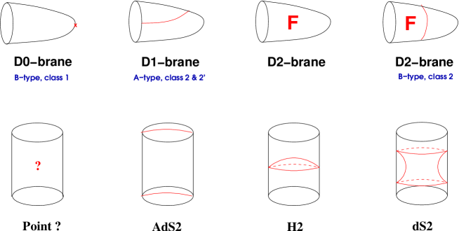
Figure 1: D-branes on the cigar and corresponding $AdS_{3}$ branes

We see that the cigar D1-branes, which descend from $AdS_{2}$ branes in $AdS_{3}$, have two continuous classical moduli, $\theta_{0}$ and $\rho_{min}$. The DBI analysis for the D2-branes that cover the whole cigar implies that they carry a D0-brane charge, which leads to the quantization of the modulus $C$. Since they have trivial topology, they do not admit a non-trivial Wilson line. Finally, for the D2-branes that descend from $dS_{2}$ branes we expect a continuous modulus and the possibility to have a Wilson line due to the nontrivial topology. Notice that in this semiclassical analysis we have not been able to identify the $SL(2,\mathbb{R})$ brane that yields the D0-branes on the cigar. On the other hand, the analysis of [41] has a natural, although geometrically obscure, candidate: the spherical branes of [17] with imaginary radius. These branes preserve the rotational symmetry of the cigar.

The boundary state analysis of the previous sections yields a similar set of branes. The class 1 branes have an open string spectrum that includes only the identity module and they have Dirichlet boundary conditions along $\rho$. The class 2 branes have Neumann boundary conditions in the radial direction. Now, we proceed to analyze in detail each of these boundary states.

5.3 A-type, class 2 and class 2’

These boundary states describe D1-branes extending along the radial direction of the cigar. They have Dirichlet boundary conditions in the $\theta$ coordinate and the simple pole of their wavefunctions at $s^{\prime}=0$ suggests Neumann boundary conditions on $\rho$. This is in line with the interpretation of the ${\cal N}=2$ A-type, class 2 boundary states of [37] as analogues of the FZZT Liouville branes that extend along the Liouville direction [9, 10].

As expected semiclassically, the type-A, class 2 and class 2’ branes possess two branches. In our exact conformal field theory analysis, this is manifest from the computation of the open string spectrum (4.1), (4.1) with $s_{1}=s_{2}$ and $m_{1}=m_{2}$, i.e. for a single D1-brane. This spectrum includes open string states with either integer or half-integer winding $w$. Indeed, these are precisely the spectra encoded in the extended continuous characters $\Lambda^{c}_{\frac{1}{2}+is,0}$ and $\Lambda^{c}_{\frac{1}{2}+is,\frac{k}{2}}$ in the annulus amplitudes (4.1), (4.1).

The class 2’ boundary states are by construction the ones appearing in [41]. The class 2 are closely related. In order to make the comparison with the result of [41] more transparent, we can rewrite the denominator in our class 2 (2’) boundary states in terms of $\Gamma$ functions. With the use of (4.111) and the following identities

$$\Gamma(1+x+iy)\Gamma(1-x+iy)\Gamma(1+x-iy)\Gamma(1-x-iy)=\frac{2\pi^{2}(x^{2}+y^{2})}{\cosh(2\pi y)-\cos(2\pi x)},$$

$$\sinh(\pi x)=\frac{\pi x}{\Gamma(1+ix)\Gamma(1-ix)},$$

we obtain (up to an unimportant phase factor) the class 2 wavefunctions in the form

$$\Psi_{s,m}(s^{\prime},m^{\prime})=\frac{2}{(k(k-2)^{3})^{1/4}}e^{i\delta(m^{\prime})}e^{-\pi i{mm^{\prime}\over k}}\frac{\Gamma(\frac{2is}{k-2})\Gamma(1+2is)}{\Gamma({1\over 2}+{m\over 2}+is)\Gamma({1\over 2}-{m\over 2}+is)}\cos({4\pi ss^{\prime}\over k-2})~{}.$$ (5.165)

The corresponding wavefunctions of [41], which motivated our class 2’ boundary states, read

$$(\Psi^{j}_{n})_{(r,\theta_{0})}=\frac{e^{in\theta_{0}}}{(k(k-2)^{3})^{1/4}}\bigg{(}{\Gamma(1-b^{2})\over\Gamma(1+b^{2})}\bigg{)}^{is}{\Gamma(1+2is)\Gamma(\frac{2is}{k-2})\over\Gamma({1\over 2}+is+{n\over 2})\Gamma({1\over 2}+is-{n\over 2})}\frac{e^{-2irs}+(-1)^{n}e^{+2irs}}{2}~{},$$ (5.166)

where $b^{2}=\frac{1}{k-2}$ and $j=-\frac{1}{2}+is$. Using the identifications

$$\theta_{0} = -\pi\frac{m}{k},$$ (5.167)

$$r = 2\pi\frac{s}{k-2},$$ (5.168)

and setting $n=m^{\prime}+2kl,\;l\in\mathbb{Z},\ m^{\prime}\in\mathbb{Z}_{2k}$, we obtain full agreement between our class 2’ boundary states and (5.166) and partial agreement between the class 2 expression (5.165) and (5.166). Incidentally, notice that the cylinder amplitude (4.17) in [41] can be recast in terms of the extended characters for integer levels $k$, therefore pointing towards the extended Ishibashi states we have been using throughout this paper.

The basic differences between our class 2 D1-branes and those of [41] are the following. First, recall that the latter branes reach the asymptotic circle of the cigar at $\rho\rightarrow\infty$ on two opposite points $\theta_{0}$ and $\theta_{0}+\pi$ and the minimum distance from the tip is parametrized by $r=\rho_{min}\geq 0$. In [41] both of these parameters are continuous. Matching them to the parameters of our boundary state (see eq. (5.167)) shows that our angle $\theta_{0}$ is discrete, because $m\in\mathbb{Z}_{2k}$. Hence, our D1-branes can reach the circle at infinity only at $2k$ special points. This is a simple manifestation of the fact that our branes preserve a larger chiral symmetry than the Virasoro, and it is precisely what one expects from a construction based on extended characters.

The most important difference, however, concerns the coupling of each brane to the closed string modes. The wavefunctions agree for even momentum $n$, but they disagree for odd momentum $n$. This difference affects crucially the semiclassical properties of the class 2 states. In order to make this point clear, we can compare the spectral densities appearing on each class.

First of all, the densities obtained in Section 4 for the class 2’ - class 2’ overlaps should be in perfect agreement with those appearing in [41], if we choose the same regularization scheme. This should be true by construction. Indeed, considering for simplicity the self-overlaps $s_{1}=s_{2}$ and $m_{1}=m_{2}$ and subtracting the spectral densities of a reference brane with $s=0,m=0$, yields the relative spectral densities:

$$\rho_{5}(s^{\prime};s_{1}|s_{1})-\rho_{5}(s^{\prime};0|0)=\frac{1}{2}\Big{(}\rho_{2}(s^{\prime};2s_{1}|0)-\rho_{2}(s^{\prime};0|0)\Big{)}$$ (5.169)

for states with integer winding, and

$$\rho_{6}(s^{\prime};s_{1}|s_{1})-\rho_{6}(s^{\prime};0|0)=\frac{1}{2}\Big{(}\rho_{1}(s^{\prime};2s_{1}|0)-\rho_{1}(s^{\prime};0|0)\Big{)}$$ (5.170)

for states with half-integer winding. It is now a simple exercise to check that under the identification (5.168) and the explicit expressions (4.1) and (4.1) the densities above match (up to a factor of 4 expected from the different normalization of the wavefunctions) with the corresponding relative spectral densities of [41] (relations (4.8), (4.9), (4.10), and (4.11) in that reference). Of course, one needs to perform a summation over $l$ in the result of [41] in order to rewrite it in terms of extended characters.

As has been discussed in [41], the above densities possess the expected semiclassical behavior, i.e. $\rho_{5}(s^{\prime};s_{1}|s_{1})-\rho_{5}(s^{\prime};0|0)$ is finite in the limit $k\rightarrow\infty$, whereas $\rho_{6}(s^{\prime};s_{1}|s_{1})-\rho_{6}(s^{\prime};0|0)$ is not well-defined, because it receives contributions from purely stringy states that decouple in the semiclassical limit. The situation is reversed, however, when we consider the class 2 boundary states. In particular, the regularized density for zero winding (field theory) modes $\rho_{1}(s^{\prime};s_{1}|s_{1})-\rho_{1}(s^{\prime};0|0)$ is ill-defined in the large $k$ limit, implying that the semiclassical interpretation of these boundary states is problematic. This pathology could be an indication that the class 2 branes are unphysical.

In order to elucidate further the physical properties of the class 2 branes, we can compute the semiclassical limit of the one-point functions in the coordinate system introduced in [17] for $H_{3}^{+}$. First, we write the metric of $H_{3}^{+}$ as

$$ds^{2} = d\psi^{2}+\cosh^{2}\psi\;(e^{2\chi}d\nu^{2}+d\chi^{2})$$ (5.171)

$$= d\phi^{2}+e^{2\phi}d\gamma d\bar{\gamma},$$ (5.172)

with $\psi$ an angular coordinate and $\chi,\phi\in[0,\infty)$ radial coordinates. In this coordinate system the $AdS_{2}$ branes are given by surfaces of constant $\psi=r$. They descend, as argued in [17, 41], to D1-branes on the cigar. The one-point function of the resulting branes, ignoring factors unimportant to the present calculation, is conveniently written from (5.166) as

$$(\Psi^{j}_{n})_{(r,\theta_{0})}\sim\Gamma(1+b^{2}(2j+1))\;d^{j}_{n}\;\Big{(}\pi_{n}^{0}\cosh r(2j+1)-\pi^{1}_{n}\sinh r(2j+1)\Big{)},$$ (5.173)

with the definitions:

$$d^{j}_{n} = {\Gamma(2j+1)\over\Gamma(1+j+{n\over 2})\Gamma(1+j-{n\over 2})},$$

$$\pi_{n}^{\epsilon} = \left\{\begin{array}[]{lll}1-\epsilon,&n&:{\rm even},\\ \epsilon,&n&:{\rm odd}.\end{array}\right.$$ (5.176)

Now we can Fourier transform between the $j,n,w$ and the $j,u,\bar{u}$ coordinates using the following formulae [17]:

$$F^{j}_{n,w} = \int_{\mathbb{C}}d^{2}u\;e^{-i\;n\;{\rm arg}(u)}|u|^{2j+kw}f(u),$$ (5.177)

$$f(u) = ik(2\pi)^{-2}\sum_{n\in\mathbb{Z}}\int_{\mathbb{R}}dw\;e^{i\;n\;{\rm arg}(u)}|u|^{-2j-2-kw}F^{j}_{n,w}~{}.$$ (5.178)

One can also show the identity

$$d^{j}_{n}\;\pi^{\epsilon}_{n}\;\delta(w)=(2\pi)^{-2}\int_{\mathbb{C}}d^{2}u\;e^{i\ n\;{\rm arg}(u)}|u|^{-2j-2-kw}|u+\bar{u}|^{2j}{\rm sign}^{\epsilon}(u+\bar{u})~{},$$ (5.179)

which will be used in a moment.

The integral of the Laplace operator eigenfunctions $\Phi^{j}(u|\psi,\chi,\nu)$ [17] over the semiclassical one-point functions gives the geometrical shape of the corresponding D-brane. For the $AdS_{2}$ branes and by using (5.179), this computation yields

$$\int dj\int d^{2}u\;\Big{(}\Phi^{j}(u|\psi,\chi,\nu)\Big{)}^{*}|u+\bar{u}|^{2j}\Big{(}\cosh r(2j+1)-{\rm sign}(u+\bar{u})\sinh r(2j+1)\Big{)}\sim\delta(\psi-r),$$ (5.180)

therefore describing a D1-brane as in Table 1.

One can determine the shape of the class 2 boundary states in the semiclassical limit in a similar way. First we need to write down the corresponding wavefunctions in a form similar to (5.173):

$$(\Psi^{j}_{n})^{\prime}_{(r,\theta_{0})}\sim\Gamma(1+b^{2}(2j+1))\;d^{j}_{n}\;\Big{(}\pi_{n}^{0}\cosh r(2j+1)-i\pi^{1}_{n}\cosh r(2j+1)\Big{)}.$$ (5.181)

Integrating them as above with the use of the eqs. (5.177) and (5.179) gives

$$\int dj \int d^{2}u\;\Big{(}\Phi^{j}(u|\psi,\chi,\nu)\Big{)}^{*}|u+\bar{u}|^{2j}\Big{(}\cosh r(2j+1)-i\;{\rm sign}(u+\bar{u})\cosh r(2j+1)\Big{)}\sim$$

$$\int_{0}^{\infty} dP \Big{(}\sin 2P(\psi+r)+\sin 2P(\psi-r)\Big{)}+\delta(\psi-r)+\delta(\psi+r).$$ (5.182)

The integral in the second line comes from the term involving ${\rm sign}(u+\bar{u})$ and it can be traced back to the contribution of odd momenta to $\pi_{n}^{1}$. This integral is not well defined and does not lead to a sensible geometrical interpretation of the class 2 D1-branes.

A possible way out is to consider a linear combination of the A-type class 2 wavefunction (3.87) with its complex conjugate, in particular $(\Psi^{j}_{n})^{even}_{(r,\theta_{0})}=(\Psi^{j}_{n})_{(r,\theta_{0})}+(\Psi^{j}_{n})_{(r,\theta_{0})}^{*}$. In this case, the only non-zero couplings to closed strings are the ones with even momentum $n$. As a consequence, we only get the $\delta$ function terms in (5.3). This boundary state describes two D1-branes with parameters $(r,\theta_{0})$ and $(-r,\theta_{0})$. This, however, is exactly the same boundary state that one would obtain from a linear superposition of two D1-branes of [41]. Therefore, it seems that employing the Cardy ansatz does not lead to D1-branes with nice semiclassical features and we are probably left only with the class 2’ branes of [41].

Finally, we can check if the class 2 states satisfy the $H_{3}$ factorization constraints derived in [17]. It was shown there that the allowed one-point functions for the $AdS_{2}$ branes (and correspondingly for their descendants on the cigar), have the following form

$$(\Psi^{j}(u|{i\over 2}))_{r}=|u+\bar{u}|^{2j}\nu_{b}^{j+{1\over 2}}\Gamma(1+b^{2}(2j+1))E_{\sigma}(j|r)$$ (5.183)

with $\nu_{b}$ a normalization constant and $\sigma={\rm sign}(u+\bar{u})$. The function $E_{\sigma}(j|r)$ is restricted by factorization constrains to have the form

$$E_{\sigma}(j|r)=(e^{0}(j|r)+e^{1}(j|r)\sigma)e^{-r(2j+1)\sigma},$$ (5.184)

with $e^{\epsilon}(-1-j|r)=(-1)^{\epsilon}e^{\epsilon}(j|r)$. The general A-type, class 2 boundary state with Fourier transformed wavefunction (5.181) is not of the above form and hence does not solve the $H_{3}$ factorization constrains. It would be an important but challenging task to determine the consistency of these boundary states by analyzing the factorization constraints directly in the cigar conformal field theory.

5.4 B-type, class 1

We find a single B-type, class 1 brane. This boundary state has Neumann boundary conditions on the angular direction of the cigar (it is B-type) and is localized in the radial direction (it is class 1). A circular D1-brane wrapped around the cigar will slip towards the tip to lower its energy. Therefore, our B-type, class 1 brane will eventually be localized at the tip of the cigar, where it should rather be interpreted as a D0-brane. Perhaps it is useful to think of this brane as the analog of the $SU(2)/U(1)$ B-type brane with $j=0$ that sits at the center of the $SU(2)/U(1)$ disk [5]. However, unlike those branes, which are unstable and can move away from the center of the disk, the D0-brane of the cigar is stable and cannot move from the tip. Analogous branes were formulated for the cigar CFT in [41]. These branes were parametrized by a single discrete parameter $m=1,2,...$, but as explained in that paper, only the $m=1$ brane appeared to be physical. A comparison of the properties of our B-type, class 1 brane with those of the $m=1$ brane of [41] below indicates that these are the same branes. Notice that we have restricted our analysis only to unitary representations. As a result, our approach does not yield the $m>1$ boundary states of [41], which carry non-unitary open string spectra.

The B-type, class 1 boundary state couples to both continuous and discrete closed string modes. The appropriate wavefunctions are listed in eqs. (5.151)-(5.154) and they are in agreement with the expressions appearing in [41]. For the continuous part the wavefunctions read:

$$\Psi(j,w)_{m=1}^{D0}=(-)^{w}(k(k-2))^{1/4}\Big{(}{\Gamma(1-b^{2})\over\Gamma(1+b^{2})}\Big{)}^{j+\frac{1}{2}}\frac{\Gamma(-j+\frac{kw}{2})\Gamma(-j-\frac{kw}{2})}{\Gamma(-b^{2}(2j+1))\Gamma(-2j)}~{}.$$ (5.185)

where $b^{2}={1\over k-2}$ and $j=-{1\over 2}+is$ in the notation of [41]. Indeed, up to a phase factor that does not affect the analysis of the cylinder amplitudes, we find that these wavefunctions depend on $w$ only through its parity (i.e. on whether $w$ is even or odd). With a few straightforward algebraic manipulations one can show that they can be brought into the form

$$\Phi(s,a)=(k(k-2))^{1/4}\Big{(}{\Gamma(1-b^{2})\over\Gamma(1+b^{2})}\Big{)}^{is}\frac{\Gamma({1\over 2}+\frac{ak}{2}-is)\Gamma({1\over 2}-\frac{ak}{2}-is)}{\Gamma(-b^{2}2is)\Gamma(1-2is)}~{},$$ (5.186)

with $a=0,~{}1$. Similarly, for the discrete representations one obtains the wavefunctions

$$D(j,{ak\over 2}-j)=\sqrt{2}\bigg{(}\frac{k}{k-2}\bigg{)}^{1/4}\sqrt{\sin(-b^{2}\pi(2j+1))}~{}.$$ (5.187)

The above wavefunctions yield a cylinder amplitude $\langle B|e^{-\pi TH^{c}}|B\rangle$, which agrees with the result following from eqs. (5.151)-(5.154). There is a small difference in the contribution of the discrete representations, which we now flesh out.

The discrete part of the above cylinder amplitude involves a summation over the quantum numbers $j$ and $w$. In [41] (see eq. (3.18)) this summation runs over the restricted set ${\cal J}^{d}_{0,w}:=\big{[}\frac{1}{2},\frac{k-1}{2}\big{]}\cap\big{(}\frac{1}{2}|kw|-\mathbb{N}\big{)}$. Our result involves a similar summation over $j$ and $w$, but ${\cal J}^{d}_{0,w}$ should be replaced by the unrestricted interval $\big{(}\frac{1}{2},\frac{k-1}{2}\big{)}$. Notice, however, that this difference affects only the $w=0$ contribution. Indeed, we are dealing with even levels $k$, so can set $k=2\nu$, where $\nu$ is some positive integer. Then, the condition that $j$ belongs in ${\cal J}^{d}_{0,w}$ requires the existence of a positive integer $n$, such that $j=-n+1/2|kw|=-n+\nu|w|$ and such that it satisfies the inequality $1/2+\nu(|w|-1)\leq n\leq\nu|w|-1/2$. $n$ will be necessarily positive for any $k>2$. It should be clear that for each $w\in\mathbb{Z}^{*}$ we can always find an appropriate integer $n$ in the range defined above and for such $n$’s we get the same values of $j$ for every possible non-vanishing value of $w$. The value $w=0$ is the only exception. It is therefore excluded in the computation of [41], but it is included in our computation. Unfortunately, we cannot offer an explanation for this discrepancy.

Despite this minor difference, the cylinder amplitudes agree perfectly in the open string channel. The result appearing in (4.127) can be recast in terms of the standard $\lambda^{d}_{j,r}$ discrete characters, using the identity (C.259). One finds:

$$\sum_{r\in\mathbb{Z}_{k}}\Lambda^{I}_{r}(\tau)=\sum_{l\in\mathbb{Z}}(\lambda^{d}_{0,l}(\tau)-\lambda^{d}_{1,l-1}(\tau))=q^{-\frac{c_{cs}}{24}}\Big{(}1+2q^{1+{1\over k}}+q^{2}+O(q^{2+{1\over k}})\Big{)}~{}.$$ (5.188)

In this expression $\lambda^{d}_{0,n}$ denotes the extrapolation of the discrete character (2.5) to $j=0$ and not the character (2.4) of the identity representation. This is precisely the result found in eq. (3.6) of [41].

As we see, the open string spectrum of the B-type, class 1 brane is discrete and there is no open string winding. This is a simple manifestation of the fact that the B-type, class 1 brane is rotationally invariant. For finite level $k$ the one-loop result in (5.188) suggests that the open string spectrum does not contain any marginal modes. This is consistent with the semiclassical analysis, which fixes the position of the D0-brane at the tip of the cigar. In the flat space limit, however, two states with scaling dimension $h=1$ appear signaling the free motion of a D0-brane in a flat 2-dimensional space.

5.5 B-type, class 2

These branes are new and have not been considered before in the boundary conformal field theory context. They are labeled by a continuous parameter $s\in[0,\infty)$ and they have Neumann boundary conditions both in the angular and radial directions. Hence, their shape is that of 2-dimensional D-branes. Since they do not couple to any discrete modes, which are localized near the tip of the cigar, it is natural to expect that in general these branes do not reach the tip and hence they are candidates for the D2-branes descending from $dS_{2}$ branes of $AdS_{3}$ in Table 1. Such branes develop a circular opening at a distance $\rho_{min}$ away from the tip and terminate there. The parameter $\rho_{min}$ is directly related to the continuous parameter $s$. For example, we can easily verify that both parameters scale to infinity when we send $k\rightarrow\infty$. For finite $k$ notice that when we send $s\rightarrow 0$, the circular opening of the D2-brane shrinks to zero radius and the brane covers the whole cigar.

According to the semiclassical analysis of subsection 5.2 these D2-branes can have a non-vanishing $\mathbb{Z}_{2}$ Wilson line because of the non-trivial cycle on their worldvolume. The anticipation of a $\mathbb{Z}_{2}$-valued, instead of $\mathbb{R}$-valued, Wilson line will be better clarified in a moment with the use of a T-duality argument. The possibility of the Wilson line is realized explicitly by our B-type, class 2 branes. The one-point functions in (3.97) depend on the extra $\mathbb{Z}_{2}$-valued parameter $\alpha=0,~{}\frac{1}{2}$. The Cardy computation in (4.130) shows clearly that the overlap of two branes with the same values $\alpha_{1}=\alpha_{2}$ results in open string states with even index $m$. On the other hand, the same computation for branes with different values of $\alpha_{1}$ and $\alpha_{2}$ involves open string states with odd $m$. The explicit form of the extended character $\Lambda^{c}_{{1\over 2}+is,\ {m\over 2}}$ in (C.253) reveals that even $m$ indices correspond to integer momentum modes in the angular direction, whereas odd $m$ indices correspond to half-integer momentum modes. Therefore, this open string spectrum suggests that $\alpha$ parameterizes a $\mathbb{Z}_{2}$ Wilson line. It is known (see e.g. [67]) that if we have a circular D1 string, the presence of a $\mathbb{Z}_{2}$ Wilson line results, under a $2\pi$ translation around the $S^{1}$, into a minus sign in the wavefunction of an open string ending on the D1-string. In our case, that would imply half-integer angular momenta for open strings stretching between an $\alpha=0$ and an $\alpha=\frac{1}{2}$ brane. As a consequence, in the field theory limit one would expect, for example, a tachyon field of the form [67]:

$$T(\theta,\rho)=\sum_{n\in\mathbb{Z}}T_{n}(\rho)e^{i(n+{1\over 2})\theta}~{}.$$ (5.189)

Indeed, this is what we observe in the open string spectra of our branes. Eq. (C.253) with $s=0$ and $m=2n+1$ ($n\in\mathbb{Z}$) shows that the open string spectrum includes $l=0$ modes with scaling dimensions $h={(n+{1\over 2})^{2}\over k}$. In the semiclassical limit of large $k$ these are precisely the scaling dimensions of tachyon modes with half-integer angular momentum on a circle of radius $\sqrt{k}$.

The $\mathbb{Z}_{2}$ Wilson line can also be derived by the following T-duality argument. As we briefly mentioned in Section 2, the trumpet geometry can be obtained from the cigar by T-duality. This T-dual background can also be viewed as a $\mathbb{Z}_{k}$ orbifold of the cigar. This is most apparent in the asymptotic cylinder region, where the $Z_{k}$ orbifold reduces the asymptotic radius $R_{cig}$ to $R_{cig}/k$. To avoid the subtleties due to the singularity in the trumpet geometry we can restrict our discussion only on the asymptotic cylinder region. On the trumpet we can formulate D1-branes, which are the analogs of the A-type, class 2 (2’) branes on the cigar (see [40]). Again, these branes will be parameterized by a continuous parameter $s$ and geometrically will correspond to D1-branes starting from the asymptotic infinity and returning back to it. They will be perturbative and stay far from the trumpet singularity for large parameters $s$. The boundary states of these D1-branes can be deduced easily from the analysis of the A-type, class 2 (2’) branes on the cigar. They are simply $\mathbb{Z}_{k}$ orbifold projections of those branes. In other words, they can be obtained by summing over $k$ images of the A-type, class 2 (2’) boundary states. To be definite, let us consider only the A-type, class 2’ cigar branes, which have better semiclassical behavior. There are two possible sums over $k$ images that we can write and one can easily show that:

$$|A;s,1\rangle_{trumpet}\equiv\frac{1}{\sqrt{k}}\sum_{l\in\mathbb{Z}_{k}}|A;s,l\rangle=\frac{1}{2}|B;s,\alpha=0\rangle~{},$$ (5.190)

$$|A;s,2\rangle_{trumpet}\equiv\frac{1}{\sqrt{k}}\sum_{l\in\mathbb{Z}_{k}}|A;s,l+\frac{1}{2}\rangle=\frac{1}{2}|B;s,\alpha=\frac{1}{2}\rangle~{}.$$ (5.191)

This result is precisely what we expect from T-duality. The A-type trumpet D1-branes were expected to yield B-type D2-branes on the cigar and this is exactly what we find. The Wilson line is naturally $\mathbb{Z}_{2}$-valued, because there are only $2k$ D1-branes on the cigar and the $\mathbb{Z}_{k}$ orbifold leaves behind a remaining $\mathbb{Z}_{2}$ degree of freedom. Hence, the fact that we do not have an $\mathbb{R}$-valued Wilson line, as would be expected on geometric grounds, can be traced back to the use of extended Ishibashi states that preserve more symmetry than just the Virasoro.

As a final comment on the B-type class 2 branes notice that the self overlaps in (4.130) yield an open string spectrum that has a marginal deformation for $s=\sqrt{k-2}$ and $m=0$. This indicates that our D2-branes are marginally stable to a change of the $s$ modulus. Such a marginal mode is also expected from the semiclassical analysis. The DBI action has a flat direction of solutions parameterized by $\rho_{min}$. Moreover, one can compute the radial stress energy tensor component $T_{\rho\rho}$:

$$T_{\rho\rho}={\partial{\cal L}\over\partial F_{\rho\theta}}F_{\rho\theta}-{\cal L}=T_{D2}\Bigg{(}{\cosh\rho(F_{\rho\theta})^{2}\over\sqrt{\tanh^{2}\rho+(F_{\rho\theta})^{2}}}-\cosh\rho\sqrt{\tanh^{2}\rho+(F_{\rho\theta})^{2}}\Bigg{)}$$ (5.192)

and show, using the equations of motion from Table 1, that it is zero (and therefore continuous) at the minimum distance from the tip $\rho_{min}$. This provides further confirmation for the existence of the above marginal deformation.

5.6 B-type, class 3

The analysis of Section 4 revealed that the class 3 (and most of the class 3’) boundary states have negative open string multiplicities and hence do not satisfy the Cardy consistency conditions. Nevertheless, there are some striking similarities between the class 3’ boundary states of this paper and the cigar covering D2-branes of [41] and it is instructive to compare the two results. For those branes we use the form of the closed string couplings that appear in [43]

$$\langle\Phi^{j}_{w}({i\over 2},-{i\over 2})\rangle = {b^{2}\over 4}(\nu_{b})^{j+{1\over 2}}{\Gamma(j+{kw\over 2})\Gamma(j-{kw\over 2})\over\Gamma(2j-1)\Gamma(1-(2j-1)b^{2})}$$

$${e^{i\sigma(2j-1)}\sin\pi(j+{kw\over 2})+e^{-i\sigma(2j-1)}\sin\pi(j-{kw\over 2})\over\sin\pi(2j-1)\sin\pi b^{2}(2j-1)}=$$

$$= 2(-1)^{{kw\over 2}}{b^{2}\over 4}(\nu_{b})^{j+{1\over 2}}{\Gamma(j+{kw\over 2})\Gamma(j-{kw\over 2})\sin\pi j\cos\sigma(2j-1)\over\Gamma(2j-1)\Gamma(1-(2j-1)b^{2})\sin\pi(2j-1)\sin\pi b^{2}(2j-1)}~{}.$$

For $2j_{1}=(k-2){\sigma\over\pi}+{k\over 2}$, and $2j_{2}=-(k-2){\sigma\over\pi}+{k\over 2}$, the class 3’ boundary state wavefunctions (3.101)-(3.104) become:

$$\Phi_{j_{1},j_{2}}(s,0) = 2\bigg{(}{k\over k-2}\bigg{)}^{{1\over 4}}{\cosh 2\sigma s\over\sqrt{\sinh 2\pi sb^{2}\sinh 2\pi s}}~{},$$ (5.194)

$$\Phi_{j_{1},j_{2}}(s,k) = 2\bigg{(}{k\over k-2}\bigg{)}^{{1\over 4}}e^{i\pi{k\over 2}}{\cosh 2\sigma s\over\sqrt{\sinh 2\pi sb^{2}\sinh 2\pi s}}~{},$$ (5.195)

$$D_{j_{1},j_{2}}(j,-j) = 2{i\over\sqrt{2}}\bigg{(}{k\over k-2}\bigg{)}^{{1\over 4}}{1\over\sqrt{\sin\pi b^{2}(2j-1)}}e^{{i\pi\over 2}(2j-1)}\cos\sigma(2j-1)~{},$$ (5.196)

$$D_{j_{1},j_{2}}(j,{k\over 2}-j) = 2{i\over\sqrt{2}}\bigg{(}{k\over k-2}\bigg{)}^{{1\over 4}}{1\over\sqrt{\sin\pi b^{2}(2j-1)}}e^{{i\pi\over 2}(2j-1)}e^{i\pi{k\over 2}}\cos\sigma(2j-1)~{}.$$ (5.197)

Notice that since $1\leq 2j_{i}\leq k-1$ we can easily obtain the quantization condition $\sigma=\pi{m\over k-2}$ with the bound $\sigma\in[0,{\pi\over 2})$.

It is not difficult to compare the above couplings with those of (5.6). One finds that the continuous couplings are the same except for several phase factors that do not affect the cylinder amplitudes. The discrete couplings, on the other hand, appear to be different. This should be expected. From a similar comparison involving the B-type class 1 branes [41], we know that for discrete representations properly normalized one-point functions should be considered. More precisely, in computing the cylinder amplitudes using (5.6) one has to consider discrete contributions of the form:

$$\sum_{w,j}{\rm Res}\bigg{(}{\Psi_{\sigma}(j,w)\Psi_{\sigma}(j,w)^{*}\over\langle\Phi^{j}_{0,w}\Phi^{j}_{0,w}\rangle}\bigg{)}\lambda^{d}_{j,\frac{kw}{2}}(iT)~{},$$ (5.198)

where one uses the bulk two-point function of the operator $\Phi^{j}_{0,w}$ to normalize the cylinder contributions for each closed string mode. It should be obvious from the last equation in (5.6) that the dependence on $\sigma$ is the same as that in (5.194). Moreover, the $\Gamma$ functions in the numerator of (5.6) exhibit discrete poles for $j\pm{kw\over 2}=-n,\ n\in\mathbb{N}$. For even levels $k$ this yields contributions from all the $integer$ values of $j\in\big{[}\frac{1}{2},\frac{k-1}{2}\big{]}$, precisely as expected from the cylinder amplitude computation of section 4.

Despite the apparent similarity of the above one-point functions, the expression (4.140) for the self-overlap differs from the annulus amplitude computed in [41, 43]. In particular, these papers find that the contribution of discrete open string states vanishes in the case of self-overlaps. This result is in contrast to (4.140) except for $\sigma=\pm\frac{\pi}{2}$, in which case our class 3 B-type boundary states reduce to class 2 boundary states. This vanishing, combined with the negative open string multiplicities of the remaining cross-overlaps, led the authors of [43] to conclude that only a single D2-brane should be allowed.

We should point out, however, that the analysis of [41, 43] is, strictly speaking, valid only for non-rational levels $k$. For rational levels there are additional subleties involving contributions due to extra poles, which were not taken into account in the discussion of [41, 43]. Hence, it is plausible that the results of those papers might not apply directly to the case of integer levels $k$ that we study in this work. If this is the case, then it would be interesting to see if the extra pole contributions can explain the discrepancy between our results and those appearing in [41, 43].

6 Summary and conclusions

In this paper we formulated D-branes on the $SL(2,\mathbb{R})_{k}/U(1)$ coset conformal field theory at integer level $k$. The basic building blocks of our analysis were the extended coset characters of [39]. With the use of the corresponding extended Ishibashi states we proposed Cardy-like boundary states and verified the Cardy consistency conditions. Although the discussion we presented here applies directly only to integer levels $k$, the extension to rational levels should be straightforward.

Our analysis yielded the following results. We found two basic types of boundary states: A- and B-type. We presented two A-type boundary states, which we called class 2 and class 2’. Both of them are based on the continuous representations and geometrically correspond to D1-branes starting and terminating at the asymptotic infinity. The class 2 boundary states resulted from a direct application of the Cardy ansatz and exhibit some puzzling semiclassical features. It is not completely clear whether these branes are fully consistent. The class 2’ boundary states are a slight variant of the Cardy ansatz and they have appeared previously in [41], where they were derived from $AdS_{2}$ boundary states in the Euclidean $AdS_{3}$. These branes have the expected semiclassical behavior.

We also presented two classes of B-type boundary states. These were called class 1 and class 2. We found a single B-type class 1 boundary state, which is based on the identity representation and corresponds to a rotationally invariant D1-brane that wraps the circular direction of the cigar and slips toward the tip in order to minimize its energy. In this way it becomes effectively a pointlike object, i.e. a D0-brane. The class 2 branes are based only on continuous representations and they are D2-branes (with a $\mathbb{Z}_{2}$-valued Wilson line) covering part of the cigar (see Fig. 1). An interesting question concerns the formulation of D2-branes covering the whole cigar. These are expected to be based on the discrete representations. We formulated such branes in Section 3 as class 3 boundary states, but they were found in Section 4 to violate the Cardy consistency conditions and they had to be excluded. Nevertheless, it would still be interesting to see if one can postulate Cardy consistent class 3 boundary states as appropriate linear combinations of the class 3 boundary states of Section 3, or with wavefunctions that do not follow from the application of the Cardy ansatz. The simple linear superposition that yielded the class 3’ boundary states produced a set of D2-branes that share many similarities with the cigar covering D2-branes of refs. [41, 43]. Only one of them was found, however, to be Cardy consistent. A similar observation was made in [43].

In conclusion we would like to mention a few open problems. The analysis we presented was based exclusively on the study of the Cardy consistency conditions. Hence, it should be supplemented by a detailed study of the disk 1-point function factorization constraints. This would provide additional evidence for the results presented in this paper and would clarify important aspects of the open string theory on the D-branes we considered. The analysis of the 4-point function conformal blocks is expected to be the difficult part of this task. Another related task would be the study of the boundary two- and three-point functions of the open string theories presented here.

Moreover, it would be intriguing to study the implications of our results for two-dimensional holography and the connection with the matrix model of [36] in the spirit of [32, 33, 34]. On a related context, one could also explore the possibility of deriving the connection to the matrix model through an auxiliary Riemann surface similar to the analysis that has been performed for the minimal (super)string theory in [68].

Finally, it would be worthwhile to obtain boundary states for the supersymmetric orbifold

$$\frac{SL(2,\mathbb{R})_{k}/U(1)\times SU(2)_{k}/U(1)}{\mathbb{Z}_{k}}$$ (6.199)

by extending the techniques used here. This background appears in the exact CFT description of NS5-branes (put symmetrically on a topologically trivial circle) and provides a holographic dual of Little String Theory in the double scaling limit [30]. It is therefore of obvious importance to understand the corresponding D-branes. Furthermore, analyzing the dynamics of these branes along the lines of [69] and in connection with Hanany-Witten type configurations [70, 71] is another interesting open problem.

Appendix A The coset partition sum in terms of standard and extended characters

The spectrum of string theory on the axially-gauged (cigar) coset involves only the continuous and discrete representations. For a semiclassical discussion of this spectrum we refer the reader to [25]. A more recent discussion, from the point of view of the torus partition sum, can be found in [52]. In this Appendix we review the basic features of that computation and show explicitly how the torus partition sum can be recast in terms of the standard and extended characters. The standard character form did not appear explicitly in [52], but it was already implicit in the considerations of that paper. The supersymmetric version of the partition sum expression in terms of extended characters appeared recently in [53, 54].

Our starting point is the torus partition sum (3.9) of [52]:

$${\cal Z}(\tau,\bar{\tau}) = 2(k(k-2))^{1/2}\int_{0}^{1}ds_{1}ds_{2}$$

$$\sum_{m,w\in\mathbb{Z}}\frac{(q\bar{q})^{-2/24}}{|\sin(\pi(s_{1}\tau-s_{2}))|^{2}}\frac{e^{-\frac{k\pi}{\tau_{2}}|(s_{1}+w)\tau-(s_{2}+m)|^{2}+\frac{2\pi}{\tau_{2}}(\Im(s_{1}\tau-s_{2}))^{2}}}{\displaystyle|\prod_{r=1}^{\infty}(1-e^{2\pi ir\tau-2\pi i(s_{1}\tau-s_{2})})(1-e^{2\pi ir\tau+2\pi i(s_{1}\tau-s_{2})})|^{2}}~{}.$$

This result can be derived from a direct path integral computation in the corresponding gauged WZW theory.

With the use of the Poisson resummation formula in $m$ it is possible to recast (A) into the form

$${\cal Z}(\tau,\bar{\tau}) = 8\sqrt{(k-2)\tau_{2}}|\eta(\tau)|^{2}\int_{0}^{1}ds_{1}ds_{2}\frac{e^{2\pi\tau_{2}s_{1}^{2}}}{|\theta_{1}(s_{1}\tau-s_{2}|\tau)|^{2}}$$ (A.201)

$$\sum_{n,w\in\mathbb{Z}}e^{2\pi ins_{2}}q^{\frac{1}{4k}(n-k(w+s_{1}))}\bar{q}^{\frac{1}{4k}(n+k(w+s_{1}))^{2}}~{},$$

where

$$\theta_{1}(z|\tau)=-2e^{\pi i\tau/4}\sin\pi z\prod_{m=1}^{\infty}(1-q^{m})(1-e^{2\pi iz}q^{m})(1-e^{-2\pi iz}q^{m})~{}.$$ (A.202)

We can expand this function in the denominator of the partition sum, with the help of the formula ($y=e^{2\pi i(s_{1}\tau-s_{2})}$)

$$\frac{1}{\theta_{1}(s_{1}\tau-s_{2}|\tau)}=\frac{iy^{1/2}}{\eta^{3}(\tau)}\sum_{r\in\mathbb{Z}}y^{r}S_{r}(\tau)~{},$$ (A.203)

where

$$S_{r}(\tau)=\sum_{s=0}^{\infty}(-)^{s}q^{\frac{1}{2}s(s+2r+1)}~{}.$$ (A.204)

This expansion is valid only for $|q|<|z|<1$, which is indeed the case for $0<s_{1}<1$.

Plugging the expansion (A.203) into the partition sum (A.201) and integrating out $s_{2}$ yields

$${\cal Z}(\tau,\bar{\tau}) = 8\sqrt{(k-2)\tau_{2}}\frac{1}{|\eta(\tau)|^{4}}\int_{0}^{1}ds_{1}\sum_{r,\bar{r},w\in\mathbb{Z}}e^{2\pi\tau_{2}(\frac{k-2}{2}s_{1}^{2}+s_{1}(1+r+\bar{r}+kw))}$$ (A.205)

$$q^{\frac{1}{4k}(r-\bar{r}-kw)^{2}}\bar{q}^{\frac{1}{4k}(r-\bar{r}+kw)^{2}}S_{r}(\tau)S_{\bar{r}}(\bar{\tau})~{},$$

with the constraint $n=r-\bar{r}$. Following [52] we can introduce an auxiliary variable $s$ to linearize the $s_{1}$ integral. This can be achieved with the use of the identity

$$\sqrt{(k-2)\tau_{2}}e^{-2\pi\tau_{2}(\frac{k-2}{2}s_{1}^{2}+s_{1}(1+r+\bar{r}+kw))}=\int_{-\infty}^{\infty}ds~{}e^{-\frac{\pi s^{2}}{(k-2)\tau_{2}}-2\pi s_{1}(is+\tau_{2}(1+r+\bar{r}+kw))}~{}.$$ (A.206)

Then, we can easily perform the $s_{1}$ integral to obtain the partition sum in the form

$${\cal Z}(\tau,\bar{\tau}) = \frac{8}{|\eta(\tau)|^{4}}\int_{-\infty}^{\infty}ds~{}\sum_{r,\bar{r},w\in\mathbb{Z}}q^{\frac{1}{4k}(r-\bar{r}-kw)^{2}}\bar{q}^{\frac{1}{4k}(r-\bar{r}+kw)^{2}}S_{r}(\tau)S_{\bar{r}}(\bar{\tau})$$ (A.207)

$$\frac{e^{-\frac{\pi}{(k-2)\tau_{2}}s^{2}}}{2\pi(is+\tau_{2}(1+r+\bar{r}+kw))}\bigg{(}1-e^{-2\pi(is+\tau_{2}(1+r+\bar{r}+kw))}\bigg{)}~{}.$$

In the above expression, the contribution of the discrete representations comes from the second term. The exponent of the exponential inside the parenthesis can be completed to a square by shifting $s$ and by defining the new variable $t=s+i(k-2)\tau_{2}$ we can write the second term as

$$- \frac{4}{i\pi|\eta(\tau)|^{4}}\int_{{\cal C}}dt~{}\sum_{r,\bar{r},w\in\mathbb{Z}}q^{\frac{1}{4k}(r-\bar{r}-kw)^{2}}\bar{q}^{\frac{1}{4k}(r-\bar{r}+kw)^{2}}S_{r}(\tau)S_{\bar{r}}(\bar{\tau})$$ (A.208)

$$e^{-\frac{\pi}{(k-2)\tau_{2}}t^{2}}e^{-2\pi\tau_{2}(\frac{k}{2}+r+\bar{r}+kw)}\frac{1}{t-i\tau_{2}(k-1+r+\bar{r}+kw)}~{},$$

where ${\cal C}$ denotes the contour ${\cal C}=\{t|t=s+i\tau_{2}(k-2),s\in\mathbb{R}\}$. We may close the contour at $\pm\infty$ to form an infinite parallelogram between the real line and ${\cal C}$. Then, the integrand has poles at the locations $t=i\tau_{2}(k-1+r+\bar{r}+kw)$ inside the parallelogram, i.e. it has poles for those integers $r$, $\bar{r}$ and $w$ for which $0<k-1+r+\bar{r}+kw<k-2$. The contribution of these poles gives the contribution ${\cal Z}_{d}$ of the discrete representations to the torus partition sum. After setting $2j\equiv-kw-r-\bar{r}$ it is straightforward to show that

$${\cal Z}_{d}(\tau,\bar{\tau})=8\sum_{\frac{1}{2}<j<\frac{k-1}{2}}\sum_{w,r,\bar{r}\in\mathbb{Z}}\delta(2j+r+\bar{r}+kw)\lambda^{d}_{j,r}(\tau)\lambda^{d}_{j,\bar{r}}(\bar{\tau})~{}.$$ (A.209)

Since we assume that $k$ is an (even) integer we see that $2j\in\mathbb{Z}$. Notice that in principle we can replace $\lambda^{d}_{j,r}$ by $\lambda^{d}_{\frac{k}{2}-j,-r}$ since they share the same conformal weights. However, their respective $J_{0}^{3}$ charges are different and choosing the second one would not lead to a sensible interpretation of these charges as left- and right-moving momenta of a free compact boson, which is required by the BRST constraint of the corresponding gauged WZW model. In general one can check that the discrete part cannot be written in terms of characters with $j\neq\bar{j}$. This will be important when we discuss the allowed coset Ishibashi states.

The contribution of the continuous representations can be obtained in a similar way. The integral over the first term in (A.207) plus the integral along the real line that remains from (A.208) give

$${\cal Z}_{c}(\tau,\bar{\tau}) = \frac{16}{|\eta(\tau)|^{4}}\int_{-\infty}^{\infty}\frac{ds}{2\pi}\sum_{r,\bar{r}\in\mathbb{Z}}\sum_{n,w\in\mathbb{Z}}\delta_{r-\bar{r},n}\;q^{\frac{s^{2}}{k-2}+\frac{1}{4k}(n-kw)^{2}}\bar{q}^{\frac{s^{2}}{k-2}+\frac{1}{4k}(n+kw)^{2}}S_{r}(\tau)S_{\bar{r}}(\bar{\tau})$$ (A.210)

$$\Big{(}\frac{1}{2is+r+\bar{r}+kw+1}-\frac{(q{\bar{q}})^{\frac{1}{2}(\frac{k}{2}+r+\bar{r}+kw)}}{2is+r+\bar{r}+k(w+1)-1}\Big{)}.$$

Compared to (A.207) and (A.208) we have rescaled the integration variable as $s\rightarrow 2\tau_{2}s$. This expression can also be written as

$${\cal Z}_{c}(\tau,\bar{\tau})=\frac{16}{|\eta(\tau)|^{4}}\int_{-\infty}^{\infty}\frac{ds}{2\pi}\sum_{r,\bar{r}\in\mathbb{Z}}\sum_{n,w\in\mathbb{Z}}\delta_{r-\bar{r},n}\;S_{r}(\tau)S_{\bar{r}}(\bar{\tau})$$

$$\Bigg{(}\frac{q^{\frac{s^{2}}{k-2}+\frac{1}{4k}(n-kw)^{2}}\bar{q}^{\frac{s^{2}}{k-2}+\frac{1}{4k}(n+kw)^{2}}}{2is+r+\bar{r}+kw+1}-\frac{q^{\frac{s^{2}}{k-2}+\frac{1}{4k}(n-k(w+1))^{2}+r}+\bar{q}^{\frac{s^{2}}{k-2}+\frac{1}{4k}(n+k(w+1))^{2}+\bar{r}}}{2is+r+\bar{r}+k(w+1)-1}\Bigg{)}.$$

Shifting $w\rightarrow w-1$ in the second term and using the relation $q^{r}S_{r}=S_{-r}$ yields

$${\cal Z}_{c}(\tau,\bar{\tau}) = \frac{16}{|\eta(\tau)|^{4}}\int_{-\infty}^{\infty}\frac{ds}{2\pi}\sum_{r,\bar{r}\in\mathbb{Z}}\sum_{n,w\in\mathbb{Z}}\delta_{r-\bar{r},n}\;q^{\frac{s^{2}}{k-2}+\frac{1}{4k}(n-kw)^{2}}\bar{q}^{\frac{s^{2}}{k-2}+\frac{1}{4k}(n+kw)^{2}}$$ (A.212)

$$\Big{(}\frac{S_{r}S_{\bar{r}}}{2is+r+\bar{r}+kw+1}-\frac{S_{-r}S_{-\bar{r}}}{2is+r+\bar{r}+kw-1}\Big{)}.$$

This result can be simplified further with the use of the identity $S_{-r}=1-S_{r-1}$ and by shifting $r\rightarrow r+1,\bar{r}\rightarrow\bar{r}+1$ in the second term. This allows us to bring the above expression into the form

$${\cal Z}_{c}(\tau,\bar{\tau}) = \frac{16}{|\eta(\tau)|^{4}}\int_{-\infty}^{\infty}\frac{ds}{2\pi}\sum_{r,\bar{r}\in\mathbb{Z}}\sum_{n,w\in\mathbb{Z}}\delta_{r-\bar{r},n}$$ (A.213)

$$q^{\frac{s^{2}}{k-2}+\frac{1}{4k}(n-kw)^{2}}\bar{q}^{\frac{s^{2}}{k-2}+\frac{1}{4k}(n+kw)^{2}}\frac{S_{r}+S_{\bar{r}}-1}{2is+r+\bar{r}+kw+1}.$$

In terms of the continuous characters appearing in (2.6) the previous expression can be written as

$${\cal Z}_{c}(\tau,\bar{\tau})=\frac{16}{2\pi}\int_{-\infty}^{\infty}ds\sum_{n,w\in\mathbb{Z}}{\cal Q}(s;n,w|\tau,\bar{\tau})\lambda^{c}_{\frac{1}{2}+is,\frac{n-kw}{2}}(\tau)\lambda^{c}_{\frac{1}{2}+is,-\frac{n+kw}{2}}(\bar{\tau})~{},$$ (A.214)

where ${\cal Q}(s;n,w|\tau,\bar{\tau})$ is a function given by the formula

$${\cal Q}(s;n,w|\tau,\bar{\tau}) = \sum_{r,\bar{r}\in\mathbb{Z}}\delta_{r-\bar{r},n}\;\frac{S_{r}+S_{\bar{r}}-1}{2is+r+\bar{r}+kw+1}$$ (A.215)

$$= \sum_{r\in\mathbb{Z}}\frac{S_{r}-\frac{1}{2}}{2is+2r+kw+1-n}+\sum_{\bar{r}\in\mathbb{Z}}\frac{S_{\bar{r}}-\frac{1}{2}}{2is+2{\bar{r}}+kw+1+n}$$

Let us focus on the first term of this function. We have

$$\sum_{r\in\mathbb{Z}}\frac{S_{r}-\frac{1}{2}}{2is+2r+kw+1-n}=\sum_{r=0}^{\infty}\frac{S_{r}-\frac{1}{2}}{2is+2r+kw+1-n}+\sum_{r=-\infty}^{-1}\frac{S_{r}-\frac{1}{2}}{2is+2r+kw+1-n}$$

$$= \sum_{r=0}^{\infty}\Bigg{(}\frac{S_{r}-\frac{1}{2}}{2is+2r+kw+1-n}+\frac{S_{-r-1}-\frac{1}{2}}{2is-2r+kw-1-n}\Bigg{)}$$

$$= \sum_{r=0}^{\infty}(S_{r}-\frac{1}{2})\Bigg{(}\frac{1}{2r+2is+kw+1-n}+\frac{1}{2r-2is-kw+1+n}\Bigg{)},$$

where in the last line we made use of the identity $S_{-r-1}=1-S_{r}$. For $r>0$ the leading term of $S_{r}$ is ${\cal O}(1)$ and the above sum is divergent. It can be regularized with the introduction of a damping exponential $e^{-\epsilon r}$

$$\sum_{r=0}^{\infty}\frac{e^{-\epsilon r}}{r+A}=\log\epsilon-\frac{d}{dA}\log\Gamma(A)+{\cal O}(\epsilon).$$ (A.217)

Hence, for the summations appearing in (A) this regularization gives

$$\sum_{r\in\mathbb{Z}}e^{-\epsilon r}\frac{S_{r}-\frac{1}{2}}{2is+2r+kw+1-n}\cong\frac{1}{4}\Bigg{(}2\log\epsilon+\frac{1}{i}\frac{d}{ds}\log\frac{\Gamma(-is+\frac{1}{2}+\frac{n-kw}{2})}{\Gamma(is+\frac{1}{2}-\frac{n-kw}{2})}\Bigg{)}.$$ (A.218)

Similarly, for the second term of (A.215) we obtain

$$\sum_{\bar{r}\in\mathbb{Z}}e^{-\epsilon\bar{r}}\frac{S_{\bar{r}}-\frac{1}{2}}{2is+2{\bar{r}}+kw+1+n}\cong\frac{1}{4}\Bigg{(}2\log\epsilon+\frac{1}{i}\frac{d}{ds}\log\frac{\Gamma(-is+\frac{1}{2}-\frac{n+kw}{2})}{\Gamma(is+\frac{1}{2}+\frac{n+kw}{2})}\Bigg{)}.$$ (A.219)

Therefore, the leading contribution to the function ${\cal Q}(s;n,w|\tau,\bar{\tau})$ is $\tau,\bar{\tau}$ independent and reads

$${\cal Q}(s;n,w|\tau,\bar{\tau}) \cong \log\epsilon+\frac{1}{4i}\frac{d}{ds}\log\frac{\Gamma(-is+\frac{1}{2}+\frac{n-kw}{2})\Gamma(-is+\frac{1}{2}-\frac{n+kw}{2})}{\Gamma(is+\frac{1}{2}-\frac{n-kw}{2})\Gamma(is+\frac{1}{2}+\frac{n+kw}{2})}$$ (A.220)

$$\cong \log\epsilon+\frac{1}{4i}\frac{d}{ds}\log\frac{\Gamma(-is+\frac{1}{2}+m)\Gamma(-is+\frac{1}{2}+\bar{m})}{\Gamma(is+\frac{1}{2}-m)\Gamma(is+\frac{1}{2}-\bar{m})}$$

where the $J_{0}^{3}$ and ${\bar{J}}_{0}^{3}$ charges $m,\bar{m}$ are defined as

$$m=\frac{n-kw}{2},\;\;\;\bar{m}=-\frac{n+kw}{2}.$$ (A.221)

We conclude that since $\lambda^{c}_{\frac{1}{2}+is,m}=\lambda^{c}_{\frac{1}{2}+is,-m}$ and $\lambda^{c}_{\frac{1}{2}+is,m}=\lambda^{c}_{\frac{1}{2}-is,m}$, the leading contribution to (A.214) can be written in terms of the density of states $\rho(s;m,\bar{m})$:

$${\cal Z}_{c}(\tau,\bar{\tau})=8\int_{0}^{\infty}ds\sum_{n,w\in\mathbb{Z}}2\rho(s;m,\bar{m})\lambda^{c}_{\frac{1}{2}+is,m}(\tau)\lambda^{c}_{\frac{1}{2}+is,\bar{m}}(\bar{\tau})~{},$$ (A.222)

where

$$\rho(s;m,\bar{m})=2\Bigg{(}\frac{1}{2\pi}\log\epsilon+\frac{1}{2\pi i}\frac{d}{4ds}\log\frac{\Gamma(-is+\frac{1}{2}-m)\Gamma(-is+\frac{1}{2}+\bar{m})}{\Gamma(+is+\frac{1}{2}-m)\Gamma(+is+\frac{1}{2}+\bar{m})}\Bigg{)}~{}.$$ (A.223)

This result is in perfect agreement with [52].

To summarize, we have shown that the torus partition sum of the coset $SL(2,\mathbb{R})/U(1)$ can be written in terms of the standard characters $\lambda^{c}_{\frac{1}{2}+is,m}$ and $\lambda^{d}_{j,r}$ in the form

$${\cal Z}(\tau,\bar{\tau}) = 16\sum_{n,w\in\mathbb{Z}}\int_{0}^{\infty}ds~{}\rho(s;m,\bar{m})\lambda^{c}_{\frac{1}{2}+is,m}(\tau)\lambda^{c}_{\frac{1}{2}+is,\bar{m}}(\bar{\tau})$$ (A.224)

$$+ 8\sum_{\frac{1}{2}<j<\frac{k-1}{2}}\sum_{w,r,\bar{r}\in\mathbb{Z}}\delta(2j+r+\bar{r}+kw)\lambda^{d}_{j,r}(\tau)\lambda^{d}_{j,\bar{r}}(\bar{\tau})~{}.$$

Notice that by keeping only the $\tau,\bar{\tau}$-independent part of the function (A.215), we discard a set of states from (A.214) whose interpretation is unclear [54], as they do not seem to fit in any of the known $SL(2,\mathbb{R})/U(1)$ representations.

For integer level $k$ it is possible to rewrite (part of) the above partition sum in terms of the extended coset characters. This is actually quite straightforward for the discrete part. Starting from (A.209) we can write

$${\cal Z}_{d}(\tau,\bar{\tau}) = 8\sum_{j=\frac{1}{2}}^{\frac{k-1}{2}}\sum_{w,n,\bar{n}\in\mathbb{Z}}\sum_{r,\bar{r}\in\mathbb{Z}_{k}}\delta(2j+r+\bar{r}+k(n+\bar{n}+w))\lambda^{d}_{j,r+kn}(\tau)\lambda^{d}_{j,\bar{r}+k\bar{n}}(\bar{\tau})$$ (A.225)

$$= 8\sum_{j=\frac{1}{2}}^{\frac{k-1}{2}}\sum_{w,n,\bar{n}\in\mathbb{Z}}\sum_{r,\bar{r}\in\mathbb{Z}_{k}}\delta(2j+r+\bar{r}+kw)\lambda^{d}_{j,r+kn}(\tau)\lambda^{d}_{j,\bar{r}+k\bar{n}}(\bar{\tau})$$

$$= 8\sum_{j=\frac{1}{2}}^{\frac{k-1}{2}}\sum_{w\in\mathbb{Z}}\sum_{r,\bar{r}\in\mathbb{Z}_{k}}\delta(2j+r+\bar{r}+kw)\Lambda^{d}_{j,r}(\tau)\Lambda^{d}_{j,\bar{r}}(\bar{\tau})~{}.$$

The continuous contribution, on the other hand, involves a series of subtle steps. Initially, in eqs. (A.214) and (A.215) we can set $n-kw=2l_{1}k+g$, and $n+kw=2l_{2}k+g$ with $l_{1},l_{2}\in\mathbb{Z}$ and $g\in Z_{2k}$. Then, by shifting $r\rightarrow r+l_{1}k$ the first term in (A.215) can be written as

$$\sum_{r\in\mathbb{Z}}\frac{S_{r}-\frac{1}{2}}{2is+2r+kw+1-n} = \sum_{r\in\mathbb{Z}}\frac{S_{r+l_{1}k}-\frac{1}{2}}{2is+2r+1-g}.$$ (A.226)

In a similar way, the second term gives

$$\sum_{\bar{r}\in\mathbb{Z}}\frac{S_{\bar{r}}-\frac{1}{2}}{2is+2\bar{r}+kw+1+n} = \sum_{\bar{r}\in\mathbb{Z}}\frac{S_{{\bar{r}}+l_{2}k}-\frac{1}{2}}{2is+2\bar{r}+1+g}.$$ (A.227)

Recall that in the treatment of the standard characters we kept only the constant, $\tau,\bar{\tau}$ independent, terms in $S_{r}-\frac{1}{2}$. A similar approach will not work for the extended characters because of the following reason. From the expansion of the functions $S_{r}$ in (A) it is clear that the constant term of $S_{r}$ is dependent on the sign of $r$. More specifically, for $r>0$ the constant term arises only from the $s=0$ term in the expansion and it gives $S_{r}-\frac{1}{2}\sim\frac{1}{2}$. For $r<0$ the constant term arises from two terms with opposite signs, $s=0$ and $s=-2r-1$. So, it gives $S_{r}-\frac{1}{2}\sim 1-1-\frac{1}{2}=-\frac{1}{2}$. This makes the r.h.s. of eqs. (A.226) and (A.227) $l_{1}$- and $l_{2}$-dependent and spoils the decomposition of the partition sum in terms of the continuous extended characters $\Lambda^{c}_{\frac{1}{2}+is,m}$. This complication does not arise for the part of the contributions (A.226) and (A.227) that comes only from the $s=0$ term in the expansion of the functions $S_{r+kl_{1}}$ and $S_{r+kl_{2}}$. This part is $\tau,\bar{\tau}$- and $l_{1},l_{2}$-independent. As before, it gives divergent terms and the sums over $r$ and $\bar{r}$ should be regularized. With the regulator appearing in eq. (A.217) we can obtain

$$\sum_{r\in\mathbb{Z}}e^{-\epsilon r}\frac{S_{r+l_{1}k}-\frac{1}{2}}{2is+2r+1-g}\bigg{|}_{s=0}\cong\frac{1}{4}\Bigg{(}2\log\epsilon+\frac{1}{i}\frac{d}{ds}\log\frac{\Gamma(-is+\frac{1}{2}+\frac{g}{2})}{\Gamma(is+\frac{1}{2}-\frac{g}{2})}\Bigg{)}$$ (A.228)

and

$$\sum_{\bar{r}\in\mathbb{Z}}e^{-\epsilon\bar{r}}\frac{S_{\bar{r}+l_{2}k}-\frac{1}{2}}{2is+2{\bar{r}}+1+g}\bigg{|}_{s=0}\cong\frac{1}{4}\Bigg{(}2\log\epsilon+\frac{1}{i}\frac{d}{ds}\log\frac{\Gamma(-is+\frac{1}{2}-\frac{g}{2})}{\Gamma(is+\frac{1}{2}+\frac{g}{2})}\Bigg{)}.$$ (A.229)

We have inserted the notation $\big{|}_{s=0}$ to keep track of the fact that we keep only the $s=0$ constant term in the expansions of the $S_{r+kl_{1}}$ and $S_{r+kl_{2}}$ functions. For these contributions the corresponding terms in the torus partition sum (A.214) give

$${\cal Z}_{c}^{s=0}(\tau,\bar{\tau})=8\int_{0}^{\infty}ds\sum_{g\in\mathbb{Z}_{2k}}2\rho(s;g)\Lambda^{c}_{\frac{1}{2}+is,\frac{g}{2}}(\tau)\Lambda^{c}_{\frac{1}{2}+is,-\frac{g}{2}}(\bar{\tau})$$ (A.230)

with spectral density

$$\rho(s;g)=2\Bigg{(}\frac{1}{2\pi}\log\epsilon+\frac{1}{2\pi i}\frac{d}{4ds}\log\frac{\Gamma(-is+\frac{1}{2}-\frac{g}{2})\Gamma(-is+\frac{1}{2}-\frac{g}{2})}{\Gamma(+is+\frac{1}{2}-\frac{g}{2})\Gamma(+is+\frac{1}{2}-\frac{g}{2})}\Bigg{)}.$$ (A.231)

The remaining contributions in the torus partition sum cannot be written in terms of the extended characters. Similar partition function decompositions in terms of extended coset characters for the supersymmetric $SL(2,\mathbb{R})/U(1)$ were obtained in [54].

Appendix B Derivation of the $\Lambda^{I}_{r}(\tau)$ $\SS$-modular transformation

The authors of [39] discussed the coset extended characters for the continuous and discrete representations. The identity representation does not appear in the closed string Hilbert space, but it does appear in the open string sector. In this Appendix we discuss the corresponding extended characters, and determine how they transform under the $\SS$-transformation $\tau\rightarrow-\frac{1}{\tau}$. Our computation starts with the known modular transformation properties of the corresponding ${\cal N}=2$ extended characters $\chi_{I}(r;\tau)$ and utilizes the character decompositions (2.37), (2.39) and (2.41) that appear in Section 2.

The ${\cal N}=2$ identity characters transform in the following manner [37]:

$$\chi_{I}(r;-\frac{1}{\tau},\frac{z}{\tau}) = e^{\pi i\hat{c}z^{2}/\tau}\bigg{[}\sum_{j^{\prime}\in{\mathbb{Z}}_{2(k-2)}}\int_{0}^{\infty}dp^{\prime}\SS^{p^{\prime},j^{\prime}}_{r}\chi_{c}(p^{\prime},j^{\prime};\tau,z)$$ (B.232)

$$+ \sum_{r^{\prime}\in{\mathbb{Z}}_{k-2}}\sum_{s^{\prime}=2}^{k-2}\SS^{r^{\prime},s^{\prime}}_{r}\chi_{d}(r^{\prime},s^{\prime};\tau,z)\bigg{]}~{}.$$

In this expression, we have set

$$\SS^{p^{\prime},j^{\prime}}_{r} = \frac{1}{\sqrt{2(k-2)}}e^{-2\pi irj^{\prime}/(k-2)}\frac{\sinh(\pi{\cal Q}p^{\prime})\sinh(2\pi p^{\prime}/{\cal Q})}{\big{|}\cosh\pi\big{(}\frac{p^{\prime}}{{\cal Q}}+i\frac{j^{\prime}}{2}\big{)}\big{|}^{2}}~{},$$ (B.233)

$$\SS^{r^{\prime},s^{\prime}}_{r} = \frac{2}{k-2}\sin\frac{\pi(s^{\prime}-1)}{k-2}e^{-2\pi i\frac{r(s^{\prime}+2r^{\prime})}{k-2}}~{},$$ (B.234)

with ${\cal Q}=\sqrt{\frac{2}{k-2}}$. The substitution of the character expansions of Section 2 in (B.232) gives (for simplicity we set $z=0$)

$$\frac{1}{\sqrt{k(k-2)}} \sum_{n\in{\mathbb{Z}}}\sum_{m^{\prime}\in{\mathbb{Z}}_{k(k-2)}}e^{-2\pi im^{\prime}\frac{n(k-2)+2r}{k(k-2)}}\Theta_{m^{\prime},\frac{k(k-2)}{2}}(\tau)\lambda^{I}_{-n+r}(-\frac{1}{\tau})$$ (B.235)

$$= \sum_{n\in{\mathbb{Z}}}\sum_{j^{\prime}\in{\mathbb{Z}}_{2(k-2)}}\int_{0}^{\infty}dp^{\prime}\SS^{p^{\prime},j^{\prime}}_{r}\Theta_{n(k-2)+j^{\prime},\frac{k(k-2)}{2}}(\tau)\lambda^{c}_{1/2+is(p^{\prime}),n-j^{\prime}/2}(\tau)$$

$$+ \sum_{n\in{\mathbb{Z}}}\sum_{r^{\prime}\in{\mathbb{Z}}_{k-2}}\sum_{s^{\prime}=2}^{k-2}\SS^{r^{\prime},s^{\prime}}_{r}\Theta_{n(k-2)+s^{\prime}+2r^{\prime},\frac{k(k-2)}{2}}(\tau)\lambda^{d}_{s^{\prime}/2,-n+r^{\prime}}(\tau)~{}.$$

Next we find the linearly independent terms. On the l.h.s. of (B.235) this can be achieved easily by setting $n=-k\tilde{n}+p$, with $\tilde{n}\in{\mathbb{Z}}$ and $p\in{\mathbb{Z}}_{k}$. On the r.h.s. we have two terms. For the first term, involving the continuous characters, again set $n=k\tilde{n}+p$, with $\tilde{n}\in{\mathbb{Z}}$ and $p\in{\mathbb{Z}}_{k}$ and split $j^{\prime}$ as $j^{\prime}=(k-2)q^{\prime}+t$, where $q^{\prime}\in{\mathbb{Z}}_{2}$ and $t\in{\mathbb{Z}}_{k-2}$. Then shift $p+q^{\prime}\rightarrow p$. For the moment we leave the second term as it is. In this way, eq. (B.235) takes the form

$$\frac{1}{\sqrt{k(k-2)}}\sum_{\tilde{n}\in{\mathbb{Z}}}\sum_{p\in{\mathbb{Z}}_{k}}\sum_{m^{\prime}\in{\mathbb{Z}}_{k(k-2)}}e^{-2\pi im^{\prime}\frac{(k-2)p+2r}{k(k-2)}}\Theta_{m^{\prime},\frac{k(k-2)}{2}}(\tau)\lambda^{I}_{k\tilde{n}+r-p}\big{(}-\frac{1}{\tau}\big{)}$$

$$=\sum_{\tilde{n}\in{\mathbb{Z}}}\bigg{[}\sum_{\tilde{p}\in{\mathbb{Z}}_{k}}\sum_{q^{\prime}\in{\mathbb{Z}}_{2}}\sum_{t\in{\mathbb{Z}}_{k-2}}\int_{0}^{\infty}dp^{\prime}\SS^{p^{\prime},(k-2)q^{\prime}+t}_{r}\Theta_{\tilde{p}(k-2)+t,\frac{k(k-2)}{2}}(\tau)\lambda^{c}_{\frac{1}{2}+is(p^{\prime}),k\tilde{n}+\tilde{p}-\frac{k}{2}q^{\prime}-\frac{t}{2}}(\tau)$$

$$+\sum_{p^{\prime}\in{\mathbb{Z}}_{k}}\sum_{r^{\prime}\in{\mathbb{Z}}_{k-2}}\sum_{s^{\prime}=2}^{k-2}\SS^{r^{\prime},s^{\prime}}_{r}\Theta_{p^{\prime}(k-2)+s^{\prime}+2r^{\prime},\frac{k(k-2)}{2}}(\tau)\lambda^{d}_{\frac{s^{\prime}}{2},k\tilde{n}-p^{\prime}++r^{\prime}}(\tau)\bigg{]}~{}.$$

We notice that the sums over $\tilde{n}$ convert the unextended characters to extended ones and they give

$$\frac{1}{\sqrt{k(k-2)}}\sum_{p\in{\mathbb{Z}}_{k}}\sum_{m^{\prime}\in{\mathbb{Z}}_{k(k-2)}}e^{-2\pi im^{\prime}\frac{(k-2)p+2r}{k(k-2)}}\Theta_{m^{\prime},\frac{k(k-2)}{2}}(\tau)\Lambda^{I}_{r-p}\big{(}-\frac{1}{\tau}\big{)}$$

$$=\sum_{\tilde{p}\in{\mathbb{Z}}_{k}}\sum_{q^{\prime}\in{\mathbb{Z}}_{2}}\sum_{t\in{\mathbb{Z}}_{k-2}}\int_{0}^{\infty}dp^{\prime}\SS^{p^{\prime},(k-2)q^{\prime}+t}_{r}\Theta_{\tilde{p}(k-2)+t,\frac{k(k-2)}{2}}(\tau)\Lambda^{c}_{\frac{1}{2}+is(p^{\prime}),\tilde{p}-\frac{k}{2}q^{\prime}-\frac{t}{2}}(\tau)$$

$$+\sum_{p^{\prime}\in{\mathbb{Z}}_{k}}\sum_{r^{\prime}\in{\mathbb{Z}}_{k-2}}\sum_{s^{\prime}=2}^{k-2}\SS^{r^{\prime},s^{\prime}}_{r}\Theta_{p^{\prime}(k-2)+s^{\prime}+2r^{\prime},\frac{k(k-2)}{2}}(\tau)\Lambda^{d}_{\frac{s^{\prime}}{2},-p^{\prime}+r^{\prime}}(\tau)~{}.$$

Now we can fix $m^{\prime}$ and equate those terms that multiply the same $\Theta$-functions. From the second line in (B) this entails setting $m^{\prime}=\tilde{p}(k-2)+t$. In the third line, we keep all the terms with $p^{\prime}(k-2)+s^{\prime}+2r^{\prime}=m^{\prime}=\tilde{p}(k-2)+t\;\;{\rm mod}\;\;k(k-2)$. Hence, we get

$$\frac{1}{\sqrt{k(k-2)}}\sum_{p\in{\mathbb{Z}}_{k}}e^{-2\pi im^{\prime}\frac{p}{k}}\Lambda^{I}_{r-p}\big{(}-\frac{1}{\tau}\big{)}$$

$$=e^{2\pi im^{\prime}\frac{2r}{k(k-2)}}\Bigg{(}\sum_{q^{\prime}\in{\mathbb{Z}}_{2}}\int_{0}^{\infty}dp^{\prime}\SS^{p^{\prime},(k-2)q^{\prime}+t}_{r}\Lambda^{c}_{\frac{1}{2}+is(p^{\prime}),\tilde{p}-\frac{k}{2}q^{\prime}-\frac{t}{2}}(\tau)$$

$$+\sum_{p^{\prime}\in{\mathbb{Z}}_{k}}\sum_{r^{\prime}\in{\mathbb{Z}}_{k-2}}\sum_{s^{\prime}=2}^{k-2}\sum_{n\in{\mathbb{Z}}}\SS^{r^{\prime},s^{\prime}}_{r}\delta_{p^{\prime}(k-2)+s^{\prime}+2r^{\prime},m^{\prime}+nk(k-2)}\Lambda^{d}_{\frac{s^{\prime}}{2},-p^{\prime}+r^{\prime}}(\tau)\Bigg{)}~{}.$$

In this expression, we use the standard Kronecker delta and the extra summation over an integer $n$ takes into account the $k(k-2)$-periodicity of the $\Theta$ functions. We have also moved to the right the part of the exponential that depends on $r$.

Now, set $m^{\prime}=\tilde{p}k+t-2\tilde{p}=\tilde{p}k+\sigma$ and sum over $\sigma\in{\mathbb{Z}}_{k}$. In the left side this keeps $k$ copies of the term with $p=0$. Plugging in the explicit form of the modular $\SS$-matrices for the ${\cal N}=2$ characters (B.233), (B.234):

$$\SS^{p^{\prime},(k-2)q^{\prime}+t}_{r}=\frac{1}{\sqrt{2(k-2)}}e^{-2\pi i\frac{rt}{k-2}}\frac{\sinh(\pi{\cal Q}p^{\prime})\sinh(2\pi p^{\prime}/{\cal Q})}{\big{|}\cosh\pi(\frac{p^{\prime}}{{\cal Q}}+i\frac{(k-2)q^{\prime}+t}{2})\big{|}^{2}}~{},$$ (B.239)

$$\SS^{r^{\prime},s^{\prime}}_{r}=\frac{2}{k-2}\sin\frac{\pi(s^{\prime}-1)}{k-2}e^{-2\pi ir\frac{s^{\prime}+2r^{\prime}}{k-2}}~{}.$$ (B.240)

we see that in the part corresponding to the continuous characters at the right, the ${\tilde{p}}$ dependence drops out. So far we have obtained the equation

$$\frac{k}{\sqrt{k(k-2)}}\Lambda^{I}_{r}\big{(}-\frac{1}{\tau}\big{)}=$$

$$\sum_{q^{\prime}\in{\mathbb{Z}}_{2}}\sum_{\sigma\in{\mathbb{Z}}_{k}}\int_{0}^{\infty}dp^{\prime}\frac{1}{\sqrt{2(k-2)}}e^{-2\pi i\frac{r\sigma}{k}}\frac{\sinh(\pi{\cal Q}p^{\prime})\sinh(2\pi p^{\prime}/{\cal Q})}{\big{|}\cosh\pi(\frac{p^{\prime}}{{\cal Q}}+i\frac{kq^{\prime}+\sigma}{2})\big{|}^{2}}\Lambda^{c}_{\frac{1}{2}+is(p^{\prime}),-\frac{\sigma+kq^{\prime}}{2}}(\tau)+$$

$$\sum_{\sigma\in{\mathbb{Z}}_{k}}\sum_{p^{\prime}\in{\mathbb{Z}}_{k}}\sum_{r^{\prime}\in{\mathbb{Z}}_{k-2}}\sum_{s^{\prime}=2}^{k-2}\sum_{n\in{\mathbb{Z}}}e^{2\pi im^{\prime}\frac{2r}{k(k-2)}}\SS^{r^{\prime},s^{\prime}}_{r}\delta_{p^{\prime}(k-2)+s^{\prime}+2r^{\prime},\tilde{p}k+\sigma+nk(k-2)}\Lambda^{d}_{\frac{s^{\prime}}{2},-p^{\prime}+r^{\prime}}(\tau)~{}.$$

With the definition $l=\sigma+kq^{\prime}\in{\mathbb{Z}}_{2k}$ we can recast it into the form

$$\Lambda^{I}_{r}\big{(}-\frac{1}{\tau}\big{)}=\frac{1}{\sqrt{2k}}\sum_{l\in Z_{2k}}\int_{0}^{\infty}dp^{\prime}e^{-2\pi i\frac{rl}{k}}\frac{\sinh(\pi{\cal Q}p^{\prime})\sinh(2\pi p^{\prime}/{\cal Q})}{\big{|}\cosh\pi(\frac{p^{\prime}}{{\cal Q}}+i\frac{l}{2})\big{|}^{2}}\Lambda^{c}_{\frac{1}{2}+is(p^{\prime}),-\frac{l}{2}}(\tau)+$$

$$\frac{2}{\sqrt{k(k-2)}}\sum_{\sigma\in{\mathbb{Z}}_{k}}\sum_{p^{\prime}\in{\mathbb{Z}}_{k}}\sum_{r^{\prime}\in{\mathbb{Z}}_{k-2}}\sum_{s^{\prime}=2}^{k-2}\sum_{n\in{\mathbb{Z}}}\sin\frac{\pi(s^{\prime}-1)}{k-2}e^{2\pi i(\tilde{p}k+\sigma)\frac{2r}{k(k-2)}}e^{-2\pi ir\frac{s^{\prime}+2r^{\prime}}{k-2}}$$

$$\delta_{p^{\prime}(k-2)+s^{\prime}+2r^{\prime},\tilde{p}k+\sigma+nk(k-2)}\Lambda^{d}_{\frac{s^{\prime}}{2},-p^{\prime}+r^{\prime}}(\tau)~{}.$$

We can further manipulate the second term at the right as follows. For simplicity, we may fix $\tilde{p}=0$. From the Kronecker delta we deduce that the charge $-p^{\prime}+r^{\prime}$ in the character can be replaced by $(\sigma-p^{\prime}k-s^{\prime})/2$ (remember that the extended characters have periodicity $k$). It is crucial that $k$ is even and that the term $nk(k-2)$ is an even multiple of $k$. The exponents can be treated in a similar manner. Neglecting, for the moment, some multiplicative constants, the second term in (B) can be written as

$$\sum_{\sigma\in{\mathbb{Z}}_{k}}\sum_{p^{\prime}\in{\mathbb{Z}}_{k}}\sum_{r^{\prime}\in{\mathbb{Z}}_{k-2}}\sum_{s^{\prime}=2}^{k-2}\sum_{n\in{\mathbb{Z}}}\sin\frac{\pi(s^{\prime}-1)}{k-2}e^{-2\pi i\frac{r\sigma}{k}}\delta_{p^{\prime}(k-2)+s^{\prime}+2r^{\prime}+nk(k-2),\sigma}\Lambda^{d}_{\frac{s^{\prime}}{2},(\sigma-p^{\prime}k-s^{\prime})/2}(\tau)~{}.$$ (B.243)

Since $k$ is even, we set $k=2l$ and we may write $p^{\prime}(k-2)+2r^{\prime}+nk(k-2)=2(n2l(l-1)+p^{\prime}(l-1)+r^{\prime})$. Furthermore, since $p^{\prime}\in\mathbb{Z}_{k}$ we can write $p^{\prime}=2n^{\prime}+q$ with $n^{\prime}\in\mathbb{Z}_{l},q\in\mathbb{Z}_{2}$ and eventually we get $p^{\prime}(k-2)+2r^{\prime}+nk(k-2)=2m+2q(l-1)$ with $m\in\mathbb{Z}$. The summations over $n,n^{\prime}$ and $r^{\prime}$ can be replaced by a single summation over the integer $m$ and then we get

$$\sum_{\sigma\in{\mathbb{Z}}_{k}}\sum_{s^{\prime}=2}^{k-2}\sum_{q\in{\mathbb{Z}}_{2}}\sum_{m\in{\mathbb{Z}}}\sin\frac{\pi(s^{\prime}-1)}{k-2}e^{-2\pi i\frac{r\sigma}{k}}\delta_{2m+2q(l-1)+s^{\prime},\sigma}\Lambda^{d}_{\frac{s^{\prime}}{2},(\sigma-qk-s^{\prime})/2}(\tau)~{}.$$ (B.244)

Because of the Kronecker delta, which implies $\sigma=2m+qk-2q+s^{\prime}$, this can also be written as

$$\sum_{\sigma\in{\mathbb{Z}}_{k}}\sum_{s^{\prime}=2}^{k-2}\sum_{q\in{\mathbb{Z}}_{2}}\sum_{m\in{\mathbb{Z}}}\sin\frac{\pi(s^{\prime}-1)}{k-2}e^{-2\pi i\frac{r(2m-2q+s^{\prime})}{k}}\delta_{2m+2q(l-1)+s^{\prime},\sigma}\Lambda^{d}_{\frac{s^{\prime}}{2},m-q}(\tau)~{}.$$ (B.245)

By shifting $m\rightarrow m+q$ and then decomposing it as $m=nk+t$, with $n\in\mathbb{Z},t\in\mathbb{Z}_{k}$ we find

$$\sum_{\sigma\in{\mathbb{Z}}_{k}}\sum_{s^{\prime}=2}^{k-2}\sum_{q\in{\mathbb{Z}}_{2}}\sum_{t\in{\mathbb{Z}}_{k}}\sum_{n\in{\mathbb{Z}}}\sin\frac{\pi(s^{\prime}-1)}{k-2}e^{-2\pi i\frac{r(2t+s^{\prime})}{k}}\delta_{2nk+2t+qk+s^{\prime},\sigma}\Lambda^{d}_{\frac{s^{\prime}}{2},t}(\tau)~{}.$$ (B.246)

Finally, notice that $2nk+qk-\sigma$ recombines into a new integer $m\in\mathbb{Z}$ and the summations over $q,\sigma$ and $n$ can be substituted with a single summation over $m$:

$$\sum_{s^{\prime}=2}^{k-2}\sum_{t\in{\mathbb{Z}}_{k}}\sum_{m\in{\mathbb{Z}}}\sin\frac{\pi(s^{\prime}-1)}{k-2}e^{-2\pi i\frac{r(2t+s^{\prime})}{k}}\delta_{2t+s^{\prime}+m,0}\Lambda^{d}_{\frac{s^{\prime}}{2},t}(\tau)~{}.$$ (B.247)

For each pair $(t,s^{\prime})$ there is always a unique integer $m$ such that $2t+s^{\prime}+m=0$. Hence, we can just drop the delta function and the summation over $m$ and the final result reads

$$\sum_{s^{\prime}=2}^{k-2}\sum_{t\in{\mathbb{Z}}_{k}}\sin\frac{\pi(s^{\prime}-1)}{k-2}e^{-2\pi i\frac{r(2t+s^{\prime})}{k}}\Lambda^{d}_{\frac{s^{\prime}}{2},t}(\tau)$$ (B.248)

Recombining everything in (B) gives the modular identity

$$\Lambda^{I}_{r}\big{(}-\frac{1}{\tau}\big{)}=\frac{1}{\sqrt{2k}}\sum_{l\in Z_{2k}}\int_{0}^{\infty}dp^{\prime}e^{-2\pi i\frac{rl}{k}}\frac{\sinh(\pi{\cal Q}p^{\prime})\sinh(2\pi p^{\prime}/{\cal Q})}{\big{|}\cosh\pi(\frac{p^{\prime}}{{\cal Q}}+i\frac{l}{2})\big{|}^{2}}\Lambda^{c}_{\frac{1}{2}+is(p^{\prime}),-\frac{l}{2}}(\tau)+$$

$$\frac{2}{\sqrt{k(k-2)}}\sum_{s^{\prime}=2}^{k-2}\sum_{t\in{\mathbb{Z}}_{k}}\sin\frac{\pi(s^{\prime}-1)}{k-2}e^{-2\pi i\frac{r(2t+s^{\prime})}{k}}\Lambda^{d}_{\frac{s^{\prime}}{2},t}(\tau)~{}.$$

Appendix C Explicit expressions for the extended characters $\Lambda^{I}_{r}$

In this Appendix we derive an explicit expression for the extended coset character $\Lambda^{I}_{r}$. This is needed for the identification of various open string spectra. Our derivation starts from the defining equation (2.35):

$$\chi_{I}(r;\tau)=\eta^{-1}(\tau)\sum_{n\in\mathbb{Z}}q^{\frac{k-2}{2k}(\frac{2r}{k-2}+n)^{2}}\Lambda^{I}_{-n+r}(\tau)~{}.$$ (C.250)

To proceed we could either write down $\chi_{I}$ explicitly and then expand the denominators using the geometric series expansion, or we could use an identity that relates $\chi_{I}$ with the continuous and discrete characters and then deduce the expansion of the identity character $\Lambda^{I}_{r}$ from the known expansions of the coset characters $\Lambda^{c}_{\frac{1}{2}+is,\frac{m}{2}}$ and $\Lambda^{d}_{j,r}$. We follow the latter approach .

The ${\cal N}=2$ character identity we would like to use can be found in eq. (2.24) of [37]. It has the form:

$$\chi_{I}(r;\tau)=\chi_{c}(\pm\frac{i}{2},2r;\tau)-\chi_{d}(r,k-2;\tau)-\chi_{d}(r-1,2;\tau)~{}.$$ (C.251)

The $\pm$ values in this expression make no difference in the final result. Plugging on the r.h.s. the expansions (2.39) and (2.41) we find the coset character identity

$$\Lambda^{I}_{r}(\tau)=\Lambda^{c}_{\frac{1}{2}\mp\frac{1}{2},-r}(\tau)-\Lambda^{d}_{\frac{k-2}{2},r+1}(\tau)-\Lambda^{d}_{1,r-1}(\tau)~{}.$$ (C.252)

The next step is to use the explicit expansions of the continuous and discrete characters that appear in [39]. They have the following form:

$$\Lambda^{c}_{\frac{1}{2}+is,\frac{m}{2}}=\eta^{-2}(\tau)q^{-\frac{1}{4(k-2)}}\sum_{l\in\mathbb{Z}}q^{k(l+\frac{m}{2k})^{2}}~{},$$ (C.253)

$$\Lambda^{d}_{j,r}(\tau)=\eta^{-2}(\tau)q^{-\frac{(j-\frac{1}{2})^{2}}{k-2}}\sum_{l\in\mathbb{Z}}q^{\frac{(j+r+kl)^{2}}{k}}S_{r+kl}(\tau)~{},$$ (C.254)

where

$$S_{r}(\tau)=\sum_{s=0}^{\infty}(-1)^{s}q^{\frac{1}{2}s(s+2r+1)}~{}.$$ (C.255)

Plugging them into (C.252) we find:

$$\Lambda^{I}_{r}(\tau)=\eta^{-2}(\tau)q^{-\frac{1}{4(k-2)}}\sum_{l\in\mathbb{Z}}q^{\frac{1}{k}(r+kl)^{2}}\bigg{(}1-q^{r+kl+1}S_{r+kl+1}(\tau)-S_{r+kl-1}(\tau)\bigg{)}~{}.\\$$

By using the identities

$$q^{r}S_{r}(\tau)=S_{-r}(\tau)~{},$$ (C.256)

and

$$S_{-r}(\tau)=1-S_{r-1}(\tau)~{}$$ (C.257)

we can write

$$\Lambda^{I}_{r}(\tau)=\eta^{-2}(\tau)q^{-\frac{1}{4(k-2)}}\sum_{l\in\mathbb{Z}}q^{\frac{1}{k}(r+kl)^{2}}\bigg{(}S_{-r-kl}(\tau)-S_{-r-kl-1}(\tau)\bigg{)}~{}.$$ (C.258)

Finally, after summing over $r$ we obtain

$$\sum_{r\in\mathbb{Z}_{k}}\Lambda^{I}_{r}(\tau) = \eta^{-2}(\tau)q^{-\frac{1}{4(k-2)}}\sum_{n\in\mathbb{Z}}q^{\frac{1}{k}n^{2}}\bigg{(}S_{n}(\tau)-S_{n-1}(\tau)\bigg{)}~{}.$$ (C.259)

References

• [1] J. L. Cardy, “Boundary Conditions, Fusion Rules And The Verlinde Formula,” Nucl. Phys. B 324, 581 (1989).
• [2] N. Ishibashi, “The Boundary And Crosscap States In Conformal Field Theories,” Mod. Phys. Lett. A 4, 251 (1989).
• [3] E. Verlinde, “Fusion Rules And Modular Transformations In 2-D Conformal Field Theory,” Nucl. Phys. B 300, 360 (1988).
• [4] V. Schomerus, “Lectures on branes in curved backgrounds,” Class. Quant. Grav.  19, 5781 (2002) [arXiv:hep-th/0209241].
• [5] J. M. Maldacena, G. W. Moore and N. Seiberg, “Geometrical interpretation of D-branes in gauged WZW models,” JHEP 0107, 046 (2001) [arXiv:hep-th/0105038].
• [6] H. Ooguri, Y. Oz and Z. Yin, “D-branes on Calabi-Yau spaces and their mirrors,” Nucl. Phys. B 477, 407 (1996) [arXiv:hep-th/9606112].
• [7] D. C. Lewellen, “Sewing constraints for conformal field theories on surfaces with boundaries,” Nucl. Phys. B 372, 654 (1992).
• [8] J. L. Cardy and D. C. Lewellen, “Bulk And Boundary Operators In Conformal Field Theory,” Phys. Lett. B 259, 274 (1991).
• [9] V. Fateev, A. B. Zamolodchikov and A. B. Zamolodchikov, “Boundary Liouville field theory. I: Boundary state and boundary two-point function,” [arXiv:hep-th/0001012].
• [10] J. Teschner, “Remarks on Liouville theory with boundary,” [arXiv:hep-th/0009138].
• [11] A. B. Zamolodchikov and A. B. Zamolodchikov, “Liouville field theory on a pseudosphere,” [arXiv:hep-th/0101152].
• [12] T. Fukuda and K. Hosomichi, “Super Liouville theory with boundary,” Nucl. Phys. B 635, 215 (2002) [arXiv:hep-th/0202032].
• [13] C. Ahn, C. Rim and M. Stanishkov, “Exact one-point function of N = 1 super-Liouville theory with boundary,” Nucl. Phys. B 636, 497 (2002) [arXiv:hep-th/0202043].
• [14] A. Giveon, D. Kutasov and A. Schwimmer, “Comments on D-branes in AdS(3),” Nucl. Phys. B 615, 133 (2001) [arXiv:hep-th/0106005].
• [15] A. Parnachev and D. A. Sahakyan, “Some remarks on D-branes in AdS(3),” JHEP 0110, 022 (2001) [arXiv:hep-th/0109150].
• [16] P. Lee, H. Ooguri and J. w. Park, “Boundary states for AdS(2) branes in AdS(3),” Nucl. Phys. B 632, 283 (2002) [arXiv:hep-th/0112188].
• [17] B. Ponsot, V. Schomerus and J. Teschner, “Branes in the Euclidean AdS(3),” JHEP 0202, 016 (2002) [arXiv:hep-th/0112198].
• [18] S. Ribault, “Two AdS(2) branes in the Euclidean AdS(3),” JHEP 0305 (2003) 003 [arXiv:hep-th/0210248].
• [19] K. Bardakci, E. Rabinovici and B. Saering, “String Models With $C<1$ Components,” Nucl. Phys. B 299, 151 (1988).
• [20] D. Altschuler, K. Bardakci and E. Rabinovici, “A Construction Of The $C<1$ Modular Invariant Partition Functions,” Commun. Math. Phys.  118, 241 (1988).
• [21] M. Rocek, K. Schoutens and A. Sevrin, “Off-shell WZW models in extended superspace,” Phys. Lett. B 265, 303 (1991).
• [22] G. Mandal, A. M. Sengupta and S. R. Wadia, “Classical solutions of two-dimensional string theory,” Mod. Phys. Lett. A 6, 1685 (1991).
• [23] S. Elitzur, A. Forge and E. Rabinovici, “Some Global Aspects Of String Compactifications,” Nucl. Phys. B 359, 581 (1991).
• [24] A. Giveon, “Target space duality and stringy black holes,” Mod. Phys. Lett. A 6, 2843 (1991).
• [25] R. Dijkgraaf, H. Verlinde and E. Verlinde, “String propagation in a black hole geometry,” Nucl. Phys. B 371, 269 (1992).
• [26] E. Witten, “On string theory and black holes,” Phys. Rev. D 44, 314 (1991).
• [27] C. Kounnas, “Four-dimensional gravitational backgrounds based on N=4, c = 4 superconformal systems,” Phys. Lett. B 321, 26 (1994) [arXiv:hep-th/9304102].
• [28] I. Antoniadis, S. Ferrara and C. Kounnas, “Exact supersymmetric string solutions in curved gravitational backgrounds,” Nucl. Phys. B 421, 343 (1994) [arXiv:hep-th/9402073].
• [29] A. Giveon, D. Kutasov and O. Pelc, “Holography for non-critical superstrings,” JHEP 9910, 035 (1999) [arXiv:hep-th/9907178].
• [30] A. Giveon and D. Kutasov, “Little string theory in a double scaling limit,” JHEP 9910, 034 (1999) [arXiv:hep-th/9909110].
• [31] H. Ooguri and C. Vafa, “Two-Dimensional Black Hole and Singularities of CY Manifolds,” Nucl. Phys. B 463, 55 (1996) [arXiv:hep-th/9511164].
• [32] J. McGreevy and H. Verlinde, “Strings from tachyons: The c = 1 matrix reloaded,” JHEP 0312, 054 (2003) [arXiv:hep-th/0304224].
• [33] I. R. Klebanov, J. Maldacena and N. Seiberg, “D-brane decay in two-dimensional string theory,” JHEP 0307, 045 (2003) [arXiv:hep-th/0305159].
• [34] J. McGreevy, J. Teschner and H. Verlinde, “Classical and quantum D-branes in 2D string theory,” JHEP 0401, 039 (2004) [arXiv:hep-th/0305194].
• [35] E. J. Martinec, “The annular report on non-critical string theory,” [arXiv:hep-th/0305148].
• [36] V. Kazakov, I. K. Kostov and D. Kutasov, “A matrix model for the two-dimensional black hole,” Nucl. Phys. B 622, 141 (2002) [arXiv:hep-th/0101011].
• [37] T. Eguchi and Y. Sugawara, “Modular bootstrap for boundary N = 2 Liouville theory,” JHEP 0401, 025 (2004) [arXiv:hep-th/0311141].
• [38] C. Ahn, M. Stanishkov and M. Yamamoto, “One-point functions of N = 2 super-Liouville theory with boundary,” Nucl. Phys. B 683, 177 (2004) [arXiv:hep-th/0311169].
• [39] D. Israel, A. Pakman and J. Troost, “Extended SL(2,R)/U(1) characters, or modular properties of a simple non-rational conformal field theory,” [arXiv:hep-th/0402085].
• [40] A. Fotopoulos, “Semiclassical description of D-branes in SL(2)/U(1) gauged WZW model,” Class. Quant. Grav.  20, S465 (2003) [arXiv:hep-th/0304015].
• [41] S. Ribault and V. Schomerus, “Branes in the 2-D black hole,” JHEP 0402, 019 (2004) [arXiv:hep-th/0310024].
• [42] S. Fredenhagen and V. Schomerus, “D-branes in coset models,” JHEP 0202, 005 (2002) [arXiv:hep-th/0111189].
• [43] D. Israel, A. Pakman and J. Troost, “D-branes in N=2 Liouville and its mirror,” arXiv:hep-th/0405259.
• [44] C.  Ahn, M. Stanishkov, M. Yamamoto, “ZZ-Branes of N=2 Super-Liouville Theory,” arXiv:hep-th/0405274.
• [45] E. B. Kiritsis, “Duality in gauged WZW models,” Mod. Phys. Lett. A 6, 2871 (1991).
• [46] P. A. Griffin and O. F. Hernandez, “Feigin-Fuchs Derivation Of SU(1,1) Parafermion Characters,” Nucl. Phys. B 356, 287 (1991).
• [47] K. Sfetsos, “Degeneracy of string states in 2-D black hole and a new derivation of SU(1,1) parafermion characters,” Phys. Lett. B 271, 301 (1991).
• [48] I. Bakas and E. Kiritsis, “Beyond the large N limit: Nonlinear W(infinity) as symmetry of the SL(2,R) / U(1) coset model,” Int. J. Mod. Phys. A 7, 55 (1992) [arXiv:hep-th/9109029].
• [49] K. Itoh, H. Kunitomo, N. Ohta and M. Sakaguchi, “Brst Analysis Of Physical States In Two-Dimensional Black Hole,” Phys. Rev. D 48, 3793 (1993) [arXiv:hep-th/9305179].
• [50] A. Pakman, “BRST quantization of string theory in AdS(3),” JHEP 0306, 053 (2003) [arXiv:hep-th/0304230].
• [51] O. Aharony, A. Giveon and D. Kutasov, “LSZ in LST,” arXiv:hep-th/0404016.
• [52] A. Hanany, N. Prezas and J. Troost, “The partition function of the two-dimensional black hole conformal field theory,” JHEP 0204, 014 (2002) [arXiv:hep-th/0202129].
• [53] T. Eguchi and Y. Sugawara, “SL(2,R)/U(1) supercoset and elliptic genera of non-compact Calabi-Yau manifolds,” arXiv:hep-th/0403193.
• [54] D. Israel, C. Kounnas, A. Pakman and J. Troost, “The partition function of the supersymmetric two-dimensional black hole and little string theory,” arXiv:hep-th/0403237.
• [55] J. D. Lykken, “Finitely Reducible Realizations Of The N=2 Superconformal Algebra,” Nucl. Phys. B 313, 473 (1989).
• [56] L. J. Dixon, M. E. Peskin and J. Lykken, “N=2 Superconformal Symmetry And SO(2,1) Current Algebra,” Nucl. Phys. B 325, 329 (1989).
• [57] V. K. Dobrev, “Characters Of The Unitarizable Highest Weight Modules Over The N=2 Superconformal Algebras,” Phys. Lett. B 186, 43 (1987).
• [58] E. Kiritsis, “Character Formulae And The Structure Of The Representations Of The N=1, N=2 Superconformal Algebras,” Int. J. Mod. Phys. A 3, 1871 (1988).
• [59] T. Eguchi and A. Taormina, “Character Formulas For The N=4 Superconformal Algebra,” Phys. Lett. B 200, 315 (1988).
• [60] T. Eguchi and A. Taormina, “On The Unitary Representations Of N=2 And N=4 Superconformal Algebras,” Phys. Lett. B 210, 125 (1988).
• [61] T. Eguchi, H. Ooguri, A. Taormina and S. K. Yang, “Superconformal Algebras And String Compactification On Manifolds With SU(N) Holonomy,” Nucl. Phys. B 315, 193 (1989).
• [62] S. Odake, “Extension Of N=2 Superconformal Algebra And Calabi-Yau Compactification,” Mod. Phys. Lett. A 4, 557 (1989).
• [63] S. Odake, “Character Formulas Of An Extended Superconformal Algebra Relevant To String Compactification,” Int. J. Mod. Phys. A 5, 897 (1990).
• [64] D. Gepner, “Field Identification In Coset Conformal Field Theories,” Phys. Lett. B 222, 207 (1989).
• [65] C. Bachas and M. Petropoulos, “Anti-de-Sitter D-branes,” JHEP 0102, 025 (2001) [arXiv:hep-th/0012234].
• [66] N. Nakayama and K. Sugiyama, “N = 2 supersymmetric sigma models and D-branes,” arXiv:hep-th/0404227.
• [67] A. Sen, “SO(32) spinors of type I and other solitons on brane-antibrane pair,” JHEP 9809 (1998) 023 [arXiv:hep-th/9808141].
• [68] N. Seiberg and D. Shih, “Branes, rings and matrix models in minimal (super)string theory,” JHEP 0402, 021 (2004) [arXiv:hep-th/0312170].
• [69] S. Elitzur, A. Giveon, D. Kutasov, E. Rabinovici and G. Sarkissian, “D-branes in the background of NS fivebranes,” JHEP 0008, 046 (2000) [arXiv:hep-th/0005052].
• [70] A. Hanany and E. Witten, “Type IIB superstrings, BPS monopoles, and three-dimensional gauge dynamics,” Nucl. Phys. B 492, 152 (1997) [arXiv:hep-th/9611230].
• [71] S. Ribault, “D3-branes in NS5-branes backgrounds,” JHEP 0302 (2003) 044 [arXiv:hep-th/0301092].