Some consequences of a noncommutative space-time structure

Abstract

The existence of a fundamental length (or fundamental time) has been conjecture in many contexts. Here one discusses some consequences of a fundamental constant of this type, which emerges as a consequence of deformation-stability considerations leading to a non-commutative space-time structure. This mathematically well defined structure is sufficiently constrained to allow for unambiguous experimental predictions. In particular one discusses the phase-space volume modifications and their relevance for the calculation of the GZK sphere. Corrections to the spectrum of the Coulomb problemb are also computed.

PACS: 13.60.-r; 03.65.Bz; 98.70.Sa

1 Introduction

Motivated by string theory and quantum gravity, many studies have been performed exploring the non-commutative effects that are expected to appear at the Planck scale. Associated to this is also the role played by a fundamental length (or fundamental time) as a new constant of Nature. However, in my opinion, the most satisfactory and model-independent way to approach this problem is through deformation theory and considerations of structural stability of the physical theories.

Indeed, the transition from non-relativistic to relativistic and from classical to quantum mechanics, may be interpreted as the replacement of two unstable theories by two stable ones. That is, by theories that do not change in a qualitative manner under a small change of parameters. The deformation parameters are $\frac{1}{c}$ (the inverse of the speed of light) and $h$ (the Planck constant). Stability arises from the fact that the algebraic structures are all equivalent for non-zero values of $\frac{1}{c}$ and $h$. The zero value is an isolated point corresponding to the deformation-unstable classical theories.

A similar stability analysis of relativistic quantum mechanics [1] [2] leads to a non-commutative space-time algebra $\Re_{\ell,\infty}$ (on the tangent space)

$$\begin{array}[]{rcl}[M_{\mu\nu},M_{\rho\sigma}]&=&i(M_{\mu\sigma}\eta_{\nu\rho}+M_{\nu\rho}\eta_{\mu\sigma}-M_{\nu\sigma}\eta_{\mu\rho}-M_{\mu\rho}\eta_{\nu\sigma})\\ [M_{\mu\nu},p_{\lambda}]&=&i(p_{\mu}\eta_{\nu\lambda}-p_{\nu}\eta_{\mu\lambda})\\ [M_{\mu\nu},x_{\lambda}]&=&i(x_{\mu}\eta_{\nu\lambda}-x_{\nu}\eta_{\mu\lambda})\\ [p_{\mu},p_{\nu}]&=&0\\ [x_{\mu},x_{\nu}]&=&-i\epsilon\ell^{2}M_{\mu\nu}\\ [p_{\mu},x_{\nu}]&=&i\eta_{\mu\nu}\Im\\ [p_{\mu},\Im]&=&0\\ [x_{\mu},\Im]&=&i\epsilon\ell^{2}p_{\mu}\\ [M_{\mu\nu},\Im]&=&0\end{array}$$ (1)

and to two new parameters $\left(\ell,\epsilon\right)$, $\ell$ being a fundamental length (or fundamental time) and $\epsilon$ a sign $\left(\epsilon=-1\text{ or }\epsilon=+1\right)$. In Eqs.(1) $\eta_{\mu\nu}=(1,-1,-1,-1)$, $c=\hbar=1$ and $\Im$ is the operator that replaces the trivial center of the Heisenberg algebra.

The non-commutative space-time geometry arising from this algebra has been studied [3], as well as the modification of the uncertainty relations [4].

Here I will concentrate in some consequences of this non-commutative structure which might lead to simpler experimental tests. In particular phase-space suppression or enhancing effects will be discussed and their relevance to the calculation of the GZK sphere as well as the corrections to the spectrum of the Coulomb problem.

Notice that the modifications introduced on the calculation of the GZK sphere do not arise from violation of Lorentz invariance, which is well preserved, but from a change on the cross sections due to a phase-space volume suppression at high energies. The phase-space suppression only occurs if $\epsilon=+1$. If $\epsilon=-1$ there would be a phase-space enhancing. The $\epsilon=-1$ and $\epsilon=+1$ cases are also quite different as far as the spectrum of the space-time coordinates is concerned. In the first case it is a space coordinate that has discrete spectrum, whereas the time spectrum is continuous. In the second, it is time that is discrete, space always having continuous spectrum.

2 Phase-space effects arising from non-commutativity

Here we see that depending on the sign of $\epsilon$, the available phase space volume at high momentum contracts or expands. First, this will be shown in the framework of a full representation of the algebra and then, to obtain a simple analytical estimate of the effect, a simpler representation of a subalgebra will be used.

Let

$$\begin{array}[]{lll}p_{\mu}&=&i\frac{\partial}{\partial\xi^{\mu}}\\ \Im&=&i\ell\frac{\partial}{\partial\xi^{4}}\\ x_{\mu}&=&i\ell(\xi_{\mu}\frac{\partial}{\partial\xi^{4}}-\epsilon\xi^{4}\frac{\partial}{\partial\xi^{\mu}})\\ M_{\mu\nu}&=&i(\xi_{\mu}\frac{\partial}{\partial\xi^{\nu}}-\xi_{\nu}\frac{\partial}{\partial\xi^{\mu}})\end{array}$$ (2)

be a representation of the $\Re_{\ell,\infty}$ algebra (1) by differential operators in a 5-dimensional commutative manifold $M_{5}=\{\xi_{a}\}$ with metric $\eta_{aa}=(1,-1,-1,-1,\epsilon)$

Case $\epsilon=-1$

Changing to polar coordinates in the $\left(\xi^{1},\xi^{4}\right)$ plane ($\xi^{1}=r\cos\theta,\xi^{4}=r\sin\theta$)

$$\begin{array}[]{lll}p^{1}&=&-i\left(\cos\theta\frac{\partial}{\partial r}-\frac{\sin\theta}{r}\frac{\partial}{\partial\theta}\right)\\ x^{1}&=&i\ell\frac{\partial}{\partial\theta}\end{array}$$ (3)

Eigenstates of the $x^{1}$ coordinate, with eigenvalue $\alpha$, are

$$\left|\alpha\right\rangle=C_{\alpha}\left(r\right)\exp\left(-\frac{i}{\ell}\alpha\theta\right)$$ (4)

$\theta\in S^{1}$ and $C_{\alpha}\left(r\right)$ an arbitrary $L^{2}-$function of $r$. Single-valuedness requires $\alpha\in\ell\mathbb{Z}$. That is, each space coordinate has a discrete spectrum.

The eigenstates of $p^{1}$ (with eigenvalue $k$) are

$$\left|k\right\rangle=\exp\left(ikr\cos\theta\right)$$ (5)

They have a wave function representation in the position basis

$$\left\langle\alpha|k\right\rangle = \int_{0}^{\infty}dr\int_{-\pi}^{\pi}d\theta C_{\alpha}^{*}\left(r\right)e^{i\left(\frac{\alpha}{\ell}\theta+kr\cos\theta\right)}$$

$$= 2\pi\left(i\right)^{\frac{\alpha}{\ell}}\int_{0}^{\infty}drC_{\alpha}^{*}\left(r\right)J_{\frac{\alpha}{\ell}}\left(kr\right)$$

To obtain the density of states one imposes periodic boundary conditions in a box of size $L$, leading to

$$J_{0}\left(kr\right)=\left(i\right)^{\frac{L}{\ell}}J_{\frac{L}{\ell}}\left(kr\right)$$ (7)

For large $k$, using the asymptotic expansion for Bessel functions, Eq.(7) leads to

$$\sqrt{\frac{2}{kr}}\left\{\cos\left(kr-\frac{\pi}{4}\right)-\left(i\right)^{\frac{L}{\ell}}\cos\left(kr-\frac{L}{2\ell}\pi-\frac{\pi}{4}\right)+O\left(\left|kr\right|^{-1}\right)\right\}=0$$ (8)

Asymptotically, this is satisfied both for $\frac{L}{\ell}=2n,$ $n\in\mathbb{Z}$ and odd or $\frac{L}{\ell}=4n,$ $n\in\mathbb{Z}$. Therefore, for very large $k$, no restrictions are put on the $k$ values. It means that the phase volume required for any new $k$ state shrinks as $k$ becomes large. The density of states diverges for large $k$.

Case $\epsilon=+1$

With hyperbolic coordinates $\left(\xi^{1}=r\sinh\mu,\xi^{4}=r\cosh\mu\right)$ in the $\left(\xi^{1},\xi^{4}\right)$ plane,

$$\begin{array}[]{lll}p^{1}&=&i\left(\sinh\mu\frac{\partial}{\partial r}-\frac{\cosh\mu}{r}\frac{\partial}{\partial\mu}\right)\\ x^{1}&=&i\ell\frac{\partial}{\partial\mu}\end{array}$$ (9)

The eigenstates of the $x^{1}$ coordinate, with eigenvalue $\alpha$, are

$$\left|\alpha\right\rangle=C_{\alpha}\left(r\right)\exp\left(-\frac{i}{\ell}\alpha\mu\right)$$ (10)

Because $\mu\in\mathbb{R}$, in this case the space coordinates have continuous spectrum. It is the time coordinate that has discrete spectrum.

The eigenstates of $p^{1}$ are

$$\left|k\right\rangle=\exp\left(ikr\sinh\mu\right)$$ (11)

with a wave function representation in the position basis

$$\left\langle\alpha|k\right\rangle = \int_{0}^{\infty}dr\int_{-\infty}^{\infty}d\mu C_{\alpha}^{*}\left(r\right)e^{i\left(\frac{\alpha}{\ell}\mu+kr\sinh\mu\right)}$$

$$= 2\int_{0}^{\infty}drC_{\alpha}^{*}\left(r\right)K_{i\frac{\alpha}{\ell}}\left(kr\right)\left(\cosh\left(\frac{\alpha\pi}{2\ell}\right)-\sinh\left(\frac{\alpha\pi}{2\ell}\right)\right)$$

To obtain the density of states one imposes periodic boundary conditions in a box of size $L$, leading to

$$K_{0}\left(kr\right)=K_{i\frac{L}{\ell}}\left(kr\right)\left(\cosh\left(\frac{L\pi}{2\ell}\right)-\sinh\left(\frac{L\pi}{2\ell}\right)\right)$$ (13)

Using the (large $z$) asymptotic expansion

$$K_{\nu}\left(z\right)=\sqrt{\frac{\pi}{2z}}e^{-z}\left(1+\frac{4\nu^{2}-1}{8z}+O\left(z^{-2}\right)\right)$$ (14)

leads for large $k$ to

$$1-\cosh\left(\frac{L\pi}{2\ell}\right)+\sinh\left(\frac{L\pi}{2\ell}\right)+O\left(\left(kr\right)^{-1}\right)=0$$ (15)

This cannot be satisfied in $k\rightarrow\infty$ limit. It means that the density of states vanishes for large $k$.

For arbitrary values of $k$ the exact density of states may be obtained from Eqs.(7) or (13). However, to obtain a simpler, approximate, form for the density of states it is convenient to use the representation of a subalgebra. Namely, for the subalgebra $\left\{x^{i},p^{i},\Im\right\}$ ($i$ fixed $=1,2$ or $3$) one may use

$$\begin{array}[]{lll}x^{i}&=&x\\ p^{i}&=&\frac{1}{\ell}\sin\left(\frac{\ell}{i}\frac{d}{dx}\right)\\ \Im&=&\cos\left(\frac{\ell}{i}\frac{d}{dx}\right)\end{array}$$ (16)

for the $\epsilon=-1$ case and

$$\begin{array}[]{lll}x^{i}&=&x\\ p^{i}&=&\frac{1}{\ell}\sinh\left(\frac{\ell}{i}\frac{d}{dx}\right)\\ \Im&=&\cosh\left(\frac{\ell}{i}\frac{d}{dx}\right)\end{array}$$ (17)

for the $\epsilon=+1$ case.

The states

$$\left|p\right\rangle=\exp\left(ikx\right)$$ (18)

are eigenstates of $p^{i}$ corresponding to the eigenvalues

$$\begin{array}[]{llll}p\left(k\right)&=&\frac{1}{\ell}\sin\left(k\ell\right)&\text{for }\epsilon=-1\\ p\left(k\right)&=&\frac{1}{\ell}\sinh\left(k\ell\right)&\text{for }\epsilon=+1\end{array}$$ (19)

Periodic boundary conditions for $\left|p\right\rangle$ on a box of size $L$ implies

$$k=\frac{2\pi}{L}n\hskip 34.14322ptn\in\mathbb{Z}$$ (20)

From $dp=\frac{dp}{dn}dn$ one obtains for the density of states

$$\begin{array}[]{llll}dn&=&\frac{L}{2\pi}\frac{dp}{\sqrt{1-\ell^{2}p^{2}}}&\text{for }\epsilon=-1\\ dn&=&\frac{L}{2\pi}\frac{dp}{\sqrt{1+\ell^{2}p^{2}}}&\text{for }\epsilon=+1\end{array}$$ (21)

The density of states vanishes when $p\rightarrow\infty$ in the $\epsilon=+1$ case and for $\epsilon=-1$ it diverges at $p=\frac{1}{\ell}$ (which is the upper bound of the momentum in this case). This result is consistent with what has been obtained from the asymptotic form of Eqs.(7) and (13). However, the density of states in Eqs.(21) is not exact because it is derived from a subalgebra representation, which cannot be lifted in this simple form to a full representation of the algebra .

The modification of the phase-space volume implies corresponding modifications of the cross sections. As an example, to be used in the calculations of the next section, consider the reaction

$$\gamma+p\rightarrow\pi+N$$ (22)

at high incident proton energy.

Here and in Section 3, simple letters are used to denote quantities in the laboratory frame, primed letters for the rest frame of the incident proton and starred letters for the center of mass. Using (21), the modified part of the phase-space integration in the cross section is

$$I\left(\ell\right)=\int\int\frac{k_{\pi}^{2}dk_{\pi}}{\omega_{\pi}\sqrt{1+\epsilon\ell^{2}k_{\pi}^{2}}}\frac{p_{N}^{2}dp_{N}}{E_{N}\sqrt{1+\epsilon\ell^{2}p_{N}^{2}}}d\Omega_{\pi}d\Omega_{N}\delta^{4}\left(p_{\gamma}+p_{p}-k_{\pi}-p_{N}\right)$$ (23)

At high energies, with quantities in the rest frame of the incident proton, one obtains

$$I\left(\ell\right)\sim\int_{0}^{\omega_{\gamma}^{\prime}}\frac{k^{\prime}\left(\omega_{\gamma}^{\prime}-k^{\prime}\right)dk^{\prime}}{\sqrt{1+\epsilon\ell^{2}k^{\prime 2}}\sqrt{1+\epsilon\ell^{2}\left(\omega_{\gamma}^{\prime}-k^{\prime}\right)^{2}}}$$ (24)

Changing variables and dividing by $I\left(0\right)$ one obtains the following suppression ($\epsilon=+1$) or enhancing ($\epsilon=-1$) function

$$g\left(\alpha,\epsilon\right)=\frac{I\left(\ell\right)}{I\left(0\right)}\simeq 6\int_{0}^{1}\frac{x\left(1-x\right)dx}{\sqrt{1+\epsilon\alpha x^{2}}\sqrt{1+\epsilon\alpha\left(1-x\right)^{2}}}$$ (25)

with $\alpha=\omega_{\gamma}^{\prime 2}\ell^{2}$. Fig.1 is a plot of this function in the $\epsilon=+1$ (suppression) case.

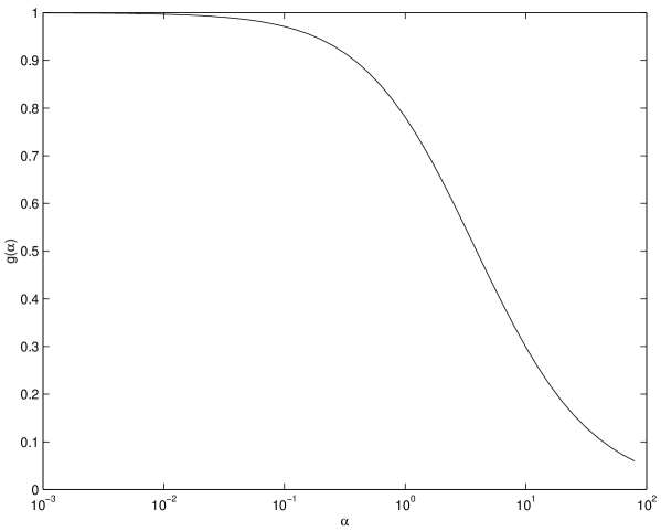
Figure 1: The phase-space suppression function ($\varepsilon=+1$ case)

3 The GZK sphere

In the sixties, Greisen [5], Zatsepin and Kuz’min [6] have shown that the cosmic microwave background radiation should make the Universe opaque to protons of energies $\gtrsim$ $10^{20}\,$eV. At these energies the thermal photons are sufficiently blue-shifted in the proton rest frame to excite baryon resonances and drain the proton’s energy via pion production. This led to the notion of GZK-sphere as being the sphere within which a source has to lie to supply us with protons at $10^{20}\,$eV. Later, more accurate calculations, using state-of-the-art particle physics data, placed the energy limit of cosmic (not arising from local sources) protons at around $5.10^{19}\,$eV. That is, if the proton sources are at cosmological distances ($\gtrsim$ $100$ Mpc), the observed spectrum should display a (GZK) cutoff around this energy. A similar limit applies to the nuclei component of the cosmic ray flux.

This situation was upset by the detection of a number of events above $10^{20}\,$eV without any plausible local sources [7] [8] [9]. Discrepancies between the fluxes measured by different groups [10] [11] and analysis of the combined data [12] do not yet allow for a clear-cut statement as to whether the GZK cutoff is indeed violated, a question that will hopefully be clarified by the forthcoming Auger observatory. Meanwhile a number of possible explanations for the violation of the GZK cutoff has appeared on the literature (for a review see [13]). Here I analyze the effect of the space-time non-commutativity on the calculation of the GZK cutoff and, when (and if) such cutoff is confirmed, what inferences can be taken concerning the value of $\ell$ and the sign $\epsilon$.

Simple letters are used to denote quantities in the lab (earth) frame, primed letters for the rest frame of the proton and starred letters for the center of mass. The fractional energy loss due to interactions with the cosmic background radiation (at zero redshift) is given by the integral of the nucleon energy loss per collision multiplied by the probability per unit time for a nucleon-photon collision in an isotropic gas of photons at temperature $T=2.7^{o}K$. Therefore the lifetime of a cosmic ray of energy $E$ is [14], $\left(\hbar=c=1\right)$

$$\tau_{0}\left(E\right)=2\Gamma^{2}\pi^{2}\left\{\sum_{j}\int_{\omega_{jth}^{{}^{\prime}}/2\Gamma}^{\infty}\frac{d\omega}{e^{\omega/kT}-1}\int_{\omega_{jth}^{{}^{\prime}}}^{2\Gamma\omega}d\omega^{{}^{\prime}}\omega^{{}^{\prime}}\sigma_{j}\left(\omega^{{}^{\prime}}\right)K_{j}\left(\omega^{{}^{\prime}}\right)\right\}^{-1}$$ (26)

where $\omega^{{}^{\prime}}$ is the photon energy in the nucleon rest frame and the inelasticity $K_{j}$ is the average energy lost by the photon for the channel $j$ with threshold $\omega_{jth}^{{}^{\prime}}$. $\sigma_{j}\left(\omega^{{}^{\prime}}\right)$ is the total cross section of the $j$-th interaction channel and $\Gamma$ the Lorentz factor of the nucleon $\left(\Gamma=\frac{E}{m_{p}}\right)$.

In (26) one may change the order of integration

$$\int_{\omega_{th}^{{}^{\prime}}/2\Gamma}^{\infty}d\omega\int_{\omega_{th}^{{}^{\prime}}}^{2\Gamma\omega}d\omega^{\prime}\rightarrow\int_{\omega_{th}^{{}^{\prime}}}^{\infty}d\omega^{\prime}\int_{\omega^{{}^{\prime}}/2\Gamma}^{\infty}d\omega$$

and compute one of the integrals.. To obtain the cosmic ray lifetime $\tau_{\ell}\left(E\right)$ in the non-commutative case, one multiplies the cross section by the suppression factor $g\left(\omega^{\prime},\epsilon\right)$ (Eq.(25)). Finally, changing variables

$$\omega^{\prime}\rightarrow y=e^{-\omega^{\prime}/\left(2\Gamma kT\right)}$$

one obtains the following ratio for each channel contribution

$$r_{g}=\frac{\tau_{\ell}\left(E\right)}{\tau_{0}\left(E\right)}=\frac{\int_{e^{\frac{\omega_{th}^{{}^{\prime}}}{\beta}}}^{0}\frac{dy}{y}\ln\left(1-y\right)\ln y\sigma\left(\beta\ln y\right)K\left(\beta\ln y\right)}{\int_{e^{\frac{\omega_{th}^{{}^{\prime}}}{\beta}}}^{0}\frac{dy}{y}\ln\left(1-y\right)\ln y\sigma\left(\beta\ln y\right)K\left(\beta\ln y\right)g\left(\beta^{2}\ell^{2}\ln^{2}y,\epsilon\right)}$$ (27)

with $\beta=-2\Gamma kT$.

This ratio was estimated for the single pion reaction (22) using $\omega_{th}^{\prime}=145$ MeV,

$$K\left(\omega^{\prime}\right)=\frac{1}{2}\left(1+\frac{m_{\pi}^{2}-m_{N}^{2}}{m_{p}^{2}+2m_{p}\omega^{\prime}}\right)$$

and the following parametrization [15] for the cross section

$$\sigma\left(\omega^{\prime}\right)=A+B\ln^{2}\left(\omega^{\prime}\right)+C\ln\left(\omega^{\prime}\right)$$

with $A=0.147,B=0.0022,C=-0.017$ , $\omega^{\prime}$ in Gev’s. This is a parametrization for the $\gamma p$ total cross section in the range $3$GeV$<\omega^{\prime}<183$GeV. Of course, to compute the absolute value of $\tau_{\ell}\left(E\right)$ this would not be appropriate. Instead, due account should be taken of all the resonances contributions. However for the ratio $r_{g}$ it gives, at least, qualitative information on the order of magnitude of the effect.

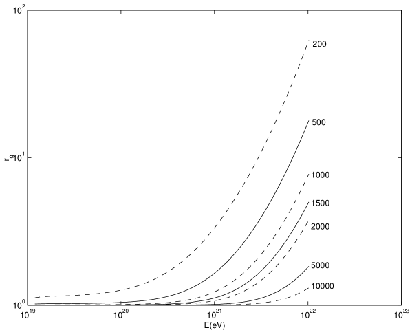
Figure 2: Cosmic ray lifetime increasing factors for $1/\ell$ in the range $200$ to $10000$ MeV ($\varepsilon=+1$ case)

In Fig.2 the results for $r_{g}$ are shown for $\epsilon=+1$ and $1/\ell$ in the range $200$ to $10000$ Mev, that is, $\ell$ in the range $0.98-0.0197$ Fermi or $329-6.58\times 10^{-26}$ seconds.

To estimate the effect that this lifetime extending factors have on the energy attenuation of cosmic rays on route to earth, I have used the $\left(dD/dE\right)_{\infty}$ values found in [16] for a $10^{22}$ eV nucleon and computed the integration

$$D\left(E\right)=D_{0}\left(E_{0}\right)+\int_{E_{0}}^{E}r_{g}\left(E\right)\left(dD/dE\right)_{\infty}dE$$ (28)

The results are shown in Fig. 3. One sees that whereas the value of the GZK cutoff is not much changed, the radius of the GZK sphere is increased allowing for nucleons from distances beyond $100$ Mpc to reach earth at energies above $5.10^{19}$ eV.

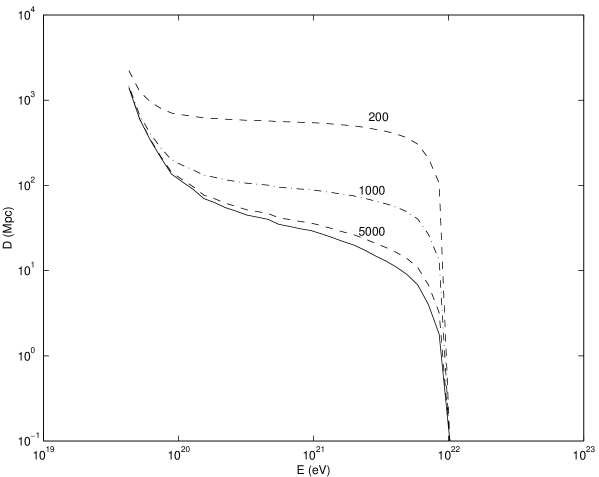
Figure 3: Energy attenuation of a $10^{22}$ eV nucleon in route to earth: $1/\ell=200,1000,5000$ MeV compared with the $\ell=0$ case

If the observation of the ultra high energy cosmic rays is indeed a manifestation of the non-commutative structure two conclusions may be taken:

- First, that the sign $\epsilon$ is $+1$, that is, space is continuous and time discrete.

- Second, that for the effect to be significant at current cosmic ray energies, the time quantum must be $\gtrsim 10^{-25}$ seconds, much larger than Planck scale times.

4 Corrections to the spectrum of the Coulomb problem

Some experiments in atomic physics are now sensitive to small frequency shifts below 1 mHz. With such sensitivity, non-commutative space-time effects might be detected at low energies, especially if small energy shifts have a qualitative impact. Here such a possibility is analyzed by looking at the effect of the non-commutative algebra on the spectrum of the Coulomb problem. Consider the Hamiltonian

$$H=-\frac{1}{2m}\Delta-\frac{e^{2}}{\left|\overrightarrow{x}\right|}$$ (29)

and use, for the non-commutative coordinates and momenta, the representation listed in the Appendix. Both cases ($\epsilon=-1$ and $\epsilon=+1$) will be considered.

$\epsilon=-1$

From (42) one obtains (setting $R=1$)

$$\begin{array}[]{lll}\left|\overrightarrow{p}\right|^{2}&=&\frac{1}{\ell^{2}}\sin^{2}\theta_{3}\\ \left|\overrightarrow{x}\right|^{2}&=&\ell^{2}\left\{L^{2}\cot^{2}\theta_{3}-\frac{\partial^{2}}{\partial\theta_{3}^{2}}-2\cot\theta_{3}\frac{\partial}{\partial\theta_{3}}\right\}\end{array}$$ (30)

Therefore

$$H=\frac{1}{2m\ell^{2}}\sin^{2}\theta_{3}-\frac{e^{2}}{\ell}\left\{L^{2}\cot^{2}\theta_{3}-\frac{\partial^{2}}{\partial\theta_{3}^{2}}-2\cot\theta_{3}\frac{\partial}{\partial\theta_{3}}\right\}^{-\frac{1}{2}}$$ (31)

For small $\ell$, (small $\theta_{3}$) one obtains

$$H\simeq\frac{1}{2m}\left\{\frac{\theta_{3}^{2}}{\ell^{2}}-\frac{\ell^{2}}{3}\left(\frac{\theta_{3}}{\ell}\right)^{4}\right\}-e^{2}\left\{L^{2}\left(\frac{\ell^{2}}{\theta_{3}^{2}}-\frac{2\ell^{2}}{3}\right)-\ell^{2}\frac{\partial^{2}}{\partial\theta_{3}^{2}}-2\ell^{2}\left(\frac{1}{\theta_{3}}-\frac{\theta_{3}}{3}\right)\frac{\partial}{\partial\theta_{3}}\right\}^{-\frac{1}{2}}$$ (32)

In this approximation $p\simeq\frac{\theta_{3}}{\ell}$, therefore

$$H\simeq\frac{1}{2m}\left\{p^{2}-\frac{\ell^{2}}{3}p^{4}\right\}-e^{2}\left\{L^{2}\left(\frac{1}{p^{2}}-\frac{2\ell^{2}}{3}\right)-\frac{\partial^{2}}{\partial p^{2}}-2\left(\frac{1}{p}-\frac{\ell^{2}}{3}p\right)\frac{\partial}{\partial p}\right\}^{-\frac{1}{2}}$$

which may be rewritten

$$H\simeq\frac{1}{2m}p^{2}-\frac{e^{2}}{\left(\nabla_{p}^{2}\right)^{\frac{1}{2}}}+\ell^{2}\left\{-\frac{1}{6m}p^{4}-\frac{e^{2}\left(L^{2}-p\frac{\partial}{\partial p}\right)}{3\left(\nabla_{p}^{2}\right)^{\frac{3}{2}}}\right\}$$ (33)

with $\nabla_{p}^{2}=\frac{L^{2}}{p^{2}}-\frac{\partial^{2}}{\partial p^{2}}-\frac{2}{p}\frac{\partial}{\partial p}$

Using the Fourier transform $f\left(x\right)=\int e^{ip.x}F\left(p\right)d^{3}p$ and the relations

$$\begin{array}[]{lll}\int e^{ip.x}p^{2}F\left(p\right)d^{3}p&=&-\nabla_{x}^{2}f\left(x\right)\\ \int e^{ip.x}\nabla_{p}^{2}F\left(p\right)d^{3}p&=&-x^{2}f\left(x\right)\\ \int e^{ip.x}p\frac{\partial}{\partial p}F\left(p\right)d^{3}p&=&\left(-r\frac{\partial}{\partial r}-3\right)f\left(x\right)\end{array}$$ (34)

one obtains a configuration space representation of Eq.(33), namely

$$H\simeq-\frac{\nabla_{x}^{2}}{2m}-\frac{e^{2}}{\left|x\right|}-\ell^{2}\left\{\frac{1}{6m}\nabla_{x}^{4}+\frac{e^{2}}{3}\frac{L^{2}+r\frac{\partial}{\partial r}+3}{r^{3}}\right\}$$ (35)

The first two terms are the usual Coulomb Hamiltonian and the third is the order $\ell^{2}$ correction arising from the non-commutative structure.

$$\left\langle n^{\prime}L^{{}^{\prime}}M^{{}^{\prime}}\left|H\right|nLM\right\rangle\simeq\delta_{LL^{{}^{\prime}}}\delta_{MM^{{}^{\prime}}}\left\{E_{n}\delta_{n^{\prime},n}+\ell^{2}\left\langle-\frac{1}{6m}\nabla_{x}^{4}-\frac{e^{2}}{3}\frac{L\left(L+1\right)+r\frac{\partial}{\partial r}+3}{r^{3}}\right\rangle_{n^{\prime},n}\right\}$$ (36)

where $r=\left|\overrightarrow{x}\right|$.

$\epsilon=+1$

For the $\epsilon=+1$ case one uses the same representation with the replacements $x^{\nu}\rightarrow ix^{\nu},p^{\nu}\rightarrow-ip^{\nu},\theta_{3}\rightarrow i\mu$, to obtain

$$\begin{array}[]{lll}\left|\overrightarrow{p}\right|^{2}&=&\frac{1}{\ell^{2}}\sinh^{2}\mu\\ \left|\overrightarrow{x}\right|^{2}&=&\ell^{2}\left\{L^{2}\coth^{2}\mu-\frac{\partial^{2}}{\partial\mu^{2}}-2\coth\mu\frac{\partial}{\partial\mu}\right\}\end{array}$$ (37)

Then

$$H=\frac{1}{2m\ell^{2}}\sinh^{2}\mu-\frac{e^{2}}{\ell}\left\{L^{2}\coth^{2}\mu-\frac{\partial^{2}}{\partial\mu^{2}}-2\coth\mu\frac{\partial}{\partial\mu}\right\}^{-\frac{1}{2}}$$ (38)

and for small $\mu$

$$H\simeq\frac{1}{2m}\left\{\frac{\mu^{2}}{\ell^{2}}+\frac{\ell^{2}}{3}\left(\frac{\mu}{\ell}\right)^{4}\right\}-e^{2}\left\{L^{2}\left(\frac{\ell^{2}}{\mu^{2}}+\frac{2\ell^{2}}{3}\right)-\ell^{2}\frac{\partial^{2}}{\partial\mu^{2}}-2\ell^{2}\left(\frac{1}{\mu}+\frac{\mu}{3}\right)\frac{\partial}{\partial\mu}\right\}^{-\frac{1}{2}}$$

$$H\simeq\frac{1}{2m}\left\{p^{2}+\frac{\ell^{2}}{3}p^{4}\right\}-e^{2}\left\{L^{2}\left(\frac{1}{p^{2}}+\frac{2\ell^{2}}{3}\right)-\frac{\partial^{2}}{\partial p^{2}}-2\left(\frac{1}{p}+\frac{\ell^{2}}{3}p\right)\frac{\partial}{\partial p}\right\}^{-\frac{1}{2}}$$

$$H\simeq\frac{1}{2m}p^{2}-\frac{e^{2}}{\left(\nabla_{p}^{2}\right)^{\frac{1}{2}}}+\ell^{2}\left\{\frac{1}{6m}p^{4}+\frac{e^{2}\left(L^{2}-p\frac{\partial}{\partial p}\right)}{3\left(\nabla_{p}^{2}\right)^{\frac{3}{2}}}\right\}$$

$$H\simeq-\frac{\nabla_{x}^{2}}{2m}-\frac{e^{2}}{\left|x\right|}+\ell^{2}\left\{\frac{1}{6m}\nabla_{x}^{4}+\frac{e^{2}}{3}\frac{L^{2}+r\frac{\partial}{\partial r}+3}{r^{3}}\right\}$$ (39)

the conclusion being that for the $\epsilon=+1$ case the order $\ell^{2}$ correction differs from the $\epsilon=-1$ case by a sign change.

5 Conclusions

1) A non-commutative space-time structure and two constants of Nature $\ell$ and $\epsilon$ emerge as natural consequences of deformation-theory and stability of the fundamental physical theories. Among other effects, this structure implies a modification of phase-space volume which, in particular, has a bearing on the calculation of the GZK sphere. Lorentz invariance is preserved.

2) Phase-space suppression effects occur only in the $\epsilon=+1$ case. In this case the time coordinate has a discrete spectrum and space coordinates are continuous.

3) In addition to changing the cross sections of elementary processes, phase-space counting rules have statistical mechanics consequences which might have had a relevant effect at the first stages of the Universe evolution.

4) Phase-space volume modifications, time and space coordinates spectra and modifications of the uncertainty relations are consequences of the non-commutative space-time structure which depend only on its algebraic structure. In this sense they are very robust and provide unambiguous tests of the theory. Other consequences might depend on the particular geometric construction that is built on top of the algebraic structure. For example, for a particular geometrical construction [3] the existence of additional components on gauge fields is an intriguing consequence.

Appendix A

For specific calculations it is convenient to use a representation of the space-time algebra ($\varepsilon=-1$ case) in the space of functions on the upper sheet of the cone $C^{4}$, with coordinates

$$\begin{array}[]{lll}\xi_{1}&=&R\sin\theta_{3}\sin\theta_{2}\sin\theta_{1}\\ \xi_{2}&=&R\sin\theta_{3}\sin\theta_{2}\cos\theta_{1}\\ \xi_{3}&=&R\sin\theta_{3}\cos\theta_{2}\\ \xi_{4}&=&R\cos\theta_{3}\\ \xi_{5}&=&R\end{array}$$ (40)

the invariant measure for which the functions are square-integrable being

$$d\nu(R,\theta_{i})=R^{2}\sin^{2}\theta_{3}\sin\theta_{2}dRd\theta_{1}d\theta_{2}d\theta_{3}$$ (41)

On these functions the operators of $\Re_{\ell,\infty}$ act as follows

$$\begin{array}[]{lll}\ell p^{0}&=&R\\ \Im&=&R\cos\theta_{3}\\ \ell p^{1}&=&R\sin\theta_{3}\cos\theta_{2}\\ \ell p^{2}&=&R\sin\theta_{3}\sin\theta_{2}\cos\theta_{1}\\ \ell p^{3}&=&R\sin\theta_{3}\sin\theta_{2}\sin\theta_{1}\\ M^{23}&=&-i\frac{\partial}{\partial\theta_{1}}\\ M^{12}&=&-i\left(\cos\theta_{1}\frac{\partial}{\partial\theta_{2}}-\sin\theta_{1}\cot\theta_{2}\frac{\partial}{\partial\theta_{1}}\right)\\ M^{31}&=&i\left(\sin\theta_{1}\frac{\partial}{\partial\theta_{2}}+\cos\theta_{1}\cot\theta_{2}\frac{\partial}{\partial\theta_{1}}\right)\\ \frac{x^{0}}{\ell}&=&-i\left(-\sin\theta_{3}\frac{\partial}{\partial\theta_{3}}+R\cos\theta_{3}\frac{\partial}{\partial R}\right)\\ \frac{x^{1}}{\ell}&=&i\left(\cos\theta_{2}\frac{\partial}{\partial\theta_{3}}-\sin\theta_{2}\cot\theta_{3}\frac{\partial}{\partial\theta_{2}}\right)\\ \frac{x^{2}}{\ell}&=&i\left(\cos\theta_{1}\sin\theta_{2}\frac{\partial}{\partial\theta_{3}}+\cos\theta_{1}\cos\theta_{2}\cot\theta_{3}\frac{\partial}{\partial\theta_{2}}-\frac{\sin\theta_{1}}{\sin\theta_{2}}\cot\theta_{3}\frac{\partial}{\partial\theta_{1}}\right)\\ \frac{x^{3}}{\ell}&=&i\left(\sin\theta_{1}\sin\theta_{2}\frac{\partial}{\partial\theta_{3}}+\sin\theta_{1}\cos\theta_{2}\cot\theta_{3}\frac{\partial}{\partial\theta_{2}}+\frac{\cos\theta_{1}}{\sin\theta_{2}}\cot\theta_{3}\frac{\partial}{\partial\theta_{1}}\right)\\ M^{01}&=&i\left(\frac{\sin\theta_{2}}{\sin\theta_{3}}\frac{\partial}{\partial\theta_{2}}-\cos\theta_{2}\cos\theta_{3}\frac{\partial}{\partial\theta_{3}}-R\cos\theta_{2}\sin\theta_{3}\frac{\partial}{\partial R}\right)\\ M^{02}&=&-i\left(\begin{array}[]{c}\frac{\cos\theta_{1}\cos\theta_{2}}{\sin\theta_{3}}\frac{\partial}{\partial\theta_{2}}-\frac{\sin\theta_{1}}{\sin\theta_{2}\sin\theta_{3}}\frac{\partial}{\partial\theta_{1}}+\cos\theta_{1}\sin\theta_{2}\cos\theta_{3}\frac{\partial}{\partial\theta_{3}}+\\ R\cos\theta_{1}\sin\theta_{2}\sin\theta_{3}\frac{\partial}{\partial R}\end{array}\right)\\ M^{03}&=&-i\left(\begin{array}[]{c}\frac{\sin\theta_{1}\cos\theta_{2}}{\sin\theta_{3}}\frac{\partial}{\partial\theta_{2}}+\frac{\cos\theta_{1}}{\sin\theta_{2}\sin\theta_{3}}\frac{\partial}{\partial\theta_{1}}+\sin\theta_{1}\sin\theta_{2}\cos\theta_{3}\frac{\partial}{\partial\theta_{3}}+\\ R\sin\theta_{1}\sin\theta_{2}\sin\theta_{3}\frac{\partial}{\partial R}\end{array}\right)\end{array}$$ (42)

For the $\varepsilon=+1$ case, one may work out a similar representation on the $C^{3,1}$ cone with coordinates

$$\begin{array}[]{lll}\zeta_{1}&=&R\cosh\beta\cos\psi_{0}\\ \zeta_{2}&=&R\cosh\beta\sin\psi_{0}\\ \zeta_{3}&=&R\sinh\beta\sin\psi_{1}\\ \zeta_{4}&=&R\sinh\beta\cos\psi_{1}\\ \zeta_{5}&=&R\end{array}$$ (43)

Alternatively we may use the above representation multiplying $x^{\mu}$ by $i$, $p^{\mu}$ by $-i$ and replacing $\theta_{3}$ by $i\mu$. It is easily seen from (1) that the correct commutation relations, for the $\varepsilon=+1$ case, are obtained.

References

[1] R. Vilela Mendes; J. Phys. A: Math. Gen. 27 (1994) 8091.
[2] R. Vilela Mendes; Phys. Lett. A210 (1996) 232.
[3] R. Vilela Mendes; J. Math. Phys. 41 (2000) 156.
[4] E. Carlen and R. Vilela Mendes; Phys. Lett. A 290 (2001) 109.
[5] K. Greisen; Phys. Rev. Lett. 16 (1966) 748.
[6] G. T. Zatsepin and V. A. Kuz’min; JETP Lett. 4 (1966) 78.
[7] D. J. Bird et al.;Astrophys. J. 441 (1995) 144.
[8] M. Takeda et al.;Phys. Rev. Lett. 81 (1998) 1163.
[9] M. Takeda et al.; Astropart. Phys. 19 (2003) 447.
[10] T. Abu-Zayyad et al.; arXiv:astro-ph/0208243.
[11] T. Abu-Zayyad et al.; arXiv:astro-ph/0208301.
[12] J. N. Bahcall and E. Waxman; Phys. Lett. B556 (2003) 1.
[13] L. Anchordoqui, T. Paul, S. Reucroft and J. Swain;
Int. J. Mod. Phys. A18 (2003) 2229.
[14] F. W. Stecker; Phys. Rev. Lett. 21 (1968) 1016.
[15] L. Montanet et al.; Phys. Rev. D 50 (1994) 1173.
[16] L. Anchordoqui, M. T. Dova, L. N. Epele and J. D.
Swain; Phys. Rev. D 55 (1997) 7356.