The Gluon Green’s Function in N = 4 Supersymmetric Yang–Mills Theory

Abstract

The high energy limit of scattering amplitudes in the N = 4 supersymmetric Yang–Mills theory is studied by solving the corresponding BFKL equation in the next–to–leading approximation. The gluon Green’s function is analysed using a newly proposed method suitable for investigating the contribution from higher conformal spins. From this new approach complete agreement is obtained with the results of Kotikov and Lipatov on conformal spins and angular dependence.

,

1 Introduction

In recent years there has been a large interest in the study of the next–to–leading (NLL) corrections to the Balitsky–Fadin–Kuraev–Lipatov [1] (BFKL) equation in QCD [2, 3, 4, 5]. The calculation of the NLL corrections was extended to supersymmetric gauge theories in Ref. [6]. In that work it was shown how in a N = 4 SYM theoretical playground the kernel of the BFKL equation is simplified. In particular, the analyticity of the eigenvalues in terms of the conformal spins allowed the study of the connection between the DGLAP and BFKL equations in this model, this being possible mainly due to the lack of coupling constant renormalisation. In Ref. [7] the anomalous dimension matrix of the Wilson twist–2 operators in this maximally supersymmetric theory in four dimensions was calculated at two loops. Very recently these results were extended to three loops in Ref. [8] using the calculation for the non–singlet case first obtained in Ref. [9], and in agreement, in the supersymmetric limit, with the results for the singlet case derived in Ref. [10].

In the present study, the method for solving the BFKL equation at NLL accuracy developed in Ref. [14, 15] is applied to N = 4 SYM. This will serve two purposes. Firstly, since the method solves the BFKL equation with full angular information, it can be used to test the results in the literature [6] for the dependence of the eigenvalues of the kernel on conformal spins. Secondly, due to the conformal invariance of the theory also at higher orders, the analytic solution to the NLL BFKL equation is known for N = 4 SYM, and therefore it is possible to directly test the results obtained using the completely independent method described in this work. The results in the literature for the solution of the N = 4 SYM BFKL equation at NLL in terms of conformal eigenfunctions are reviewed in the next section. In Sec. 3 the NLL BFKL equation is solved directly in momentum space using the iterative method of Ref.[14, 15]. Sec. 4 is devoted to a study of the numerical structure of the trajectory and the real emission kernel arising in this approach. In Sec. 5 the results obtained in the two approaches are compared and the conclusions are presented.

2 The BFKL equation and its solution in Mellin space

In the BFKL formalism the high energy limit of a scattering process factorizes as

$$\sigma(s) = \int\frac{d^{2}\vec{k}_{a}}{\vec{k}_{a}^{2}}\int\frac{d^{2}\vec{k}_{b}}{\vec{k}_{b}^{2}}~{}\Phi(\vec{k}_{a})~{}\Phi^{\prime}(\vec{k}_{b})~{}f\left(\vec{k}_{a},\vec{k}_{b},{\rm Y}\equiv\ln{\frac{s}{s_{0}}}\right),$$ (1)

where $s_{0}=|\vec{k}_{a}||\vec{k}_{b}|$ is the Regge scale. The energy dependence is determined by the universal process–independent gluon Green’s function $f$. The impact factors, $\Phi,\Phi^{\prime}$, depend on the process under study. In the Regge–limit of large centre of mass energy and fixed momentum transfer the effective degrees of freedom are the transverse momenta $\vec{k}_{a,b}$ of the exchanged gluons. The dynamics of these processes is then two–dimensional evolving with a time variable Y. The evolution of the gluon Green’s function with Y is governed by the BFKL equation. This equation is traditionally written in terms of a Mellin transform of Y, i.e.

$$f\left(\vec{k}_{a},\vec{k}_{b},{\rm Y}\right) = \frac{1}{2\pi i}\int_{a-i\infty}^{a+i\infty}d\omega~{}e^{\omega{\rm Y}}f_{\omega}\left(\vec{k}_{a},\vec{k}_{b}\right).$$ (2)

With such transformation the equation reads

$$\omega f_{\omega}\left(\vec{k}_{a},\vec{k}_{b}\right) = \delta^{(2)}\left(\vec{k}_{a}-\vec{k}_{b}\right)+\int d^{2}\vec{k}^{\prime}~{}\mathcal{K}\left(\vec{k}_{a},\vec{k}^{\prime}\right)f_{\omega}\left(\vec{k}^{\prime},\vec{k}_{b}\right).$$ (3)

The inhomogeneous term of this integral equation corresponds to a single gluon exchange and the kernel (in dimensional regularization, $D=4+2\epsilon$)

$$\mathcal{K}\left(\vec{k}_{a},\vec{k}\right)=2\,\omega^{(\epsilon)}\left(\vec{k}_{a}^{2}\right)\,\delta^{(2+2\epsilon)}\left(\vec{k}_{a}-\vec{k}\right)+\mathcal{K}_{r}\left(\vec{k}_{a},\vec{k}\right)$$ (4)

contains the gluon Regge trajectory [6],

$$2\,\omega^{(\epsilon)}\left(\vec{q}^{2}\right) = -a\left(\frac{1}{\epsilon}+\ln{\frac{\vec{q}^{2}}{\mu^{2}}}\right)$$ (5)

$$-\frac{a^{2}}{8}\left[\left(\frac{1}{3}-2\zeta(2)\right)\left(\frac{1}{\epsilon}+2\ln{\frac{\vec{q}^{2}}{\mu^{2}}}\right)-\frac{8}{9}+2\zeta(3)\right],$$

with the coupling $a=\frac{{\overline{g}}^{2}N_{c}}{4\pi^{2}}$, which is not running in N = 4 SYM. The kernel also includes two contributions from the real emissions:

$$\mathcal{K}_{r} = {\mathcal{K}}_{r}^{(\epsilon)}+\widetilde{\mathcal{K}}_{r}$$ (6)

where [6]

$$\mathcal{K}_{r}^{(\epsilon)}\left(\vec{q},\vec{q}+\vec{k}\right) = \frac{a\,\mu^{-2\epsilon}}{\pi^{1+\epsilon}\Gamma(1-\epsilon)}\frac{1}{\vec{k}^{2}}$$ (7)

$$\times \left\{1+\frac{a}{4}\left(\frac{\vec{k}^{2}}{\mu^{2}}\right)^{\epsilon}\left[\frac{1}{3}-2\,\zeta(2)+\epsilon\left(-\frac{8}{9}+14\,\zeta(3)\right)\right]\right\}$$

and [6]

$$\widetilde{\mathcal{K}}_{r}\left(\vec{q},\vec{p}\right) = \frac{a^{2}}{4\pi}\left\{-\frac{1}{(\vec{q}-\vec{p})^{2}}\ln^{2}{\frac{\vec{q}^{2}}{\vec{p}^{2}}}\right.$$ (8)

$$+\frac{2(\vec{q}^{2}-{\vec{p}}^{2})}{(\vec{q}-{\vec{p}})^{2}(\vec{q}+{\vec{p}})^{2}}\left(\frac{1}{2}\ln{\frac{\vec{q}^{2}}{{\vec{p}}^{2}}}\ln{\frac{\vec{q}^{2}{\vec{p}}^{2}(\vec{q}-{\vec{p}})^{4}}{(\vec{q}^{2}+{\vec{p}}^{2})^{4}}}+\left(\int_{0}^{-\frac{\vec{q}^{2}}{{\vec{p}}^{2}}}-\int_{0}^{-\frac{{\vec{p}}^{2}}{\vec{q}^{2}}}\right)dt\frac{\ln(1-t)}{t}\right)$$

$$\left.-\left(1-\frac{(\vec{q}^{2}-{\vec{p}}^{2})^{2}}{(\vec{q}-{\vec{p}})^{2}(\vec{q}+{\vec{p}})^{2}}\right)\left(\left(\int_{0}^{1}-\int_{1}^{\infty}\right)dz\frac{1}{({\vec{p}}-z\vec{q})^{2}}\ln{\frac{(z\vec{q})^{2}}{{\vec{p}}^{2}}}\right)\right\}.$$

In N = 4 SYM the BFKL kernel respects conformal symmetry even at NLL accuracy, and the eigenfunctions do not change compared to the leading logarithmic (LL) ones. The solution to this equation can therefore be found using the expansion on the known eigenfunctions

$$f\left(\vec{k}_{a},\vec{k}_{b},Y\right) = \frac{1}{\pi|\vec{k}_{a}||\vec{k}_{b}|}\sum_{n=-\infty}^{\infty}\int\frac{d\omega}{2\pi i}\,e^{\omega Y}\int\frac{d\gamma}{2\pi i}\left(\frac{\vec{k}_{a}^{2}}{\vec{k}_{b}^{2}}\right)^{\gamma-\frac{1}{2}}\frac{e^{in\theta}}{\omega-\omega_{n}(a,\gamma)},$$ (9)

with $\theta$ the angle defined by the $\vec{k}_{a}$ and $\vec{k}_{b}$ transverse momenta. The Fourier transform in angles is characterized by the so–called conformal spins $n$. Given that the coupling is fixed it is possible to fully diagonalize the BFKL kernel by simply acting on the LL eigenfunctions, i.e., in the $\overline{\rm MS}$ scheme we have [6]

$$\int d^{2}\vec{q}\,\mathcal{K}\left(\vec{k},\vec{q}\right)\left(\frac{\vec{q}^{2}}{\vec{k}^{2}}\right)^{\gamma-1}e^{in\theta} = \omega_{n}(a,\gamma)=\xi^{\rm MS}\chi(|n|,\gamma)+\eta+\Omega(|n|,\gamma).$$ (10)

In this expression we have defined

$$\xi^{\rm MS} \equiv a+a^{2}\left(\frac{1}{12}-\frac{\zeta(2)}{2}\right)\,,\,\,\,\eta~{}\equiv~{}a^{2}\,\frac{3}{2}\,\zeta(3)$$ (11)

and

$$\chi(n,\gamma) = 2\Psi(1)-\Psi\left(\gamma+\frac{n}{2}\right)-\Psi\left(1-\gamma+\frac{n}{2}\right),$$ (13)

$$\Omega(n,\gamma)~{}=~{}\frac{a^{2}}{4}\left[\Psi^{\prime\prime}\left(\gamma+\frac{n}{2}\right)+\Psi^{\prime\prime}\left(1-\gamma+\frac{n}{2}\right)-2\Phi(n,\gamma)-2\Phi(n,1-\gamma)\right]$$

$$\Phi(n,\gamma) = \sum_{k=0}^{\infty}\frac{(-1)^{(k+1)}}{k+\gamma+\frac{n}{2}}\left[\frac{}{}\Psi^{\prime}(k+n+1)-\Psi^{\prime}(k+1)\right.$$ (14)

$$\hskip 56.9055pt+(-1)^{(k+1)}\left(\beta^{\prime}(k+n+1)+\beta^{\prime}(k+1)\right)$$

$$\hskip 56.9055pt-\left.\frac{1}{k+\gamma+\frac{n}{2}}\left(\Psi(k+n+1)-\Psi(k+1)\right)\right],$$

$$\beta^{\prime}(z) = \frac{1}{4}\left[\Psi^{\prime}\left(\frac{1+z}{2}\right)-\Psi^{\prime}\left(\frac{z}{2}\right)\right].$$ (15)

We have checked that switching to the gluon–bremsstrahlung (GB) scheme

$$a_{\rm GB} = a+\left(\frac{1}{12}-\frac{\zeta(2)}{2}\right)a^{2},\,\,\,\,\,\xi^{\rm GB}~{}=~{}a_{\rm GB},$$ (16)

or to the dimensional reduction (DRED) scheme, which respects SUSY [6],

$$a_{\rm DRED} = a+\frac{1}{12}a^{2},\,\,\,\,\,\xi^{\rm DRED}~{}=~{}a_{\rm DRED}-\frac{\zeta(2)}{2}{a_{\rm DRED}}^{2},$$ (17)

the results of this work do not change qualitatively.

The analyticity of these expressions, obtained by Kotikov and Lipatov in [6], for the dependence of the eigenvalues of the NLL BFKL kernel on the conformal spins is very important. It allows the analytic continuation to negative $|n|$ and to find the connection between the BFKL equation and DGLAP in the N = 4 supersymmetric gauge theory. One of the objectives of the present work will be to confirm that these results for the conformal spins are correct using a completely orthogonal method of solution of the BFKL equation, which is developed in the next section.

3 The solution directly in transverse–momentum space

The starting point of the new method of solution is Eq. (3) with the infrared divergences regularized in dimensional regularization. In the real emission kernel there are contributions which will lead to $\epsilon$ poles after phase space integration, $\mathcal{K}_{r}^{(\epsilon)}$, and others which will be finite, $\mathcal{K}_{r}$, i.e.

$$\omega f_{\omega}\left(\vec{k}_{a},\vec{k}_{b}\right) = \delta^{(2+2\epsilon)}\left(\vec{k}_{a}-\vec{k}_{b}\right)$$ (18)

$$+ \int d^{2+2\epsilon}\vec{k}\,2\,\omega^{(\epsilon)}\left(\vec{k}_{a}^{2}\right)\delta^{(2+2\epsilon)}\left(\vec{k}_{a}-\vec{k}\right)f_{\omega}\left(\vec{k},\vec{k}_{b}\right)$$

$$+ \int d^{2+2\epsilon}\vec{k}\,\mathcal{K}_{r}^{(\epsilon)}\left(\vec{k}_{a},\vec{k}_{a}+\vec{k}\right)f_{\omega}\left(\vec{k}_{a}+\vec{k},\vec{k}_{b}\right)$$

$$+ \int d^{2+2\epsilon}\vec{k}\,\widetilde{\mathcal{K}}_{r}\left(\vec{k}_{a},\vec{k}_{a}+\vec{k}\right)f_{\omega}\left(\vec{k}_{a}+\vec{k},\vec{k}_{b}\right).$$

In order to explicitly show the cancellation of the infrared $\epsilon$ divergencies we introduce a phase space slicing parameter, $\lambda$, in the integral over real emission, and make use of the approximation

$$f_{\omega}\left(\vec{k}+\vec{k}_{a},\vec{k}_{b}\right) \simeq f_{\omega}\left(\vec{k}+\vec{k}_{a},\vec{k}_{b}\right)\theta\left(\vec{k}^{2}-\lambda^{2}\right)+f_{\omega}\left(\vec{k}_{a},\vec{k}_{b}\right)\theta\left(\lambda^{2}-\vec{k}^{2}\right).$$ (19)

This is valid when $\lambda$ is small compared to $k_{a}$. Hence the equation now reads

$$\omega f_{\omega}\left(\vec{k}_{a},\vec{k}_{b}\right) = \delta^{(2+2\epsilon)}\left(\vec{k}_{a}-\vec{k}_{b}\right)$$

$$+\left\{2\,\omega^{(\epsilon)}\left(\vec{k}_{a}^{2}\right)+\int d^{2+2\epsilon}\vec{k}\,\mathcal{K}_{r}^{(\epsilon)}\left(\vec{k}_{a},\vec{k}_{a}+\vec{k}\right)\theta\left(\lambda^{2}-\vec{k}^{2}\right)\right\}f_{\omega}\left(\vec{k}_{a},\vec{k}_{b}\right)$$

$$+\int d^{2+2\epsilon}\vec{k}\,\left\{\mathcal{K}_{r}^{(\epsilon)}\left(\vec{k}_{a},\vec{k}_{a}+\vec{k}\right)\theta\left(\vec{k}^{2}-\lambda^{2}\right)+\widetilde{\mathcal{K}}_{r}\left(\vec{k}_{a},\vec{k}_{a}+\vec{k}\right)\right\}f_{\omega}\left(\vec{k}_{a}+\vec{k},\vec{k}_{b}\right).$$

We have performed the integration over phase space for those emissions below the infrared cut–off $\lambda$, obtaining the result

$$\int d^{2+2\epsilon}\vec{k}\,\mathcal{K}_{r}^{(\epsilon)}\left(\vec{q},\vec{q}+\vec{k}\right)\theta\left(\lambda^{2}-\vec{k}^{2}\right) = \frac{a}{\Gamma(1+\epsilon)\Gamma(1-\epsilon)}\frac{1}{\epsilon}\left(\frac{\lambda^{2}}{\mu^{2}}\right)^{\epsilon}$$ (21)

$$\times\left\{1+\frac{a}{8}\left(\frac{\lambda^{2}}{\mu^{2}}\right)^{\epsilon}\left[\frac{1}{3}-2\,\zeta(2)+\epsilon\left(-\frac{8}{9}+14\,\zeta(3)\right)\right]\right\}.$$

Now it is possible to show how the poles cancel by calculating the gluon Regge trajectory in our regularisation scheme, i.e.

$$\omega_{0}\left({\vec{q}}^{2},\lambda\right) \equiv \lim_{\epsilon\to 0}\left\{2\,\omega^{(\epsilon)}\left(\vec{q}^{2}\right)+\int d^{2+2\epsilon}\vec{k}\,\mathcal{K}_{r}^{(\epsilon)}\left(\vec{q},\vec{q}+\vec{k}\right)\theta\left(\lambda^{2}-\vec{k}^{2}\right)\right\}$$ (22)

$$= -a\left\{\ln{\frac{\vec{q}^{2}}{\lambda^{2}}}+\frac{a}{4}\left[\left(\frac{1}{3}-2\xi(2)\right)\ln{\frac{\vec{q}^{2}}{\lambda^{2}}}-6\,\zeta(3)\right]\right\}$$

$$\equiv -\xi^{\rm MS}\ln{\frac{\vec{q}^{2}}{\lambda^{2}}}+\eta,$$

where $\xi$ and $\eta$ coincide with those defined in Eq. (11). The corresponding real emission part will be of the form

$$\lim_{\epsilon\to 0}\int d^{2+2\epsilon}\vec{k}\,\mathcal{K}_{r}^{(\epsilon)}\left(\vec{k}_{a},\vec{k}_{a}+\vec{k}\right)\theta\left(\vec{k}^{2}-\lambda^{2}\right)f_{\omega}\left(\vec{k}_{a}+\vec{k},\vec{k}_{b}\right) =$$ (23)

$$\int d^{2}\vec{k}\,\frac{1}{\pi\vec{k}^{2}}\,\xi^{\rm MS}\,\theta\left(\vec{k}^{2}-\lambda^{2}\right)f_{\omega}\left(\vec{k}_{a}+\vec{k},\vec{k}_{b}\right).$$

Finally the N=4 SYM NLL BFKL equation can be expressed as

$$\left(\omega-\omega_{0}\left(\vec{k}_{a}^{2},\lambda^{2}\right)\right)f_{\omega}\left(\vec{k}_{a},\vec{k}_{b}\right) = \delta^{(2)}\left(\vec{k}_{a}-\vec{k}_{b}\right)$$ (24)

$$+\int d^{2}\vec{k}\left(\frac{1}{\pi\vec{k}^{2}}\,\xi^{\rm MS}\,\theta\left(\vec{k}^{2}-\lambda^{2}\right)+\widetilde{\mathcal{K}}_{r}\left(\vec{k}_{a},\vec{k}_{a}+\vec{k}\right)\right)f_{\omega}\left(\vec{k}_{a}+\vec{k},\vec{k}_{b}\right).$$

Note that the treatment of the kernel is with its full angular dependence, i.e. without angular averaging over the angle between $\vec{k}_{a}$ and $\vec{k}_{b}$. It is therefore possible to extract the contribution to the solution from all conformal spins.

Eq. (24) will be solved by iteration, generalising the procedure of Ref.[11, 12, 13]. In order to do so it is useful to introduce the notation

$$\widehat{\mathcal{K}}_{r}\left(\vec{k}_{a},\vec{k}_{a}+\vec{k},\lambda\right) \equiv \frac{1}{\pi\vec{k}^{2}}\xi^{\rm MS}\,\theta\left(\vec{k}^{2}-\lambda^{2}\right)+\widetilde{\mathcal{K}}_{r}\left(\vec{k}_{a},\vec{k}_{a}+\vec{k}\right).$$ (25)

The $\omega$ dependence can go to the denominator of the right hand side of the equation and iterate, generating in this way multiple poles in the complex $\omega$ space, i.e.

$$f_{\omega}\left(\vec{k}_{a},\vec{k}_{b}\right) = \frac{\delta^{(2)}\left(\vec{k}_{a}-\vec{k}_{b}\right)}{\omega-{\omega}_{0}\left(\vec{k}_{a}^{2},\lambda\right)}$$

$$+\int d^{2}\vec{k}_{1}\frac{\widehat{\mathcal{K}}_{r}\left(\vec{k}_{a},\vec{k}_{a}+\vec{k}_{1},\lambda\right)}{\omega-{\omega}_{0}\left(\vec{k}_{a}^{2},\lambda\right)}\frac{\delta^{(2)}\left(\vec{k}_{a}+\vec{k}_{1}-\vec{k}_{b}\right)}{\omega-{\omega}_{0}\left(\left(\vec{k}_{a}+\vec{k}_{1}\right)^{2},\lambda\right)}$$

$$+\int d^{2}\vec{k}_{1}\frac{\widehat{\mathcal{K}}_{r}\left(\vec{k}_{a},\vec{k}_{a}+\vec{k}_{1},\lambda\right)}{\omega-{\omega}_{0}\left(\vec{k}_{a}^{2},\lambda\right)}\int d^{2}\vec{k}_{2}\frac{\widehat{\mathcal{K}}_{r}\left(\vec{k}_{a}+\vec{k}_{1},\vec{k}_{a}+\vec{k}_{1}+\vec{k}_{2},\lambda\right)}{\omega-{\omega}_{0}\left(\left(\vec{k}_{a}+\vec{k}_{1}\right)^{2},\lambda\right)}$$

$$\hskip 28.45274pt\times\frac{\delta^{(2)}\left(\vec{k}_{a}+\vec{k}_{1}+\vec{k}_{2}-\vec{k}_{b}\right)}{\omega-{\omega}_{0}\left(\left(\vec{k}_{a}+\vec{k}_{1}+\vec{k}_{2}\right)^{2},\lambda\right)}$$

$$+\cdots$$

It is now possible to invert the Mellin transform as in Eq. (2) and go back to energy space, with the final compact expression for the gluon Green’s function being

$$f(\vec{k}_{a},\vec{k}_{b},{\rm Y}) = \exp{\left(\omega_{0}\left(\vec{k}_{a}^{2},\lambda\right){\rm Y}\right)}\delta^{(2)}(\vec{k}_{a}-\vec{k}_{b})$$ (27)

$$+\sum_{n=1}^{\infty}\Bigg{[}\prod_{i=1}^{n}\int d^{2}\vec{k}_{i}\int_{0}^{y_{i-1}}dy_{i}\left[\frac{\theta\left(\vec{k}_{i}^{2}-\lambda^{2}\right)}{\pi\vec{k}_{i}^{2}}\,\xi^{\rm MS}\,+\widetilde{\mathcal{K}}_{r}\left(\vec{k}_{a}+\sum_{l=0}^{i-1}\vec{k}_{l},\vec{k}_{a}+\sum_{l=1}^{i}\vec{k}_{l}\right)\right]$$

$$\times\exp\left(\omega_{0}\left(\left(\vec{k}_{a}+\sum_{l=1}^{i-1}\vec{k}_{l}\right)^{2},\lambda\right)(y_{i-1}-y_{i})\right)\Bigg{]}$$

$$\times\exp\left(\omega_{0}\left(\left(\vec{k}_{a}+\sum_{l=1}^{n}\vec{k}_{l}\right)^{2},\lambda\right)y_{n}\right)\delta^{(2)}\left(\sum_{l=1}^{n}\vec{k}_{l}+\vec{k}_{a}-\vec{k}_{b}\right),$$

where the notation $y_{0}\equiv Y$ has been used. We note that the solution has been expressed as the phase space integral of a product of effective emission vertices connected with no–emission probabilities.

Before proceeding further in the numerical study of the solution we present an analysis of the trajectory and real emission kernel in the next section.

4 Analysis of the trajectory and emission kernel

In the following we indicate which expressions have been used in the implementation of the solution to the BFKL equation. Firstly, in Fig. 1 it is shown the behaviour of the gluon Regge trajectory as in Eq. (22), $\omega_{0}(\vec{q}^{2},\lambda)$, as a function of $\lambda$ and $q$. It is interesting to note that the LL trajectory always lies below the NLL one, for all regularisation schemes. This is the opposite effect to that found in the QCD case, see Ref. [15]. The correction to the trajectory is smallest in the GB scheme, with the DRED and ${\overline{\rm MS}}$ being very similar to each other. For the $\lambda$ dependence we can see that, at a fixed value of $q=20$ GeV, the negative value of the trajectory decreases for lower values of $\lambda$. Due to the logarithm, the trajectory also decreases when, for a fixed $\lambda=1$ GeV, $q$ increases. For these plots the coupling was chosen to be $a=0.2$ for all schemes. The plots at the right hand side of Fig. 1 show the ratio of the NLL $\omega_{0}(\vec{q}^{2},\lambda)$ to its LL value.

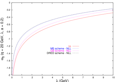
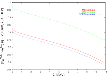
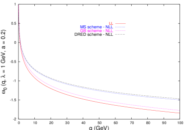
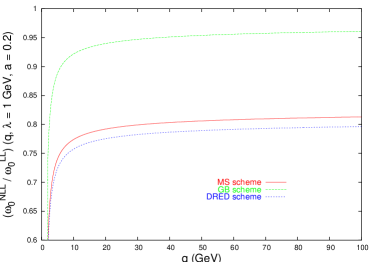
Figure 1: Comparison of the LL and NLL gluon Regge trajectory calculated in different schemes.

Secondly, the part of the real emission kernel in Eq. (8), can be written as

$$\widetilde{\mathcal{K}}_{r}\left(q,q^{\prime},\theta\right)~{}=~{}\frac{a^{2}}{4\pi}\left\{-\frac{1}{\left(q^{2}+{q^{\prime}}^{2}-2\,q\,q^{\prime}\,\cos{\theta}\right)}\ln^{2}{\frac{q^{2}}{{q^{\prime}}^{2}}}\right.$$

$$+\frac{2(q^{2}-{q^{\prime}}^{2})}{\left((q^{2}+{q^{\prime}}^{2})^{2}-4\,q^{2}\,{q^{\prime}}^{2}\,\cos^{2}{\theta}\right)}\left(\frac{1}{2}\ln{\frac{q^{2}}{{q^{\prime}}^{2}}}\ln{\frac{{q}^{2}{q^{\prime}}^{2}\left({q}^{2}+{q^{\prime}}^{2}-2\,q\,q^{\prime}\,\cos{\theta}\right)^{2}}{({q}^{2}+{q^{\prime}}^{2})^{4}}}\right.$$

$$\hskip 28.45274pt\left.+\left(\int_{0}^{-{q}^{2}/{q^{\prime}}^{2}}-\int_{0}^{-{q^{\prime}}^{2}/{q}^{2}}\right)dt\frac{\ln(1-t)}{t}\right)$$

$$\left.-\frac{2\,q\,{q^{\prime}}\,\left|\sin{\theta}\right|}{\left(q^{2}-{q^{\prime}}^{2}\right)^{2}+4\,q^{2}\,{q^{\prime}}^{2}\,\sin^{2}{\theta}}\left(\mathcal{F}\left(q,q^{\prime},\theta\right)+\mathcal{F}\left(q^{\prime},q,\theta\right)\right)\right\},$$ (28)

with $\theta$ being the angle between the two–dimensional vectors $\vec{q}$ and $\vec{q}^{\prime}$. For the function $\mathcal{F}\left(q,q^{\prime},\theta\right)$ we use the expression

$$\mathcal{F}\left(q,q^{\prime},\theta\right)~{}=~{}{\rm Im}\left\{4\,{\rm Li}_{2}\left(\frac{q}{q^{\prime}}\,e^{-i\left|\theta\right|}\right)-\ln{\frac{q^{2}}{{q^{\prime}}^{2}}}\ln{\frac{q^{\prime}\,\left|\sin{\theta}\right|-i\left(q-q^{\prime}\,\cos{\theta}\right)}{q^{\prime}\,\left|\sin{\theta}\right|+i\left(q-q^{\prime}\,\cos{\theta}\right)}}\right\}$$ (29)

with

$${\rm Li}_{2}\left(z\right) = -\int^{z}_{0}dt\frac{\ln(1-t)}{t}.$$ (30)

As in the QCD case, see Ref.[15], this kernel has integrable singularities at $\vec{q}=\vec{q}^{\prime},\vec{q}=0$ and $\vec{q}^{\prime}=0$. This structure is revealed when the kernel is plotted as in Fig. 2 where $\widetilde{\mathcal{K}}_{r}\left(q,q^{\prime}=20~{}{\rm GeV},\theta\right)$ is shown for $a=0.2$ in the ${\overline{\rm MS}}$ scheme. Note how this kernel is positive in a large region of phase space, contrary to the QCD case [15].

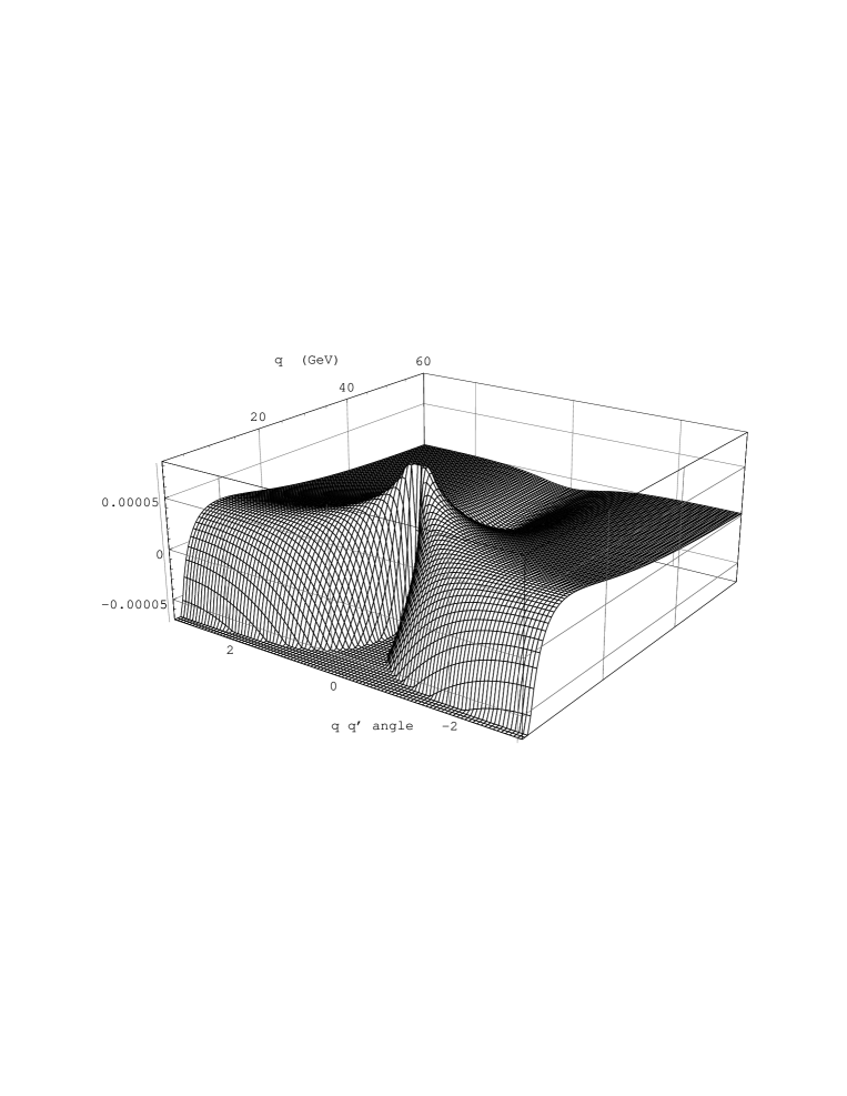
Figure 2: Structure of the kernel $\tilde{K}_{r}\left(q,q^{\prime},\theta\right)$ for $q^{\prime}=20$ GeV as a function of $q$ and the angle between $\vec{q}$ and $\vec{q}^{\prime}$ for the coupling $a=0.2$.

5 Study of the gluon Green’s function

The eigenvalues of the NLL BFKL kernel as in Eq. (10), $\omega_{n}(a,\gamma)$, along the line $\gamma=\frac{1}{2}+i\nu$ for a value of the coupling of $a=0.2$ are plotted in Fig. 3. This line parameterises the contour of the $\gamma$ integration in Eq. (9). The LL eigenvalues are compared to those obtained at NLL for several values of the conformal spin. At high energies, for $n>0$ the relevant region is the one close to $\nu=0$. The zero conformal spin evolution is governed by the two maxima and is the dominant contribution among all conformal spins. We will come back to this figure when the evolution with energy of the different contributions to the gluon Green’s function is studied below.

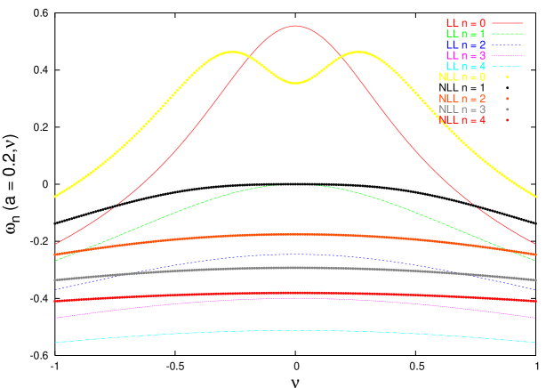
Figure 3: The eigenvalues of the BFKL kernel as a function of $\gamma=\frac{1}{2}+i\nu$ at LL and NLL for different values of the conformal spin $n=0,1,2,3,4$ and a coupling of $a=0.2$.

Very importantly, for a Regge–like choice of energy scale, the NLL kernel in the N = 4 SYM theory does not develop an imaginary part along the $\gamma=\frac{1}{2}+i\nu$ contour. This implies that the asymptotic behaviour at large $Y$ is well controlled and that the gluon Green’s function is monotonically growing with energy. To illustrate this point, we plot in Fig. 4 the angular averaged gluon Green’s function up to very large $Y$ both at LL and NLL accuracy.

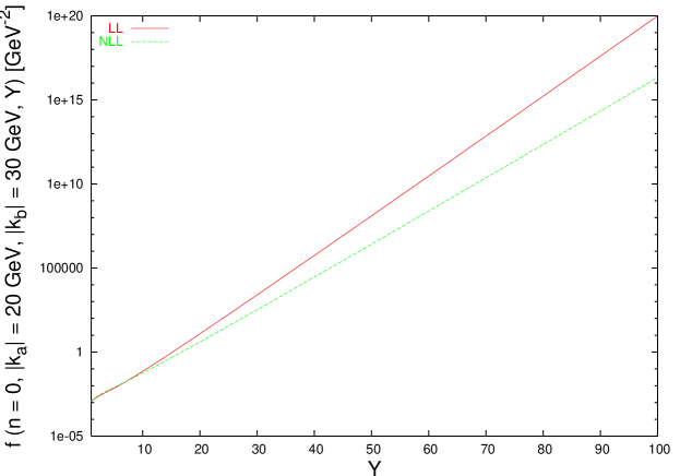
Figure 4: The gluon Green’s function for zero conformal spin for fixed values of the external scales, a coupling of $a=0.2$ and large values of the energy scale Y.

With the intention to confirm the calculation of the conformal spins in N = 4 SYM of Ref. [6] the two methods of solution, that in Mellin space described in Section 2, and the one proposed in this work directly in transverse momentum space as explained in Section 3, will be used to calculate the behaviour of the Green’s function for different conformal spins. To proceed, Eq. (9) can be written as

$$f\left(\vec{k}_{a},\vec{k}_{b},{\rm Y}\right) = \sum_{n=-\infty}^{\infty}f_{n}\left(|\vec{k}_{a}|,|\vec{k}_{b}|,{\rm Y}\right)e^{in\theta},$$ (31)

and the coefficients in the expansion can be calculated following the solution in Mellin space, i.e.

$$f_{n}\left(|\vec{k}_{a}|,|\vec{k}_{b}|,{\rm Y}\right) = \frac{1}{\pi|\vec{k}_{a}||\vec{k}_{b}|}\int\frac{d\gamma}{2\pi i}\left(\frac{\vec{k}_{a}^{2}}{\vec{k}_{b}^{2}}\right)^{\gamma-\frac{1}{2}}e^{\omega_{n}(a,\gamma){\rm Y}},$$ (32)

or they can be obtained using the solution in $\vec{k}$ space, for this it is needed to project on angles, i.e.

$$f_{n}\left(|\vec{k}_{a}|,|\vec{k}_{b}|,{\rm Y}\right) = \int_{0}^{2\pi}\frac{d\theta}{2\pi}\,f\left(\vec{k}_{a},\vec{k}_{b},{\rm Y}\right)\cos{\left(n\theta\right)}.$$ (33)

Therefore the projections on conformal spins can be compared to each other using two completely independent approaches. The results obtained from both solutions are shown in Fig. 5. Both methods exactly coincide in their predictions. This confirms the validity of the results calculated in Ref. [6] and it is a very serious test of the method first proposed in Ref. [14, 15] to study the gluon Green’s function at NLL. As expected from Fig. 3, the dominant conformal spin is $n=0$, whose corresponding eigenvalue is the only positive one at $\nu=0$ in Fig. 3. The eigenvalue at $\nu=0$ for the $n=1$ conformal spin is zero, and thus it is expected to give a constant contribution at large energies. This behaviour is indeed observed in Fig. 5. For the rest of conformal spins their contributions to the gluon Green’s function decrease as the available energy is larger, their eigenvalue being negative at the vecinity of $\nu=0$.

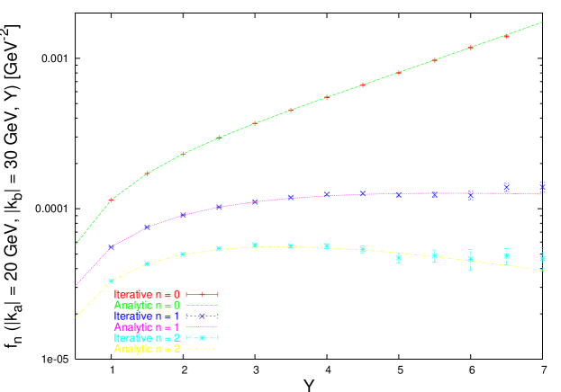
Figure 5: Contributions to the gluon Green’s function from different conformal spins as a function of energy.

A natural question is the convergence in $n$ of the angular expansion of Eq. (31). As the method of solution proposed in this paper allows for a full determination of the angular dependence it is possible to answer this point in a simple manner. This issue is addressed in Fig. 6 where the gluon Green’s function is plotted as function of the angle between the two transverse momenta. Here it can be seen that the conformal expansion reaches good convergence for conformal spins above $n=8$ for the chosen values of $Y$. This plot confirms again that both approaches produce exactly the same results. The graph is produced for two different energies showing a stronger angular correlation for lower energies (the curve is flatter in $\theta$ for $Y=5$), a consequence of the increasing dominance of the zero conformal spin at larger energies.

Figure 6: The dependence of the gluon Green’s function on the angle between the transverse momenta $\vec{k}_{a}$ and $\vec{k}_{b}$.

6 Conclusions

The solution to the NLL BFKL equation for the N = 4 supersymmetric Yang–Mills field theory has been studied in detail. In particular, a newly proposed method of solution has been used which allows for a detailed study of the dependence of the gluon Green’s function on the conformal spins. The results of this work confirm that the calculations of Ref. [6] are correct and, simultaneously, that the proposed method of solution of Ref. [14, 15] for the NLL BFKL equation provides the true answer and accurate description of angular dependences in the multigluon ladder. The growth with energy of the gluon Green’s function for the Regge–like choice of scale has also been demonstrated.

Acknowledgements We thank Tolya Kotikov and Lev Lipatov for very useful discussions, the CERN Theory Division for hospitality, and the IPPP, University of Durham, for use of computer resources. J.R.A. wishes to thank the II. Institut für Theoretische Physik, University of Hamburg, and A.S.V. thanks the Cavendish Laboratory at the University of Cambridge for hospitality.

References

• [1] L. N. Lipatov, Sov. J. Nucl. Phys.  23 (1976) 338 [Yad. Fiz.  23 (1976) 642],
E. A. Kuraev, L. N. Lipatov and V. S. Fadin, Sov. Phys. JETP 45 (1977) 199 [Zh. Eksp. Teor. Fiz.  72 (1977) 377],
I. I. Balitsky and L. N. Lipatov, Sov. J. Nucl. Phys.  28 (1978) 822 [Yad. Fiz.  28 (1978) 1597].
• [2] L.N. Lipatov, JETP ${\bf{63}}$, 904 (1986),
G. Camici and M. Ciafaloni, Phys. Lett. B ${\bf{395}}$, 118 (1997),
R. S. Thorne, Phys. Lett. B 474 (2000) 372, Phys. Rev. D 64 (2001) 074005,
J. R. Forshaw, D. A. Ross and A. Sabio Vera, Phys. Lett. B 498 (2001) 149,
M. Ciafaloni, M. Taiuti and A. H. Mueller, Nucl. Phys. B 616 (2001) 349,
M. Ciafaloni, D. Colferai, G. P. Salam and A. M. Stasto, Phys. Lett. B 541 (2002) 314, Phys. Rev. D 66 (2002) 054014.
• [3] V. S. Fadin and L. N. Lipatov, Phys. Lett. B 429 (1998) 127.
• [4] M. Ciafaloni and G. Camici, Phys. Lett. B 430 (1998) 349.
• [5] D.A. Ross, Phys. Lett. B431 (1998) 161,
Yu.V. Kovchegov and A.H. Mueller, Phys. Lett. B439 (1998) 423,
J. Blümlein, V. Ravindran, W.L. van Neerven and A. Vogt, preprint DESY-98-036, hep-ph/9806368,
E.M. Levin, preprint TAUP 2501-98, hep-ph/9806228,
N. Armesto, J. Bartels, M.A. Braun, Phys. Lett. B442 (1998) 459,
G.P. Salam, JHEP 8907 (1998) 19,
M. Ciafaloni and D. Colferai, Phys. Lett. B452 (1999) 372,
M. Ciafaloni, D. Colferai and G.P. Salam, Phys. Rev. D60 (1999) 114036,
R.S. Thorne, Phys. Rev. D60 (1999) 054031,
S. J. Brodsky, V. S. Fadin, V. T. Kim, L. N. Lipatov and G. B. Pivovarov, JETP Lett.  70 (1999) 155,
C. R. Schmidt, Phys. Rev. D 60 (1999) 074003,
J. R. Forshaw, D. A. Ross and A. Sabio Vera, Phys. Lett. B 455 (1999) 273,
G. Altarelli, R. D. Ball and S. Forte, Nucl. Phys. B 575 (2000) 313, Nucl. Phys. B 621 (2002) 359, Nucl. Phys. B 674 (2003) 459,
M. Ciafaloni, D. Colferai, G. P. Salam and A. M. Stasto, Phys. Lett. B 576 (2003) 143, Phys. Rev. D 68 (2003) 114003, Phys. Lett. B 587 (2004) 87.
• [6] A. V. Kotikov and L. N. Lipatov, Nucl. Phys. B 582 (2000) 19, Nucl. Phys. B 661 (2003) 19 [Erratum-ibid. B 685 (2004) 405].
• [7] A. V. Kotikov, L. N. Lipatov and V. N. Velizhanin, Phys. Lett. B 557 (2003) 114.
• [8] A. V. Kotikov, L. N. Lipatov, A. I. Onishchenko and V. N. Velizhanin, hep-th/0404092.
• [9] S. Moch, J. A. M. Vermaseren and A. Vogt, Nucl. Phys. B 688 (2004) 101.
• [10] A. Vogt, S. Moch and J. A. M. Vermaseren, hep-ph/0404111.
• [11] J. Kwiecinski, C. A. M. Lewis and A. D. Martin, Phys. Rev. D 54 (1996) 6664
• [12] C. R. Schmidt, Phys. Rev. Lett.  78 (1997) 4531
• [13] L. H. Orr and W. J. Stirling, Phys. Rev. D 56 (1997) 5875
• [14] J. R. Andersen and A. Sabio Vera, Phys. Lett. B 567 (2003) 116.
• [15] J. R. Andersen and A. Sabio Vera, Nucl. Phys. B 679 (2004) 345.