Chern-Simons Theory and Topological Strings

Abstract

We review the relation between Chern-Simons gauge theory and topological string theory on noncompact Calabi-Yau spaces. This relation has made possible to give an exact solution of topological string theory on these spaces to all orders in the string coupling constant. We focus on the construction of this solution, which is encoded in the topological vertex, and we emphasize the implications of the physics of string/gauge theory duality for knot theory and for the geometry of Calabi-Yau manifolds.

I Introduction

Even though string theory has not found yet a clear place in our understanding of Nature, it has already established itself as a source of fascinating results and research directions in mathematics. In recent years, string theory and some of its close cousins (like conformal field theory and topological field theory) have had an enormous impact in representation theory, differential geometry, low-dimensional topology, and algebraic geometry.

One mathematical area which has been deeply influenced by conformal field theory and topological field theory is knot theory. Witten (1989) found that many topological invariants of knots and links discovered in the 1980s (like the Jones and the HOMFLY polynomials) could be reinterpreted as correlation functions of Wilson loop operators in Chern-Simons theory, a gauge theory in three dimensions with topological invariance. Witten also showed that the partition function of this theory provided a new topological invariant of three-manifolds, and by working out the exact solution of Chern-Simons gauge theory he made a connection between these knot and three-manifold invariants and conformal field theory in two dimensions (in particular, the Wess-Zumino-Witten model).

In a seemingly unrelated development, it was found that the study of string theory on Calabi-Yau manifolds (which was triggered by the phenomenological interest of the resulting four-dimensional models) provided new insights in the geometry of these spaces. Some correlation functions of string theory on Calabi-Yau manifolds turn out to compute numbers of holomorphic maps from the string worldsheet to the target, therefore they contain information about the enumerative geometry of the Calabi-Yau spaces. This led to the introduction of Gromov-Witten invariants in mathematics as a way to capture this information. Moreover, the existence of a powerful duality symmetry of string theory in Calabi-Yau spaces -mirror symmetry- allowed the computation of generating functions for these invariants, and made possible to solve with physical techniques difficult enumerative problems (see Hori et al., 2003, for a review of these developments). The existence of a topological sector in string theory which captured the enumerative geometry of the target space led also to the construction of simplified models of string theory which kept only the topological information of the more complicated, physical theory. These models are called topological string theories and turn out to provide in many cases exactly solvable models of string dynamics.

The key idea that allowed to build a bridge between topological string theory and Chern-Simons theory was the gauge theory/string theory correspondence. It is an old idea, going back to ‘t Hooft (1974) that gauge theories can be described in the $1/N$ expansion by string theories. This idea has been difficult to implement, but in recent years some spectacular progress was made thanks to the work of Maldacena (1998), who found a duality between type IIB string theory on ${\rm AdS}_{5}\times{\bf S}^{5}$ and ${\cal N}=4$ super Yang-Mills with gauge group $U(N)$. It is then natural to ask if gauge theories which are simpler than ${\cal N}=4$ Yang-Mills -like for example Chern-Simons theory- also admit a string theory description. It was shown by Gopakumar and Vafa (1999) that Chern-Simons gauge theory on the three-sphere has in fact a closed string description in terms of topological string theory propagating on a particular Calabi-Yau target, the so-called resolved conifold.

The result of Gopakumar and Vafa has three important consequences. First of all, it provides a toy model of the gauge theory/string theory correspondence which makes possible to test in detail general ideas about this duality. Second, it gives a stringy interpretation of invariants of knots in the three-sphere. More precisely, it establishes a relation between invariants of knots based on quantum groups, and Gromov-Witten invariants of open strings propagating on the resolved conifold. These are a priori two very different mathematical objects, and in this way the physical idea of a correspondence between gauge theories and strings gives new and fascinating results in mathematics that we are only starting to unveil. Finally, one can use the results of Gopakumar and Vafa to completely solve topological string theory on certain Calabi-Yau threefolds in a closed form. As we will see, this gives the all-genus answer for certain string amplitudes, and it is in fact one of the few examples in string theory where such an answer is available. The all-genus solution to the amplitudes also encodes the information about all the Gromov-Witten invariants for those threefolds. Since the solution involves building blocks from Chern-Simons theory, it suggests yet another bridge between knot invariants and Gromov-Witten theory.

In this review we will focus on this last aspect. The organization of the review is the following: in section II we give an introduction to the relevant aspects of Chern-Simons theory that will be needed for the applications to Calabi-Yau geometry. In particular, we give detailed results for the computation of the relevant knots and link invariants. In section III we give a short review on the $1/N$ expansion of Chern-Simons theory, which is the approach that makes possible the connection to string theory. Section IV contains a review of closed and open topological string theory on Calabi-Yau threefolds, and we construct in full detail the geometry of non-compact, toric Calabi-Yau spaces, since these are the manifolds that we will be able to study by using the gauge theory/string theory correspondence. In section V we establish the correspondence between Chern-Simons theory on the three-sphere and closed topological string theory on a resolved conifold. In section VI we show how the arguments of section V can be extended to construct gauge theory duals of topological string theory on more complicated non-compact, toric Calabi-Yau manifolds. In section VII we complete this program by defining the topological vertex, an object that allows to solve topological string theory on all non-compact, toric Calabi-Yau threefolds by purely combinatorial methods. We also give a detailed derivation of the topological vertex from Chern-Simons theory, and we give various applications of the formalism. The last section contains some conclusions and open directions for further research. A short Appendix contains some elementary facts about the theory of symmetric polynomials that are used in the review.

There are many issues that we have not analyzed in detail in this review. For example, we have not discussed the mirror-symmetric side of the story, and we do not address in detail the relation between topological string amplitudes and type II superstring amplitudes. We refer the reader to the excellent book by Hori et al. (2003) for an introduction to these topics. Other reviews of the topics discussed here can be found in Grassi and Rossi (2002) and Mariño (2002b).

II Chern-Simons theory and knot invariants

II.1 Chern-Simons theory: basic ingredients

In a groundbreaking paper, Witten (1989) showed that Chern-Simons gauge theory, which is a quantum field theory in three dimensions, provides a physical description of a wide class of invariants of three-manifolds and of knots and links in three-manifolds. The Chern-Simons action with gauge group $G$ on a generic three-manifold $M$ is defined by

$$S={k\over 4\pi}\int_{M}{\rm Tr}\Bigl{(}A\wedge dA+{2\over 3}A\wedge A\wedge A\Bigr{)}$$ (1)

Here, $k$ is the coupling constant, and $A$ is a $G$-gauge connection on the trivial bundle over $M$. In this review we will mostly consider Chern-Simons theory with gauge group $G=U(N)$. As noticed by Witten (1989), since this action does not involve the metric, the resulting quantum theory is topological, at least formally. In particular, the partition function

$$Z(M)=\int[{\cal D}A]{\rm e}^{iS}$$ (2)

should define a topological invariant of the manifold $M$. A detailed analysis shows that this is in fact the case, with an extra subtlety: the invariant depends not only on the three-manifold but also on a choice of framing (i.e. a choice of trivialization of the bundle $TM\oplus TM$). As explained by Atiyah (1990), for every three-manifold there is a canonical choice of framing, and the different choices are labelled by an integer $s\in{\bf Z}$ in such a way that $s=0$ corresponds to the canonical framing. In the following all the results for the partition functions will be presented in the canonical framing.

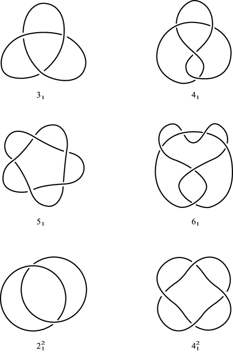
Figure 1: Some knots and links. In the notation $x_{n}^{L}$, $x$ indicates the number of crossings, $L$ the number of components (in case it is a link with $L>1$) and $n$ is a number used to enumerate knots and links in a given set characterized by $x$ and $L$. The knot $3_{1}$ is also known as the trefoil knot, while $4_{1}$ is known as the figure-eight knot. The link $2_{1}^{2}$ is called the Hopf link.

Besides providing invariants of three-manifolds, Chern-Simons theory also provides invariants of knots and links inside three-manifolds (for a survey of modern knot theory, see Lickorish (1998) and Prasolov and Sossinsky (1997)). Some examples of knots and links are depicted in Fig. 1. Given an oriented knot ${\cal K}$ in ${\bf S}^{3}$, we can consider the trace of the holonomy of the gauge connection around $\cal K$ in a given irreducible representation $R$ of $U(N)$, which gives the Wilson loop operator:

$$W^{\cal K}_{R}(A)={\rm Tr}_{R}U_{\cal K}$$ (3)

where

$$U_{\cal K}={\rm P}\,\exp\,\oint_{\cal K}A$$ (4)

is the holonomy around the knot. (3) is a gauge invariant operator whose definition does not involve the metric on the three-manifold. The irreducible representations of $U(N)$ will be labelled by highest weights or equivalently by the lengths of rows in a Young tableau, $l_{i}$, where $l_{1}\geq l_{2}\geq\cdots$. If we now consider a link ${\cal L}$ with components ${\cal K}_{\alpha}$, $\alpha=1,\cdots,L$, we can in principle compute the correlation function,

$$\displaystyle W_{R_{1}\cdots R_{L}}({\cal L}) = \langle W^{{\cal K}_{1}}_{R_{1}}\cdots W^{{\cal K}_{L}}_{R_{L}}\rangle$$ (5)

$$= {1\over Z(M)}\int[{\cal D}A]\Bigl{(}\prod_{\alpha=1}^{L}W_{R_{\alpha}}^{{\cal K}_{\alpha}}\Bigr{)}{\rm e}^{iS}.$$

The topological character of the action, and the fact that the Wilson loop operators can be defined without using any metric on the three-manifold, indicate that (5) is a topological invariant of the link ${\cal L}$. Notice that we are taking the knots and links to be oriented, and this makes a difference. If ${\cal K}^{-1}$ denotes the knot obtained from ${\cal K}$ by inverting its orientation, we have that

$${\rm Tr}_{R}U_{{\cal K}^{-1}}={\rm Tr}_{R}U^{-1}_{\cal K}={\rm Tr}_{\overline{R}}U_{\cal K},$$ (6)

where ${\overline{R}}$ denotes the conjugate representation. For further use we notice that, given two linked oriented knots ${\cal K}_{1}$, ${\cal K}_{2}$, one can define a elementary topological invariant, the linking number, by

$${\rm lk}({\cal K}_{1},{\cal K}_{2})={1\over 2}\sum_{\rm p}\epsilon(p),$$ (7)

where the sum is over all crossing points, and $\epsilon(p)=\pm 1$ is a sign associated to the crossings as indicated in Fig.  2. The linking number of a link ${\cal L}$ with components ${\cal K}_{\alpha}$, $\alpha=1,\cdots,L$, is defined by

$${\rm lk}({\cal L})=\sum_{\alpha<\beta}{\rm lk}({\cal K}_{\alpha},{\cal K}_{\beta}).$$ (8)

Figure 2: When computing the linking number of two knots, the crossings are assigned a sign $\pm 1$ as indicated in the figure.

Some of the correlation functions of Wilson loops in Chern-Simons theory turn out to be closely related to important polynomial invariants of knots and links. For example, one of the most important polynomial invariants of a link ${\cal L}$ is the HOMFLY polynomial $P_{\cal L}(q,\lambda)$, which depends on two variables $q$ and $\lambda$ and was introduced by Freyd et al. (1985). This polynomial turns out to be related to the correlation function (5) when the gauge group is $U(N)$ and all the components are in the fundamental representation $R_{\alpha}=\vbox{\offinterlineskip\kern 1.0pt\hbox{\kern 1.0pt\vbox{\hbox{\noindent\vbox{\hbox{\vbox to0.0pt{\hrule height=0.4pt,width=3.90555pt\vss}}\hbox{\vbox{\hbox to0.0pt{\vrule width=0.4pt,height=3.90555pt\hss}}\kern 3.90555pt\vbox{\hbox to0.0pt{\vrule width=0.4pt,height=3.90555pt\hss}}}\hbox{\vbox{\hbox{\vbox to0.0pt{\hrule height=0.4pt,width=4.30554pt\vss}}}\kern-0.4pt}}}\hbox{} }\kern 1.0pt\kern 0.4pt}\kern 1.0pt\kern 0.4pt}$. More precisely, we have

$$W_{\vbox{\offinterlineskip\kern 1.0pt\hbox{\kern 1.0pt\vbox{\hbox{\noindent\vbox{\hbox{\vbox to0.0pt{\hrule height=0.4pt,width=3.90555pt\vss}}\hbox{\vbox{\hbox to0.0pt{\vrule width=0.4pt,height=3.90555pt\hss}}\kern 3.90555pt\vbox{\hbox to0.0pt{\vrule width=0.4pt,height=3.90555pt\hss}}}\hbox{\vbox{\hbox{\vbox to0.0pt{\hrule height=0.4pt,width=4.30554pt\vss}}}\kern-0.4pt}}}\hbox{} }\kern 1.0pt\kern 0.4pt}\kern 1.0pt\kern 0.4pt}\cdots\vbox{\offinterlineskip\kern 1.0pt\hbox{\kern 1.0pt\vbox{\hbox{\noindent\vbox{\hbox{\vbox to0.0pt{\hrule height=0.4pt,width=3.90555pt\vss}}\hbox{\vbox{\hbox to0.0pt{\vrule width=0.4pt,height=3.90555pt\hss}}\kern 3.90555pt\vbox{\hbox to0.0pt{\vrule width=0.4pt,height=3.90555pt\hss}}}\hbox{\vbox{\hbox{\vbox to0.0pt{\hrule height=0.4pt,width=4.30554pt\vss}}}\kern-0.4pt}}}\hbox{} }\kern 1.0pt\kern 0.4pt}\kern 1.0pt\kern 0.4pt}}({\cal L})=\lambda^{{\rm lk}({\cal L})}\biggl{(}{\lambda^{1\over 2}-\lambda^{-{1\over 2}}\over q^{1\over 2}-q^{-{1\over 2}}}\biggr{)}P_{\cal L}(q,\lambda)$$ (9)

where ${\rm lk}({\cal L})$ is the linking number of ${\cal L}$, and the variables $q$ and $\lambda$ are related to the Chern-Simons variables as

$$q=\exp\biggl{(}{2\pi i\over k+N}\biggr{)},\quad\lambda=q^{N}.$$ (10)

When $N=2$ the HOMFLY polynomial reduces to a one-variable polynomial, the Jones polynomial. When the gauge group of Chern-Simons theory is $SO(N)$, $W_{\vbox{\offinterlineskip\kern 1.0pt\hbox{\kern 1.0pt\vbox{\hbox{\noindent\vbox{\hbox{\vbox to0.0pt{\hrule height=0.4pt,width=3.90555pt\vss}}\hbox{\vbox{\hbox to0.0pt{\vrule width=0.4pt,height=3.90555pt\hss}}\kern 3.90555pt\vbox{\hbox to0.0pt{\vrule width=0.4pt,height=3.90555pt\hss}}}\hbox{\vbox{\hbox{\vbox to0.0pt{\hrule height=0.4pt,width=4.30554pt\vss}}}\kern-0.4pt}}}\hbox{} }\kern 1.0pt\kern 0.4pt}\kern 1.0pt\kern 0.4pt}\cdots\vbox{\offinterlineskip\kern 1.0pt\hbox{\kern 1.0pt\vbox{\hbox{\noindent\vbox{\hbox{\vbox to0.0pt{\hrule height=0.4pt,width=3.90555pt\vss}}\hbox{\vbox{\hbox to0.0pt{\vrule width=0.4pt,height=3.90555pt\hss}}\kern 3.90555pt\vbox{\hbox to0.0pt{\vrule width=0.4pt,height=3.90555pt\hss}}}\hbox{\vbox{\hbox{\vbox to0.0pt{\hrule height=0.4pt,width=4.30554pt\vss}}}\kern-0.4pt}}}\hbox{} }\kern 1.0pt\kern 0.4pt}\kern 1.0pt\kern 0.4pt}}({\cal L})$ is closely related to the Kaufmann polynomial. For the mathematical definition and properties of these polynomials, see for example Lickorish (1998).

II.2 Perturbative approach

The partition function and correlation functions of Wilson loops in Chern-Simons theory can be computed in a variety of ways. One can for example use standard perturbation theory. In the computation of the partition function in perturbation theory, we have to find first the classical solutions of the Chern-Simons equations of motion. If we write $A=\sum_{a}A^{a}T_{a}$, where $T_{a}$ is a basis of the Lie algebra, we find

$${\delta S\over\delta A^{a}_{\mu}}={k\over 4\pi}\epsilon^{\mu\nu\rho}F^{a}_{\nu\rho},$$

therefore the classical solutions are just flat connections on $M$. Flat connections are in one-to-one correspondence with group homomorphisms

$$\pi_{1}(M)\rightarrow G.$$ (11)

For example, if $M={\bf S}^{3}/{\bf Z}_{p}$ is the lens space $L(p,1)$, one has $\pi_{1}(L(p,1))={\bf Z}_{p}$, and flat connections are labeled by homomorphisms ${\bf Z}_{p}\rightarrow G$. Let us assume that these are a discrete set of points (this happens, for example, if $M$ is a rational homology sphere, since in that case $\pi_{1}(M)$ is a finite group). In that situation, one expresses $Z(M)$ as a sum of terms associated to stationary points:

$$Z(M)=\sum_{c}Z^{(c)}(M),$$ (12)

where $c$ labels the different flat connections $A^{(c)}$ on $M$. Each of the $Z^{(c)}(M)$ will be an asympotic series in $1/k$ of the form

$$Z^{(c)}(M)=Z^{(c)}_{\rm 1-loop}(M).\exp\Biggl{\{}\sum_{\ell=1}^{\infty}S^{(c)}_{\ell}x^{\ell}\Biggr{\}}.$$ (13)

In this equation, $x$ is the effective expansion parameter:

$$x={2\pi i\over k+y},$$ (14)

and $y$ is the dual Coxeter number of the group (for $G=U(N)$, $y=N$). The one-loop correction $Z^{(c)}_{\rm 1-loop}(M)$ was first analyzed by Witten (1989), and has been studied in great detail since then (Freed and Gompf, 1991; Jeffrey, 1992; Rozansky, 1995). It has the form

$$Z^{(c)}_{\rm 1-loop}(M)\propto{{\sqrt{|\tau^{(c)}_{R}|}\over{\rm vol}(H_{c})}},$$ (15)

where $\tau^{(c)}_{R}$ is the Reidemeister-Ray-Singer torsion of $A^{(c)}$ and $H_{c}$ is the isotropy group of $A^{(c)}$. Notice that, for the trivial flat connection $A^{(c)}=0$, $H_{c}=G$.

The terms $S^{(c)}_{\ell}$ in (13) correspond to connected diagrams with $2\ell$ vertices. In Chern-Simons theory the vertex is trivalent, so $S^{(c)}_{\ell}$ is the contribution to the free energy at $\ell+1$ loops. The contributions of the trivial connection will be denoted simply by $S_{\ell}$. Notice that the computation of $S^{(c)}_{\ell}$ involves the evaluation of group factors of Feynman diagrams, and therefore they depend explicitly on the gauge group $G$. When $G=U(N)$, they are polynomials in $N$. For example, $S_{1}$ contains the group factor $2N(N^{2}-1)$.

The perturbative evaluation of Wilson loop correlators can also be done using standard procedures. First of all one has to expand the holonomy operator as

$$W_{R}^{\cal K}(A)={\rm Tr}_{R}\biggl{[}{\bf 1}+\oint_{\cal K}dx^{\mu}A_{\mu}(x)$$ (16)

$$+ \oint_{\cal K}dx^{\mu}\int^{x}dy^{\nu}A_{\nu}(y)A_{\mu}(x)+\cdots\biggr{]},$$

where $A_{\mu}=\sum_{a}A_{\mu}^{a}T_{a}$. Then, after gauge fixing, one can proceed and evaluate the correlation functions in standard perturbation theory. The perturbative study of Wilson loops was started by Guadagnini, Martellini, and Mintchev (1990). A nice review of its development can be found in Labastida (1999). Here we will rather focus on the nonperturbative approach to Chern-Simons theory, which we now explain.

II.3 Canonical quantization and surgery

As it was shown by Witten (1989), Chern-Simons theory is exactly solvable by using nonperturbative methods and the relation to the Wess-Zumino-Witten (WZW) model. In order to present this solution, it is convenient to recall some basic facts about the canonical quantization of the model.

Let $M$ be a three-manifold with boundary given by a Riemann surface $\Sigma$. We can insert a general operator ${\cal O}$ in $M$, which will be in general a product of Wilson loops along different knots and in arbitrary representations of the gauge group. We will consider the case in which the Wilson loops do not intersect the surface $\Sigma$. The path integral over the three-manifold with boundary $M$ gives a wavefunction $\Psi_{M,\cal O}({\cal A})$ which is a functional of the values of the field at $\Sigma$. Schematically we have:

$$\Psi_{M,\cal O}({\cal A})=\langle{\cal A}|\Psi_{M,\cal O}\rangle=\int_{A|_{\Sigma}={\cal A}}{\cal D}A\,{\rm e}^{iS}\,{\cal O}.$$ (17)

In fact, associated to the Riemann surface $\Sigma$ we have a Hilbert space ${\cal H}(\Sigma)$, which can be obtained by doing canonical quantization of Chern-Simons theory on $\Sigma\times{\bf R}$. Before spelling out in detail the structure of these Hilbert spaces, let us make some general considerations about the computation of physical quantities.

In the context of canonical quantization, the partition function can be computed as follows. We first perform a Heegaard splitting of the three-manifold, i.e. we represent it as the connected sum of two three-manifolds $M_{1}$ and $M_{2}$ sharing a common boundary $\Sigma$, where $\Sigma$ is a Riemann surface. If $f:\Sigma\rightarrow\Sigma$ is an homeomorphism, we will write $M=M_{i}\cup_{f}M_{2}$, so that $M$ is obtained by gluing $M_{1}$ to $M_{2}$ through their common boundary and using the homeomorphism $f$. This is represented in Fig. 3. We can then compute the full path integral (2) over $M$ by computing first the path integral over $M_{1}$ to obtain a state $|\Psi_{M_{1}}\rangle$ in ${\cal H}(\Sigma)$. The boundary of $M_{2}$ is also $\Sigma$, but with opposite orientation, so its Hilbert space is the dual space ${\cal H}^{*}(\Sigma)$. The path integral over $M_{2}$ produces then a state $\langle\Psi_{M_{2}}|\in{\cal H}^{*}(\Sigma)$. The homeomorphism $f:\Sigma\rightarrow\Sigma$ will be represented by an operator acting on ${\cal H}(\Sigma)$,

$$U_{f}:{\cal H}(\Sigma)\rightarrow{\cal H}(\Sigma).$$ (18)

and the partition function can be finally evaluated as

$$Z(M)=\langle\Psi_{M_{2}}|U_{f}|\Psi_{M_{1}}\rangle.$$ (19)

Therefore, if we know explicitly what the wavefunctions and the operators associated to homeomorphisms are, we can compute the partition function.

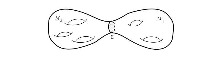
Figure 3: Heegaard splitting of a three-manifold $M$ into two three manifolds $M_{1}$ and $M_{2}$ with a common boundary $\Sigma$.

One of the most fundamental results of Witten (1989) is in fact a precise description of ${\cal H}(\Sigma)$: it is the space of conformal blocks of a WZW model on $\Sigma$ with gauge group $G$ and level $k$ (for an extensive review of the WZW model, see for example Di Francesco et al., 1997). In particular, ${\cal H}(\Sigma)$ has finite dimension. We will not review here the derivation of this fundamental result. Instead we will use the relevant information from the WZW model in order to solve Chern-Simons theory.

The description of the space of conformal blocks on Riemann surfaces can be made very explicit when $\Sigma$ is a sphere or a torus. For $\Sigma={\bf S}^{2}$, the space of conformal blocks is one-dimensional, so ${\cal H}({\bf S}^{2})$ is spanned by a single element. For $\Sigma={\bf T}^{2}$, the space of conformal blocks is in one to one correspondence with the integrable representations of the affine Lie algebra associated to $G$ at level $k$. We will use the following notations: the fundamental weights of $G$ will be denoted by $\lambda_{i}$, and the simple roots by $\alpha_{i}$, with $i=1,\cdots,r$, and $r$ denotes the rank of $G$. The weight and root lattices of $G$ are denoted by $\Lambda^{w}$ and $\Lambda^{r}$, respectively, and $|\Delta_{+}|$ denotes the number of positive roots. The fundamental chamber ${\cal F}_{l}$ is given by $\Lambda^{w}/l\Lambda^{r}$, modded out by the action of the Weyl group. For example, in $SU(N)$ a weight $p=\sum_{i=1}^{r}p_{i}\lambda_{i}$ is in ${\cal F}_{l}$ if

$$\sum_{i=1}^{r}p_{i}<l,\,\,\,\,\,\,{\rm and}\,\,\ p_{i}>0,\,i=1,\cdots,r.$$ (20)

We recall that a representation given by a highest weight $\Lambda$ is integrable if $\rho+\Lambda$ is in the fundamental chamber ${\cal F}_{l}$, where $l=k+y$ ($\rho$ denotes as usual the Weyl vector, given by the sum of the fundamental weights). In the following, the states in the Hilbert state of the torus ${\cal H}({\bf T}^{2})$ will be denoted by $|p\rangle=|\rho+\Lambda\rangle$ where $\rho+\Lambda$, as we have stated, is an integrable representation of the WZW model at level $k$. We will also denote these states by $|R\rangle$, where $R$ is the representation associated to $\Lambda$. The state $|\rho\rangle$ will be denoted by $|0\rangle$. The states $|R\rangle$ can be chosen to be orthonormal (Witten, 1989; Elitzur et. al., 1989; Labastida and Ramallo, 1989), so we have

$$\langle R|R^{\prime}\rangle=\delta_{RR^{\prime}}.$$ (21)

There is a special class of homeomorphisms of ${\bf T}^{2}$ that have a simple expression as operators in ${\cal H}({\bf T}^{2})$; these are the ${\rm Sl}(2,{\bf Z})$ transformations. Recall that the group ${\rm Sl}(2,{\bf Z})$ consists of $2\times 2$ matrices with integer entries and unit determinant. If $(1,0)$ and $(0,1)$ denote the two one-cycles of ${\bf T}^{2}$, we can specify the action of an ${\rm Sl}(2,{\bf Z})$ transformation on the torus by giving its action on this homology basis. The ${\rm Sl}(2,{\bf Z})$ group is generated by the transformations $T$ and $S$, which are given by

$$T=\left(\begin{array}[]{cc}1&1\\ 0&1\end{array}\right),\,\,\,\,\,\,\,S=\left(\begin{array}[]{cc}0&-1\\ 1&0\end{array}\right).$$ (22)

Notice that the $S$ transformation exchanges the one-cycles of the torus. These transformations can be lifted to ${\cal H}({\bf T}^{2})$, and they have the following matrix elements in the basis of integrable representations:

$$\displaystyle T_{pp^{\prime}} = \delta_{p,p^{\prime}}{\rm e}^{2\pi i(h_{p}-c/24)},$$

$$S_{pp^{\prime}} = {i^{|\Delta_{+}|}\over(k+y)^{r/2}}\Biggl{(}{{\rm Vol}\,\Lambda^{w}\over{\rm Vol}\,\Lambda^{r}}\Biggr{)}^{1\over 2}$$ (23)

$$\,\,\,\times\sum_{w\in{\cal W}}\epsilon(w)\exp\Bigl{(}-{2\pi i\over k+y}p\cdot w(p^{\prime})\Bigr{)}.$$

In the first equation, $c$ is the central charge of the WZW model, and $h_{p}$ is the conformal weight of the primary field associated to $p$:

$$h_{p}={p^{2}-\rho^{2}\over 2(k+y)},$$ (24)

where we remind that $p$ is of the form $\rho+\Lambda$. In the second equation, the sum over $w$ is a sum over the elements of the Weyl group ${\cal W}$, $\epsilon(w)$ is the signature of the element $w$, and ${\rm Vol}\,\Lambda^{w(r)}$ denote respectively the volume of the weight (root) lattice. We will often write $S_{RR^{\prime}}$ for $S_{pp^{\prime}}$, where $p=\rho+\Lambda$, $p^{\prime}=\rho+\Lambda^{\prime}$ and $\Lambda$, $\Lambda^{\prime}$ are the highest weights corresponding to the representations $R$, $R^{\prime}$.

Figure 4: Performing the path integral on a solid torus with a Wilson line in representation $R$ gives the state $|R\rangle$ in ${\cal H}({\bf T}^{2})$.

What is the description of the states $|R\rangle$ in ${\cal H}({\bf T}^{2})$ from the point of view of canonical quantization? Consider the solid torus ${\cal T}=D\times{\bf S}^{1}$, where $D$ is a disc in ${\bf R}^{2}$. This is a three-manifold whose boundary is a ${\bf T}^{2}$, and it has a noncontractible cycle given by the ${\bf S}^{1}$. Let us now consider the Chern-Simons path integral on the solid torus, with the insertion of the operator ${\cal O}_{R}={\rm Tr}_{R}U$ given by a Wilson loop in the representation $R$ around the noncontractible cycle, as shown in Fig. 4. In this way one obtains a state in ${\cal H}({\bf T}^{2})$, and one has

$$|\Psi_{{\cal T},{\cal O}_{R}}\rangle=|R\rangle.$$ (25)

In particular, the path integral over the solid torus with no operator insertion gives $|0\rangle$, the “vacuum” state.

These results allow us to compute the partition function of any three-manifold that admits a Heegaard splitting along a torus. Imagine for example that we take two solid tori and we glue them along their boundary with the identity map. Since a solid torus is a disc times a circle $D\times{\bf S}^{1}$, by performing this operation we get a manifold which is ${\bf S}^{1}$ times the two discs glued together along their boundaries. Therefore, with this surgery we obtain ${\bf S}^{2}\times{\bf S}^{1}$, and (19) gives then

$$Z({\bf S}^{2}\times{\bf S}^{1})=\langle 0|0\rangle=1.$$ (26)

If we do the gluing, however, after performing an $S$-transformation on the ${\bf T}^{2}$ the resulting manifold is instead ${\bf S}^{3}$. To see this, notice that the complement to a solid torus inside ${\bf S}^{3}$ is indeed another solid torus whose noncontractible cycle is homologous to the contractible cycle in the first torus. We then find

$$Z({\bf S}^{3})=\langle 0|S|0\rangle=S_{00}.$$ (27)

By using Weyl’s denominator formula,

$$\sum_{w\in{\cal W}}\epsilon(w){\rm e}^{w(\rho)}=\prod_{\alpha>0}2\sinh{\alpha\over 2},$$ (28)

where $\alpha>0$ are positive roots, one finds

$$Z({\bf S}^{3})={1\over(k+y)^{r/2}}\Biggl{(}{{\rm Vol}\,\Lambda^{w}\over{\rm Vol}\,\Lambda^{r}}\Biggr{)}^{1\over 2}\prod_{\alpha>0}2\sin\Bigl{(}{\pi(\alpha\cdot\rho)\over k+y}\Bigr{)}.$$ (29)

The above result can be generalized in order to compute path integrals in ${\bf S}^{3}$ with some knots and links. Consider a solid torus where a Wilson line in representation $R$ has been inserted. The corresponding state is $|R\rangle$, as we explained before. If we now glue this to an empty solid torus after an $S$-transformation, we obtain a trivial knot, or unknot, in ${\bf S}^{3}$. The path integral with the insertion is then,

$$Z({\bf S}_{3},{\cal O}_{R})=\langle 0|S|R\rangle.$$ (30)

It follows that the normalized vacuum expectation value for the unknot in ${\bf S}^{3}$, in representation $R$, is given by

$$W_{R}({\rm unknot})={S_{0R}\over S_{00}}={\sum_{w\in{\cal W}}\epsilon(w){\rm e}^{-{2\pi i\over k+y}\rho\cdot w(\Lambda+\rho)}\over\sum_{w\in{\cal W}}\epsilon(w){\rm e}^{-{2\pi i\over k+y}\rho\cdot w(\rho)}}.$$ (31)

Remember that the character of the representation $R$, evaluated on an element $a\in\Lambda_{\rm w}\otimes{\bf R}$ is defined by

$${\rm ch}_{R}(a)=\sum_{\mu\in M_{R}}e^{a\cdot\mu}$$ (32)

where $M_{R}$ is the set of weights associated to the irreducible representation $R$. By using Weyl’s character formula we can write

$$W_{R}({\rm unknot})={\rm ch}_{R}\Bigl{[}-{2\pi i\over k+y}\rho\Bigr{]}.$$ (33)

Moreover, using (28), we finally obtain

$$W_{R}({\rm unknot})=\prod_{\alpha>0}{\sin\Bigl{(}{\pi\over k+y}\alpha\cdot(\Lambda+\rho)\Bigr{)}\over\sin\Bigl{(}{\pi\over k+y}\alpha\cdot\rho\Bigr{)}}$$ (34)

This quantity is often called the quantum dimension of $R$, and it is denoted by ${\rm dim}_{q}R$.

We can also consider a solid torus with Wilson loop in representation $R$, glued to another solid torus with the representation $R^{\prime}$ through an $S$-transformation. What we obtain is clearly a link in ${\bf S}^{3}$ with two components, which is the Hopf link shown in Fig. 1. Taking into account the orientation carefully, we find that this is the Hopf link with linking number $+1$. The path integral with this insertion is:

$$Z({\bf S}^{3},{\cal O}_{R}{\cal O}_{R^{\prime}})=\langle R^{\prime}|S|R\rangle,$$ (35)

so the normalized vacuum expectation value is

$${\cal W}_{RR^{\prime}}\equiv W_{RR^{\prime}}({\rm Hopf}^{+1})={S_{{\overline{R}}^{\prime}R}\over S_{00}}={S^{-1}_{R^{\prime}R}\over S_{00}},$$ (36)

where the superscript $+1$ refers to the linking number. Here we have used that the bras $\langle R|$ are canonically associated to conjugate representations $\overline{R}$, and that $S_{{\overline{R}}^{\prime}R}=S^{-1}_{R^{\prime}R}$ (see for example Di Francesco et al., 1997). Therefore, the Chern-Simons invariant of the Hopf link is essentially an $S$-matrix element. In order to obtain the invariant of the Hopf link with linking number $-1$, we notice that the two Hopf links can be related by changing the orientation of one of the components. We then have

$$W_{RR^{\prime}}({\rm Hopf}^{-1})={S_{R^{\prime}R}\over S_{00}},$$ (37)

where we have used the property (6).

When we take $G=U(N)$, the above vacuum expectation values for unknots and Hopf links can be evaluated very explicitly in terms of Schur polynomials. It is well known that the character of the unitary group in the representation $R$ is given by the Schur polynomial $s_{R}$ (see for example Fulton and Harris, 1991). There is a precise relation between the element $a$ where one evaluates the character in (32) and the variables entering the Schur polynomial. Let $\mu_{i}$, $i=1,\cdots,N$, be the weights associated to the fundamental representation of $U(N)$. Notice that, if $R$ is given by a Young tableau whose rows have lengths $l_{1}\geq\cdots\geq l_{N}$, then $\Lambda_{R}=\sum_{i}l_{i}\mu_{i}$. We also have

$$\rho=\sum_{i=1}^{N}{1\over 2}(N-2i+1)\mu_{i}.$$ (38)

Let $a\in\Lambda^{w}\otimes{\bf R}$ be given by

$$a=\sum_{i=1}^{N}a_{i}\mu_{i}.$$ (39)

Then,

$${\rm ch}_{R}[a]=s_{R}(x_{i}=e^{a_{i}}).$$ (40)

For example, in the case of the quantum dimension, one has ${\rm dim}_{q}R={\rm dim}_{q}{\overline{R}}$, and we find

$${\rm dim}_{q}R=s_{R}(x_{i}=q^{{1\over 2}(N-2i+1)}),$$ (41)

where $q$ is given in (10). By using that $s_{R}$ is homogeneous of degree $\ell(R)$ in the coordinates $x_{i}$ we finally obtain

$${\rm dim}_{q}R=\lambda^{\ell(R)/2}s_{R}(x_{i}=q^{-i+{1\over 2}})$$

where $\lambda=q^{N}$ as in (10), and there are $N$ variables $x_{i}$. The quantum dimension can be written very explicitly in terms of the $q$-numbers:

$$[x]=q^{x\over 2}-q^{-{x\over 2}},\,\,\,\ [x]_{\lambda}=\lambda^{1\over 2}q^{x\over 2}-\lambda^{-{1\over 2}}q^{-{x\over 2}}.$$ (42)

If $R$ corresponds to a Young tableau with $c_{R}$ rows of lengths $l_{i}$, $i=1,\cdots,c_{R}$, the quantum dimension is given by:

$${\rm dim}_{q}R=\prod_{1\leq i<j\leq c_{R}}{[l_{i}-l_{j}+j-i]\over[j-i]}\prod_{i=1}^{c_{R}}{\prod_{v=-i+1}^{l_{i}-i}[v]_{\lambda}\over\prod_{v=1}^{l_{i}}[v-i+c_{R}]}.$$ (43)

It is easy to check that in the limit $k+N\rightarrow\infty$ (i.e. in the semiclassical limit) the quantum dimension becomes the dimension of the representation $R$. Notice that the quantum dimension is a rational function of $q^{\pm{1\over 2}}$, $\lambda^{\pm{1\over 2}}$. This is a general property of all normalized vacuum expectation values of knots and links in ${\bf S}^{3}$.

The $S$-matrix elements that appear in (36) and (37) can be evaluated through the explicit expression (II.3), by using the relation between $U(N)$ characters and Schur functions that we explained above. Notice first that

$${S_{R_{1}R_{2}}^{-1}\over S_{00}}={\rm ch}_{R_{1}}\Bigl{[}{2\pi i\over k+y}(\Lambda_{R_{2}}+\rho)\Bigr{]}{\rm ch}_{R_{2}}\Bigl{[}{2\pi i\over k+y}\rho\Bigr{]}.$$ (44)

If we denote by $l_{i}^{R_{2}}$, $i=1,\cdots,c_{R_{2}}$ the lengths of rows for the Young tableau corresponding to $R_{2}$, it is easy to see that

$${\cal W}_{R_{1}R_{2}}(q,\lambda)=(\lambda q)^{\ell(R_{1})\over 2}s_{R_{1}}(x_{i}=q^{l^{R_{2}}_{i}-i}){\rm dim}_{q}R_{2}.$$ (45)

where we set $l_{i}^{R_{2}}=0$ for $i>c_{R_{2}}$. A convenient way to evaluate $s_{R_{1}}(x_{i}=q^{l^{R}_{i}-i})$ for a partition $\{l^{R}_{i}\}_{\{i=1,\cdots,c_{R}\}}$ associated to $R$ is to use the Jacobi-Trudy formula (272). It is easy to show that the generating functional of elementary symmetric functions (268) for this specialization is given by

$$E_{R}(t)=E_{\emptyset}(t)\prod_{j=1}^{c_{R}}{{1+q^{l^{R}_{j}-j}t}\over{1+q^{-j}t}},$$ (46)

where

$$E_{\emptyset}(t)=1+\sum_{n=1}^{\infty}a_{n}t^{n},$$ (47)

and the coefficients $a_{n}$ are defined by

$$a_{n}=\prod_{r=1}^{n}{1-\lambda^{-1}q^{r-1}\over q^{r}-1}.$$ (48)

The formula (45), together with the expressions above for $E_{R}(t)$, provides an explicit expression for (36) as a rational function of $q^{\pm{1\over 2}}$, $\lambda^{\pm{1\over 2}}$, and it was first written down by Morton and Lukac (2003).

II.4 Framing dependence

In the above discussion on the correlation functions of Wilson loops we have missed an important ingredient. We already mentioned that, in order to define the partition function of Chern-Simons theory at the quantum level, one has to specify a framing of the three-manifold. It turns out that the evaluation of correlation functions like (5) also involves a choice of framing of the knots, as discovered by Witten (1989). Since this is important in the context of topological strings, we will explain it in some detail.

A good starting point to understand the framing is to take Chern-Simons theory with gauge group $U(1)$. The Abelian Chern-Simons theory turns out to be extremely simple, since the cubic term in (1) drops out, and we are left with a Gaussian theory (Polyakov, 1988). $U(1)$ representations are labelled by integers, and the correlation function (5) can be computed exactly. In order to do that, however, one has to choose a framing for each of the knots ${\cal K}_{\alpha}$. This arises as follows: in evaluating the correlation function, contractions of the holonomies corresponding to different ${\cal K}_{\alpha}$ produce the following integral:

$${\rm lk}({\cal K}_{\alpha},{\cal K}_{\beta})={1\over 4\pi}\oint_{{\cal K}_{\alpha}}dx^{\mu}\oint_{{\cal K}_{\beta}}dy^{\nu}\epsilon_{\mu\nu\rho}{(x-y)^{\rho}\over|x-y|^{3}}.$$ (49)

This is a topological invariant, i.e. it is invariant under deformations of the knots ${\cal K}_{\alpha}$, ${\cal K}_{\beta}$, and it is in fact the Gauss integral representation of their linking number ${\rm lk}({\cal K}_{\alpha},{\cal K}_{\beta})$ defined in (7). On the other hand, contractions of the holonomies corresponding to the same knot $\cal K$ involve the integral

$$\phi({\cal K})={1\over 4\pi}\oint_{\cal K}dx^{\mu}\oint_{\cal K}dy^{\nu}\epsilon_{\mu\nu\rho}{(x-y)^{\rho}\over|x-y|^{3}}.$$ (50)

This integral is well-defined and finite (see, for example, Guadagnini, Martellini, and Mintchev, 1990), and it is called the cotorsion or writhe of $\cal K$. It gives the self-linking number of ${\cal K}$: if we project ${\cal K}$ on a plane, and we denote by $n_{\pm}({\cal K})$ the number of positive (negative) crossings as indicated in Fig. 2, then we have that

$$\phi({\cal K})=n_{+}({\cal K})-n_{-}({\cal K}).$$ (51)

The problem is that the cotorsion is not invariant under deformations of the knot. In order to preserve topological invariance of the correlation function, one has to choose another definition of the composite operator $(\oint_{\cal K}A)^{2}$ by means of a framing. A framing of the knot consists of choosing another knot ${\cal K}^{f}$ around $\cal K$, specified by a normal vector field $n$. The cotorsion $\phi({\cal K})$ becomes then

$$\phi_{f}({\cal K})={1\over 4\pi}\oint_{\cal K}dx^{\mu}\oint_{{\cal K}^{f}}dy^{\nu}\epsilon_{\mu\nu\rho}{(x-y)^{\rho}\over|x-y|^{3}}={\rm lk}({\cal K},{\cal K}^{f}).$$ (52)

The correlation function that we obtain in this way is a topological invariant (since it only involves linking numbers) but the price that we have to pay is that our regularization depends on a set of integers $p_{\alpha}={\rm lk}({\cal K}_{\alpha},{\cal K}^{f}_{\alpha})$ (one for each knot). The correlation function (5) can now be computed, after choosing the framings, as follows:

$$\bigg{\langle}\prod_{\alpha}\exp\bigl{(}n_{\alpha}\oint_{{\cal K}_{\alpha}}A\bigr{)}\bigg{\rangle}=\exp\biggl{\{}{\pi i\over k}\Bigl{(}\sum_{\alpha}n_{\alpha}^{2}p_{\alpha}+\sum_{\alpha\not=\beta}n_{\alpha}n_{\beta}\,{\rm lk}({\cal K}_{\alpha},{\cal K}_{\beta})\Bigr{)}\biggr{\}}.$$ (53)

This regularization is nothing but the ‘point-splitting’ method familiar in the context of quantum field theory.

Let us now consider Chern-Simons theory with gauge group $U(N)$, and suppose that we are interested in the computation of (5), in the context of perturbation theory. It is easy to see that self-contractions of the holonomies lead to the same kind of ambiguities that we found in the abelian case, i.e. a choice of framing has to be made for each knot ${\cal K}_{\alpha}$. The only difference with the Abelian case is that the self contraction of ${\cal K}_{\alpha}$ gives a group factor ${\rm Tr}_{R_{\alpha}}(T_{a}T_{a})$, where $T_{a}$ is a basis of the Lie algebra (see for example Guadagnini, Martellini, and Mintchev, 1990). The precise result can be better stated as the effect on the correlation function (5) under a change of framing, and it says that, under a change of framing of ${\cal K}_{\alpha}$ by $p_{\alpha}$ units, the vacuum expectation value of the product of Wilson loops changes as follows (Witten, 1989):

$$W_{R_{1}\cdots R_{L}}\rightarrow\exp\biggl{[}2\pi i\sum_{\alpha=1}^{L}p_{\alpha}h_{R_{\alpha}}\biggr{]}W_{R_{1}\cdots R_{L}}.$$ (54)

In this equation, $h_{R}$ is the conformal weight of the Wess-Zumino-Witten primary field corresponding to the representation $R$. One can write (24) as

$$h_{R}={C_{R}\over 2(k+N)},$$ (55)

where $C_{R}={\rm Tr}_{R}(T_{a}T_{a})$ is the quadratic Casimir in the representation $R$. For $U(N)$ one has

$$C_{R}=N\ell(R)+\kappa_{R}.$$ (56)

where $\ell(R)$ is the total number of boxes in the tableau, and

$$\kappa_{R}=\ell(R)+\sum_{i}\bigl{(}l_{i}^{2}-2il_{i}\bigr{)}.$$ (57)

In terms of the variables (10) the change under framing (54) can be written as

$$W_{R_{1}\cdots R_{L}}\rightarrow q^{{1\over 2}\sum_{\alpha=1}^{L}\kappa_{R_{\alpha}}p_{\alpha}}\lambda^{{1\over 2}\sum_{\alpha=1}^{L}\ell(R_{\alpha})p_{\alpha}}W_{R_{1}\cdots R_{L}}.$$ (58)

Therefore, the evaluation of vacuum expectation values of Wilson loop operators in Chern-Simons theory depends on a choice of framing for knots. It turns out that for knots and links in ${\bf S}^{3}$, there is a standard or canonical framing, defined by requiring that the self-linking number is zero. The expressions we have given before for the Chern-Simons invariant of the unknot and the Hopf link are all in the standard framing. Once the value of the invariant is known in the standard framing, the value in any other framing specified by nonzero integers $p_{\alpha}$ can be easily obtained from (54).

II.5 More results on Wilson loops

In this subsection we discuss some useful results for the computation of vacuum expectation values of Wilson loops. Most of these results can be found for example in Guadagnini (1992).

The first property we want to state is the factorization property for the vacuum expectation values of disjoint links, which says the following. Let ${\cal L}$ be a link with $L$ components ${\cal K}_{1},\cdots,{\cal K}_{L}$ which are disjoint knots, and let us attach the representation $R_{\alpha}$ to the $\alpha$-th component. Then one has

$$W_{R_{1}\cdots R_{L}}({\cal L})=\prod_{\alpha=1}^{L}W_{R_{\alpha}}({\cal K}_{\alpha}).$$ (59)

This property is easy to prove in Chern-Simons theory. It only involves some elementary surgery and the fact that ${{\cal H}}({\bf S}^{2})$ is one-dimensional. A proof can be found in Witten (1989).

The second property we will consider is parity symmetry. Chern-Simons theory is a theory of oriented links, and under a parity transformation a link ${\cal L}$ will transform into its mirror ${\cal L}^{*}$. The mirror of ${\cal L}$ is obtained from its planar projection simply by changing undercrossings by overcrossings, and viceversa. On the other hand, parity changes the sign of the Chern-Simons action, in other words $k+N\rightarrow-(k+N)$. We then find that vacuum expectation values transform as

$$W_{R_{1}\cdots R_{L}}({\cal L}^{*})(q,\lambda)=W_{R_{1}\cdots R_{L}}({\cal L})(q^{-1},\lambda^{-1}).$$ (60)

This is interesting from a knot-theoretic point of view, since it implies that Chern-Simons invariants of links can distinguish in principle a link from its mirror image. As an example of this property, notice for example that the unknot is identical to its mirror image, therefore quantum dimensions satisfy:

$$({\rm dim}_{q}R)(q^{-1},\lambda^{-1})=({\rm dim}_{q}R)(q,\lambda).$$ (61)

Let us now discuss the simplest example of a fusion rule in Chern-Simons theory. Consider a vacuum expectation value of the form

$$\langle{{\rm Tr}}_{R_{1}}U{{\rm Tr}}_{R_{2}}U\rangle,$$ (62)

where $U$ is the holonomy of the gauge field around a knot ${\cal K}$. The classical operator ${{\rm Tr}}_{R_{1}}U{{\rm Tr}}_{R_{2}}U$ can always be written as

$${{\rm Tr}}_{R_{1}}U{{\rm Tr}}_{R_{2}}U={{\rm Tr}}_{R_{1}\otimes R_{2}}U=\sum_{R}N_{R_{1}R_{2}}^{R}{{\rm Tr}}_{R}U,$$ (63)

where $R_{1}\otimes R_{2}$ denotes the tensor product, and $N_{R_{1}R_{2}}^{R}$ are tensor product coefficients. In Chern-Simons theory, the quantum Wilson loop operators satisfy a very similar relation, with the only difference that the coefficients become the fusion coefficients for integrable representations of the WZW model. This can be easily understood if we take into account that the admissible representations that appear in the theory are the integrable ones, so one has to truncate the list of “classical” representations, and this implies in particular that the product rules of classical traces have to be modified. However, in the computation of knot invariants in $U(N)$ Chern-Simons theory it is natural to work in a setting in which both $k$ and $N$ are much larger than any of the representations involved. In that case, the vacuum expectation values of the theory satisfy

$$\langle{{\rm Tr}}_{R_{1}}U{{\rm Tr}}_{R_{2}}U\rangle=\sum_{R}N_{R_{1}R_{2}}^{R}\langle{{\rm Tr}}_{R}U\rangle.$$ (64)

where $N_{R_{1}R_{2}}^{R}$ are the Littlewood-Richardson coefficients of $U(N)$. As a simple application of the fusion rule, imagine that we want to compute $\langle{{\rm Tr}}_{R_{1}}U_{1}{{\rm Tr}}_{R_{2}}U_{2}\rangle$, where $U_{1,2}$ are holonomies around disjoint unknots with zero framing. We can take the unknots to be very close, in such a way that the paths along which we compute the holonomy are the same. In that case, this vacuum expectation value becomes exactly the l.h.s of (64). Using also the factorization property (59), we deduce the following fusion rule:

$${\rm dim}_{q}R_{1}\,{\rm dim}_{q}R_{2}=\sum_{R}N_{R_{1}R_{2}}^{R}{\rm dim}_{q}R.$$ (65)

The last property we will state is the behaviour of correlation functions under direct sum. This operation is defined as follows. Let us consider two links ${\cal L}_{1}$, ${\cal L}_{2}$ with components ${\cal K}_{1},{\cal K}$ and ${\cal K}_{2},{\cal K}$, respectively, i.e. the component knot ${\cal K}$ is the same in ${\cal L}_{1}$ and ${\cal L}_{2}$. The direct sum ${\cal L}={\cal L}_{1}\sharp{\cal L}_{2}$ is a link of three components which is obtained by joining ${\cal L}_{1}$ and ${\cal L}_{2}$ through ${\cal K}$. It is not difficult to prove that the Chern-Simons invariant of ${\cal L}$ is given by (Witten, 1989)

$$W_{R_{1}R_{2}R}({\cal L})={W_{R_{1}R}({\cal L}_{1})W_{R_{2}R}({\cal L}_{2})\over W_{R}({\cal K})}.$$ (66)

As an application of this rule, let us consider the three-component link in Fig. 5. This link is a direct sum of two Hopf links whose common component is an unknot in representation $R$, and the knots ${\cal K}_{1}$, ${\cal K}_{2}$ are unknots in representations $R_{1}$, $R_{2}$. The equation (66) expresses the Chern-Simons invariant of ${\cal L}$ in terms of invariants of Hopf links and quantum dimensions. Notice that the invariant of the link in Fig. 5 can be also computed by using the fusion rules. If we fuse the two parallel unknots with representations $R_{1}$, $R_{2}$, we find

$$W_{R_{1}R_{2}R}({\cal L})=\sum_{R^{\prime}}N_{R_{1}R_{2}}^{R^{\prime}}\langle{{\rm Tr}}_{R^{\prime}}U^{\prime}{{\rm Tr}}_{R}U\rangle,$$ (67)

where $U$ is the holonomy around the unknot in representation $R$, and $U^{\prime}$ is the holonomy around the unknot which is obtained by fusing the two parallel unknots in Fig. 5. (67) expresses the invariant (66) in terms of the invariants of a Hopf link with representations $R^{\prime}$, $R$.

Figure 5: A link with two disjoint unknots.

II.6 Generating functionals for knot and link invariants

In the applications of Chern-Simons theory, we will need the invariants of knots and links in arbitrary representations of the gauge group. It is then natural to consider generating functionals for Wilson loop operators in arbitrary representations.

There are two natural basis for the set of Wilson loop operators: the basis labelled by representations $R$, which is the one that we have considered so far, and the basis labelled by conjugacy classes of the symmetric group. Wilson loop operators in the basis of conjugacy classes are constructed as follows. Let $U$ be the holonomy of the gauge connection around the knot ${\cal K}$. Let $\vec{k}=(k_{1},k_{2},\cdots)$ be a vector of infinite entries, almost all of which are zero. This vector defines naturally a conjugacy class $C(\vec{k})$ of the symmetric group $S_{\ell}$ with

$$\ell=\sum_{j}j\,k_{j}.$$ (68)

We will also denote

$$|\vec{k}|=\sum_{j}k_{j}.$$ (69)

The conjugacy class $C(\vec{k})$ is simply the class that has $k_{j}$ cycles of length $j$. We now define the operator

$$\Upsilon_{\vec{k}}(U)=\prod_{j=1}^{\infty}({\rm Tr}U^{j})^{k_{j}},$$ (70)

which gives the Wilson loop operator in the conjugacy class basis. It is a linear combination of the operators ${\rm Tr}_{R}\,U$ labelled by representations:

$$\Upsilon_{\vec{k}}(U)=\sum_{R}\chi_{R}(C(\vec{k})){\rm Tr}_{R}\,U,$$ (71)

where $\chi_{R}(C(\vec{k}))$ are the characters of the symmetric group $S_{\ell}$ in the representation $R$ evaluated at the conjugacy class $C(\vec{k})$. The above formula can be inverted as

$${\rm Tr}_{R}(U)=\sum_{\vec{k}}{\chi_{R}(C(\vec{k}))\over z_{\vec{k}}}\Upsilon_{\vec{k}}(U),$$ (72)

with

$$z_{\vec{k}}=\prod_{j}k_{j}!j^{k_{j}}.$$ (73)

If $U$ is a diagonal matrix $U={\rm diag}(x_{1},\cdots,x_{N})$, it is an elementary result in the representation theory of the unitary group that ${\rm Tr}_{R}\,U$ is the Schur polynomial in $x_{i}$:

$${\rm Tr}_{R}\,U=s_{R}(x)$$ (74)

It is immediate to see that

$$\Upsilon_{\vec{k}}(U)=P_{\vec{k}}(x),$$ (75)

where the Newton polynomials are defined in (273). The relation (71) is nothing but Frobenius formula, which relates the two basis of symmetric polynomials given by the Schur and the Newton polynomials. The vacuum expectation values of the operators (70) will be denoted by

$$W_{\vec{k}}=\langle\Upsilon_{\vec{k}}(U)\rangle.$$ (76)

If $V$ is a $U(M)$ matrix (a “source” term), one can define the following operator, which was introduced by Ooguri and Vafa (2000) and is known in this context as the Ooguri-Vafa operator:

$$Z(U,V)=\exp\Bigl{[}\sum_{n=1}^{\infty}{1\over n}{\rm Tr}\,U^{n}\,{\rm Tr}\,V^{n}\Bigr{]}.$$ (77)

When expanded, this operator can be written in the $\vec{k}$-basis as follows,

$$Z(U,V)=1+\sum_{\vec{k}}{1\over z_{\vec{k}}}\Upsilon_{\vec{k}}(U)\Upsilon_{\vec{k}}(V).$$ (78)

We see that $Z(U,V)$ includes all possible Wilson loop operators $\Upsilon_{\vec{k}}(U)$ associated to a knot ${\cal K}$. One can also use Frobenius formula to show that

$$Z(U,V)=\sum_{R}{\rm Tr}_{R}(U){\rm Tr}_{R}(V),$$ (79)

where the sum over representations starts with the trivial one. Notice that in the above equation $R$ is regarded as a Young tableau, and since we are taking both $N$ and $M$ to be large, it can be regarded as a representation of both $U(N)$ and $U(M)$. In $Z(U,V)$ we assume that $U$ is the holonomy of a dynamical gauge field and that $V$ is a source. The vacuum expectation value $Z_{\rm CS}(V)=\langle Z(U,V)\rangle$ has then information about the vacuum expectation values of the Wilson loop operators, and by taking its logarithm one can define the connected vacuum expectation values $W^{(c)}_{\vec{k}}$:

$$F_{\rm CS}(V)=\log Z_{\rm CS}(V)=\sum_{\vec{k}}{1\over z_{\vec{k}}!}W^{(c)}_{\vec{k}}\Upsilon_{\vec{k}}(V)$$ (80)

One has, for example:

$$W^{(c)}_{(2,0,\cdots)}=\langle({\rm Tr}U)^{2}\rangle-\langle{\rm Tr}U\rangle^{2}=W_{\vbox{\offinterlineskip\kern 1.0pt\hbox{\kern 1.0pt\vbox{\hbox{\noindent\vbox{\hbox{\vbox to0.0pt{\hrule height=0.4pt,width=3.90555pt\vss}}\hbox{\vbox{\hbox to0.0pt{\vrule width=0.4pt,height=3.90555pt\hss}}\kern 3.90555pt\vbox{\hbox to0.0pt{\vrule width=0.4pt,height=3.90555pt\hss}}}\hbox{\vbox{\hbox{\vbox to0.0pt{\hrule height=0.4pt,width=4.30554pt\vss}}}\kern-0.4pt}}\vbox{\hbox{\vbox to0.0pt{\hrule height=0.4pt,width=3.90555pt\vss}}\hbox{\vbox{\hbox to0.0pt{\vrule width=0.4pt,height=3.90555pt\hss}}\kern 3.90555pt\vbox{\hbox to0.0pt{\vrule width=0.4pt,height=3.90555pt\hss}}}\hbox{\vbox{\hbox{\vbox to0.0pt{\hrule height=0.4pt,width=4.30554pt\vss}}}\kern-0.4pt}}}\hbox{} }\kern 1.0pt\kern 0.4pt}\kern 1.0pt\kern 0.4pt}}+W_{\vbox{\offinterlineskip\kern 1.0pt\hbox{\kern 1.0pt\vbox{\hbox{\noindent\vbox{\hbox{\vbox to0.0pt{\hrule height=0.4pt,width=3.90555pt\vss}}\hbox{\vbox{\hbox to0.0pt{\vrule width=0.4pt,height=3.90555pt\hss}}\kern 3.90555pt\vbox{\hbox to0.0pt{\vrule width=0.4pt,height=3.90555pt\hss}}}\hbox{\vbox{\hbox{\vbox to0.0pt{\hrule height=0.4pt,width=4.30554pt\vss}}}\kern-0.4pt}}}\hbox{\noindent\vbox{\hbox{\vbox to0.0pt{\hrule height=0.4pt,width=3.90555pt\vss}}\hbox{\vbox{\hbox to0.0pt{\vrule width=0.4pt,height=3.90555pt\hss}}\kern 3.90555pt\vbox{\hbox to0.0pt{\vrule width=0.4pt,height=3.90555pt\hss}}}\hbox{\vbox{\hbox{\vbox to0.0pt{\hrule height=0.4pt,width=4.30554pt\vss}}}\kern-0.4pt}}}\hbox{} }\kern 1.0pt\kern 0.4pt}\kern 1.0pt\kern 0.4pt}}-W_{\vbox{\offinterlineskip\kern 1.0pt\hbox{\kern 1.0pt\vbox{\hbox{\noindent\vbox{\hbox{\vbox to0.0pt{\hrule height=0.4pt,width=3.90555pt\vss}}\hbox{\vbox{\hbox to0.0pt{\vrule width=0.4pt,height=3.90555pt\hss}}\kern 3.90555pt\vbox{\hbox to0.0pt{\vrule width=0.4pt,height=3.90555pt\hss}}}\hbox{\vbox{\hbox{\vbox to0.0pt{\hrule height=0.4pt,width=4.30554pt\vss}}}\kern-0.4pt}}}\hbox{} }\kern 1.0pt\kern 0.4pt}\kern 1.0pt\kern 0.4pt}}^{2}.$$

The free energy $F_{\rm CS}(V)$, which is a generating functional for connected vacuum expectation values $W^{(c)}_{\vec{k}}$, is an important quantity when one considers the string/gauge theory correspondence, as we will see.

III The $1/N$ expansion and Chern-Simons theory

III.1 The $1/N$ expansion

In quantum field theory, the usual perturbative expansion gives a series in powers of the coupling constants of the model. However, in theories with a $U(N)$ or $SU(N)$ gauge symmetry there is an extra parameter that enters into the game, namely $N$, and it turns out that there is a way to express the free energy and the correlation functions of the theory as power series in $1/N$. This is the $1/N$ expansion introduced by ‘t Hooft (1974) in the context of QCD.

Figure 6: The index structure of the fields in the adjoint representation of $U(N)$ is represented by a double line.

A good starting point to construct the $1/N$ expansion is the usual perturbative expansion. The $N$ dependence of the perturbative expansion comes from the group factors of Feynman diagrams, but it is clear that a single Feynman diagram gives rise to a polynomial in $N$ involving different powers of $N$. Therefore, the standard Feynman diagrams, which are good in order to keep track of powers of the coupling constants, are not good in order to keep track of powers of $N$. What we have to do is to “split” each diagram into different pieces which correspond to a definite power of $N$. To do that, one writes the Feynman diagrams of the theory as “fatgraphs” or ribbon graphs (‘t Hooft, 1974).

In the fatgraph approach to perturbation theory, the propagator of the gluon field $A_{ij}$ is represented by a double line, as shown in Fig. 6. The indices $i,j=1,\cdots,N$ are gauge indices for the adjoint representation. Similarly, the trivalent vertex of Chern-Simons theory is represented in this notation as in Fig. 7.

Figure 7: The cubic vertex in the double line notation.

Once we have rewritten the Feynman rules in the double-line notation, we can construct the corresponding graphs, which look like ribbons and are called ribbon graphs or fatgraphs. A usual Feynman diagram can give rise to many different fatgraphs. For example, the two-loop vacuum diagram in Chern-Simons theory, which comes from contracting two cubic vertices, gives rise to two fatgraphs. The first one, which is shown in Fig. 8, gives a group factor $2N^{3}$, while the second one, which is shown in Fig. 9, gives $-2N$. The advantage of introducing fatgraphs is precisely that each of them gives a definite power of $N$: fatgraphs are characterized topologically by the number of propagators $E$, the number of vertices $V$, and finally the number of closed loops, $h$. If we denote by $x$ the coupling constant, each propagator gives a power of $x$, each interaction vertex gives a power of $x^{-1}$, and each closed loop gives a power of $N$, so that every fatgraph will give a contribution in $x$ and $N$ given by

$$x^{E-V}N^{h}.$$ (81)

Figure 8: A planar diagram with $h=3$.

The key point now is to regard the fatgraph as a Riemann surface with holes, in which each closed loop represents the boundary of a hole. The genus of such a surface is determined by the elementary topological relation

$$2g-2=E-V-h$$ (82)

therefore we can write (81) as

$$x^{2g-2+h}N^{h}=x^{2g-2}t^{h}$$ (83)

where we have introduced the ’t Hooft parameter $t=Nx$. Fatgraphs with $g=0$ are called planar, while the ones with $g>0$ are called nonplanar. The diagram in Fig. 8, for example, is planar: it has $E=3$, $V=2$ and $h=3$, therefore $g=0$. The diagram in Fig. 9 is nonplanar: it has $E=3$, $V=2$ and $h=1$, therefore $g=1$.

We can now organize the computation of the different quantities in the field theory in terms of fatgraphs. For example, the computation of the free energy is given in the usual perturbative expansion by connected vacuum bubbles. When the vacuum bubbles are written in the double line notation, we find that the perturbative expansion of the free energy can be written as

$$F^{\rm p}=\sum_{g=0}^{\infty}\sum_{h=1}^{\infty}F^{\rm p}_{g,h}x^{2g-2}t^{h},$$ (84)

where $F^{\rm p}_{g,h}$ is simply a number that can be computed by the usual rules of perturbation theory. The superscript p refers to the perturbative free energy. As we will see, the total free energy may have a nonperturbative contribution which is not captured by Feynman diagrams. In (84) we have written the diagrammatic series as an expansion in $x$ around $x=0$, keeping the ’t Hooft parameter $t=xN$ fixed. Equivalently, we can regard it as an expansion in $1/N$, keeping $t$ fixed, and then the $N$ dependence appears as $N^{2-2g}$. Therefore, for $t$ fixed and $N$ large, the leading contribution comes from planar diagrams, which go like ${\cal O}(N^{2})$. The nonplanar diagrams give subleading corrections. Notice that the contribution of a given order in $N$ (or in $x$) is given by an infinite series where we sum over all possible numbers of holes $h$, weighted by $t^{h}$.

Figure 9: A nonplanar diagram with $g=h=1$.

In Chern-Simons theory we are also interested in computing the vacuum expectation values of Wilson loop operators. The $1/N$ expansion of Wilson loops can be easily analyzed (see for example Coleman, 1988), and it turns out that the correlation functions that have a well-defined behaviour are the connected vacuum expectation values $W_{\vec{k}}^{(c)}$ introduced in (80). They admit an expansion of the form,

$$W_{\vec{k}}^{(c)}=\sum_{g=0}^{\infty}W_{\vec{k},g}(t)x^{2g-2+|\vec{k}|},$$ (85)

where $W_{\vec{k},g}(t)$ is a function of the ’t Hooft parameter and $|\vec{k}|$ is defined in (69).

III.2 The $1/N$ expansion in Chern-Simons theory

The above considerations on the $1/N$ expansion are valid for any $U(N)$ gauge theory, and in particular one should be able to expand the free energy of Chern-Simons theory on the three-sphere as in (84) . Of course, the computation of $F_{g,h}$ in Chern-Simons theory directly from perturbation theory is difficult, since it involves the evaluation of integrals of products of propagators over the three-sphere. However, since we know the exact answer for the partition function, we just have to expand it to obtain (84) and the explicit expression for $F_{g,h}$.

The partition function of CS with gauge group $U(N)$ on the three-sphere can be obtained from the formula (29) for $SU(N)$ after multiplying it by an overall $N^{1/2}/(k+N)^{1/2}$, which is the partition function of the $U(1)$ factor. The final result is

$$Z={1\over(k+N)^{N/2}}\prod_{\alpha>0}2\sin\Bigl{(}{\pi(\alpha\cdot\rho)\over k+N}\Bigr{)}.$$ (86)

Using the explicit description of the positive roots of $SU(N)$, one gets

$$F=\log Z=-{N\over 2}\log(k+N)+\sum_{j=1}^{N-1}(N-j)\log\biggl{[}2\sin{\pi j\over k+N}\biggr{]}.$$ (87)

We can now write the $\sin$ as

$$\sin\pi z=\pi z\prod_{n=1}^{\infty}\biggl{(}1-{z^{2}\over n^{2}}\biggr{)},$$ (88)

and we find that the free energy is the sum of two pieces. We will call the first one the nonperturbative piece:

$$F^{\rm np}=-{N^{2}\over 2}\log(k+N)$$ (89)

$$+ {1\over 2}N(N-1)\log 2\pi+\sum_{j=1}^{N-1}(N-j)\log j,$$

and the other piece will be called the perturbative piece:

$$F^{\rm p}=\sum_{j=1}^{N}(N-j)\sum_{n=1}^{\infty}\log\biggl{[}1-{j^{2}g_{s}^{2}\over 4\pi^{2}n^{2}}\biggr{]},$$ (90)

where we have denoted

$$g_{s}={2\pi\over k+N}$$ (91)

which, as we will see later, coincides with the open string coupling constant under the gauge/string theory duality.

To see that (89) has a nonperturbative origin, we notice that (see for example Ooguri and Vafa, 2002):

$${\rm vol}(U(N))={(2\pi)^{{1\over 2}N(N+1)}\over G_{2}(N+1)},$$ (92)

where $G_{2}(z)$ is the Barnes function, defined by

$$G_{2}(z+1)=\Gamma(z)G_{2}(z),\,\,\,\,\,G_{2}(1)=1.$$ (93)

One then finds

$$F^{\rm np}=\log\,{(2\pi g_{s})^{{1\over 2}N^{2}}\over{\rm vol}(U(N))}.$$ (94)

This indeed corresponds to the volume of the gauge group in the one-loop contribution (15), where $A^{(c)}$ is in this case the trivial flat connection. Therefore, $F^{\rm np}$ is the log of the prefactor of the path integral, which is not captured by Feynman diagrams.

Let us work out now the perturbative piece (90), following Gopakumar and Vafa (1998a and 1999). By expanding the $\log$, using that $\sum_{n=1}^{\infty}n^{-2k}=\zeta(2k)$, and the formula

$$\sum_{j=1}^{N}j^{k}={1\over k+1}\sum_{l=1}^{k+1}(-1)^{\delta_{lk}}{k+1\choose l}B_{k+1-l}N^{l},$$ (95)

where $B_{n}$ are Bernoulli numbers, we find that (90) can be written as

$$F^{\rm p}=\sum_{g=0}^{\infty}\sum_{h=2}^{\infty}F^{\rm p}_{g,h}g_{s}^{2g-2+h}N^{h},$$ (96)

where $F^{\rm p}_{g,h}$ is given by:

$$\displaystyle F^{\rm p}_{0,h} = -{|B_{h-2}|\over(h-2)h!},\quad h\geq 4,$$

$$F^{\rm p}_{1,h} = {1\over 12}{|B_{h}|\over h\,h!},$$ (97)

($F^{\rm p}_{0,h}$ vanishes for $h\leq 3$) and for $g\geq 2$ one finds:

$$F^{\rm p}_{g,h}={\zeta(2g-2+h)\over(2\pi)^{2g-3+h}}{2g-3+h\choose h}{B_{2g}\over 2g(2g-2)}.$$ (98)

This gives the contribution of connected diagrams with two loops and beyond to the free energy of Chern-Simons on the sphere. The nonperturbative piece also admits an asymptotic expansion that can be easily worked out by expanding the Barnes function (Periwal, 1993; Ooguri and Vafa 2002). One finds:

$$\displaystyle F^{\rm np} = {N^{2}\over 2}\Bigl{(}\log(Ng_{s})-{3\over 2}\Bigr{)}-{1\over 12}\log N+\zeta^{\prime}(-1)$$ (99)

$$+ \sum_{g=2}^{\infty}{B_{2g}\over 2g(2g-2)}N^{2-2g}.$$

III.3 The string interpretation of the $1/N$ expansion

The expansion (84) of the free energy in a $U(N)$ gauge theory looks very much like the perturbative expansion of an open string theory with $U(N)$ Chan-Paton factors, where $x$ is the open string coupling constant, and $F_{g,h}$ corresponds to some amplitude on a Riemann surface of genus $g$ with $h$ holes. There is in fact a way to produce a closed string theory interpretation of the free energy of gauge theories. Let us introduce the function

$$F^{\rm p}_{g}(t)=\sum_{h=1}^{\infty}F^{\rm p}_{g,h}t^{h}.$$ (100)

The perturbative free energy can be written now as

$$F^{\rm p}=\sum_{g=0}^{\infty}x^{2g-2}F^{\rm p}_{g}(t),$$ (101)

which looks like a closed string expansion where $t$ is some modulus of the theory. Notice that (100) contains the contribution of all open Riemann surfaces that appear in the perturbative series with the same bulk topology (specified by the genus $g$), but with different number of holes. Therefore, by “summing over all holes” we are “filling up the holes” to produce a closed Riemann surface of genus $g$. This leads to the ’t Hooft idea (1974) that, given a gauge theory, one should be able to find a string theory interpretation in the way we have described, namely, the fatgraph expansion of the free energy is resummed to give a function of the ’t Hooft parameter $F^{\rm p}_{g}(t)$ at every genus, which is then interpreted as a closed string amplitude. For example, the planar sector of the gauge theory corresponds to a closed string theory at tree level (i.e. at genus $g=0$). Although we are only considering here the perturbative piece of the free energy, we will see that in the Chern-Simons case the nonperturbative piece is crucial to obtain the closed string picture.

Once a closed string intepretation is available, the $1/N$ expansion (85) can be regarded as an open string expansion, where $W_{\vec{k},g}(t)$ are interpreted as amplitudes in an open string theory at genus $g$ and with $h=|\vec{k}|$ holes. According to this interpretation, the Wilson loop creates a one-cycle in the target space where the boundaries of Riemann surfaces can end. The vector $\vec{k}$ specifies the winding numbers for the boundaries as follows: there are $k_{j}$ boundaries wrapping $j$ times the one-cycle associated to the Wilson loop. The generating functional for connected vacuum expectation values (80) is interpreted as the total free energy of an open string. The open strings that are relevant to the string interpretation of Wilson loop amplitudes should not be confused with the open strings that we associated to the expansion (84). The open strings underlying (85) should be regarded as an open string sector in the closed string theory associated to the resummed expansion (101).

From the point of view of perturbation theory, the functions $F^{\rm p}_{g}(t)$ are rather formal, and the definition (100) expresses them as a power series in $t$ whose coefficients have to be computed order by order in perturbation theory. In some cases the series can be exactly summed up in $h$ and the functions $F^{\rm p}_{g}(t)$ can then be obtained in closed form (this is the case, for example, in some matrix models). We will see later that in the case of Chern-Simons theory the $F^{\rm p}_{g}(t)$ can be also resummed to give a function of the ’t Hooft coupling $t$.

Of course, the main problem of the ’t Hooft program is to identify the closed string theory underlying a gauge theory. This program has been sucessful in some cases, and string theory descriptions have been found for two-dimensional Yang-Mills theory (Gross, 1993, and Gross and Taylor, 1993) and for ${\cal N}=4$ Yang Mills theory in four dimensions (Maldacena, 1998). As we will see in this review, Chern-Simons theory also admits a string theory description in terms of topological strings, which we now introduce.

IV Topological strings

String theory can be regarded, at the algebraic level, as a two-dimensional conformal field theory coupled to two-dimensional gravity. When the conformal field theory is in addition a topological field theory (i.e. a theory whose correlation functions do not depend on the metric on the Riemann surface), the resulting string theory turns out to be very simple and in many cases can be completely solved. A string theory which is constructed in this way is called a topological string theory.

The starting point to obtain a topological string theory is therefore a conformal field theory with topological invariance. Such theories are called topological conformal field theories and can be constructed out of ${\cal N}=2$ superconformal field theories in two dimensions by a procedure called twisting (see Dijkgraaf et al., 1991, for a review of these topics). For example, one can take the ${\cal N}=2$ minimal models to obtain the so-called topological strings in $d<1$. These models are very beautiful and interesting and are deeply related to non-critical string theories. In this review we will consider a more complicated class of topological string theories, where the topological field theory is taken to be a topological sigma model with target space a Calabi-Yau manifold. We will first review the topological sigma model and then explain its coupling to gravity in order to obtain a topological string. We will also introduce some ingredients of toric geometry which are needed to fully understand the class of models that we will consider in this review.

IV.1 Topological sigma models

The topological sigma model was introduced and studied by Witten in a series of papers (1988, 1990, 1991a, 1991b) and can be constructed by twisting the ${\cal N}=2$ superconformal sigma model in two dimensions (see also Labastida and Llatas, 1991). A detailed review of topological sigma models and topological strings can be found in Hori et al. (2003).

The field content of the topological sigma model is the following. First, we have a map $x:\Sigma_{g}\rightarrow X$ from a Riemann surface of genus $g$ to a target space $X$, that will be a Kähler manifold of complex dimension $d$. Indices in the tangent space of $X$ will be denoted by $i$, with $i=1,\cdots,2d$. Since we have a complex structure, we will also have holomorphic and antiholomorphic indices, that we will denote respectively by $I,{\overline{I}}$, where $I,{\overline{I}}=1,\cdots,d$. We also have Grassmann fields $\chi\in x^{*}(TX)$, which are scalars on $\Sigma_{g}$, and a Grassmannian one form $\psi_{\alpha}$ with values in $x^{*}(TX)$. This last field satisfies a selfduality condition which implies that its only nonzero components are $\psi_{\bar{z}}^{I}\in x^{*}(T^{(1,0)}X)$ and $\psi_{z}^{\overline{I}}\in x^{*}(T^{(0,1)}X)$, where we have picked up local coordinates $z,\bar{z}$ on $\Sigma_{g}$. The action for the theory is:

$${\cal L}=2t\int_{\Sigma_{g}}d^{2}z\biggl{(}{1\over 2}G_{ij}\partial_{z}x^{i}\partial_{\bar{z}}x^{j}+iG_{I\overline{J}}\psi_{\bar{z}}^{I}D_{z}\chi^{\overline{J}}+iG_{{\overline{I}}J}\psi_{z}^{\overline{I}}D_{\bar{z}}\chi^{J}-R_{I{\overline{I}}J{\overline{J}}}\psi_{\bar{z}}^{I}\psi_{z}^{\overline{I}}\chi^{J}\chi^{\overline{J}}\biggr{)},$$ (102)

where $d^{2}z$ is the measure $-idz\wedge d\bar{z}$, $t$ is a parameter that plays the role of $1/\hbar$, the covariant derivative $D_{\alpha}$ is given by

$$D_{\alpha}\chi^{i}=\partial_{\alpha}\chi^{i}+\partial_{\alpha}x^{j}\Gamma^{i}_{jk}\chi^{k}.$$ (103)

The theory also has a BRST, or topological, charge ${\cal Q}$ which acts on the fields according to

$$\{{\cal Q},x\} = \chi,$$

$$\{{\cal Q},\chi\} = 0,$$

$$\{{\cal Q},\psi_{\bar{z}}^{I}\} = i\partial_{\bar{z}}x^{I}-\chi^{J}\Gamma_{JK}^{I}\psi_{\bar{z}}^{K},$$

$$\{{\cal Q},\psi_{z}^{\overline{I}}\} = i\partial_{z}x^{\overline{I}}-\chi^{\overline{J}}\Gamma_{{\overline{J}}{\overline{K}}}^{\overline{I}}\psi_{z}^{\overline{K}}.$$

One can show that ${\cal Q}^{2}=0$ on-shell (i.e. modulo the equations of motion). Finally, we also have a $U(1)$ ghost number symmetry, in which $x$, $\chi$ and $\psi$ have ghost numbers $0$, $1$ and $-1$, respectively. Notice that the Grassmannian charge ${\cal Q}$ has then ghost number $1$.

The action (102) turns out to be ${\cal Q}$-exact, up to a topological term and terms that vanish on-shell (Witten, 1988 and 1991b):

$${\cal L}=-i\{{\cal Q},V\}-t\int_{\Sigma_{g}}x^{*}(J),$$ (105)

where $J=iG_{I{\overline{J}}}dx^{I}\wedge dx^{\overline{J}}$ is the Kähler class of $X$, $V$ (sometimes called the gauge fermion) is given by

$$V=t\int_{\Sigma_{g}}d^{2}zG_{I{\overline{J}}}(\psi_{\bar{z}}^{I}\partial_{z}x^{\overline{J}}+\partial_{\bar{z}}x^{I}\psi_{z}^{\overline{J}})$$ (106)

and

$$\int_{\Sigma_{g}}x^{*}(J)=i\int_{\Sigma_{g}}dz\wedge d\bar{z}\,G_{I{\overline{J}}}\bigl{(}\partial_{z}x^{I}\partial_{\bar{z}}x^{\overline{J}}-\partial_{\bar{z}}x^{I}\partial_{z}x^{\overline{J}}\bigr{)}.$$ (107)

Notice that this term in (105) is a topological invariant characterizing the homotopy type of the map $x:\Sigma_{g}\rightarrow X$. We can also add a coupling to a $B$-field into the action,

$$-it\int_{\Sigma_{g}}x^{*}(B),$$ (108)

which will replace the Kähler form by the complexified Kähler form $\omega=J+iB$. It is easy to covariantize (102) and (106) to introduce an arbitrary metric $g_{\alpha\beta}$ on $\Sigma_{g}$. Since the last term in (105) is topological, the energy-momentum tensor of this theory is given by:

$$T_{\alpha\beta}=\{{\cal Q},b_{\alpha\beta}\},$$ (109)

where $b_{\alpha\beta}=\delta V/\delta g^{\alpha\beta}$ and has ghost number $-1$. The fact that the energy-momentum tensor is ${\cal Q}$-exact means that the theory is topological, in the sense that the partition function does not depend on the background two-dimensional metric. This is easily proven: the partition function is given by

$$Z=\int{\cal D}\phi e^{-{\cal L}},$$ (110)

where $\phi$ denotes the set of fields of the theory, and we compute it in the background of a two-dimensional metric on the Riemann surface $g_{\alpha\beta}$. Since $T_{\alpha\beta}=\delta{\cal L}/\delta g^{\alpha\beta}$, we find that

$${\delta Z\over\delta g^{\alpha\beta}}=-\langle\{{\cal Q},b_{\alpha\beta}\}\rangle,$$ (111)

where the bracket denotes an unnormalized vacuum expectation value. Since ${\cal Q}$ is a symmetry of the theory, the above vacuum expectation value vanishes, and we find that $Z$ is metric-independent, at least formally.

The ${\cal Q}$-exactness of the action itself has also an important consequence: the same argument that we used above implies that the partition function of the theory is independent of $t$. Now, since $t$ plays the role of $1/\hbar$, the limit of $t$ large corresponds to the semiclassical approximation. Since the theory does not depend on $t$, the semiclassical approximation is exact. Notice that the classical configurations for the above action are holomorphic maps $x:\Sigma_{g}\rightarrow X$. These are the instantons of the nonlinear sigma model with a Kähler target, and minimize the bosonic action. The different instanton sectors are classified topologically by the homology class

$$\beta=x_{*}[(\Sigma_{g})]\in H_{2}(X,{\bf Z}).$$ (112)

Sometimes it is also useful to introduce a basis $[S_{i}]$ of $H_{2}(X,{\bf Z})$, where $i=1,\cdots,b_{2}(X)$, in such a way that we can expand $\beta=\sum_{i}n_{i}[S_{i}]$ and the instanton sectors are labelled by $b_{2}(X)$ integers $n_{i}$.

What are the operators to consider in this theory? Since the most interesting aspect of this model is the independence w.r.t. the metric, we want to look for operators whose correlation functions satisfy this condition. It is easy to see that the operators in the cohomology of ${\cal Q}$ do the job: topological invariance requires them to be ${\cal Q}$-closed, and on the other hand they cannot be ${\cal Q}$-exact, since otherwise their correlation functions will vanish. One can also check that the ${\cal Q}$-cohomology is given by operators of the form

$${\cal O}_{\phi}=\phi_{i_{1}\cdots i_{p}}\chi^{i_{1}}\cdots\chi^{i_{p}},$$ (113)

where $\phi=\phi_{i_{1}\cdots i_{p}}dx^{i_{1}}\cdots dx^{i_{p}}$ is a closed $p$-form representing a nontrivial class in $H^{p}(X)$. Therefore, in this case the ${\cal Q}$-cohomology is in one-to-one correspondence with the de Rham cohomology of the target manifold $X$. Also notice that the degree of the differential form corresponds to the ghost number of the operator. Moreover, one can derive a selection rule for correlation functions of such operators: the vacuum expectation value $\langle{\cal O}_{\phi_{1}}\cdots{\cal O}_{\phi_{\ell}}\rangle$ vanishes unless

$$\sum_{k=1}^{\ell}{\rm deg}({\cal O}_{\phi_{k}})=2d(1-g)+2\int_{\Sigma_{g}}x^{*}(c_{1}(X)),$$ (114)

where ${\rm deg}({\cal O}_{\phi_{k}})={\rm deg}(\phi_{k})$ and $c_{1}(X)$ is the first Chern class of the Kähler manifold $X$. This selection rule corresponds to the fact that the $U(1)$ current is anomalous, and the anomaly is given by the r.h.s. of (114), which calculates the number of zero modes of the Dirac operator (in other words, the r.h.s. is minus the ghost number of the vacuum). As usual in quantum field theory, the operators with nontrivial vacuum expectation values have to soak up the zero modes associated to the anomaly.

In what follows we will focus on Calabi-Yau threefolds, i.e. Kähler manifolds of complex dimension 3, and such that $c_{1}(X)=0$. For these manifolds the selection rule says that, at genus $g=0$ (i.e. when the Riemann surface is a sphere) the correlation function of three operators associated to 2-forms is generically nonvanishing. Since, as we have seen, the semiclassical approximation is exact, the correlation function can be evaluated by counting semiclassical configurations, or in other words by summing over worldsheet instantons. In the trivial sector (i.e. when $\beta=0$ and the image of the sphere is a point in the target), the correlation function is just the classical intersection number $D_{1}\cap D_{2}\cap D_{3}$ of the three divisors $D_{i}$, $i=1,2,3$, associated to the 2-forms, while the nontrivial instanton sectors give an infinite series. The final answer looks, schematically,

$$\langle{\cal O}_{\phi_{1}}{\cal O}_{\phi_{2}}{\cal O}_{\phi_{3}}\rangle=(D_{1}\cap D_{2}\cap D_{3})+\sum_{\beta}I_{0,3,\beta}(\phi_{1},\phi_{2},\phi_{3})Q^{\beta}$$ (115)

The notation is as follows: we have introduced the complexified Kähler parameters

$$t_{i}=\int_{S_{i}}\omega,\quad i=1,\cdots,b_{2}(X),$$ (116)

where $\omega$ is the complexified Kähler form of $X$, and $S_{i}$ is a basis of $H_{2}(X)$. We also define $Q_{i}=e^{-t_{i}}$, and if $\beta=\sum_{i}n_{i}[S_{i}]$, then $Q^{\beta}$ denotes $\prod_{i}Q_{i}^{n_{i}}$. The coefficient $I_{0,3,\beta}(\phi_{1},\phi_{2},\phi_{3})$ “counts” in an appropriate sense the number of holomorphic maps from the sphere to the Calabi-Yau that send the point of insertion of ${\cal O}_{\phi_{i}}$ to the divisor $D_{i}$. It can be shown that the coefficients $I_{0,3,\beta}(\phi_{1},\phi_{2},\phi_{3})$ can be written as

$$I_{0,3,\beta}(\phi_{1},\phi_{2},\phi_{3})=N_{0,\beta}\int_{\beta}\phi_{1}\int_{\beta}\phi_{2}\int_{\beta}\phi_{3}$$ (117)

in terms of invariants $N_{0,\beta}$ that encode all the information about the three-point functions (115) of the topological sigma model. The invariants $N_{0,\beta}$ are our first example of Gromov-Witten invariants. It is convenient to put all these invariants together in a generating functional called the prepotential:

$$F_{0}(t)=\sum_{\beta}N_{0,\beta}\,Q^{\beta}.$$ (118)

What happens if we go beyond $g=0$? For $g=1$ and $c_{1}(X)=0$, the selection rule (114) says that the only quantity that may lead to a nontrivial answer is the partition function itself, while for $g>1$ all correlation functions vanish. This corresponds mathematically to the fact that, for a generic metric on the Riemann surface $\Sigma_{g}$, there are no holomorphic maps at genus $g>1$. In order to circumvent this problem, we have to consider the topological string theory made out of the topological sigma model, i.e. we have to couple the theory to two-dimensional gravity and to consider all possible metrics on the Riemann surface.

IV.2 Closed topological strings

IV.2.1 Coupling to gravity

To couple the topological sigma model to gravity, we use the fact pointed out by Dijkgraaf et al. (1991), Witten (1995) and Bershadsky et al. (1994) that the structure of the twisted theory is tantalizingly close to that of the bosonic string. In the bosonic string, there is a nilpotent BRST operator, ${\cal Q}_{\rm BRST}$, and the energy-momentum tensor turns out to be a ${\cal Q}_{\rm BRST}$-commutator: $T(z)=\{{\cal Q}_{\rm BRST},b(z)\}$. In addition, there is a ghost number with anomaly $3\chi(\Sigma_{g})=6-6g$, in such a way that ${\cal Q}_{\rm BRST}$ and $b(z)$ have ghost number $1$ and $-1$, respectively. This is precisely the same structure that we found in (109), and the composite field $b_{\alpha\beta}$ plays the role of an antighost. Therefore, one can just follow the prescription of coupling to gravity for the bosonic string and define a genus $g\geq 1$ free energy as follows:

$$F_{g}=\int_{{\overline{M}}_{g}}\langle\prod_{k=1}^{6g-6}(b,\mu_{k})\rangle,$$ (119)

where

$$(b,\mu_{k})=\int_{\Sigma_{g}}d^{2}z(b_{zz}(\mu_{k})_{\bar{z}}^{~{}z}+b_{\bar{z}\bar{z}}({\overline{\mu}}_{k})_{z}^{~{}\bar{z}}),$$ (120)

and $\mu_{k}$ are the usual Beltrami differentials. The vacuum expectation value in (119) refers to the path integral over the fields of the topological sigma model, and gives a differential form on the moduli space of Riemann surfaces of genus $g$, ${\overline{M}}_{g}$, which is then integrated over. Notice that it is precisely when the target space is a Calabi-Yau threefold that the anomaly (114) is exactly the one of the usual bosonic string. In that sense, one can say that topological strings whose target is a Calabi-Yau threefold are critical.

It turns out that the free energies $F_{g}$, $g\geq 1$, can be also evaluated as a sum over instanton sectors, like in the topological sigma model. Therefore they have the structure

$$F_{g}(t)=\sum_{\beta}N_{g,\beta}\,Q^{\beta},$$ (121)

where $N_{g,\beta}$ “count” in an appropriate sense the number of curves of genus $g$ and in the two-homology class $\beta$. We will refer to $N_{g,\beta}$ as the Gromov-Witten invariant of the Calabi-Yau $X$ at genus $g$ and in the class $\beta$. They generalize the Gromov-Witten invariants at genus $0$ that were introduced in (117).

IV.2.2 Mathematical description

The Gromov-Witten invariants that we introduced in (121) can be defined in a rigorous mathematical way, and have played an important role in algebraic geometry and symplectic geometry. We will now give a short summary of the main mathematical ideas involved in Gromov-Witten theory.

The coupling of the model to gravity involves the moduli space of Riemann surfaces ${\overline{M}}_{g}$, as we have just seen. In order to construct the Gromov-Witten invariants in full generality we also need the moduli space of possible metrics (or equivalently, complex structures) on a Riemann surface with punctures, which is the famous Deligne-Mumford space ${\overline{M}}_{g,n}$ of $n$-pointed stable curves (the definition of what stable means can be found for example in Harris and Morrison, 1998). The relevant moduli space in the theory of topological strings ${\overline{M}}_{g,n}(X,\beta)$ is a generalization of ${\overline{M}}_{g,n}$, and depends on a choice of a two-homology class $\beta$ in $X$. Very roughly, a point in ${\overline{M}}_{g,n}(X,\beta)$ can be written as $(f,\Sigma_{g},p_{1},\cdots,p_{n})$ and is given by (a) a point in ${\overline{M}}_{g,n}$, i.e. a Riemann surface with $n$ punctures, $(\Sigma_{g},p_{1},\cdots,p_{n})$, together with a choice of complex structure on $\Sigma_{g}$, and (b) a map $f:\Sigma_{g}\rightarrow X$ which is holomorphic with respect to this choice of complex structure and such that $f_{*}[\Sigma_{g}]=\beta$. The set of all such points forms a good moduli space provided a certain number of conditions are satisfied (see for example Cox and Katz (1999) and Hori et al. (2003) for a detailed discussion of these issues). ${\overline{M}}_{g,n}(X,\beta)$ is the basic moduli space we will need in the theory of topological strings. Its complex virtual dimension is given by:

$$(1-g)(d-3)+n+\int_{\Sigma_{g}}f^{*}(c_{1}(X)),$$ (122)

which is given by the r.h.s. of (114) plus $3g-3+n$, which is the dimension of ${\overline{M}}_{g,n}$ and takes into account the extra moduli that come from the coupling to two-dimensional gravity. We also have two natural maps

$$\pi_{1}:{\overline{M}}_{g,n}(X,\beta) \longrightarrow X^{n},$$

$$\pi_{2}:{\overline{M}}_{g,n}(X,\beta) \longrightarrow {\overline{M}}_{g,n}.$$ (123)

The first map is easy to define: given a point $(f,\Sigma_{g},p_{1},\cdots,p_{n})$ in ${\overline{M}}_{g,n}(X,\beta)$, we just compute $(f(p_{1}),\cdots,f(p_{n}))$. The second map essentially sends $(f,\Sigma_{g},p_{1},\cdots,p_{n})$ to $(\Sigma_{g},p_{1},\cdots,p_{n})$, i.e. forgets the information about the map and keeps the information about the punctured curve. We can now formally define the Gromov-Witten invariant $I_{g,n,\beta}$ as follows. Let us consider cohomology classes $\phi_{1},\cdots,\phi_{n}$ in $H^{*}(X)$. If we pullback their tensor product to $H^{*}({\overline{M}}_{g,n}(X,\beta))$ via $\pi_{1}$, we get a differential form on the moduli space of maps that we can integrate (as long as there is a well-defined fundamental class for this space):

$$I_{g,n,\beta}(\phi_{1},\cdots,\phi_{n})=\int_{{\overline{M}}_{g,n}(X,\beta)}\pi_{1}^{*}(\phi_{1}\otimes\cdots\otimes\phi_{n}).$$ (124)

The Gromov-Witten invariant $I_{g,n,\beta}(\phi_{1},\cdots,\phi_{n})$ vanishes unless the degree of the form equals the dimension of the moduli space. Therefore, we have the following constraint:

$${1\over 2}\sum_{i=1}^{n}{\rm deg}(\phi_{i})=(1-g)(d-3)+n+\int_{\Sigma_{g}}f^{*}(c_{1}(X)).$$ (125)

Notice that Calabi-Yau threefolds play a special role in the theory, since for those targets the virtual dimension only depends on the number of punctures, and therefore the above condition is always satisfied if the forms $\phi_{i}$ have degree 2. These invariants generalize the invariants obtained from topological sigma models. In particular, $I_{0,3,\beta}$ are the invariants involved in the evaluation of correlation functions of the topological sigma model with a Calabi-Yau threefold as its target in (115). When $n=0$, one gets an invariant $I_{g,0,\beta}$ which does not require any insertions. This is precisely the Gromov-Witten invariant $N_{g,\beta}$ that appears in (121). Notice that these invariants are in general rational, due to the orbifold character of the moduli spaces involved.

By using the Gysin map $\pi_{2!}$, one can reduce any integral of the form (124) to an integral over the moduli space of curves ${\overline{M}}_{g,n}$. The resulting integrals involve two types of differential forms. The first type of forms are the Mumford classes $\psi_{i}$, $i=1,\cdots,n$, which are constructed as follows. We first define the line bundle ${\mathcal{L}}_{i}$ over ${\overline{M}}_{g,n}$ to be the line bundle whose fiber over each curve $\Sigma_{g}$ is the cotangent space of $\Sigma_{g}$ at $p_{i}$ (where $p_{i}$ is the $i$-th marked point). We then have,

$$\psi_{i}=c_{1}({\mathcal{L}}_{i}),\,\,\,\ i=1,\cdots,n.$$ (126)

The second type of differential forms are the Hodge classes $\lambda_{j}$, $j=1,\cdots,g$, which are defined as follows. On ${\overline{M}}_{g,n}$ there is a complex vector bundle ${\rm I\kern-1.79993ptE}$ of rank $g$, called the Hodge bundle, whose fiber at a point $\Sigma_{g}$ is $H^{0}(\Sigma_{g},K_{{\Sigma}_{g}})$ (i.e. the space of holomorphic sections of the canonical line bundle $K_{{\Sigma}_{g}}$ of $\Sigma_{g}$). The Hodge classes are simply the Chern classes of this bundle,

$$\lambda_{j}=c_{j}({\rm I\kern-1.79993ptE}).$$ (127)

The integrals of the $\psi$ classes can be obtained by the results of Witten (1991a) and Kontsevich (1992), while the integrals involving $\psi$ and $\lambda$ classes (the so-called Hodge integrals) can be in principle computed by reducing them to pure $\psi$ integrals (Faber, 1999). Explicit formulae for some Hodge integrals can be found for example in Getzler and Pandharipande (1998) and Faber and Pandharipande (2000). As we will see, one of the outcomes of the string/gauge correspondence for Chern-Simons theory is an explicit formula for a wide class of Hodge integrals.

IV.2.3 Integrality properties

The free energies $F_{g}$ of topological string theory, which contain information about the Gromov-Witten invariants of the Calabi-Yau manifold $X$, turn out to play an important role in type IIA string theory: they capture certain couplings in the four-dimensional ${\cal N}=2$ supergravity which is obtained when type IIA theory is compactified on $X$. For example, the prepotential $F_{0}$ encodes the information about the effective action for vector multiplets up to two derivatives. As shown by Bershadsky et al. (1994) and Antoniadis et al. (1994), the higher genus amplitudes $F_{g}$ with $g\geq 1$ can be also interpreted as couplings in the 4d supergravity theory, involving the curvature and the graviphoton field strength.

This connection between topological strings and usual type II superstrings has been a source of insights for both models, and in particular has indicated a hidden integrality structure in the Gromov-Witten invariants $N_{g,\beta}$. In order to make manifest this structure it is useful to introduce a generating functional for the all-genus free energy:

$$F(g_{s},t)=\sum_{g=0}^{\infty}F_{g}(t)g_{s}^{2g-2}.$$ (128)

The parameter $g_{s}$ can be regarded as a formal variable, but in the context of type II strings it is nothing but the string coupling constant. Gopakumar and Vafa (1998b) showed that the generating functional (128) can be written as a generalized index that counts BPS states in the type IIA superstring theory compactified on $X$, and this leads to the following structure result for $F(g_{s},t)$:

$$F(g_{s},t)=\sum_{g=0}^{\infty}\sum_{\beta}\sum_{d=1}^{\infty}n^{g}_{\beta}{1\over d}\biggl{(}2\sin{dg_{s}\over 2}\biggr{)}^{2g-2}Q^{d\beta},$$ (129)

where $n^{g}_{\beta}$, known as Gopakumar-Vafa invariants, are integer numbers. Therefore, Gromov-Witten invariants of closed strings, which are in general rational, can be written in terms of integer invariants. In fact, by knowing the Gromov-Witten invariants we can explicitly compute the Gopakumar-Vafa invariants from (129). The Gopakumar-Vafa invariants can be also computed in some circumstances directly in terms of the geometry of embedded curves, and in many cases their computation only involves elementary algebraic geometry (Katz, Klemm, and Vafa, 1999). However, a rigorous mathematical definition of the invariants is not known yet.

There is also a contribution of constant maps to $F_{g}$ for $g\geq 2$ which has not been included in (129) and is given by $N_{g,0}$. It was shown by Bershadsky et al. (1994) (see also Getzler and Pandharipande, 1998) that this contribution can be written as a Hodge integral

$$N_{g,0}=(-1)^{g}{\chi(X)\over 2}\int_{{\overline{M}}_{g}}c_{g-1}^{3}({\rm I\kern-1.79993ptE}),\,\,\,\,\,\,\,\,g\geq 2,$$ (130)

where $\chi(X)$ is the Euler characteristic of the Calabi-Yau manifold $X$. The above integral can be evaluated explicitly to give (Faber and Pandharipande, 2000)

$$N_{g,0}={(-1)^{g}\chi(X)|B_{2g}B_{2g-2}|\over 4g(2g-2)(2g-2)!}.$$ (131)

This can be also deduced from the physical picture of Gopakumar and Vafa (1998b) and from type IIA/heterotic string duality (Mariño and Moore, 1999).

It is easy to show that the Gopakumar-Vafa formula (129) predicts the following expression for $F_{g}(t)$:

$$\displaystyle F_{g}(t) = \sum_{\beta}\biggl{(}{|B_{2g}|n_{\beta}^{0}\over 2g(2g-2)!}+{2(-1)^{g}n_{\beta}^{2}\over(2g-2)!}\pm\cdots$$ (132)

$$-{g-2\over 12}n^{g-1}_{\beta}+n_{\beta}^{g}\biggr{)}{\rm Li}_{3-2g}(Q^{\beta}),$$

and ${\rm Li}_{j}$ is the polylogarithm of index $j$ defined by

$${\rm Li}_{j}(x)=\sum_{n=1}^{\infty}{x^{n}\over n^{j}}.$$ (133)

The appearance of the polylogarithm of order $3-2g$ in $F_{g}$ was first predicted from type IIA/heterotic string duality by Mariño and Moore (1999).

IV.3 Open topological strings

One can extend many of the previous results to open topological strings. The natural starting point is a topological sigma model in which the worldsheet is now a Riemann surface $\Sigma_{g,h}$ of genus $g$ with $h$ holes. Such models were analyzed in detail by Witten (1995). The main issue is of course to specify boundary conditions for the maps $f:\Sigma_{g,h}\rightarrow X$. It turns out that the relevant boundary conditions are Dirichlet and are specified by Lagrangian submanifolds of the Calabi-Yau $X$. A Lagrangian submanifold ${\cal L}$ is a cycle where the Kähler form vanishes:

$$J|_{{\cal L}}=0.$$ (134)

If we denote by $C_{i}$, $i=1,\cdots,h$ the boundaries of $\Sigma_{g,h}$ we have to pick a Lagrangian submanifold ${\cal L}$, and consider holomorphic maps such that

$$f(C_{i})\subset{\cal L}.$$ (135)

These boundary conditions are a consequence of requiring ${\cal Q}$-invariance at the boundary. One also has boundary conditions on the Grassmann fields of the topological sigma model, which require that $\chi$ and $\psi$ at the boundary $C_{i}$ take values on $f^{*}(T{\cal L})$.

We can also couple the theory to Chan-Paton degrees of freedom on the boundaries, giving rise to a $U(N)$ gauge symmetry. The model can then be interpreted as a topological open string theory in the presence of $N$ topological D-branes wrapping the Lagrangian submanifold ${\cal L}$. The Chan-Paton factors give rise to a boundary term in the presence of a gauge connection. If $A$ is a $U(N)$ connection on ${\cal L}$, then the path integral has to be modified by inserting

$$\prod_{i}{\rm Tr}\,{\rm P}\,\exp\oint_{C_{i}}f^{*}(A),$$ (136)

where we pullback the connection to $C_{i}$ through the map $f$, restricted to the boundary. In contrast to physical D-branes in Calabi-Yau manifolds, which wrap special Lagrangian submanifolds (Becker et al., 1995; Ooguri et al., 1996), in the topological framework the conditions are relaxed to just Lagrangian.

Once boundary conditions have been specified, one can define the free energy of the topological string theory by summing over topological sectors, similarly to what we did in the closed case. In order to specify the topological sector of the map, we have to give two different kinds of data: the boundary part and the bulk part. For the bulk part, the topological sector is labelled by relative homology classes, since we are requiring the boundaries of $f_{*}[\Sigma_{g,h}]$ to end on ${\cal L}$. Therefore, we will set

$$f_{*}[\Sigma_{g,h}]=\beta\in H_{2}(X,{\cal L})$$ (137)

To specify the topological sector of the boundary, we will assume that $b_{1}({\cal L})=1$, so that $H_{1}({\cal L})$ is generated by a nontrivial one cycle $\gamma$. We then have

$$f_{*}[C_{i}]=w_{i}\gamma,\,\,\,\,\,w_{i}\in{\bf Z},\,\,\,\,i=1,\cdots,h,$$ (138)

in other words, $w_{i}$ is the winding number associated to the map $f$ restricted to $C_{i}$. We will collect these integers into a single $h$-uple denoted by $w=(w_{1},\cdots,w_{h})$.

There are various generating functionals that we can consider, depending on the topological data that we want to keep fixed. It is very useful to fix $g$ and the winding numbers, and sum over all bulk classes. This produces the following generating functional of open Gromov-Witten invariants:

$$F_{w,g}(t)=\sum_{\beta}F_{w,g,\beta}\,Q^{\beta}.$$ (139)

In this equation, the sum is over relative homology classes $\beta\in H_{2}(X,{\cal L})$, and the notation is as in (115). The quantities $F_{w,g,\beta}$ are open Gromov-Witten invariants. They “count” in an appropriate sense the number of holomorphically embedded Riemann surfaces of genus $g$ in $X$ with Lagrangian boundary conditions specified by ${\cal L}$, and in the class represented by $\beta,w$. They are in general rational numbers.

In order to consider all topological sectors, we have to introduce a matrix $V$ which makes possible to take into account different sets of winding numbers $w$. The total free energy is defined by

$$F(V)=\sum_{g=0}^{\infty}\sum_{h=1}^{\infty}\sum_{w_{1},\cdots,w_{h}}{i^{h}\over h!}g_{s}^{2g-2+h}F_{w,g}(t){\rm Tr}\,V^{w_{1}}\cdots{\rm Tr}\,V^{w_{h}},$$ (140)

where $g_{s}$ is the string coupling constant. The factor $i^{h}$ is introduced for convenience, while the factor $h!$ is a symmetry factor which takes into account that the holes are indistinguishable.

In the case of open topological strings one can also write the open Gromov-Witten invariants in terms of a new set of integer invariants that we will denote by $n_{w,g,\beta}$. The integrality structure of open Gromov-Witten invariants was derived by Ooguri and Vafa (2000) and by Labastida, Mariño, and Vafa (2000) following arguments similar to those of Gopakumar and Vafa (1998b). According to this structure, the free energy of open topological string theory in the sector labelled by $w$ can be written in terms of the integer invariants $n_{w,g,\beta}$ as follows:

$$\sum_{g=0}^{\infty}g_{s}^{2g-2+h}F_{w,g}(t)={1\over\prod_{i}w_{i}}\sum_{g=0}^{\infty}\sum_{\beta}\sum_{d|w}(-1)^{h+g}\,n_{w/d,g,\beta}\,d^{h-1}\biggl{(}2\sin{dg_{s}\over 2}\biggr{)}^{2g-2}\prod_{i=1}^{h}\biggl{(}2\sin{w_{i}g_{s}\over 2}\biggr{)}Q^{d\beta}.$$ (141)

Notice there is one such identity for each $w$. In this expression, the sum is over all integers $d$ which satisfy that $d|w_{i}$ for all $i=1,\cdots,h$. When this is the case, we define the $h$-uple $w/d$ whose $i$-th component is $w_{i}/d$. The expression (141) can be expanded to give formulae for the different genera. For example, at $g=0$ one simply finds

$$F_{w,g=0,\beta}=(-1)^{h}\sum_{d|w}d^{h-3}n_{w/d,0,\beta/d}.$$ (142)

where the integer $d$ has to divide the vector $w$ (in the sense explained above) and it is understood that $n_{w_{d},0,\beta/d}$ is zero if $\beta/d$ is not a relative homology class. Formulae for higher genera can be easily worked out from (141), see Mariño and Vafa (2002) for examples.

When all the winding numbers $w_{i}$ are positive, one can label $w$ in terms of a vector $\vec{k}$. Given an $h$-uple $w=(w_{1},\cdots,w_{h})$, we define a vector $\vec{k}$ as follows: the $i$-th entry of $\vec{k}$ is the number of $w_{j}$’s which take the value $i$. For example, if $w=(1,1,2)$, the corresponding $\vec{k}$ is $\vec{k}=(2,1,0,\cdots)$. In terms of $\vec{k}$, the number of holes and the total winding number are given by

$$h=|\vec{k}|,\,\,\,\ \ell=\sum_{i}w_{i}=\sum_{j}jk_{j}.$$ (143)

Note that a given $\vec{k}$ will correspond to many $w$’s which differ by a permutation of their entries. In fact there are $h!/\prod_{j}k_{j}!$ $h$-uples $w$ which give the same vector $\vec{k}$ (and the same amplitude). We can then write the total free energy for positive winding numbers as

$$F(V)=\sum_{g=0}^{\infty}\sum_{\vec{k}}{i^{|\vec{k}|}\over\prod_{j}k_{j}!}g_{s}^{2g-2+h}F_{\vec{k},g}(t)\Upsilon_{\vec{k}}(V),$$ (144)

where $\Upsilon_{\vec{k}}(V)$ was introduced in (70).

We have considered for simplicity the case in which the boundary conditions are specified by a single Lagrangian submanifold with a single nontrivial one-cycle. In case there are more one-cycles in the geometry, say $L$, providing possible boundary conditions for the open strings, the above formalism has to be generalized in an obvious way: one needs to specify $L$ sets of winding numbers $w^{(\alpha)}$, and the generating functional (144) depends on $L$ different matrices $V_{\alpha}$, $\alpha=1,\cdots,L$. It is useful to write the free energy (144) as

$$F(V)=\sum_{R}F_{R}(g_{s},t){\rm Tr}_{R}\,V$$ (145)

by using Frobenius formula (72). The total partition function $Z=e^{F}$ can then be written as

$$Z(V)=\sum_{R}Z_{R}(g_{s},t){\rm Tr}_{R}\,V$$ (146)

by simply expanding (145) as a formal power series in $V$. One has for example $F_{\vbox{\offinterlineskip\kern 1.0pt\hbox{\kern 1.0pt\vbox{\hbox{\noindent\vbox{\hbox{\vbox to0.0pt{\hrule height=0.4pt,width=3.90555pt\vss}}\hbox{\vbox{\hbox to0.0pt{\vrule width=0.4pt,height=3.90555pt\hss}}\kern 3.90555pt\vbox{\hbox to0.0pt{\vrule width=0.4pt,height=3.90555pt\hss}}}\hbox{\vbox{\hbox{\vbox to0.0pt{\hrule height=0.4pt,width=4.30554pt\vss}}}\kern-0.4pt}}}\hbox{} }\kern 1.0pt\kern 0.4pt}\kern 1.0pt\kern 0.4pt}}=Z_{\vbox{\offinterlineskip\kern 1.0pt\hbox{\kern 1.0pt\vbox{\hbox{\noindent\vbox{\hbox{\vbox to0.0pt{\hrule height=0.4pt,width=3.90555pt\vss}}\hbox{\vbox{\hbox to0.0pt{\vrule width=0.4pt,height=3.90555pt\hss}}\kern 3.90555pt\vbox{\hbox to0.0pt{\vrule width=0.4pt,height=3.90555pt\hss}}}\hbox{\vbox{\hbox{\vbox to0.0pt{\hrule height=0.4pt,width=4.30554pt\vss}}}\kern-0.4pt}}}\hbox{} }\kern 1.0pt\kern 0.4pt}\kern 1.0pt\kern 0.4pt}}$, $F_{\vbox{\offinterlineskip\kern 1.0pt\hbox{\kern 1.0pt\vbox{\hbox{\noindent\vbox{\hbox{\vbox to0.0pt{\hrule height=0.4pt,width=3.90555pt\vss}}\hbox{\vbox{\hbox to0.0pt{\vrule width=0.4pt,height=3.90555pt\hss}}\kern 3.90555pt\vbox{\hbox to0.0pt{\vrule width=0.4pt,height=3.90555pt\hss}}}\hbox{\vbox{\hbox{\vbox to0.0pt{\hrule height=0.4pt,width=4.30554pt\vss}}}\kern-0.4pt}}\vbox{\hbox{\vbox to0.0pt{\hrule height=0.4pt,width=3.90555pt\vss}}\hbox{\vbox{\hbox to0.0pt{\vrule width=0.4pt,height=3.90555pt\hss}}\kern 3.90555pt\vbox{\hbox to0.0pt{\vrule width=0.4pt,height=3.90555pt\hss}}}\hbox{\vbox{\hbox{\vbox to0.0pt{\hrule height=0.4pt,width=4.30554pt\vss}}}\kern-0.4pt}}}\hbox{} }\kern 1.0pt\kern 0.4pt}\kern 1.0pt\kern 0.4pt}}=Z_{\vbox{\offinterlineskip\kern 1.0pt\hbox{\kern 1.0pt\vbox{\hbox{\noindent\vbox{\hbox{\vbox to0.0pt{\hrule height=0.4pt,width=3.90555pt\vss}}\hbox{\vbox{\hbox to0.0pt{\vrule width=0.4pt,height=3.90555pt\hss}}\kern 3.90555pt\vbox{\hbox to0.0pt{\vrule width=0.4pt,height=3.90555pt\hss}}}\hbox{\vbox{\hbox{\vbox to0.0pt{\hrule height=0.4pt,width=4.30554pt\vss}}}\kern-0.4pt}}\vbox{\hbox{\vbox to0.0pt{\hrule height=0.4pt,width=3.90555pt\vss}}\hbox{\vbox{\hbox to0.0pt{\vrule width=0.4pt,height=3.90555pt\hss}}\kern 3.90555pt\vbox{\hbox to0.0pt{\vrule width=0.4pt,height=3.90555pt\hss}}}\hbox{\vbox{\hbox{\vbox to0.0pt{\hrule height=0.4pt,width=4.30554pt\vss}}}\kern-0.4pt}}}\hbox{} }\kern 1.0pt\kern 0.4pt}\kern 1.0pt\kern 0.4pt}}-Z_{\vbox{\offinterlineskip\kern 1.0pt\hbox{\kern 1.0pt\vbox{\hbox{\noindent\vbox{\hbox{\vbox to0.0pt{\hrule height=0.4pt,width=3.90555pt\vss}}\hbox{\vbox{\hbox to0.0pt{\vrule width=0.4pt,height=3.90555pt\hss}}\kern 3.90555pt\vbox{\hbox to0.0pt{\vrule width=0.4pt,height=3.90555pt\hss}}}\hbox{\vbox{\hbox{\vbox to0.0pt{\hrule height=0.4pt,width=4.30554pt\vss}}}\kern-0.4pt}}}\hbox{} }\kern 1.0pt\kern 0.4pt}\kern 1.0pt\kern 0.4pt}}^{2}/2$, and so on. When there are $L$ one-cycles in the target geometry providing boundary conditions, the total partition function has the structure

$$Z(V_{i})=\sum_{R_{1},\cdots,R_{L}}Z_{R_{1}\cdots R_{L}}(g_{s},t)\prod_{\alpha=1}^{L}{\rm Tr}_{R_{\alpha}}\,V_{\alpha}.$$ (147)

It turns out that the integer invariants $n_{w,g,\beta}$ appearing in (141) are not the most fundamental ones. As we have seen, if all the winding numbers are positive we can represent $w$ by a vector $\vec{k}=(k_{1},k_{2},\cdots)$. As we explained in II.F, such a vector can be interpreted as a label for a conjugacy class $C(\vec{k})$ of the symmetric group $S_{\ell}$, where $\ell$ is the total winding number. The invariant $n_{w,g,\beta}$ will be denoted in this case as $n_{\vec{k},g,\beta}$. It turns out that this invariant can be written as (Labastida, Mariño, and Vafa, 2000)

$$n_{\vec{k},g,\beta}=\sum_{R}\chi_{R}(C(\vec{k}))N_{R,g,\beta},$$ (148)

where $N_{R,g,\beta}$ are integer numbers labelled by representations of the symmetric group, i.e. by Young tableaux, and $\chi_{R}$ is the character of $S_{\ell}$ in the representation $R$. The above relation is invertible, since by orthonormality of the characters one has

$$N_{R,g,\beta}=\sum_{\vec{k}}{\chi_{R}(C(\vec{k}))\over z_{\vec{k}}}n_{\vec{k},g,\beta},$$ (149)

where $z_{\vec{k}}$ is given in (73). Notice that integrality of $N_{R,g,\beta}$ implies integrality of $n_{\vec{k},g,\beta}$, but not the other way around. In that sense, the integer invariants $N_{R,g,\beta}$ are the most fundamental ones. When there are both positive and negative winding numbers, we can introduce two sets of vectors $\vec{k}^{(1)}$, $\vec{k}^{(2)}$ associated to the positive and the negative winding numbers, respectively, and following the same steps we can define BPS invariants $n_{\vec{k}^{(1)},\vec{k}^{(2)},g,\beta}$ and $N_{R_{1},R_{2},g,\beta}$.

In contrast to conventional Gromov-Witten invariants, a rigorous theory of open Gromov-Witten invariants is not yet available. However, localization techniques make possible to compute them in some situations (Katz and Liu, 2002; Li and Song, 2002; Graber and Zaslow, 2002; Mayr, 2002).

IV.4 Some toric geometry

So far we have considered topological string theory on general Calabi-Yau threefolds. We will now restrict ourselves to a particular class of geometries, namely noncompact, toric Calabi-Yau threefolds. These are threefolds that have the structure of a fibration with torus fibers. In particular, the manifolds we will be interested in have the structure of a fibration of ${\rm I\kern-1.79993ptR}^{3}$ by ${\bf T}^{2}\times{\rm I\kern-1.79993ptR}$. It turns out that the geometry of these threefolds can be packaged in a two-dimensional graph which encodes the information about the degeneration locus of the fibration. We will often call these graphs the toric diagrams of the corresponding Calabi-Yau manifolds. Instead of relying on general ideas of toric geometry (which can be found for example in Cox and Katz, 1999, and in Hori et al., 2003), we will use the approach developed by Leung and Vafa (1998), Aganagic and Vafa (2001), and specially Aganagic, Klemm, Mariño, and Vafa (2003).

IV.4.1 ${\bf C}^{3}$

In the approach to toric geometry developed by Aganagic, Klemm, Mariño, and Vafa (2003), noncompact toric Calabi-Yau threefolds are constructed out of an elementary building block, namely ${\bf C}^{3}$. We will now exhibit its structure as a ${\bf T}^{2}\times{\rm I\kern-1.79993ptR}$ fibration over ${\rm I\kern-1.79993ptR}^{3}$, and we will encode this information in a simple trivalent, planar graph.

Let $z_{i}$ be complex coordinates on ${\bf C}^{3}$, $i=1,2,3$. We introduce three functions or Hamiltonians

$$\displaystyle r_{\alpha}(z) = |z_{1}|^{2}-|z_{3}|^{2},$$

$$r_{\beta}(z) = |z_{2}|^{2}-|z_{3}|^{2},$$

$$r_{\gamma}(z) = {\rm Im}(z_{1}z_{2}z_{3}).$$ (150)

These Hamiltonians generate three flows on ${\bf C}^{3}$ via the standard symplectic form $\omega=\sum_{i}dz_{i}\wedge d\overline{z}_{i}$ on ${\bf C}^{3}$ and the Poisson brackets

$$\partial_{\upsilon}z_{i}=\{r_{\upsilon},z_{i}\}_{\omega},\quad\upsilon=\alpha,\beta,\gamma.$$ (151)

This gives the fibration structure that we were looking for: the base of the fibration, ${\rm I\kern-1.79993ptR}^{3}$, is parameterized by the Hamiltonians (IV.4.1), while the fiber ${\bf T}^{2}\times{\rm I\kern-1.79993ptR}$ is parameterized by the flows associated to the Hamiltonians. In particular, the ${\bf T}^{2}$ fiber is generated by the circle actions

$$e^{i\alpha r_{\alpha}+i\beta r_{\beta}}:\;\;(z_{1},z_{2},z_{3})\;\rightarrow\;(e^{i\alpha}z_{1},e^{i\beta}z_{2},e^{-i(\alpha+\beta)}z_{3}),$$ (152)

while $r_{\gamma}$ generates the real line ${\rm I\kern-1.79993ptR}$. We will call the cycle generated by $r_{\alpha}$ the $(0,1)$ cycle, and the cycle generated by $r_{\beta}$ the $(1,0)$ cycle.

Notice that the $(0,1)$ cycle degenerates over the subspace of ${\bf C}^{3}$ described by $z_{1}=0=z_{3}$, which is the subspace of the base ${\rm I\kern-1.79993ptR}^{3}$ given by $r_{\alpha}=r_{\gamma}=0$, $r_{\beta}\geq 0$. Similarly, over $z_{2}=0=z_{3}$ the $(1,0)$-cycle degenerates over the subspace $r_{\beta}=r_{\gamma}=0$ and $r_{\alpha}\geq 0$. Finally, the one-cycle parameterized by $\alpha+\beta$ degenerates over $z_{1}=0=z_{2}$, where $r_{\alpha}-r_{\beta}=0=r_{\gamma}$ and $r_{\alpha}\leq 0$.

Figure 10: This graph represents the degeneration locus of the ${\bf T}^{2}\times{\rm I\kern-1.79993ptR}$ fibration of ${\bf C}^{3}$ in the base ${\rm I\kern-1.79993ptR}^{3}$ parameterized by $(r_{\alpha},r_{\beta},r_{\gamma})$.

We will represent the ${\bf C}^{3}$ geometry by a graph which encodes the degeneration loci in the ${\rm I\kern-1.79993ptR}^{3}$ base. In fact, it is useful to have a planar graph by taking $r_{\gamma}=0$ and drawing the lines in the $r_{\alpha}-r_{\beta}$ plane. The degeneration loci will then be straight lines described by the equation $pr_{\alpha}+qr_{\beta}={\rm const}$. Over this line the $(-q,p)$ cycle of the ${\bf T}^{2}$ degenerates. Therefore we correlate the degenerating cycles unambiguously with the lines in the graph (up to $(q,p)\rightarrow(-q,-p)$). This yields the graph in Fig. 10, drawn in the $r_{\gamma}=0$ plane.

There is a symmetry in the ${\bf C}^{3}$ geometry that makes possible to represent it by different toric graphs. These graphs are characterized by three vectors $v_{i}$ that are obtained from the ones in Fig. 10 by an ${\rm Sl}(2,{\bf Z})$ transformation. The vectors have to satisfy

$$\sum_{i}v_{i}=0.$$ (153)

The ${\rm Sl}(2,{\bf Z})$ symmetry is inherited from the ${\rm Sl}(2,{\bf Z})$ symmetry of ${\bf T}^{2}$ that appeared in II.C in a very different context. In the above discussion the generators $H_{1}({\bf T}^{2})$ have been chosen to be the one-cycles associated to $r_{\alpha}$ and $r_{\beta}$, but there are other choices that differ from this one by an ${\rm Sl}(2,{\bf Z})$ transformation on the ${\bf T}^{2}$. For example, we can choose $r_{\alpha}$ to generate a $(p,q)$ one-cycle and $r_{\beta}$ a $(t,s)$ one-cycle, provided that $ps-qt=1$. These different choices give different trivalent graphs. As we will see in the examples below, the construction of general toric geometries requires in fact these more general graphs representing ${\bf C}^{3}$ .

IV.4.2 More general geometries

The non compact, toric Calabi-Yau threefolds that we will study can be described as symplectic quotients. Let us consider the complex linear space ${\bf C}^{N+3}$, described by $N+3$ coordinates $z_{1},\cdots,z_{N+3}$, and let us introduce $N$ real equations of the form

$$\mu_{A}=\sum_{j=1}^{N+3}Q^{j}_{A}|z_{j}|^{2}=t_{A},\qquad A=1,\cdots,N.$$ (154)

In this equation, $Q^{j}_{A}$ are integer numbers satisfying

$$\sum_{j=1}^{N+3}Q^{j}_{A}=0.$$ (155)

Furthermore, we consider the action of the group $G_{N}=U(1)^{N}$ on the $z^{\prime}s$ where the $A$-th $U(1)$ acts on $z_{j}$ by

$$z_{j}\,\rightarrow\,\exp(i\;Q^{j}_{A}\;\alpha_{A})z_{j}.$$

The space defined by the equations (154), quotiented by the group action $G_{N}$,

$$X=\bigcap_{A=1}^{N}\mu_{A}^{-1}(t_{A})/G_{N}$$ (156)

turns out to be a Calabi-Yau manifold (it can be seen that the condition (155) is equivalent to the Calabi-Yau condition). The $N$ parameters $t_{A}$ are Kähler moduli of the Calabi-Yau. This mathematical description of $X$ appears in the study of two-dimensional linear sigma model with ${\cal N}=(2,2)$ supersymmetry (Witten, 1993). The theory has $N+3$ chiral fields, whose lowest components are the $z$’s and are charged under $N$ vector multiplets with charges $Q^{j}_{A}$. The equations (154) are the D-term equations, and after dividing by the $U(1)^{N}$ gauge group we obtain the Higgs branch of the theory.

The Calabi-Yau manifold $X$ defined in (156) can be described by ${\bf C}^{3}$ geometries glued together in an appropriate way. Since each of these ${\bf C}^{3}$’s is represented by the trivalent vertex depicted in Fig. 10, we will be able to encode the geometry of (156) into a trivalent graph. In order to provide this description, we must first find a decomposition of the set of all coordinates $\{z_{j}\}_{j=1}^{N+3}$ into triplets $U_{a}=(z_{i_{a}},z_{j_{a}},z_{k_{a}})$ that correspond to the decomposition of $X$ into ${\bf C}^{3}$ patches. We pick one of the patches and we associate to it two Hamiltonians $r_{\alpha}$, $r_{\beta}$ as we did for ${\bf C}^{3}$ before. These two coordinates will be global coordinates in the base ${\rm I\kern-1.79993ptR}^{3}$, therefore they will generate a globally defined ${\bf T}^{2}$ fiber. The third coordinate in the base is $r_{\gamma}={\rm Im}(\prod_{j=1}^{N+3}z_{j})$, which is manifestly gauge invariant and moreover, patch by patch, can be identified with the coordinate used in the ${\bf C}^{3}$ example above. The equation (154) can then be used to find the action of $r_{\alpha,\beta}$ on the other patches.

We will now exemplify this procedure with two important examples: the resolved conifold and the local ${\rm I\kern-1.79993ptP}^{2}$ geometry.

IV.4.3 The resolved conifold

Figure 11: The graph associated to the resolved conifold ${\cal O}(-1)\oplus{\cal O}(-1)\rightarrow{\rm I\kern-1.79993ptP}^{1}$. This manifold is made out of two ${\bf C}^{3}$ patches glued through a common edge.

The simplest Calabi-Yau manifold is probably the so-called resolved conifold, which is the total space of the bundle ${\cal O}(-1)\oplus{\cal O}(-1)\rightarrow{\rm I\kern-1.79993ptP}^{1}$. This manifold has a description of the form (156), with $N=1$. There is only one constraint given by

$$|z_{1}|^{2}+|z_{4}|^{2}-|z_{2}|^{2}-|z_{3}|^{2}=t$$ (157)

and the $U(1)$ group acts as

$$z_{1},z_{2},z_{3},z_{4}\rightarrow e^{i\alpha}z_{1},e^{-i\alpha}z_{2},e^{-i\alpha}z_{3},e^{i\alpha}z_{4}.$$ (158)

Notice that, for $z_{2}=z_{3}=0$, (157) describes a ${\rm I\kern-1.79993ptP}^{1}$ whose area is proportional to $t$. Therefore, $(z_{1},z_{4})$ can be taken as homogeneous coordinates of the ${\rm I\kern-1.79993ptP}^{1}$ which is the basis of the fibration, while $z_{2},z_{3}$ can be regarded as coordinates for the fibers.

Let us now give a description in terms of ${\bf C}^{3}$ patches glued together. The first patch will be defined by $z_{4}\not=0$. Using (157) we can solve for the modulus of $z_{4}$ in terms of the other coordinates, and using the $U(1)$ action we can gauge away its phase. Therefore, the patch will be parameterized by $U_{4}=(z_{1},z_{2},z_{3})$. The Hamiltonians will be in this case

$$\displaystyle r_{\alpha}(z) = |z_{2}|^{2}-|z_{1}|^{2},$$

$$r_{\beta}(z) = |z_{3}|^{2}-|z_{1}|^{2},$$ (159)

which generate the actions

$$e^{i\alpha r_{\alpha}+i\beta r_{\beta}}:\;\;(z_{1},z_{2},z_{3})\;\rightarrow\;(e^{-i(\alpha+\beta)}z_{1},e^{i\alpha}z_{2},e^{i\beta}z_{3}).$$ (160)

This patch will be represented by the same graph that we found for ${\bf C}^{3}$. The other patch will be defined by $z_{1}\not=0$, therefore we can write it as $U_{1}=(z_{4},z_{2},z_{3})$. However, in this patch $z_{1}$ is no longer a natural coordinate, but we can use (157) to rewrite the Hamiltonians as

$$\displaystyle r_{\alpha}(z) = |z_{4}|^{2}-|z_{3}|^{2}-t,$$

$$r_{\beta}(z) = |z_{4}|^{2}-|z_{2}|^{2}-t,$$ (161)

generating the action

$$e^{i\alpha r_{\alpha}+i\beta r_{\beta}}:\;\;(z_{4},z_{2},z_{3})\;\rightarrow\;(e^{i(\alpha+\beta)}z_{4},e^{-i\beta}z_{2},e^{-i\alpha}z_{3}).$$ (162)

The degeneration loci in this patch are the following: i) $z_{4}=0=z_{2}$, corresponding to the line $r_{\beta}=-t$ where a $(-1,0)$ cycle degenerates; ii) $z_{4}=0=z_{3}$, corresponding to the line $r_{\alpha}=-t$, where a $(0,1)$ cycle degenerates; iii) finally, $z_{2}=0=z_{3}$, where $r_{\alpha}-r_{\beta}=0$, and a cycle $(1,1)$ degenerates. This patch is identical to the first one, and they are joined together through the common edge where $z_{2}=0=z_{3}$. The full construction is represented in Fig. 11. Notice that the common edge of the graphs represents the ${\rm I\kern-1.79993ptP}^{1}$ of the resolved conifold: along this edge, one of the ${\bf S}^{1}$s of ${\bf T}^{2}$ has degenerated, while the other only degenerates at the endpoints. An ${\bf S}^{1}$ fibration of an interval which degenerates at its endpoints is nothing but a two-sphere. The length of the edge is $t$, the Kähler parameter associated to the ${\rm I\kern-1.79993ptP}^{1}$.

IV.4.4 ${\cal O}(-3)\rightarrow{\rm I\kern-1.79993ptP}^{2}$

Let us now consider a more complicated example, namely the non-compact Calabi-Yau manifold ${\cal O}(-3)\rightarrow{\rm I\kern-1.79993ptP}^{2}$. This is the total space of ${\rm I\kern-1.79993ptP}^{2}$ together with its anticanonical bundle, and it is often called local ${\rm I\kern-1.79993ptP}^{2}$. We can describe it again as in (156) with $N=1$. There are four complex variables, $z_{0},\cdots,z_{3}$, and the constraint (154) reads now

$$|z_{1}|^{2}+|z_{2}|^{2}+|z_{3}|^{2}-3|z_{0}|^{2}=t.$$ (163)

The $U(1)$ action on the $z$s is

$$z_{0},z_{1},z_{2},z_{3}\rightarrow e^{-3i\alpha}z_{0},e^{i\alpha}z_{1},e^{i\alpha}z_{2},e^{i\alpha}z_{3}.$$ (164)

Notice that $z_{1,2,3}$ describe the basis ${\rm I\kern-1.79993ptP}^{2}$, while $z_{0}$ parameterizes the complex direction of the fiber.

Let us now give a description in terms of glued ${\bf C}^{3}$ patches. There are three patches $U_{i}$ defined by $z_{i}\neq 0$, for $i=1,2,3$, since at least one of these three coordinates must be non-zero in $X$. All of these three patches look like ${\bf C}^{3}$. For example, for $z_{3}\neq 0$, we can “solve” again for $z_{3}$ in terms of the other three unconstrained coordinates which then parameterize ${\bf C}^{3}$: $U_{3}=(z_{0},z_{1},z_{2})$. Similar statement holds for the other two patches.

Figure 12: The graph of ${\cal O}(-3)\rightarrow{\rm I\kern-1.79993ptP}^{2}$. This manifold is built out of three ${\bf C}^{3}$ patches.

Let us now construct the corresponding degeneration graph. In the $U_{3}=(z_{0},z_{1},z_{2})$ patch we take as our Hamiltonians

$$\displaystyle r_{\alpha} = |z_{1}|^{2}-|z_{0}|^{2},$$

$$r_{\beta} = |z_{2}|^{2}-|z_{0}|^{2}.$$ (165)

The graph of the degenerate fibers in the $r_{\alpha}-r_{\beta}$ plane is the same as in the ${\bf C}^{3}$ example, Fig. 10. The third direction in the base, $r_{\gamma}$ is now given by the gauge invariant product $r_{\gamma}={\rm Im}(z_{0}z_{1}z_{2}z_{3})$. The same two Hamiltonians $r_{\alpha,\beta}$ generate the action in the $U_{2}=(z_{0},z_{1},z_{3})$ patch, and we use the constraint (163) to rewrite them as follows: since both $z_{0}$ and $z_{1}$ are coordinates of this patch $r_{\alpha}$ does not change. On the other hand, $r_{\beta}$ must be rewritten since $z_{2}$ is not a natural coordinate here. We then find:

$$\displaystyle r_{\alpha} = |z_{1}|^{2}-|z_{0}|^{2},$$

$$r_{\beta} = t+2|z_{0}|^{2}-|z_{1}|^{2}-|z_{3}|^{2},$$ (166)

hence

$$e^{(i\alpha r_{\alpha}+i\beta r_{\beta})}:(z_{0},z_{1},z_{3})\rightarrow(e^{i(-\alpha+2\beta)}z_{0},e^{i(\alpha-\beta)}z_{1},e^{-i\beta}z_{3}),$$

We see from the above that the fibers degenerate over three lines: i) $r_{\alpha}+r_{\beta}=t,$ corresponding to $z_{0}=0=z_{3}$, and where a $(-1,1)$ cycle degenerates; ii) there is a line over which a $(-1,2)$ cycle degenerates where $z_{1}=0=z_{3}$, $2r_{\alpha}+r_{\beta}=t$, and finally, iii) there is a line over which $r_{\alpha}=0$, and a $(0,1)$-cycle degenerates. The $U_{1}$ patch is similar, and we end up with the graph for ${\cal O}(-3)\rightarrow{\rm I\kern-1.79993ptP}^{2}$ shown in Fig. 12.

IV.4.5 Lagrangian submanifolds

In order to consider open string amplitudes in the above Calabi-Yau geometries, we have to construct Lagrangian submanifolds providing boundary conditions, as we explained in IV.C. Let us start by considering the ${\bf C}^{3}$ geometry discussed above. In this case, one can easily construct Lagrangian submanifolds following the work of Harvey and Lawson (1982). In terms of the Hamiltonians in (IV.4.1), we have three types of them:

$$\displaystyle L_{1}: \,\,\,\,\,\,r_{\alpha}=0,\qquad r_{\beta}=r_{1},\qquad r_{\gamma}\geq 0.$$

$$L_{2}: \,\,\,\,\,\,r_{\alpha}=r_{2},\qquad r_{\beta}=0,\qquad r_{\gamma}\geq 0.$$

$$L_{3}: \,\,\,\,\,\,r_{\alpha}=r_{\beta}=r_{3},\qquad r_{\gamma}\geq 0,$$ (167)

where $r_{i}$, $i=1,2,3$ are constants. It is not difficult to check that the above submanifolds are indeed Lagrangian (they turn out to be Special Lagrangian as well). In terms of the graph description we developed above, they correspond to points in the edges of the planar graph spanned by $(r_{\alpha},r_{\beta})$, and they project to semi-infinite straight lines on the basis of the fibration ${\bf R}^{3}$ parameterized by $r_{\gamma}\geq 0$. Since they are located at the edges, where one of the circles of the fibration degenerates, they have the topology of ${\bf C}\times{\bf S}^{1}$.

It is easy to generalize the construction to other toric geometries, like the resolved conifold or local ${\rm I\kern-1.79993ptP}^{2}$: Lagrangian submanifolds with the topology of ${\bf C}\times{\bf S}^{1}$ are just given by points on the edges of the planar graphs. Such Lagrangian submanifolds were first considered in the context of open topological string theory by Aganagic and Vafa (2000), and further studied by Aganagic, Klemm, and Vafa (2002).

IV.5 Examples of closed string amplitudes

Gromov-Witten invariants of Calabi-Yau threefolds can be computed in a variety of ways. A powerful technique which can be made mathematically rigorous is the localization technique pioneered by Kontsevich (1995). For compact Calabi-Yau manifolds, only $N_{g=0,\beta}$ have been computed rigorously. For non-compact, toric Calabi-Yau manifolds one can compute $N_{g,\beta}$ for arbitrary genus using these localization techniques. We will now present some results for the topological string amplitudes $F_{g}$ of the geometries we described above.

The resolved conifold ${\cal O}(-1)\oplus{\cal O}(-1)\rightarrow{\rm I\kern-1.79993ptP}^{1}$ has one single Kähler parameter $t$ corresponding to the ${\rm I\kern-1.79993ptP}^{1}$ in the base, and its total free energy is given by

$$F(g_{s},t)=\sum_{d=1}^{\infty}{1\over d\Bigl{(}2\sin{dg_{s}\over 2}\Bigr{)}^{2}}Q^{d},$$ (168)

where $Q=e^{-t}$. We see that the only nonzero Gopakumar-Vafa invariant is $n_{1}^{0}=1$. On the other hand, this model already has an infinite number of nontrivial $N_{g,\beta}$ invariants, which can be obtained by expanding the above expression in powers of $g_{s}$. The above closed expression was obtained in Gromov-Witten theory by Faber and Pandharipande (2000).

The space ${\cal O}(-3)\rightarrow{\rm I\kern-1.79993ptP}^{2}$ has also one single Kähler parameter, corresponding to the hyperplane class of ${\rm I\kern-1.79993ptP}^{2}$. By using the localization techniques of Kontsevich, adapted to the noncompact case, one finds (Chiang et al., 1999; Klemm and Zaslow, 2001)

$$\displaystyle F_{0}(t) = -{t^{3}\over 18}+3\,Q-{45\,Q^{2}\over 8}+{244\,Q^{3}\over 9}-{12333\,Q^{4}\over 64}\cdots$$

$$F_{1}(t) = -{t\over 12}+{Q\over 4}-{3\,Q^{2}\over 8}-{23\,Q^{3}\over 3}+{3437\,Q^{4}\over 16}\cdots$$

$$F_{2}(t) = {\chi(X)\over 5720}+{Q\over 80}+{3\,Q^{3}\over 20}+{514\,Q^{4}\over 5}\cdots,$$ (169)

and so on. In (IV.5), $t$ is the Kähler class of the manifold, $Q=e^{-t}$, and $\chi(X)=2$ is the Euler characteristic of the local ${\rm I\kern-1.79993ptP}^{2}$. The first term in $F_{0}$ is proportional to the intersection number $H^{3}$ of the hyperplane class, while the first term in $F_{1}$ is proportional to the intersection number between $H$ and $c_{2}(X)$. The first term in $F_{2}$ is the contribution of constant maps.

As we explained above, we can express the closed string amplitudes in terms of Gopakumar-Vafa invariants. Let us introduce a generating functional for integer invariants as follows:

$$f(z,Q)=\sum_{g,\beta}n_{\beta}^{g}z^{g}Q^{\beta},$$ (170)

where $z$ is a formal parameter. For local ${\rm I\kern-1.79993ptP}^{2}$ we find

$$\displaystyle f(z,Q) = 3\,Q-6\,Q^{2}+(27-10\,z)\,Q^{3}$$ (171)

$$- (192-231\,z+102\,z^{2}-15\,z^{3})\,Q^{4}$$

$$+ {\cal O}(Q^{5}).$$

It should be mentioned that there is of course a very powerful method to compute the amplitude $F_{g}$, namely mirror symmetry. In the mirror symmetric computation, the $F_{g}$ amplitudes are deeply related to the variation of complex structures on the Calabi-Yau manifold (Kodaira-Spencer theory) and can be computed through the holomorphic anomaly equations of Bershadsky et al. (1993 and 1994). Gromov-Witten invariants of non-compact, toric Calabi-Yau threefolds have been computed with mirror symmetry by Chiang et al. (1999), Klemm and Zaslow (2001) and Katz, Klemm, and Vafa (1999).

V Chern-Simons theory as a string theory

In this section we show that the ’t Hooft program to interpret the $1/N$ expansion of a gauge theory in terms of a string theory can be realized in detail in the case of Chern-Simons theory on the three-sphere.

V.1 Topological open strings on $T^{*}M$

In order to give a string theory interpretation of Chern-Simons theory on ${\bf S}^{3}$, a good starting point is to give an open string interpretation of the $1/N$ expansion of the free energy (100). This was done by Witten (1995) in a remarkable paper, and we will follow his analysis very closely.

Let $M$ be an arbitrary (real) three-dimensional manifold, and consider the six-dimensional space given by $M$ together by its cotangent bundle, $T^{*}M$. This space is a symplectic manifold. If we pick local coordinates $q_{a}$ on $M$, $a=1,2,3$, and local coordinates for the fiber $p_{a}$, the symplectic form can be written as

$$J=\sum_{a=1}^{3}dp_{a}\wedge dq_{a}.$$ (172)

One can find a complex structure on $T^{*}M$ such that $J$ is a Kähler form, so $T^{*}M$ can be regarded as a Kähler manifold. Since the curvature of the cotangent bundle cancels exactly the curvature of $M$, it is Ricci-flat, therefore it is a Calabi-Yau manifold. In fact $T^{*}{\bf S}^{3}$ is a well-known Calabi-Yau, namely the deformed conifold. The deformed conifold is usually described by the algebraic equation

$$\sum_{\mu=1}^{4}\eta_{\mu}^{2}=a.$$ (173)

To see that this describes $T^{*}{\bf S}^{3}$, let us write $\eta_{\mu}=x_{\mu}+iv_{\mu}$, where $x_{\mu}$, $v_{\mu}$ are real coordinates, and let us take $a$ to be real. We find the two equations

$$\displaystyle\sum_{\mu=1}^{4}(x_{\mu}^{2}-v_{\mu}^{2}) = a,$$

$$\sum_{\mu=1}^{4}x_{\mu}v_{\mu} = 0.$$ (174)

The first equation indicates that the locus $v_{\mu}=0$, $\mu=1,\cdots,4$, describes a sphere ${\bf S}^{3}$ of radius $R^{2}=a$, and the second equation shows that the $v_{\mu}$ are coordinates for the cotangent space. Therefore, (173) is nothing but $T^{*}{\bf S}^{3}$.

It is obvious that $M$ is a Lagrangian submanifold in $T^{*}M$, since $J$ vanishes along $p_{a}={\rm const}.$ Since we have a Calabi-Yau manifold together with a Lagrangian submanifold in it, we can consider a system of $N$ topological D-branes wrapping $M$, thus providing Dirichlet boundary conditions for topological open strings on $T^{*}M$. Our goal now is to obtain a spacetime action describing the dynamics of these topological D-branes, and as we will see this action is nothing but Chern-Simons theory on $M$. This will prove the sought-for realization of Chern-Simons theory in terms of open strings.

V.2 Open string field theory

In order to obtain the spacetime description of open strings on $T^{*}M$ we will use string field theory. We briefly summarize here some basic ingredients of the cubic string field theory introduced by Witten (1986) to describe the spacetime dynamics of open bosonic strings, since we will use the same model to describe topological strings.

In bosonic open string field theory, we consider the worldsheet of the string to be an infinite strip parameterized by a spatial coordinate $0\leq\sigma\leq\pi$ and a time coordinate $-\infty<\tau<\infty$, and we pick the flat metric $ds^{2}=d\sigma^{2}+d\tau^{2}$. We then consider maps $x:I\rightarrow X$, with $I=[0,\pi]$ and $X$ the target of the string. The string field is a functional of open string configurations $\Psi[x(\sigma))]$, with ghost number one (although we will not indicate it explicitly, this string functional depends as well on the ghost fields). Witten (1986) defines two operations on the space of string functionals. The first one is the integration, which is defined formally by folding the string around its midpoint and gluing the two halves:

$$\int\Psi=\int{\cal D}x(\sigma)\prod_{0\leq\sigma\leq\pi/2}\delta[x(\sigma)-x(\pi-\sigma)]\Psi[x(\sigma)].$$ (175)

The integration has ghost number $-3$, which is the ghost number of the vacuum. This corresponds to the usual fact that in open string theory on the disc one has to soak up three zero modes. One also defines an associative, noncommutative star product $\star$ of string functionals through the following equation:

$$\int\Psi_{1}\star\cdots\star\Psi_{N}=\int\prod_{i=1}^{N}{\cal D}x_{i}(\sigma)\prod_{i=1}^{N}\prod_{0\leq\sigma\leq\pi/2}\delta[x_{i}(\sigma)-x_{i+1}(\pi-\sigma)]\Psi_{i}[x_{i}(\sigma)],$$ (176)

where $x_{N+1}\equiv x_{1}$. The star product simply glues the string together by folding them around their midpoints, and gluing the first half of one with the second half of the following (see for example the review of Taylor and Zwiebach (2003) for more details), and it doesn’t change the ghost number. In terms of these geometric operations, the string field action is given by

$$S={1\over g_{s}}\int\biggl{(}{1\over 2}\Psi\star Q_{\rm BRST}\Psi+{1\over 3}\Psi\star\Psi\star\Psi\biggr{)}.$$ (177)

Notice that the integrand has ghost number $3$, while the integration has ghost number $-3$, so that the action (177) has zero ghost number. If we add Chan-Paton factors, the string field is promoted to a $U(N)$ matrix of string fields, and the integration in (177) includes a trace ${\rm Tr}$. The action (177) has all the information about the spacetime dynamics of open bosonic strings, with or without D-branes. In particular, one can derive the Born-Infeld action describing the dynamics of D-branes from the above action (Taylor, 2000).

We will not need all the technology of string field theory in order to understand open topological strings. The only piece of relevant information is the following: the string functional is a function of the zero mode of the string (which corresponds to the position of the string midpoint), and of the higher oscillators. If we decouple all the oscillators, the string functional becomes an ordinary function of spacetime, the $\star$ product becomes the usual product of functions, and the integral is the usual integration of functions. The decoupling of the oscillators is in fact the pointlike limit of string theory. As we will see, this is the relevant limit for topological open strings on $T^{*}M$.

V.3 Chern-Simons theory as an open string theory

We can now exploit again the analogy between open topological strings and the open bosonic string that we used to define the coupling of topological sigma models to gravity (i.e., that both have a nilpotent BRST operator and an energy-momentum tensor that is ${\cal Q}_{\rm BRST}$-exact). Since both theories have a similar structure, the spacetime dynamics of topological D-branes in $T^{*}M$ is governed as well by (177), where ${\cal Q}_{\rm BRST}$ is given in this case by the topological charge defined in (LABEL:qtrans), and where the star product and the integration operation are as in the bosonic string. The construction of the cubic string field theory also requires the existence of a ghost number symmetry, which is also present in the topological sigma model, as we discussed in IV.A. It is convenient to consider the ghost number charge shifted by $-d/2$ with respect to the assignment presented in IV.A (here, $d$ is the dimension of the target). The shifted ghost number is actually the axial charge of the original ${\cal N}=2$ superconformal theory in the Ramond sector. When $d=3$ this corresponds to the normalization used by Witten (1986) in which the ghost vacuum of the $bc$ system is assigned the ghost number $-1/2$.

In order to provide the string field theory description of open topological strings on $T^{*}M$, we have to determine the precise content of the string field, the $\star$ algebra and the integration of string functionals for this particular model. As in the conventional string field theory of the bosonic string, we have to consider the Hamiltonian description of topological open strings. We then take $\Sigma$ to be an infinite strip and consider maps $x:I\rightarrow T^{*}M$, with $I=[0,\pi]$, such that $\partial I$ is mapped to $M$. The Grassmann field $\psi$, being a one-form on $\Sigma$, can be split as $\psi=\psi_{\sigma}d\sigma+\psi_{\tau}d\tau$, but due to the self-duality condition only one of them, say $\psi_{\tau}$, is independent. The canonical commutation relations can be read out of the Lagrangian (102):

$$\displaystyle\Bigl{[}{dx^{i}\over d\tau}(\sigma),x^{j}(\sigma^{\prime})\Bigr{]} = -{i\over t}G^{ij}\delta(\sigma-\sigma^{\prime}),$$

$$\{\psi_{\tau}(\sigma),\chi(\sigma^{\prime})\} = {1\over t}\delta(\sigma-\sigma^{\prime}).$$ (178)

The Hilbert space is made out of functionals $\Psi[x(\sigma),\cdots]$, where $x$ is a map from the interval as we have just described, and the $\cdots$ refer to the Grassmann fields (which play here the rôle of ghost fields). The Hamiltonian is obtained, as usual in string theory, by

$$L_{0}=\int_{0}^{\pi}d\sigma T_{00}.$$ (179)

The bosonic piece of $T_{00}$ is just

$$tG_{ij}\Bigl{(}{dx^{i}\over d\sigma}{dx^{j}\over d\sigma}+{dx^{i}\over d\tau}{dx^{j}\over d\tau}\Bigr{)},$$ (180)

and using the canonical commutation relations we find:

$$L_{0}=\int_{0}^{\pi}d\sigma\biggl{(}-{1\over t}G^{ij}{\delta^{2}\over\delta x^{i}(\sigma)\delta x^{j}(\sigma)}+tG_{ij}{dx^{i}\over d\sigma}{dx^{j}\over d\sigma}\biggr{)}.$$ (181)

We then see that string functionals with $dx^{i}/d\sigma\not=0$ cannot contribute: since the physics is $t$-independent, we can take $t\rightarrow\infty$, where they get infinitely massive and decouple from the spectrum. Therefore, the map $x:I\rightarrow T^{*}M$ has to be constant and in particular it must be a point in $M$. A similar analysis holds for the Grassmann fields as well, and the conclusion is that the string functionals are functions of the commuting and the anticommuting zero modes. Denoting them by $q^{a}$, $\chi^{a}$, the string functional reduces to

$$\Psi=A^{(0)}(q)+\sum_{p=1}^{3}\chi^{a_{1}}\cdots\chi^{a_{p}}A^{(p)}_{a_{1}\cdots a_{p}}.$$ (182)

These functionals can be interpreted as differential forms on $M$. A differential form of degree $p$ will have ghost number $p$, or equivalently, shifted ghost number charge $p-3/2$. If we have $N$ D-branes wrapping $M$, the above differential forms take values in the adjoint representation of the gauge group (i.e. they are valued in the $U(N)$ Lie algebra). On these functionals, the ${\cal Q}$ symmetry acts as the exterior differential, and $\{{\cal Q},\Psi\}=0$ if the differential forms are closed. Of course in string field theory we do not restrict ourselves to functionals in the ${\cal Q}$ cohomology. We rather compute the string field action for arbitrary functionals, and then the condition of being in the ${\cal Q}$-cohomology arises as a linearized equation of motion.

We are now ready to write the string field action for topological open strings on $T^{*}M$ with Lagrangian boundary conditions specified by $M$. We have seen that the relevant string functionals are of the form (182). Since in string field theory the string field has ghost number one (equivalently, $U(1)_{R}$ charge $-1/2$), we see that

$$\Psi=\chi^{a}A_{a}(q),$$ (183)

where $A_{a}(q)$ is a Hermitian matrix. In other words, the string field is just a $U(N)$ gauge connection on $M$. Since the string field only depends on commuting and anticommuting zero modes, the integration of string functionals becomes ordinary integration of forms on $M$, and the star product becomes the usual wedge products of forms. We then have the following dictionary:

$$\begin{array}[]{ccc}\Psi\rightarrow A,&&{\cal Q}_{\rm BRST}\rightarrow d\\ &&\\ \star\rightarrow\wedge,&&\int\rightarrow\int_{M}.\end{array}$$ (184)

The string field action (177) is then the usual Chern-Simons action for $A$, and by comparing with (1) we have the following relation between the string coupling constant and the Chern-Simons coupling:

$$g_{s}={2\pi\over k+N},$$ (185)

after taking into account the shift $k\rightarrow k+N$.

This result is certainly remarkable. In the usual open bosonic string, the string field involves an infinite tower of string excitations. For the open topological string, the topological character of the model implies that all excitations decouple, except for the lowest lying one. In other words, the usual reduction to a finite number of degrees of freedom that occurs in topological theories downsizes the string field to a single excitation. In physical terms, what is happening is that string theory reduces in this context to its pointlike limit, since the only relevant degree of freedom of the string is its zero mode, which describes the motion of a pointlike particle. As expected, the dynamics reduces then to a usual quantum field theory.

However, as explained by Witten (1995), since open topological string theory is a theory that describes open string instantons with Lagrangian boundary conditions, we should expect to have corrections to the above result due to nontrivial worldsheet instantons. It is easy to see that instantons $x:\Sigma\rightarrow T^{*}M$ such that $x(\partial\Sigma)\subset M$ are necessarily constant. Notice first that $J=d\rho$, where

$$\rho=\sum_{a=1}^{3}p_{a}dq_{a},$$ (186)

and $p_{a}$ vanishes on $M$. Since $x$ is a holomorphic map, the instanton action equals the topological piece $-\int_{\Sigma}x^{*}(J)$. This can be evaluated to be

$$\int_{\Sigma}x^{*}(J)=\int_{\partial\Sigma}x^{*}(\rho)=0$$ (187)

since $x(\partial\Sigma)\subset M$. Holomorphic maps with the above boundary conditions are necessarily constant, and there are no worldsheet instantons in the geometry. Therefore, there are no instanton corrections to the Chern-Simons action that we derived above.

One of the immediate consequences of the Chern-Simons spacetime description of open topological strings on $T^{*}M$ is that the coefficient $F_{g,h}$ in the perturbative expansion (84) of Chern-Simons theory on $M$ is given by the free energy of the topological string theory at genus $g$ and $h$ holes. What is then the interpretation of the fatgraph associated to $F_{g,h}$ from the point of view of the topological string theory on $T^{*}M$? Even though there are no “honest” worldsheet instantons in this geometry, there are degenerate instantons of zero area in which the Riemann surface degenerates to a graph in $M$. It is well-known that the moduli space of open Riemann surfaces contains this type of configurations. In the case at hand, the fatgraphs appearing in the $1/N$ expansion of Chern-Simons theory on $M$ are precisely the graphs that describe the degenerate instantons of the geometry. This model gives then a very concrete realization of the string picture of the $1/N$ expansion discussed in III.

V.4 More general Calabi-Yau manifolds

In the previous section we have presented an explicit description of open topological strings on $T^{*}M$, following Witten (1995). What happens if the target is a more general Calabi-Yau manifold?

Let us consider a Calabi-Yau manifold $X$ together with some Lagrangian submanifolds $M_{i}\subset X$, with $N_{i}$ D-branes wrapped over $M_{i}$. In this case the spacetime description of topological open strings will have two contributions. First of all, we have the contributions of degenerate holomorphic curves. These are captured by Chern-Simons theories on the manifolds $M_{i}$, following the same mechanism that we described for $T^{*}M$. However, as pointed out by Witten (1995), for a general Calabi-Yau $X$ we may also have honest open string instantons contributing to the spacetime description, which will be embedded holomorphic Riemann surfaces with boundaries ending on the Lagrangian submanifolds $M_{i}$. An open string instanton $\beta$ will intersect the $M_{i}$ along one-dimensional curves ${\cal K}_{i}(\beta)$, which are in general knots inside $M_{i}$. We know from (136) that the boundary of such an instanton will give a Wilson loop insertion in the spacetime action of the form $\prod_{i}{\rm Tr}U_{{\cal K}_{i}(\beta)}$, where $U_{{\cal K}_{i}(\beta)}$ is the holonomy of the Chern-Simons connection on $M_{i}$ along the knot ${\cal K}_{i}(\beta)$. In addition, this instanton will be weighted by its area (which corresponds to the closed string background). We can then take into account the contributions of all instantons by including the corresponding Chern-Simons theories $S_{\rm CS}(A_{i})$, which account for the degenerate instantons, coupled in an appropriate way with the “honest” holomorphic instantons. The spacetime action will then have the form

$$S(A_{i})=\sum_{i}S_{\rm CS}(A_{i})+\sum_{\beta}e^{-\int_{\beta}\omega}\prod_{i}{\rm Tr}U_{{\cal K}_{i}(\beta)}$$ (188)

where $\omega$ is the complexified Kähler form and the second sum is over “honest” holomorphic instantons $\beta$. Notice that all the Chern-Simons theories $S_{\rm CS}(A_{i})$ have the same coupling constant, equal to the string coupling constant. More precisely,

$${2\pi\over k_{i}+N_{i}}=g_{s}.$$ (189)

In the action (188), the honest holomorphic instantons are put “by hand” and in principle one has to solve a nontrivial enumerative problem to find them. Once they are included in the action, the path integral over the Chern-Simons connections will join degenerate instantons to these honest worldsheet instantons: if we have a honest worldsheet instanton ending on a knot ${\cal K}$, it will give rise to a Wilson loop operator in (188), and the $1/N$ evaluation of the vacuum expectation value will generate all possible fatgraphs $\Gamma$ joined to the knot ${\cal K}$, producing in this way partially degenerate worldsheet instantons (the fatgraphs are interpreted, as before, as degenerate instantons). An example of this situation is depicted in Fig. 13. This more complicated scenario was explored by Aganagic and Vafa (2001), Diaconescu, Florea, and Grassi (2003a, 2003b), and Aganagic, Mariño, and Vafa (2004). We will give examples of (188) in VI.

Figure 13: This figure shows a partially degenerate worldsheet instanton of genus $g=0$ and with $h=3$ ending on an unknot. The instanton is made out of a honest holomorphic disk and the degenerate piece, which is a fatgraph.

V.5 The conifold transition and the large $N$ duality

We know now that Chern-Simons theory on ${\bf S}^{3}$ is a topological open string theory on $T^{*}{\bf S}^{3}$. The next step is to see if there is a closed string theory leading to the resummation (101). As shown by Gopakumar and Vafa in an important paper (1999), the answer is yes.

One way to motivate their result is as follows: since the holes of the Riemann surfaces are due to the presence of D-branes, “filling the holes” to get the closed strings means getting rid of the D-branes. But this is precisely what happens in another large $N$ duality, namely the AdS/CFT correspondence (Maldacena, 1998), where type IIB theory in flat space in the presence of D-branes is conjectured to be equivalent to type IIB theory in ${\rm AdS}_{5}\times{\bf S}^{5}$ with no D-branes, and where the radius of the ${\bf S}^{5}$ is related to the number of D-branes. The reason for that is that, at large $N$, the presence of the D-branes can be traded by a deformation of the background geometry. In other words, we can make the branes disappear if we change the background geometry at the same time: as emphasized by Gopakumar and Vafa, large $N$ dualities relating open and closed strings should be associated to transitions in the geometry. This reasoning suggests to look for a transition involving the background $T^{*}{\bf S}^{3}$. It turns out that such a transition is well-known in the physical and the mathematical literature, and it is called the conifold transition (see for example Candelas and de la Ossa, 1990). Let us explain this in detail.

The algebraic equation describing the deformed conifold is (173). It is useful to rewrite this equation as follows. Introduce the following complex coordinates:

$$\begin{array}[]{ccc}x=\eta_{1}+i\eta_{2},&&v=i(\eta_{3}-i\eta_{4}),\\ u=i(\eta_{3}+i\eta_{4}),&&y=\eta_{1}-i\eta_{2}.\end{array}$$ (190)

The deformed conifold can be now written as

$$xy=uv+a.$$ (191)

Notice that in this parameterization the geometry has a ${\bf T}^{2}$ fibration

$$x,y,u,v\rightarrow xe^{-i\alpha},ye^{i\alpha},ue^{-i\beta},ve^{i\beta}$$ (192)

where the $\alpha$ and $\beta$ actions above can be taken to generate the $(0,1)$ and $(1,0)$ cycles of the ${\bf T}^{2}$, respectively. The ${\bf T}^{2}$ fiber can degenerate to ${\bf S}^{1}$ by collapsing one of its one-cycles. In (192), for example, the $U(1)_{\alpha}$ action fixes $x=0=y$ and therefore fails to generate a circle there. In the total space, the locus where this happens, i.e. the $x=0=y$ subspace of $X$, is a cylinder $uv=-a$. Similarly, the locus where the other circle collapses, $u=0=v$, gives another cylinder $xy=a$. Therefore, we can regard the whole geometry as a ${\bf T}^{2}\times{\rm I\kern-1.79993ptR}$ fibration over ${\rm I\kern-1.79993ptR}^{3}$: if we define $z=uv$, the ${\rm I\kern-1.79993ptR}^{3}$ of the base is given by ${\rm Re}(z)$ and the axes of the two cylinders. The fiber is given by the circles of the two cylinders, and by ${\rm Im}(z)$. The $U(1)_{\alpha}$ fibration degenerates at $z=-a$, while the $U(1)_{\beta}$ fibration degenerates at $z=0$. This is the same kind of fibration structure that we found when discussing the geometries of the form (156).

Figure 14: This figure represents $T^{*}{\bf S}^{3}$, regarded as a ${\bf T}^{2}\times{\rm I\kern-1.79993ptR}$ fibration of ${\rm I\kern-1.79993ptR}^{3}$. Two of the directions represent the axes of the two cylinders, and the third direction represents the real axis of the $z$-plane. The dashed line represents the ${\bf S}^{3}$ cycle.

As we did in section IV, it is very useful to represent the above geometry by depicting the singular loci of the torus action in the base ${\rm I\kern-1.79993ptR}^{3}$. The loci where the cycles of the torus collapse, which are cylinders, project to lines in the base space. This is shown in Fig. 14. Notice that the ${\bf S}^{3}$ of the deformed conifold geometry is realized in this picture as a ${\bf T}^{2}$ fibration over an interval $I$. This interval is represented in Fig. 14 by a dashed line in the $z$-plane between $z=-a$ (where the $(0,1)$ cycle collapses) and $z=0$ (where the collapsing cycle is the $(1,0)$). The geometric description of ${\bf S}^{3}$ that is obtained in this way is in fact equivalent to the description given in II in terms of a Heegaard splitting along solid tori. To see this, let us cut the three-sphere in two pieces by cutting the interval $I$ in two smaller intervals $I_{1,2}$ through its midpoint. Each of the halves is a fibration of ${\bf T}^{2}={\bf S}^{1}\times{\bf S}^{1}_{c}$ over an interval $I_{i}$, where ${\bf S}^{1}_{c}$ denotes the collapsing cycle. Of course the nontrivial part of the fibration refers to the collapsing cycle, so we can see each of the halves as ${\bf S}^{1}$ times the fibration of the collapsing cycle over $I_{i}$, which is nothing but a disk. In other words, we are constructing the three-sphere by gluing two manifolds of the form ${\bf S}^{1}\times D$. These are of course two solid tori, which are glued after exchanging the two cycles, i.e. after performing an $S$ transformation. This is shown in Fig. 15.

Figure 15: On the left hand side, we represent ${\bf S}^{3}$ as a ${\bf T}^{2}$ fibration over the interval. One of the circles of the torus degenerates over one endpoint, while the other circle degenerates over the opposite endpoint. Each of the degenerating circles fibers over half the interval to produce a disc $D$, and on the right hand side the three-sphere is equivalently realized as two ${\bf S}^{1}\times D$ glued through an $S$ transformation.

The conifold singularity appears when $a=0$ in (191) and the three-sphere collapses. This is described by the equation

$$xy=uv.$$ (193)

In algebraic geometry, singularities can be avoided in two ways, in general. The first way is to deform the complex geometry, and in our case this leads to the deformed conifold (173). The other way is to resolve the singularity, for example by performing a blow up, and this leads to the resolved conifold geometry (see for example Candelas and de la Ossa, 1990). The resolution of the geometry can be explained as follows. The equation (193) can be solved by

$$x=\lambda v,\,\,\,\,\,\,u=\lambda y$$ (194)

where $\lambda$ is an inhomogeneous coordinate in ${\rm I\kern-1.79993ptP}^{1}$. (194) can be interpreted as defining the bundle ${\cal O}(-1)\oplus{\cal O}(-1)\rightarrow{\rm I\kern-1.79993ptP}^{1}$. To make contact with the toric description given in (157), we put $x=z_{1}z_{3}$, $y=z_{2}z_{4}$, $u=z_{1}z_{2}$ and $v=z_{3}z_{4}$. We then see that $\lambda=z_{1}/z_{4}$ is the inhomogenous coordinate for the ${\rm I\kern-1.79993ptP}^{1}$ described in (157) by $|z_{1}|^{2}+|z_{4}|^{2}=t$. We therefore have a conifold transition in which the three-sphere of the deformed conifold shrinks to zero size as $a$ goes to zero, and then a two-sphere of size $t$ grows giving the resolved conifold. In terms of the coordinates $z_{1},\cdots,z_{4}$, the ${\bf T}^{2}$ action (192) becomes

$$z_{1},z_{2},z_{3},z_{4}\rightarrow e^{-i(\alpha+\beta)}z_{1},e^{i\alpha}z_{2},e^{i\beta}z_{3},z_{4}.$$ (195)

This ${\bf T}^{2}$ fibration is precisely (160). Notice that the singular loci of fibration of the resolved conifold which is encoded in the trivalent graph of Fig. 11 is inherited from the singular loci depicted in Fig. 14. The transition from the deformed to the resolved conifold can then be represented pictorially as in Fig. 16.

Figure 16: A pictorial representation of the conifold transition. The figure on the left represents the deformed conifold with an ${\bf S}^{3}$, the figure on the center is the conifold singularity, and the figure on the right is the resolved conifold.

Now we are ready to state the conjecture of Gopakumar and Vafa (1999). We know that Chern-Simons theory is an open topological string on the deformed conifold geometry with $N$ topological D-branes wrapping the three-sphere. The conjecture is that at large $N$ the D-branes induce a conifold transition in the background geometry, so that we end up with the resolved conifold and no D-branes. But in the absence of D-branes that enforce boundary conditions we just have a theory of closed topological strings. Therefore, Chern-Simons theory on ${\bf S}^{3}$ is equivalent to closed topological string theory on the resolved conifold. As we will see, the relation between the parameters is the following: the closed string coupling constant is the open string coupling constant, or equivalently the Chern-Simons effective coupling constant as in (91). The size of the ${\rm I\kern-1.79993ptP}^{1}$ in the resolved geometry is given by the ’t Hooft coupling of Chern-Simons theory,

$$t=ig_{s}N=xN.$$ (196)

This conjecture has been proved by embedding the duality in type II superstring theory (Vafa, 2001a) and lifting it to M-theory (Acharya, 2000; Atiyah, Maldacena, and Vafa, 2001). There is also a worldsheet derivation of the duality due to Ooguri and Vafa (2002). In the next subsection, we will give evidence for the conjecture at the level of the free energy.

V.6 A test of the duality: the partition function

A nontrivial test of the duality advocated by Gopakumar and Vafa is to verify that the free energy of $U(N)$ Chern-Simons theory on the three-sphere agrees with the free energy of closed topological strings on the resolved conifold. So far, what we have uncovered is the open string expansion of Chern-Simons theory, which is (order by order in $x$) determined by the perturbative expansion. In order to find a closed string interpretation, we have to sum over the holes, as in (100). The ‘t Hooft parameter $t$ is given by (196) and

$$F^{\rm p}_{g}(t)=\sum_{h=1}^{\infty}F_{g,h}^{\rm p}(-it)^{h}.$$ (197)

Let us first focus on $g\geq 2$. To perform the sum explicitly, we write again the $\zeta$ function as $\zeta(2g-2+2p)=\sum_{n=1}^{\infty}n^{2-2g-2p}$, and use the binomial series,

$${1\over(1-z)^{q}}=\sum_{n=0}^{\infty}{q+n-1\choose n}z^{n}$$ (198)

to obtain:

$$\displaystyle F^{\rm p}_{g}(t) = {(-1)^{g}|B_{2g}B_{2g-2}|\over 2g(2g-2)(2g-2)!}$$ (199)

$$+ {B_{2g}\over 2g(2g-2)}\sum_{n\in{\bf Z}}\,^{\prime}{1\over(-it+2\pi n)^{2g-2}},$$

where ^′ means that we omit $n=0$. Now we notice that, if we write

$$F^{\rm np}=\sum_{g=0}^{\infty}F^{\rm np}_{g}(t)g_{s}^{2g-2}$$ (200)

then for, $g\geq 2$, $F^{\rm np}_{g}(t)=B_{2g}/(2g(2g-2)(-it)^{2g-2}$, which is precisely the $n=0$ term missing in (199). We then define:

$$F_{g}(t)=F_{g}^{\rm p}(t)+F_{g}^{\rm np}(t).$$ (201)

Finally, since

$$\sum_{n\in{\bf Z}}{1\over n+z}={2\pi i\over 1-e^{-2\pi iz}},$$ (202)

by taking derivatives w.r.t. $z$ we can write

$$F_{g}(t)={(-1)^{g}|B_{2g}B_{2g-2}|\over 2g(2g-2)(2g-2)!}+{|B_{2g}|\over 2g(2g-2)!}{\rm Li}_{3-2g}(e^{-t}),$$ (203)

again for $g\geq 2$. If we now compare to (132), we see that (203) has precisely the structure of the free energy of a closed topological string, with $n_{1}^{0}=1$, and the rest of the Gopakumar-Vafa invariants being zero. Also, from the first term, which gives the contribution of the constant maps, we find that $\chi(X)=2$. In fact, (203) is precisely the $F_{g}$ amplitude of the resolved conifold. This is a remarkable check of the conjecture.

V.7 Incorporating Wilson loops

As we have extensively discussed, most of the wealth of Chern-Simons theory on ${\bf S}^{3}$ is due to the Wilson loop operators along knots. How do we incorporate Wilson loops in the string picture that we have just developed? In III.C we saw that, once one has a closed string description of the $1/N$ expansion, Wilson loops are related to open strings in the closed string geometry. Since the string description involves topological strings, it is natural to assume that Wilson loops are going to be described by open topological strings in the resolved conifold, and this means that we need a Lagrangian submanifold specifying the boundary conditions for the strings.

These issues were addressed in an important paper by Ooguri and Vafa (2000). In order to give boundary conditions for the open strings in the resolved conifold, Ooguri and Vafa constructed a natural Lagrangian submanifold ${\widetilde{\cal C}}_{\cal K}$ in $T^{*}{\bf S}^{3}$ for any knot ${\cal K}$ in ${\bf S}^{3}$. This construction is rather canonical, and it is called the conormal bundle of ${\cal K}$. The details are as follows: suppose that a knot ${\cal K}$ is parameterized by a curve $q(s)$, where $s\in[0,2\pi)$. The conormal bundle of ${\cal K}$ is the space

$${\widetilde{\cal C}}_{\cal K}=\Bigl{\{}(q(s),p)\in T^{*}{\bf S}^{3}|\sum_{a}p_{a}\dot{q}_{a}=0,\,\,0\leq s\leq 2\pi\Bigr{\}}$$ (204)

where $p_{a}$ are coordinates for the cotangent bundle, and $\dot{q}_{a}$ denote the derivatives w.r.t. $s$. This space is an ${\rm I\kern-1.79993ptR}^{2}$-fibration of the knot itself, where the fiber on the point $q(s)$ is given by the two-dimensional subspace of $T_{q}^{*}{\bf S}^{3}$ of planes orthogonal to $\dot{q}(s)$. ${\widetilde{\cal C}}_{\cal K}$ has in fact the topology of ${\bf S}^{1}\times{\rm I\kern-1.79993ptR}^{2}$, and intersects ${\bf S}^{3}$ along the knot ${\cal K}$.

One can now consider, together with the $N$ branes wrapping ${\bf S}^{3}$, a set of $M$ probe branes wrapping ${\widetilde{\cal C}}_{\cal K}$. As usual when we have two sets of D-branes, we have three different types of strings: the strings with both ends on the $N$ branes are described by $U(N)$ Chern-Simons theory on ${\bf S}^{3}$, as we argued before. In the same way, the strings with both ends on the $M$ branes are described by $U(M)$ Chern-Simons theory on ${\widetilde{\cal C}}_{\cal K}$. But there is a new sector due to strings stretched between the $N$ branes and the $M$ branes. To study these strings, we can make an analysis similar to the one we did in section C above. First, we have to impose again that $dx^{i}/d\sigma=0$. Therefore, $x^{i}$ has to be a constant, and since the endpoints of the string lie on different submanifolds, the only possibility is that $x^{i}\in{\bf S}^{3}\cap{\widetilde{\cal C}}_{\cal K}={\cal K}$. A similar analysis holds for the Grassmann fields, and we then find that the string functionals describing the new sector of strings are a function of a single commuting zero mode $q$ parametrizing ${\cal K}$, and a single anticommuting zero mode $\chi$. In other words,

$${\cal A}=\phi(q)+\chi\xi(q).$$ (205)

where $\phi$ is a complex scalar field in the bifundamental representation $(N,\overline{M})$, and living in the intersection of the two branes, ${\cal K}$. The fact that the scalar is complex is due to the fact that our strings are oriented, and we have to consider both a real scalar in representation $(N,{\overline{M}})$ together with another real scalar in representation $({\overline{N}},M)$, which we can put together as a complex scalar in one of the representations. The ${\cal Q}$ operator is just the exterior differential $d$ on ${\bf S}^{1}$.

As we explained above, the string field is the piece of the above functional with $U(1)_{R}$ charge $-1/2$. However, now the $U(1)_{R}$ charge assignment is different from the one in ${\bf S}^{3}$, and it is given for a differential form of degree $p$ by $p-1/2$. This is because the target is now ${\bf S}^{1}$ with $d=1$. Therefore, the surviving field is in this case the scalar $\phi(q)$. This is consistent with the fact that, since the spacetime dynamics takes place now on a circle, and since ${\cal Q}=d$, the kinetic term for the string field action (177) is only non-trivial if the string field is a scalar. The full action for $\phi(q)$ is simply $\oint_{\cal K}\bar{\phi}d\phi$. However, there are also two background gauge fields that interact with the Chan-Paton factors at the endpoints of the strings. These are the $U(N)$ gauge connection $A$ on ${\bf S}^{3}$, and the $U(M)$ gauge connection $\widetilde{A}$ on ${\widetilde{\cal C}}_{\cal K}$. The complex scalar couples to the gauge fields in the standard way,

$$\oint_{\cal K}\;{\rm Tr}\,\bar{\phi}\,A\phi-\phi{\widetilde{A}})\,\bar{\phi}.$$ (206)

Here we regard $\widetilde{A}$ as a source. If we now integrate out $\phi$ we obtain

$$\exp\biggl{[}-\log\,{\rm det}({d\over ds}+\sum_{a}(A_{a}-{\widetilde{A}}_{a}){dq_{a}\over ds})\biggr{]}$$ (207)

which can be easily evaluated as

$$\exp\Bigl{[}-{\rm Tr}\;\log(1-U\otimes V)\Bigr{]}=\exp\Bigl{\{}\sum_{n=1}^{\infty}\;{1\over n}\;{\rm Tr}U^{n}\;{\rm Tr}V^{n}\Bigr{\}},$$ (208)

where $U$, $V^{-1}$ are the holonomies of $A$, $\widetilde{A}$ around the knot ${\cal K}$, and we have dropped an overall constant . In this way we obtain the effective action for the $A$ field

$$S_{\rm CS}(A)+\sum_{n=1}^{\infty}{1\over n}{\rm Tr}U^{n}{\rm Tr}V^{n}$$ (209)

where $S_{\rm CS}(A)$ is of course the Chern-Simons action for $A$. Therefore, in the presence of the probe branes, the action involves an insertion of the Ooguri-Vafa operator that was introduced in (77). Since we are regarding the $M$ branes as a probe, the holonomy $V$ is an arbitrary source. The extra piece in (209) can be interpreted as coming from an annulus of zero length interpolating between the two sets of D-branes. Later on we will consider a simple generalization of the above for an annulus of finite length.

Let us now follow this system through the geometric transition. The $N$ branes disappear, and the background geometry becomes the resolved conifold. However, the $M$ probe branes are still there. It is natural to conjecture that they are now wrapping a Lagrangian submanifold ${\cal C}_{\cal K}$ of ${\cal O}(-1)\oplus{\cal O}(-1)\rightarrow{\rm I\kern-1.79993ptP}^{1}$ that can be obtained from ${\widetilde{\cal C}}_{\cal K}$ through the geometric transition. The final outcome is the existence of a map between knots in ${\bf S}^{3}$ and Lagrangian submanifolds in ${\cal O}(-1)\oplus{\cal O}(-1)\rightarrow{\rm I\kern-1.79993ptP}^{1}$ which sends

$${\cal K}\rightarrow{\cal C}_{\cal K}.$$ (210)

Moreover, one has $b_{1}({\cal C}_{\cal K})=1$. This conjecture is clearly well-motivated in the physics. Ooguri and Vafa (2000) constructed ${\cal C}_{\cal K}$ explicitly when ${\cal K}$ is the unknot, and Labastida, Mariño, and Vafa (2000) proposed Lagrangian submanifolds for certain algebraic knots and links (including torus knots). Finally, Taubes (2001) has constructed a map from knots to Lagrangian submanifolds in the resolved conifold for a wide class of knots.

The Lagrangian submanifold ${\cal C}_{\cal K}$ in the resolved geometry gives precisely the open string sector that is needed in order to extend the large $N$ duality to Wilson loops. According to Ooguri and Vafa (2000), the free energy of open topological strings (140) with boundary conditions specified by ${\cal C}_{\cal K}$ is identical to the free energy of the deformed Chern-Simons theory with action (209), which is nothing but (80):

$$F(V)=F_{\rm CS}(V).$$ (211)

Notice that, since $b_{1}({\cal C}_{\cal K})=1$, the topological sectors of maps with positive winding numbers correspond to vectors $\vec{k}$ labelling the connected vacuum expectation values, and one finds

$$i^{|\vec{k}|}\sum_{g=0}^{\infty}F_{g,\vec{k}}(t)g_{s}^{2g-2+|\vec{k}|}=-{1\over\prod_{j}j^{k_{j}}}W_{\vec{k}}^{(c)}.$$ (212)

It is further assumed that there is an analytic continuation of $F_{(}V)$ from negative to positive winding numbers in such a way that the equality (211) holds in general. Another useful way to state the correspondence (211) is to use the total partition function of topological open strings (147) instead of the free energy. The duality between open string amplitudes and Wilson loop expectation values reads simply

$$Z_{R}=W_{R},$$ (213)

where $Z_{R}$ was introduced in (147) and $W_{R}$ is the knot invariant in representation $R$.

When ${\cal K}$ is the unknot in the three-sphere, the conjecture of Ooguri and Vafa can be tested in full detail (Ooguri and Vafa, 2000; Mariño and Vafa, 2002). For more general knots and links, the open string free energy is not known, but one can test the duality indirectly by verifying that the Chern-Simons side satisfies the structural properties of open string amplitudes that we explained at the end of IV.C (Labastida and Mariño, 2001; Ramadevi and Sharkar, 2001; Labastida, Mariño, and Vafa, 2000; Labastida and Mariño, 2002; Mariño, 2002b).

VI String amplitudes and Chern-Simons theory

The duality between Chern-Simons on ${\bf S}^{3}$ and closed topological strings on the resolved conifold gives a very nice realization of the gauge/string theory duality. However, from the “gravity” point of view we do not learn much about the closed string geometry, since the resolved conifold is quite simple (remember that it only has one nontrivial Gopakumar-Vafa invariant). It would be very interesting to find a topological gauge theory dual to more complicated geometries, like the ones we discussed in section IV, in such a way that we could use our knowledge of gauge theory to learn about enumerative invariants of closed strings, and about closed strings in general.

The program of extending the geometric transition of Gopakumar and Vafa was started by Aganagic and Vafa (2001). Their basic idea was to construct geometries that locally contain $T^{*}{\bf S}^{3}$’s, and then follow the geometric transitions to dual geometries where the deformed conifolds are replaced by resolved conifolds. Remarkably, a large class of non-compact toric manifolds can be realized in this way, as it was made clear by Aganagic, Mariño, and Vafa (2004) and Diaconescu, Florea, and Grassi (2003b). In this section we will present some examples where closed string amplitudes can be computed by using this idea.

VI.1 Geometric transitions for toric manifolds

The geometries that we discussed in section IV are ${\bf T}^{2}\times{\rm I\kern-1.79993ptR}$ fibrations of ${\rm I\kern-1.79993ptR}^{3}$ which contain two-spheres (represented by the compact edges of the geometry). In this section we will construct geometries with the same fibration structure that contain three-spheres, and can be related by a geometric transition to some of the toric geometries that we analyzed in section IV.

Recall from the discussion in section V that the deformed conifold has the structure of a ${\bf T}^{2}\times{\rm I\kern-1.79993ptR}$ fibration of ${\rm I\kern-1.79993ptR}^{3}$ which can be encoded in a nonplanar graph as in Fig. 14. The degeneration loci of the cycles of the torus fiber are represented in this graph by straight lines, while the ${\bf S}^{3}$ is represented by a dashed line in between these loci. This graphical procedure can be generalized, and it is easy to construct more general ${\bf T}^{2}\times{\rm I\kern-1.79993ptR}$ fibrations of ${\rm I\kern-1.79993ptR}^{3}$ by specifying degeneration loci in a diagram that represents the ${\bf R}^{3}$ basis. A simple example is shown in Fig. 17.

Figure 17: A Calabi-Yau which is a ${\bf T}^{2}\times{\rm I\kern-1.79993ptR}$ fibration of ${\rm I\kern-1.79993ptR}^{3}$. The dashed lines represent ${\bf S}^{3}$’s.

This geometry contains two ${\bf S}^{3}$’s, represented by dashed lines. These three-spheres are also constructed as torus fibrations over the interval, and the cycles that degenerate at the endpoints can be read from the graph. In fact, both are described by a ${\bf T}^{2}$ fibration where the $(0,1)$ cycle collapses at one endpoint, and the $(1,0)$ cycle collapses at the other endpoint. As we explained in V.E, this gives a Heegaard splitting of the three-sphere along solid tori. These tori are glued together through the $S$ transformation that relates one of the collapsing cycles to the other.

We can also construct geometries which contain more general three-manifolds. If a manifold $M$ admits a Heegaard splitting along two solid tori, it will be specified by an ${\rm SL}(2,{\bf Z})$ matrix $V_{M}$ mapping the $(p_{L},q_{L})$ cycle of one ${\bf T}^{2}$ to the $(p_{R},q_{R})$ cycle of the other ${\bf T}^{2}$. Equivalently, $M$ can be obtained as a torus fibration over an interval where the $(p_{L},q_{L})$ and $(p_{R},q_{R})$ cycles degenerate at the endpoints, as we explained in V.E in the simple case of the $(1,0)$ and $(0,1)$ cycles. The local geometry $T^{*}M$ will be described by two overlapping lines with slopes $-p_{L}/q_{L}$ and $-p_{R}/q_{R}$. The dashed line in between them will represent the three-manifold $M$.

Given a graph like the one in Fig. 17, one can try to use the conifold transition “locally,” as it was first explained by Aganagic and Vafa (2001). The above geometry, for example, contains two deformed conifolds with their corresponding three-spheres, therefore there is a geometric transition where the three-spheres go to zero size and then the corresponding singularities are blown-up to give a resolved geometry. This geometric transition is depicted in Fig. 18. The resolved geometry is clearly toric, and it can be easily built up by gluing four trivalent vertices, as we explained in IV.D. It has two Kähler classes corresponding to the two blown-up two-spheres, and denoted by $t_{1}$, $t_{2}$ in Fig. 18. It also contains a third two-sphere associated to the intermediate, horizontal leg, with Kähler parameter $t$.

Figure 18: This figure shows the geometric transition of the Calabi-Yau depicted in Fig. 17. In the leftmost geometry there are two three-spheres, represented by dashed lines. The intermediate geometry is singular, and the figure on the right shows the planar graph associated to the smooth toric Calabi-Yau after the transition. It contains three ${\rm I\kern-1.79993ptP}^{1}$s with Kähler parameters $t_{1}$, $t_{2}$ and $t$.

Although we have focused on the example depicted in Fig. 17, it is clear what the general philosophy is: one considers a “deformed” geometry and performs geometric transitions “locally.” The resulting “resolved” geometry will be a toric Calabi-Yau manifold of the type discussed in section IV. The planar graph describing the resolved geometry can be easily reconstructed from the nonplanar graph describing the deformed geometry.

VI.2 Closed string amplitudes and geometric transitions

We will now use the generalized geometric transition that we found in the last subsection in order to compute the topological string amplitudes. Let us first wrap $N_{i}$ branes, $i=1,2$, around the two ${\bf S}^{3}$’s of the deformed geometry depicted in Fig. 17. What is the effective topological action describing the resulting open strings? Since this geometry is not globally of the form $T^{*}M$, we are in the situation described in V.D: for open strings with both ends on the same ${\bf S}^{3}$, the dynamics is described by Chern-Simons theory with gauge group $U(N_{i})$, therefore we will have two Chern-Simons theories with groups $U(N_{1})$ and $U(N_{2})$. However, there is a new sector of open strings stretched between the two three-spheres: these are the nondegenerate instantons that we discussed in V.D following Witten (1995).

Instead of describing these open strings in geometric terms, it is better to use the spacetime physics associated to these strings. A similar situation was considered when we analyzed the incorporation of Wilson loops in the geometric transition. There we had two sets of intersecting D-branes, giving a massless complex scalar field living in the intersection and in the bifundamental representation of the gauge groups. In the situation depicted in Fig. 17, the same arguments indicate that there is a complex scalar $\phi$ in the representation $(N_{1},\overline{N}_{2})$, corresponding to the bifundamental strings stretched between the two sets of D-branes. The difference with the situation that we were considering before is that this complex scalar is now massive, since the strings have a finite length, and its mass is proportional to the “distance” between the two three-spheres. This length is measured by a complexified Kähler parameter that will be denoted by $r$. The kinetic term for the complex scalar will be given by

$$\oint_{{\bf S}^{1}}\bar{\phi}(d+A_{1}-A_{2}-r)\phi.$$ (214)

We can now integrate out this complex scalar field as we did in (208) to obtain the correction to the Chern-Simons actions on the three-spheres due to the presence of the new sector of open strings:

$${\cal O}(U_{1},U_{2};r)=\exp\Bigl{\{}\sum_{n=1}^{\infty}\;\frac{e^{-nr}}{n}\;{\rm Tr}U_{1}^{n}\;{\rm Tr}U_{2}^{n}\Bigr{\}},$$ (215)

where $U_{1,2}$ are the holonomies of the corresponding gauge fields around the ${\bf S}^{1}$ in (214). The operator ${\cal O}$ can be also interpreted as the amplitude for a primitive annulus of area $r$ together with its multicovers, which are labelled by $n$. This annulus “connects” the two ${\bf S}^{3}$s, i.e. one of its boundaries is a circle in one three-sphere, and the other boundary is a circle in the other sphere. The sum over $n$ in the exponent of (215) is precisely the sum over open string instantons in the second term of (188), for this particular geometry.

The problem now is to determine how many configurations like this one contribute to the full amplitude. It turns out that the only contributions come from open strings stretching along the degeneracy locus, i.e. along the edges of the graph that represents the geometry. This was found by Diaconescu, Florea and Grassi (2003a, 2003b) by using localization arguments, and derived by Aganagic, Mariño, and Vafa (2004) by exploiting invariance under deformation of complex structures. This result simplifies the problem enormously, and gives a precise description of all the nondegenerate instantons contributing in this geometry: they are annuli stretching along the fixed lines of the ${\bf T}^{2}$ action, together with their multicoverings, and the ${\bf S}^{1}$ in (214) is the circle that fibers over the edge connecting $M_{1}$ and $M_{2}$. This is illustrated in Fig. 19.

Figure 19: The only nondegenerate instantons contributing to the geometry of Fig. 17 come from an annulus stretching along the degeneracy locus.

The action describing the dynamics of topological D-branes in the example we are considering above is then:

$$S=S_{\rm CS}(A_{1})+S_{\rm CS}(A_{2})+\sum_{n=1}^{\infty}\;{e^{-nr}\over n}\;{\rm Tr}U_{1}^{n}\;{\rm Tr}U_{2}^{n},$$ (216)

where the $A_{i}$ are $U(N_{i})$ gauge connections on $M_{i}={\bf S}^{3}$, $i=1,2$, and $U_{i}$ are the corresponding holonomies around the ${\bf S}^{1}$. There is a very convenient way to write the free energy of the theory with the above action. First notice that, by following the same steps that led to (79), one can write the operator (208) as

$${\cal O}(U_{1},U_{2};r)=\sum_{R}{\rm Tr}_{R}U_{1}e^{-\ell r}{\rm Tr}_{R}U_{2},$$ (217)

where $\ell$ denotes the number of boxes of the representation $R$. In the situation depicted in Fig. 19, we see that the boundaries of the annulus give a knot in $M_{1}$, and another knot in $M_{2}$. Therefore, the total free energy can be written as:

$$\displaystyle F = F_{\rm CS}(N_{1},g_{s})+F_{\rm CS}(N_{2},g_{s})$$ (218)

$$+ \log\sum_{R}e^{-\ell r}W_{R}({\cal K}_{1})W_{R}({\cal K}_{2}),$$

where $F_{\rm CS}(N_{i},g_{s})$ denotes the free energy of Chern-Simons theory with gauge group $U(N_{i})$. These correspond to the degenerate instantons that come from each of the two-spheres. Of course, in order to compute (218) we need some extra information: we have to know what the knots ${\cal K}_{i}$ are topologically, and also if there is some framing induced by the geometry. It turns out that these questions can be easily answered if we evaluate the path integral by cutting the geometry into pieces. The geometry of the knots is then encoded in the geometry of the degeneracy locus.

Figure 20: The geometry of Fig. 17 can be cut into three pieces. The piece that contains the annulus gives by canonical quantization the state (219).

The evaluation proceeds as follows: we cut the geometry into three pieces, as indicated in Fig. 20, by Heegaard splitting the two three-spheres into solid tori. The first piece comes from a solid torus embedded in the total geometry with no insertion, obtained by splitting $M_{1}$. This gives the state ${}_{1}\langle 0|$ in ${\cal H}^{*}_{1}({\bf T}^{2})$, where the subscript $1$ refers to the Hilbert space of the $U(N_{1})$ Chern-Simons theory on $M_{1}$. Similarly, the third piece is another solid torus from the splitting of $M_{2}$, and gives the state $|0\rangle_{2}$. The path integral with the insertion of ${\cal O}(U_{1},U_{2};r)$ produces the following operator in the canonical formalism:

$${\cal O}=\sum_{R}|R\rangle_{1}\,e^{-\ell r}{}_{2}\langle R|\in{\cal H}_{1}({\bf T}^{2})\otimes{\cal H}_{2}^{*}({\bf T}^{2})$$ (219)

where $|R\rangle$ is the Chern-Simons state that we constructed in section 2, and we have introduced subscripts for the labels of the different Hilbert spaces. The gluing is made, as before, through the $S$ transformation in both sides, and the total partition function is then given by ${}_{1}\langle 0|S{\cal O}S|0\rangle_{2}$, so we find:

$$Z(g_{s},N_{1,2},r)=\sum_{R}{}_{1}\langle 0|S|R\rangle_{1}e^{-\ell r}{}_{2}\langle R|S|0\rangle_{2}.$$ (220)

Comparing to (218), we see that

$$W_{R}({\cal K}_{i})={S_{0R}\over S_{00}}(g_{s},t_{i}),\quad i=1,2.$$ (221)

where $g_{s}$ is the open string coupling constant $2\pi/(k_{i}+N_{i})$ (which is the same for the two Chern-Simons theories, see (189)) and $t_{i}=g_{s}N_{i}$ are the ’t Hooft parameters of the $U(N_{i})$ Chern-Simons theories. This means that ${\cal K}_{1,2}$ are unknots in the three-spheres $M_{1,2}$, respectively. Geometrically, each of the boundaries of the annulus in Fig. 19 creates a Wilson line along the noncontractible cycle of the solid torus along which we split the three-sphere.

What happens now if we go through the geometric transition of Fig. 18? As in the case originally studied by Gopakumar and Vafa, the ‘t Hooft parameters become the Kähler parameters $t_{1}$, $t_{2}$ in the toric diagram of Fig. 18. There is a third Kähler parameter $t$ in the toric geometry after the transition. It turns out that this parameter is related to the parameter $r$ appearing in (220) as follows:

$$t=r-{t_{1}+t_{2}\over 2}.$$ (222)

This relation was first suggested by Diaconescu, Florea and Grassi (2003a). It is clearly needed in order to obtain a free energy of the expected form, with a well-defined limit as $t_{1,2}\rightarrow\infty$. The total free energy of the resulting toric manifold can be obtained from (218) and (221), and it can be written in closed form as

$$F=\sum_{d=1}^{\infty}{1\over d\Bigl{(}2\sin{dg_{2}\over 2}\Bigr{)}^{2}}\biggl{\{}e^{-dt_{1}}+e^{-dt_{2}}+e^{-dt}(1-e^{-dt_{1}})(1-e^{-dt_{2}})\biggr{\}}.$$ (223)

From this expression we can read the Gopakumar-Vafa invariants of the toric manifold. Notice that (223) gives the free energy of closed topological strings at all genera. In other words, the nonperturbative solution of Chern-Simons theory (which allows to compute (221) exactly) gives us the nonperturbative answer for the topological string amplitude. This is one of the most important aspects of this approach to topological string theory.

One can consider other noncompact Calabi-Yau manifolds and obtain different closed and open string amplitudes by using these generalized geometric transitions (Aganagic, Mariño, and Vafa, 2004; Diaconescu, Florea, and Grassi, 2003b). However, this procedure becomes cumbersome, since in some cases one has to take appropriate limits of the amplitudes in order to reproduce the sought-for answers. The underlying problem of this approach is that we are taking as our basic building block for the resolved geometries the tetravalent vertex that corresponds to the resolved conifold. It is clear however that the true building block is the trivalent vertex shown in Fig. 10, which corresponds to ${\bf C}^{3}$. In the next section, we will see how one can define an amplitude associated to this trivalent vertex that allows one to recover any open or closed topological string amplitude for noncompact, toric geometries.

VII The topological vertex

VII.1 Framing of topological open string amplitudes

Since the topological vertex is an open string amplitude, we have to discuss one aspect that we have not addressed yet: the framing ambiguity of topological open string amplitudes. The framing ambiguity was discovered by Aganagic, Klemm, and Vafa (2000). They realized that when the boundary conditions are specified by noncompact Lagrangian submanifolds like the ones described in (167), the corresponding topological open string amplitudes are not univocally defined: they depend on a choice of an integer number (more precisely, one integer number for each boundary). For the Lagrangian submanifolds studied in IV.D, the framing ambiguity can be specified by modifying the geometry in an appropriate way. These Lagrangian submanifolds simply correspond to points in the edges of the trivalent graphs. Their geometry can be modified by introducing additional locations in the base ${\bf R}^{3}$ where the ${\bf T}^{2}$ fiber degenerates, as we did before when we considered general deformed geometries. In this way the Lagrangian submanifolds become compact ${\bf S}^{3}$ cycles in the geometry, exactly as in Fig. 14. The additional lines are labelled by a vector $f=(p,q)$ where the $(-q,p)$ cycle degenerates. This procedure is illustrated in Fig 21.

Figure 21: In this figure we show two different ways of compactifying a Lagrangian submanifold located at the horizontal edge. They are specified by additional lines (drawn as arrows) where the torus fibration degenerates. The dashed lines represent the compactified submanifolds, which have now the topology of ${\bf S}^{3}$.

It is useful to introduce the symplectic product of two vectors $v=(v_{1},v_{2})$ and $w=(w_{1},w_{2})$ as

$$v\wedge w=v_{1}w_{2}-v_{2}w_{1}.$$ (224)

This product is invariant under ${\rm Sl}(2,{\bf Z})$ transformations. If the original Lagrangian submanifold is located at an edge $v$, the condition for the compactified cycle to be a nondegenerate ${\bf S}^{3}$ is

$$f\wedge v=1.$$ (225)

Clearly, if $f$ satisfies (225), so does $f-nv$ for any integer $n$. The choice of the integer $n$ is precisely the framing ambiguity found by Aganagic, Klemm, and Vafa (2002). In the case of the Lagrangian submanifolds of ${\bf C}^{3}$ that we constructed in IV.D, a particular choice of compactification (therefore of framing) that will be very important in the following is shown in Fig. 22.

What is the effect of a change of framing on open topological string amplitudes? A proposal for this was made by Aganagic, Klemm, and Vafa (2002) and further studied by Mariño and Vafa (2002), based on the duality with Chern-Simons theory. As we explained in V.G, vacuum expectation values of Wilson loops in Chern-Simons theory on ${\bf S}^{3}$ compute open string amplitudes, as stated in (213). On the other hand, we explained in II.D that Wilson loop correlation functions depend on a choice of framing. This indicates that the framing ambiguity of Chern-Simons theory corresponds to the ambiguity of topological open string amplitudes that we have just described. This correspondence also suggests a very precise prescription to compute the effect of a change of framing for open string amplitudes. Let us consider for simplicity an open string amplitude involving a single Lagrangian submanifold, computed for a framing $f$. If we now consider the framing $f-nv$, the coefficients $Z_{R}$ of the total partition function (147) change as follows

$$Z_{R}\rightarrow(-1)^{n\ell(R)}q^{n\kappa_{R}\over 2}Z_{R},$$ (226)

where $\kappa_{R}$ was defined in (57), and $q=e^{ig_{s}}$. This is essentially the behavior of Chern-Simons invariants under change of framing spelled out in (58). The extra sign in (226) is crucial to guarantee integrality of the resulting amplitudes, as it was verified in Aganagic, Klemm, and Vafa (2002) and Mariño and Vafa (2002). If the open string amplitudes involves $L$ boundaries, one has to specify $L$ different framings, and (226) is generalized to

$$Z_{R_{1}\cdots R_{L}}\rightarrow(-1)^{\sum_{\alpha=1}^{L}n_{\alpha}\ell(R_{\alpha})}q^{\sum_{\alpha=1}^{L}n_{\alpha}\kappa_{R_{\alpha}}/2}Z_{R_{1}\cdots R_{L}}.$$ (227)

VII.2 Definition of the topological vertex

In section IV we considered ${\bf C}^{3}$ with one Lagrangian submanifold in each of the vertices of the toric diagram. Since each of these submanifolds has the topology of ${\bf C}\times{\bf S}^{1}$, we can consider the topological open string amplitude associated to this geometry. The total open string partition function will be given by

$$Z(V_{i})=\sum_{R_{1},R_{2},R_{3}}C_{R_{1}R_{2}R_{3}}\prod_{i=1}^{3}{\rm Tr}_{R_{i}}V_{i}$$ (228)

where $V_{i}$ is a matrix source associated to the $i$-th Lagrangian submanifold. The amplitude $C_{R_{1}R_{2}R_{3}}$ is naturally a function of the string coupling constant $g_{s}$ and, in the genus expansion, it contains information about maps from Riemann surfaces of arbitrary genera into ${\bf C}^{3}$ with boundaries on $L_{i}$. This open string amplitude is called the topological vertex, and it is the basic object from which, by gluing, one can obtain closed and open string amplitudes on arbitrary toric geometries. Since the vertex is an open string amplitude, it will depend on a choice of three different framings. As we explained in the previous section, this choice will be given by three different vectors $f_{1}$, $f_{2}$ and $f_{3}$ that specify extra degeneration loci and lead to a compactification of the $L_{i}$.

As we mentioned in V.D, the ${\bf C}^{3}$ geometry can be represented by graphs involving three vectors $v_{i}$ obtained from the set in Fig. 10 by an ${\rm Sl}(2,{\bf Z})$ transformation, and satisfying (153). We will then introduce a topological vertex amplitude $C^{(v_{i},f_{i})}_{R_{1}R_{2}R_{3}}$ which depends on both, a choice of three vectors $v_{i}$ for the edges, and a choice of three vectors $f_{i}$ for the framings. Due to (225) we require

$$f_{i}\wedge v_{i}=1.$$

We will orient the edges $v_{i}$ in a clockwise way. Since wedge products are preserved by ${\rm Sl}(2,{\bf Z})$, we also have

$$v_{2}\wedge v_{1}=v_{3}\wedge v_{2}=v_{1}\wedge v_{3}=1.$$ (229)

However, not all of these choices give independent amplitudes. First of all, there is an underlying ${\rm Sl}(2,{\bf Z})$ symmetry relating the choices: if $g\in{\rm Sl}(2,{\bf Z})$, then the amplitudes are invariant under

$$(f_{i},v_{i})\rightarrow(g\cdot f_{i},g\cdot v_{i})$$

Moreover, if the topological vertex amplitude $C^{(v_{i},f_{i})}_{R_{1}R_{2}R_{3}}$ is known for a set of framings $f_{i}$, then it can be obtained for any set of the form $f_{i}-n_{i}v_{i}$, and it is given by the general rule (227)

$$C^{(v_{i},f_{i}-nv_{i})}_{R_{1}R_{2}R_{3}}$$ (230)

$$= (-1)^{\sum_{i}n_{i}\ell(R_{i})}q^{\sum_{i}n_{i}\kappa_{R_{i}}/2}C^{(v_{i},f_{i})}_{R_{1}R_{2}R_{3}},$$

for all admissible choices of the vectors $v_{i}$. Since any two choices of framing can be related through (LABEL:framedc), it is useful to pick a convenient set of $f_{i}$ for any given choice of $v_{i}$ which we will define as the canonical framing of the topological vertex. This canonical framing turns out to be

$$(f_{1},f_{2},f_{3})=(v_{2},v_{3},v_{1}).$$

Due to the ${\rm Sl}(2,{\bf Z})$ symmetry and the transformation rule (LABEL:framedc), any topological vertex amplitude can be obtained from the amplitude computed for a fixed choice of $v_{i}$ in the canonical framing. A useful choice of the $v_{i}$ is $v_{1}=(-1,-1),v_{2}=(0,1),v_{3}=(1,0)$, as in Fig. 10. The vertex amplitude for the canonical choice of $v_{i}$ and in the canonical framing will be simply denoted by $C_{R_{1}R_{2}R_{3}}$. Any other choice of framing will be characterized by framing vectors of the form $f_{i}-n_{i}v_{i}$, and the corresponding vertex amplitude will be denoted by

$$C^{n_{1},n_{2},n_{3}}_{R_{1}R_{2}R_{3}}.$$

Notice that $n_{i}=f_{i}\wedge v_{i+1}$ (where $i$ runs mod $3$).

Figure 22: The canonical choice of framing for the topological vertex.

One of the most important properties of $C_{R_{1}R_{2}R_{3}}$ is its cyclic symmetry. To see this, notice that the ${\rm Sl}(2,{\bf Z})$ transformation $g=TS^{-1}$ takes

$$(v_{i},f_{i})\rightarrow(v_{i+1},f_{i+1})$$

where again $i$ runs mod $3$. It then follows that

$$C_{R_{1}R_{2}R_{3}}=C_{R_{3}R_{1}R_{2}}=C_{R_{2}R_{3}R_{1}}.$$ (231)

Finally, it will be sometimes useful to consider the vertex in the basis of conjugacy classes $C_{\vec{k}^{(1)}\vec{k}^{(2)}\vec{k}^{(3)}}$, which is obtained from $C_{R_{1}R_{2}R_{3}}$ by

$$C_{\vec{k}^{(1)}\vec{k}^{(2)}\vec{k}^{(3)}}=\sum_{R_{i}}\prod_{i=1}^{3}\chi_{R_{i}}(C(\vec{k}^{(i)}))C_{R_{1}R_{2}R_{3}}.$$ (232)

VII.3 Gluing rules

We saw in section IV that any noncompact toric geometry can be encoded in a planar graph which can be obtained by gluing trivalent vertices. It is then natural to expect that the string amplitudes associated to such a diagram can be computed by gluing the open topological string amplitudes associated to the trivalent vertices, in the same way that one computes amplitudes in perturbative quantum field theory by gluing vertices through propagators. This idea was suggested by Aganagic, Mariño, and Vafa (2004) and Iqbal (2002), and was developed into a complete set of rules by Aganagic, Klemm, Mariño, and Vafa (2003). The gluing rules for the topological vertex turn out to be quite simple. Here we will state three rules (for a change of orientation in one edge, for the propagator, and for the matching of framings in the gluing) which make possible to compute any closed string amplitude on toric, noncompact Calabi-Yau threefolds. They make also possible to compute open string amplitudes for Lagrangian submanifolds on edges that go to infinity. The case of Lagrangian submanifolds in inner edges is also very easy to analyze, but we refer the reader to the paper by Aganagic, Klemm, Mariño, and Vafa (2003) for the details. A mathematical point of view on the gluing rules can be found in Diaconescu and Florea (2003).

1) Orientation. Trivalent vertices are glued along their edges, and this corresponds to gluing curves with holes along their boundaries. In order to do that, the boundaries must have opposite orientations. This change of orientation will be represented as an inversion of the edge vector, therefore in gluing the vertices we will have an outgoing edge on one side, say $v_{1}$, and an ingoing edge on the other side, $-v_{1}$. What is the corresponding effect on the amplitude $C_{\vec{k}^{(1)}\vec{k}^{(2)}\vec{k}^{(3)}}$? Changing the orientation of $h$ boundaries along the first edge gives rise to a relative factor $(-1)^{h}$, where $h=|\vec{k}^{(1)}|$. In the language of topological D-branes, this means that we are gluing branes to antibranes (Vafa, 2001b). If we denote by $Q^{t}$ the representation whose Young tableau is transposed to the Young tableau of $Q$ (i.e. is obtained by exchanging rows and columns), then one has the following relation between characters

$$\chi_{Q^{t}}(C(\vec{k}))=(-1)^{|{\vec{k}}|+\ell(Q)}\chi_{Q}(C(\vec{k})),$$ (233)

and from here one can easily deduce

$$C_{R_{1}R_{2}R_{3}}\rightarrow(-1)^{\ell(R_{1})}C_{R_{1}^{t}R_{2}R_{3}}$$

as we invert the orientation of $v_{1}$. Of course, a similar equation follows for the other $v_{i}$.

2) Propagator. Since gluing the edges corresponds to gluing curves with holes along their boundaries, we must have matching number of holes and winding numbers along the edge. Therefore, the propagator must be diagonal in the $\vec{k}$ basis. After taking into account the change of orientation discussed above, and after dividing by the order of the automorphism group associated to $\vec{k}$ (which is nothing but $z_{\vec{k}}$), we find that the propagator for gluing edges with representations $R_{1}$, $R_{2}$ is given by

$$(-1)^{\ell(R_{1})}e^{-\ell(R_{1})t}\delta_{R_{1}R_{2}^{t}},$$ (234)

where $t$ is the Kähler parameter that corresponds to the ${\rm I\kern-1.79993ptP}^{1}$ represented by the gluing edge.

3) Framing. When gluing two vertices, the framings of the two edges involved in the gluing have to match. This means that in general we will have to change the framing of one of the vertices. Let us consider the case in which we glue together two vertices with outgoing vectors $(v_{i},v_{j},v_{k})$ and $(v_{i}^{\prime},v_{j}^{\prime},v_{k}^{\prime})$, respectively, and let us assume that we glue them through the vectors $v_{i}$, $v_{i}^{\prime}=-v_{i}$. We also assume that both vertices are canonically framed, so that $f_{i}=v_{j}$, $f_{i}^{\prime}=v^{\prime}_{j}$. In order to match the framings we have to change the framing of, say, $v_{i}^{\prime}$, so that the new framing is $-f_{i}$ (the opposite sign is again due to the change of orientation). There is an integer $n_{i}$ such that $f_{i}^{\prime}-n_{i}v_{i}^{\prime}=-f_{i}$ (since $f_{i}\wedge v_{i}=f_{i}^{\prime}\wedge v_{i}^{\prime}=1$, $f_{i}+f_{i}^{\prime}$ is parallel to $v_{i}$), and it is immediate to check that

$$n_{i}=v^{\prime}_{j}\wedge v_{j}.$$

The gluing of the two vertex amplitudes is then given by

$$\sum_{R_{i}}C_{R_{j}R_{k}R_{i}}e^{-\ell(R_{i})t_{i}}(-1)^{(n_{i}+1)\ell(R_{i})}q^{-n_{i}\kappa_{R_{i}}/2}C_{R_{i}^{t}R_{j}^{\prime}R_{k}^{\prime}}$$ (235)

where we have taken into account the change of orientation in the $(v_{i}^{\prime},v_{j}^{\prime},v_{k}^{\prime})$ to perform the gluing, and $t_{i}$ is Kähler parameter associated to the edge.

Given then a planar trivalent graph representing a noncompact Calabi-Yau manifold without D-branes, we can compute the closed string amplitude as follows: we give a presentation of the graph in terms of vertices glued together, as we did in IV.D. We associate the appropriate amplitude to each trivalent vertex (labelled by representations), and we use the above gluing rules. The edges that go to infinity carry the trivial representation, and we finally sum over all possible representations along the inner edges. The resulting quantity is the total partition function $Z_{\rm closed}=e^{F}$ for closed string amplitudes. We can slightly modify this rule to compute open string amplitudes associated to D-branes, in the simple case in which the Lagrangian submanifolds are located at the outer edges of the graph (i.e. the edges that go to infinity). In this case, we compute the amplitude by associating the representations $R_{1},\cdots,R_{L}$ to the outer edges with D-branes. The result is $Z_{\rm closed}Z_{R_{1}\cdots R_{L}}$, where $Z_{R_{1}\cdots R_{L}}$ is the open string amplitude that appears in (146).

We will present some concrete examples of this procedure in a moment. Before doing that, we will derive an explicit expression for the topological vertex amplitude by using a geometric transition.

VII.4 Derivation of the topological vertex

In order to derive the expression for the vertex, we will consider the configuration drawn in the first picture in Fig. 23, which represents a geometry with an ${\bf S}^{3}$ together with three Lagrangian submanifolds $L_{1}$, $L_{2}$ and $L_{3}$. We also make a choice of framing for these Lagrangian submanifolds, indicated by arrows. The world-volumes of the ${\bf S}^{3}$ and of $L_{1}$, $L_{3}$ are parallel, and we consider topological D-branes wrapped on ${\bf S}^{3}$ and the $L_{i}$. The branes wrapping the $L_{i}$ are probe (spectator) branes, and the large $N$ transition of the three-sphere leads to a geometry with a resolved conifold and three framed Lagrangian submanifolds. As we have seen in the examples above, the Kähler parameter of the ${\rm I\kern-1.79993ptP}^{1}$ of the conifold $t$ is the ’t Hooft parameter of the Chern-Simons theory on ${\bf S}^{3}$. The resulting configuration is shown in the second picture of Fig. 23, and can be related to the topological vertex of Fig. 22 by (a) taking the Kähler parameter $t$ of the ${\rm I\kern-1.79993ptP}^{1}$ in the resolved conifold to infinity (so that the extra trivalent vertex disappears), and by (b) moving the Lagrangian submanifold $L_{1}$ to the outgoing edge along the direction $(-1,-1)$. We will first compute the total open string amplitude by using the geometric transition, and then we will implement (a) and (b).

Figure 23: The configuration used to derive the topological vertex amplitude. The figure on the left shows the “deformed” geometry. The figure on the right shows the “resolved” geometry obtained by geometric transition. It contains a resolved conifold and a ${\rm I\kern-1.79993ptP}^{1}$ of size $t$. We have also depicted in the figure on the left the open strings stretched among the different branes which contribute to the amplitude.

The open string theory on the ${\bf S}^{3}$ is $U(N)$ Chern-Simons theory with some matter fields coming from the three non-compact Lagrangian submanifolds $L_{i}$. As we discussed in VI, there are strings stretching between the ${\bf S}^{3}$ and $L_{1,2,3}$, and also strings between $L_{1}$ and $L_{3}$. These stretched strings are annuli along the degeneracy locus, and they are depicted in Fig. 23. The only spacetime excitation associated to these strings is a matter field in the bifundamental representation, and integrating it out corresponds to inserting an annulus operator like (215). When the two branes intersect on a circle (like the branes considered in VI, or like the ${\bf S}^{3}$ and $L_{2}$ in this situation) the matter field is a boson (a scalar field). When the branes are parallel, however, it is a fermion. This is because we can turn the two parallel branes into a brane and an antibrane intersecting along a circle. This leads to a Grassmann field, as explained in Vafa (2001b), and the resulting operator turns out to be

$$\exp\bigg{\{}-\sum_{n}{e^{-nt}\over n}{\rm Tr}\,U^{n}{\rm Tr}\,V^{n}\bigg{\}}$$ (236)

$$= \sum_{R}{\rm Tr}_{R}\,Ue^{-\ell(R)t}(-1)^{\ell(R)}{\rm Tr}_{R^{t}}V.$$

In Fig. 23 the probe branes associated to $L_{2}$ and the dynamical branes on ${\bf S}^{3}$ intersect on a circle, while the probe branes associated to $L_{1}$, $L_{3}$ are parallel to each other and to the dynamical branes. We then have the following operators:

$$\sum_{Q_{1}}{\rm Tr}_{Q^{t}_{1}}\,U_{1}e^{-\ell(Q_{1})t}(-1)^{\ell(Q_{1})}{\rm Tr}_{Q_{1}}{\widehat{V}}_{1},$$

$$\sum_{R}{\rm Tr}_{Q_{2}}\,U_{2}e^{-\ell(Q_{2})t}{\rm Tr}_{Q_{2}}V_{2},$$

$$\sum_{Q_{3}}{\rm Tr}_{Q^{t}_{3}}\,U_{1}e^{-\ell(Q_{3})t}(-1)^{\ell(Q_{3})}{\rm Tr}_{Q_{3}}V_{3},$$

$$\sum_{Q}{\rm Tr}_{Q^{t}}\,V_{1}e^{-\ell(Q)t}(-1)^{\ell(Q)}{\rm Tr}_{Q}V_{3},$$ (237)

which correspond to the annuli labelled with representations $Q_{1}$, $Q_{2}$, $Q_{3}$ and $Q$ in Fig. 23. The matrices $V_{2}$ and $V_{3}$ are sources corresponding to D-branes wrapping $L_{2}$, $L_{3}$, while $\widehat{V}_{1}$, $V_{1}$ are sources for branes wrapping $L_{1}$ with opposite orientations, and represent Chan-Paton factors for open strings ending on opposite sides of $L_{1}$. $U_{1}$, $U_{2}$ are holonomies of the gauge connection on ${\bf S}^{3}$ around the boundaries of the annuli with representations $Q_{1}$ and $Q_{2}$ (the boundary of the annulus carrying the representation $Q_{3}$ is geometrically identical to the boundary of the annulus associated to $Q_{1}$, and it gives the holonomy $U_{1}$ as well). Putting all these ingredients together, we find that the open string amplitude on the deformed geometry is given by

$$Z(V_{1},V_{2},V_{3})={1\over S_{00}}\sum_{Q_{1},Q_{2},Q_{3},Q}(-1)^{\ell(Q_{1})+\ell(Q_{3})+\ell(Q)}\langle{\rm Tr}_{Q_{2}}U_{2}\;{\rm Tr}_{Q_{1}^{t}}U_{1}{\rm Tr}_{Q_{3}^{t}}U_{1}\rangle{\rm Tr}_{Q_{1}}{\widehat{V}}_{1}\;{\rm Tr}_{Q^{t}}V_{1}\;{\rm Tr}_{Q_{2}}V_{2}\;{\rm Tr}_{Q\otimes Q_{3}}V_{3}$$ (238)

where we have factored out $1/S_{00}$, the partition function of ${\cal O}(-1)\oplus{\cal O}(-1)\rightarrow{\rm I\kern-1.79993ptP}^{1}$. The above amplitude is an open string amplitude with three boundaries, and $V_{i}$ are the corresponding sources. Notice that the annuli that that carry the representations $Q_{1}$, $Q_{3}$ are supported on the horizontal edge, while the annulus connecting $L_{2}$ to ${\bf S}^{3}$ lies on the vertical edge. The horizontal and the vertical edge are related by an $S$ transformation, therefore

$$\displaystyle\langle{\rm Tr}_{Q_{2}}U_{2}\;{\rm Tr}_{Q_{1}^{t}}U_{1}{\rm Tr}_{Q_{3}^{t}}U_{1}\rangle = \sum_{Q^{\prime}}N_{Q_{1}^{t}Q_{3}^{t}}^{Q^{\prime}}\langle Q_{2}|S|Q^{\prime}\rangle$$ (239)

$$= \sum_{Q^{\prime}}N_{Q_{1}^{t}Q_{3}^{t}}^{Q^{\prime}}S^{-1}_{Q_{2}Q^{\prime}},$$

where we have fused together the $U_{1}$ holonomies. From a geometric point of view, this means that the boundaries of the annuli give a link in ${\bf S}^{3}$ with the topology depicted in Fig. 5 (where the representations $R,R_{1},R_{2}$ in Fig. 5 are now $Q_{2}$, $Q_{3}$ and $Q_{1}$, respectively), and the above expression is nothing but (67). We can also use the direct sum formula (66) for this invariant, and we finally arrive at the following expression for (238):

$$Z(V_{1},V_{2},V_{3})=\sum_{Q_{1},Q_{2},Q_{3},Q}(-1)^{\ell(Q_{1})+\ell(Q_{3})+\ell(Q)}{{\cal W}_{Q_{1}^{t}Q_{2}}{\cal W}_{Q_{3}^{t}Q_{2}}\over{\cal W}_{Q_{2}}}\;{\rm Tr}_{Q_{1}}{\widehat{V}}_{1}\;{\rm Tr}_{Q^{t}}V_{1}\;{\rm Tr}_{Q_{2}}V_{2}\;{\rm Tr}_{Q\otimes Q_{3}}V_{3},$$ (240)

where ${\cal W}_{R_{1}R_{2}}$ is the Hopf link invariant defined in (37) and evaluated in (45). (240) gives the answer for the open topological string amplitude on the geometry depicted on the left in Fig. 23. We now incorporate the two modifications which are needed in order to obtain the topological vertex. First of all, we have to take $t\rightarrow\infty$. As we pointed out in the last section, in order to have a well-defined limit it is crucial to renormalize the Chern-Simons expectation values. The relation (222) suggests the definition

$$W_{R_{1}R_{2}}=\lim_{t\rightarrow\infty}e^{-{\ell(R_{1})+\ell(R_{2})\over 2}t}{\cal W}_{R_{1}R_{2}}.$$ (241)

This limit exists, since ${\cal W}_{R_{1}R_{2}}$ is of the form $\lambda^{{\ell(R_{1})+\ell(R_{2})\over 2}}W_{R_{1}R_{2}}+{\cal O}(e^{-t})$ (remember that $\lambda=e^{t}$). The quantity $W_{R_{1}R_{2}}$, which is the “leading” coefficient of the Hopf link invariant (37), is the building block of the topological vertex amplitude. It is a rational function of $q^{\pm{1\over 2}}$, therefore it only depends on the string coupling constant. We will also denote $W_{R}=W_{R0}$. The limit (241) was first considered by Aganagic, Mariño, and Vafa (2004).

Figure 24: Moving the Lagrangian submanifold with representation $Q_{1}$ to the outgoing edge.

In order to implement the second modification, we have to understand what is the effect on the amplitude of moving $L_{1}$ to the outgoing edge along $(-1,-1)$. In order to do that, we consider the simplified situation depicted in Fig. 24 where we only have two stacks of D-branes wrapping $L_{1,2}$. The amplitude can be easily computed following the arguments that led to (240), and one immediately obtains

$$Z(V_{1},V_{2})=\sum_{Q_{1},Q_{2}}W_{Q_{2}Q_{1}^{t}}~{}(-1)^{\ell(Q_{1})}~{}{\rm Tr}_{Q_{1}}V_{1}~{}{\rm Tr}_{Q_{2}}V_{2}.$$

On the other hand, this is a particular case of the topological vertex amplitude with $R_{1}$ trivial, $f_{2}=v_{3}$ and $f_{3}=(0,-1)$, so there is a noncanonical framing on $v_{3}$ which corresponds to $n=-1$. We deduce

$$C_{0R_{2}R_{1}}=W_{R_{2}R_{1}^{t}}q^{\kappa_{R_{1}}/2}.$$ (242)

On the other hand, the amplitude on the right-hand side of Fig. 24 is the canonically framed vertex $C_{R_{1}R_{2}0}$, but by cyclic symmetry this is equal to (242) with $R_{2}\leftrightarrow R_{1}$. We conclude that in going from the left to the right hand side of Fig. 24 we must replace

$$(-1)^{\ell(Q_{1})}W_{Q_{2}Q_{1}^{t}}\;{\rm Tr}_{Q_{1}}{\widehat{V}}_{1}\;{\rm Tr}_{Q_{2}}V_{2}$$

$$\rightarrow W_{Q_{2}^{t}Q_{1}}q^{\kappa_{Q_{2}}/2}\;{\rm Tr}_{Q_{1}}V_{1}\;{\rm Tr}_{Q_{2}}V_{2}.$$ (243)

After moving $L_{1}$ to the outgoing edge, all strings end on the same side of the corresponding branes, and this explains why we have replaced ${\widehat{V}}_{1}$ by $V_{1}$ in the above formula. Collecting the coefficient of ${\rm Tr}_{R_{1}}V_{1}\;{\rm Tr}_{R_{2}}V_{2}\;{\rm Tr}_{R_{3}}V_{3}$ in the partition function we compute $C^{0,0,-1}_{R_{1}R_{2}R_{3}}$. We then get the following expression for the topological vertex amplitude in the canonical framing:

$$C_{R_{1}R_{2}R_{3}}=q^{\kappa_{R_{2}}+\kappa_{R_{3}}\over 2}\sum_{Q_{1},Q_{3},Q}N_{QQ_{1}}^{~{}~{}R_{1}}N_{QQ_{3}}^{~{}~{}R_{3}^{t}}{W_{R_{2}^{t}Q_{1}}W_{R_{2}Q_{3}}\over W_{R_{2}}}.$$ (244)

This is the final expression for the topological vertex amplitude.

Using (45) it is possible to give an explicit expression for $W_{R_{1}R_{2}}$ which is useful in computations. It is easy to see that the leading coefficient in $\lambda$ in (45) is obtained by taking the $\lambda$-independent piece in (48). The generating function of elementary symmetric polynomials (46) becomes then

$$S(t)\prod_{j=1}^{c_{R}}{{1+q^{l^{R}_{j}-j}t}\over{1+q^{-j}t}},$$ (245)

where

$$S(t)=\prod_{j=1}^{\infty}(1+q^{-j}t)=1+\sum_{r=1}^{\infty}{q^{-{r(r+1)\over 2}}t^{r}\over\prod_{m=1}^{r}[m]}.$$ (246)

In terms of Schur polynomials, we find:

$$W_{R_{1}R_{2}}(q)=s_{R_{2}}(x_{i}=q^{-i+{1\over 2}})s_{R_{1}}(x_{i}=q^{l_{i}^{R_{2}}-i+{1\over 2}}),$$ (247)

where there are now an infinite number of variables $x_{i}$ with $i=1,2,\cdots$. One can also write (244) in terms of skew Schur polynomials (Okounkov, Reshetikhin, and Vafa, 2003), and by using the properties of these polynomials one finds identities for the topological vertex that are very useful in computations (Hollowood, Iqbal, and Vafa, 2003; Eguchi and Kanno, 2004)

VII.5 Some applications

We will now present some examples of computation of topological string amplitudes by using the topological vertex.

1) Resolved conifold. The toric diagram for the resolved conifold geometry is depicted in Fig. 11. Our rules give immediately:

$$Z_{{\rm I\kern-1.25995ptP}^{1}}=\sum_{R}C_{00R^{t}}(-1)^{\ell(R)}e^{-\ell(R)t}C_{R00}.$$ (248)

Since $C_{R00}=W_{R}=s_{R}(x_{i}=q^{-i+{1\over 2}})$, we can use the well-known formula (see for example Macdonald, 1995; Fulton and Harris, 1991)

$$\sum_{R}s_{R}(x)s_{R}(y)={1\over\prod_{i,j}(1-x_{i}y_{j})}$$ (249)

to obtain

$$Z_{{\rm I\kern-1.25995ptP}^{1}}=\exp\biggl{\{}-\sum_{d=1}^{\infty}{e^{-dt}\over d(q^{d\over 2}-q^{-{d\over 2}})^{2}}\biggr{\}},$$ (250)

in agreement with the known result (168).

2) Framed unknot. Let us now consider an open string amplitude, corresponding to the resolved conifold with a Lagrangian brane in one of the external legs, and in arbitrary framing $p$. The open string amplitude is given by

$$Z(V,p)=\sum_{Q}Z_{Q}(p){\rm Tr}_{Q}\,V,$$ (251)

where

$$Z_{Q}(p)={1\over Z_{{\rm I\kern-1.25995ptP}^{1}}}(-1)^{\ell(Q)p}q^{\kappa_{Q}p\over 2}\sum_{R}C_{0QR^{t}}(-e^{-t})^{\ell(R)}C_{R00}.$$ (252)

One can use various identities involving symmetric polynomials to show that

$$Z_{Q}(p)=(-1)^{\ell(Q)p}q^{\kappa_{Q}p/2}e^{-\ell(Q)t/2}({\rm dim}_{q}Q).$$ (253)

The r.h.s. is essentially the Chern-Simons invariant of the unknot. The open string free energy is given by $F(V,p)=\log\,Z(V,p)$, which can be written as in (144). It turns out that the leading term of $F_{w,g}(p,t)$ as $t\rightarrow\infty$ (which we will simply denote by $F_{w,g}(p)$) can be computed in open Gromov-Witten theory by using Hodge integrals (Katz and Liu, 2002; see also Li and Song, 2002). The result is:

$$F_{w,g}(p)=(-1)^{p\ell+1}(p(p+1))^{h-1}\biggl{(}\prod_{i=1}^{h}{\prod_{j=1}^{w_{i}-1}(j+w_{i}p)\over(w_{i}-1)!}\biggr{)}{\rm Res}_{u=0}\int_{{\overline{M}}_{g,h}}{c_{g}({\rm I\kern-1.79993ptE}^{\vee}(u))c_{g}({\rm I\kern-1.79993ptE}^{\vee}((-p-1)u))c_{g}({\rm I\kern-1.79993ptE}^{\vee}(pu))u^{2h-4}\over\prod_{i=1}^{h}(u-w_{i}\psi_{i})}.$$ (254)

In this formula, $\overline{M}_{g,h}$ is the Deligne-Mumford moduli space, ${\rm I\kern-1.79993ptE}$ is the Hodge bundle over $\overline{M}_{g,h}$, and its dual is denoted by ${\rm I\kern-1.79993ptE}^{\vee}$. We have also written

$$c_{g}({\rm I\kern-1.79993ptE}^{\vee}(u))=\sum_{i=0}^{g}c_{g-i}({\rm I\kern-1.79993ptE}^{\vee})u^{i},$$ (255)

where $c_{j}({\rm I\kern-1.79993ptE}^{\vee})$ are Chern classes, and similarly for the other two factors. On the other hand, the $t\rightarrow\infty$ limit of $Z_{Q}$ is

$$(-1)^{\ell(Q)p}q^{\kappa_{Q}p/2}W_{Q}.$$ (256)

By equating the open Gromov-Witten result with the Chern-Simons result one finds a highly non-trivial identity that expresses the Hodge integrals appearing in (254) in terms of the $W_{Q}$’s, as first noticed by Mariño and Vafa (2002). The explicit expression that one finds is

$$\sum_{g=0}^{\infty}F_{\vec{k},g}g_{s}^{2g-2+|\vec{k}|} = (-1)^{p\ell}i^{-|\vec{k}|-\ell}\prod_{j}k_{j}!\sum_{n\geq 1}{(-1)^{n}\over n}\sum_{\vec{k}_{1},\cdots,\vec{k}_{n}}\delta_{\sum_{\sigma=1}^{n}\vec{k}_{\sigma},\vec{k}}\sum_{R_{\sigma}}\prod_{\sigma=1}^{n}{\chi_{R_{\sigma}}(C(\vec{k}_{\sigma}))\over z_{\vec{k}_{\sigma}}}$$

$$\cdot{\rm e}^{i(p+{1\over 2})\kappa_{R_{\sigma}}g_{s}/2}\prod_{1\leq i<j\leq c_{R_{\sigma}}}{\sin\Bigl{[}(l^{\sigma}_{i}-l^{\sigma}_{j}+j-i)g_{s}/2\Bigr{]}\over\sin\Bigl{[}(j-i)g_{s}/2\Bigr{]}}\prod_{i=1}^{c_{R_{\sigma}}}\prod_{v=1}^{l^{\sigma}_{i}}{1\over 2\sin\Bigl{[}(v-i+c_{R_{\sigma}})g_{s}/2\Bigr{]}},$$

where we have relabelled $w\rightarrow\vec{k}$ for positive winding numbers, as explained in IV.C. This equality is a very explicit mathematical prediction of the duality between Chern-Simons theory and topological string theory. It has been rigorously proved by Liu, Liu, and Zhou (2003a) and by Okounkov and Pandharipande (2004), and shown to have many applications in Gromov-Witten theory (Liu, Liu and Zhou, 2003b; Zhou, 2003).

2) Local ${\rm I\kern-1.79993ptP}^{2}$. The toric diagram is depicted in Fig. 12. Using again the rules explained above, we find the total partition function

$$\displaystyle Z_{{\rm I\kern-1.25995ptP}^{2}} = \sum_{R_{1},R_{2},R_{3}}(-1)^{\sum_{i}\ell(R_{i})}e^{-\sum_{i}\ell(R_{i})t}q^{-\sum_{i}\kappa_{R_{i}}}$$ (258)

$$\times C_{0R_{2}^{t}R_{3}}C_{0R_{1}^{t}R_{2}}C_{0R_{3}^{t}R_{1}},$$

where $t$ is the Kähler parameter corresponding to the hyperplane class in ${\rm I\kern-1.79993ptP}^{2}$. Using that $C_{0R_{2}R_{3}^{t}}=W_{R_{2}R_{3}}q^{-\kappa_{R_{3}}/2}$ one recovers the expression for $Z_{{\rm I\kern-1.25995ptP}^{2}}$ first obtained by Aganagic, Mariño, and Vafa (2004) by using the method of geometric transition explained in VI. Notice that the free energy has the structure

$$F_{{\rm I\kern-1.25995ptP}^{2}}=\log\biggr{\{}1+\sum_{\ell=1}^{\infty}a_{\ell}(q)e^{-\ell t}\biggr{\}}=\sum_{\ell=1}^{\infty}a_{\ell}^{(c)}(q)e^{-\ell t}.$$ (259)

The coefficients $a_{\ell}(q)$, $a_{\ell}^{(c)}(q)$ can be easily obtained in terms of $W_{R_{1}R_{2}}$. One finds, for example,

$$\displaystyle a_{1}^{(c)}(q) = a_{1}(q)=-{3\over(q^{{1\over 2}}-q^{-{1\over 2}})^{2}},$$

$$a_{2}^{(c)}(q) = {6\over(q^{{1\over 2}}-q^{-{1\over 2}})^{2}}+{1\over 2}a_{1}(q^{2}).$$ (260)

If we compare to (129) and take into account the effects of multicovering, we find the following values for the Gopakumar-Vafa invariants of ${\cal O}(-3)\rightarrow{\rm I\kern-1.79993ptP}^{2}$:

$$\displaystyle n_{1}^{0}=3,\,\,\,\,\,\,\,\,\,\,\,\,\,\,\,\,\,\,\,n_{1}^{g}=0\,\,\,{\rm for}\,g>0,$$

$$n_{2}^{0}=-6,\,\,\,\,\,\,\,\,\,\,\,\,\,\,\,\,\,\,\,n_{2}^{g}=0\,\,\,{\rm for}\,g>0,$$ (261)

in agreement with the results listed in (171). In fact, one can go much further with this method and compute the Gopakumar-Vafa invariants to high degree. We see again that the use of nonperturbative results in Chern-Simons theory leads to the topological string amplitudes to all genera. A complete listing of the Gopakumar-Vafa invariants up to degree 12 can be found in Aganagic, Mariño, and Vafa (2004). The partition function (258) can be also computed in Gromov-Witten theory by using localization techniques, and one finds indeed the same result (Zhou, 2003).

Figure 25: The toric diagram of local ${\rm I\kern-1.79993ptP}^{1}\times{\rm I\kern-1.79993ptP}^{1}$.

3) Local ${\rm I\kern-1.79993ptP}^{1}\times{\rm I\kern-1.79993ptP}^{1}$. The local ${\rm I\kern-1.79993ptP}^{1}\times{\rm I\kern-1.79993ptP}^{1}$ geometry is the noncompact Calabi-Yau manifold given by the four-manifold ${\rm I\kern-1.79993ptP}^{1}\times{\rm I\kern-1.79993ptP}^{1}$ together with its anticanonical bundle. It also admits a symplectic quotient description of the form (156), this time with $N=2$ and two Kähler parameters $t_{1}$, $t_{2}$. The charges $Q_{1,2}^{j}$, $j=1,\cdots,5$ can be grouped in two vectors

$$\displaystyle Q_{1} = (-2,1,1,0,0),$$

$$Q_{2} = (-2,0,0,1,1).$$ (262)

The toric diagram for this geometry can be easily worked out from this description, and it is represented in Fig. 25. Using the gluing rules we find the closed string partition function

$$\displaystyle Z_{{\rm I\kern-1.25995ptP}^{1}\times{\rm I\kern-1.25995ptP}^{1}} = \sum_{R_{i}}e^{-(\ell(R_{1})+\ell(R_{3}))t_{1}-(\ell(R_{2})+\ell(R_{4}))t_{2}}q^{\sum_{i}\kappa_{R_{i}}/2}$$ (263)

$$\times C_{0R_{4}R_{1}^{t}}C_{0R_{1}R_{2}^{t}}C_{0R_{2}R_{3}^{t}}C_{0R_{3}R_{4}^{t}}.$$

This amplitude can be written as

$$\displaystyle Z_{{\rm I\kern-1.25995ptP}^{1}\times{\rm I\kern-1.25995ptP}^{1}} = \sum_{R_{i}}e^{-(\ell(R_{1})+\ell(R_{3}))t_{1}-(\ell(R_{2})+\ell(R_{4}))t_{2}}$$ (264)

$$\times W_{R_{4}R_{1}}W_{R_{1}R_{2}}W_{R_{2}R_{3}}W_{R_{3}R_{4}}.$$

This is the expression first obtained by Aganagic, Mariño, and Vafa (2004), and it has been shown to agree with Gromov-Witten theory by Zhou (2003). The local ${\rm I\kern-1.79993ptP}^{1}\times{\rm I\kern-1.79993ptP}^{1}$ geometry is interesting since it gives a string realization of the Seiberg-Witten solution (1994) of $SU(2)$, ${\cal N}=2$ Yang-Mills theory, as first shown by Katz, Klemm and Vafa (1997). In particular, the prepotential of local ${\rm I\kern-1.79993ptP}^{1}\times{\rm I\kern-1.79993ptP}^{1}$ gives, in a certain limit, the Seiberg-Witten prepotential. This was explicitly verified by Iqbal and Kashani-Poor (2003a) by using the expression (264) and the results of Nekrasov (2002) for the Seiberg-Witten prepotential. Further applications of the topological vertex to the computation of supersymmetric gauge theory amplitudes can be found in Iqbal and Kashani-Poor (2003b), Eguchi and Kanno (2003) and Hollowood, Iqbal, and Vafa (2003).

VII.6 Further properties of the topological vertex

Since it was first introduced by Aganagic, Klemm, Mariño, and Vafa (2003), the topological vertex has been shown to satisfy three remarkable properties: it has an underlying integrable structure (Aganagic, Dijkgraaf, Klemm, Mariño, and Vafa, 2003), it has a natural combinatorial interpretation in terms of counting tridimensional Young tableaux (Okounkov, Reshetikhin, and Vafa, 2003), and it can be also reinterpreted in terms of an appropriate counting of sheaves on ${\bf C}^{3}$ (Iqbal et al., 2003; Maulik et al., 2003). We briefly review each of these properties.

1) Integrable structure. If we put ${\rm Tr}\,V^{n}_{i}=t_{n}^{i}/n$ in (228), the resulting function of three infinite sets of “times” $Z(t_{n}^{i})$ turns out to be a tau function of the 3-KP hierarchy as constructed for example by Kac and van de Leur (2003). This integrability property is better understood in the context of mirror symmetry, where the computation of the vertex can be seen to reduce to a theory of free fermions in a Riemann surface with three punctures (Aganagic, Dijkgraaf, Klemm, Mariño, and Vafa, 2003).

2) Combinatorial interpretation. Consider the problem of enumerating three-dimensional Young tableaux $\pi$ (also called plane partitions) with the following boundary condition: along the edges $x$, $y$, $z$ they end up in two-dimensional Young tableaux with the shapes $R_{1}$, $R_{2}$ and $R_{3}$, respectively. Let us introduce the partition function

$${\cal C}_{R_{1}R_{2}R_{3}}=\sum_{\pi}q^{|\pi|},$$ (265)

where $|\pi|$ is the number of boxes in $\pi$, and the sum is over plane partitions satisfying the above boundary conditions. It can be shown that, up to an overall factor independent of the $R_{i}$, the above partition function equals the topological vertex $C_{R_{1}R_{2}R_{3}}$ (Okounkov, Reshetikhin, and Vafa, 2003). This combinatorial interpretation of the topological vertex makes possible to establish a precise correspondence between quantum topological strings on local, toric Calabi-Yau manifolds and the classical statistical mechanics of melting crystals (Okounkov, Reshetikhin, and Vafa, 2003; Iqbal et al., 2003; Saulina and Vafa, 2004).

3) Relation to the counting of ideal sheaves. Let $X$ be a Calabi-Yau threefold. An ideal sheaf ${\cal I}$ defines a closed subscheme $Y$ through ${\cal O}_{Y}={\cal O}_{X}/{\cal I}$. This means, roughly speaking, that there is a subvariety $Y$ of $X$ defined by the zero locus of the equations that generate the ideal ${\cal I}$. Given a two-homology class $\beta$, one can consider the moduli space of ideal sheaves $I_{n}(X,\beta)$ such that the holomorphic Euler characteristic of $Y$ is $n$ and with ${\cal O}_{Y}$ supported on curves in the homology class $\beta$. This is a space of virtual dimension zero, and by counting the number of points with appropriate signs one can define the so-called Donaldson-Thomas invariant ${\widehat{N}}_{n,\beta}$. The Donaldson-Thomas partition function is given by

$$Z_{DT}(X)=\sum_{\beta}\sum_{n\in{\bf Z}}{\widehat{N}}_{n,\beta}\,Q^{\beta}(-q)^{n},$$ (266)

where $q$ is interpreted here as a formal expansion parameter, and the notation for $Q^{\beta}$ is identical to the one in (115). Maulik et al. (2003) have shown that, when $X={\bf C}^{3}$ (so that $Z_{DT}$ only depends on $q$), the Donaldson-Thomas partition function naturally depends on three sets of representations, and agrees indeed with the topological vertex $C_{R_{1}R_{2}R_{3}}(q)$, where $q$ in (266) is identified with $e^{ig_{s}}$. They have also shown that the Donaldson-Thomas partition function satisfies the same gluing rules as the topological vertex, leading to the identification of the Donaldson-Thomas partition function $Z_{DT}(X)$ with the topological string all-genus partition function $Z(X)=e^{F}$ for all noncompact, toric Calabi-Yau manifolds $X$. They also conjecture that the equality holds for all Calabi-Yau threefolds. Iqbal et. al. rephrase the Donaldson-Thomas partition function for ${\bf C}^{3}$ (which computes the topological vertex) in terms of the counting of noncommutative $U(1)$ instantons in six dimensions. These developments seem to indicate that the topological vertex, apart from providing a powerful computational tool, plays a central logical role in the theory of Gromov-Witten invariants and opens the way to connections to other moduli problems in algebraic geometry.

VIII Conclusions and future directions

The correspondence between Chern-Simons theory and topological strings provides one of the most fascinating examples of the string theory/gauge theory correspondence. It has deep mathematical implications that hold a lot of promise for the theory of knot and link invariants, as well as for the theory of Gromov-Witten invariants. The physical point of view, which culminated in the idea of the topological vertex, has allowed to obtain a complete solution to topological string theory on a wide class of Calabi-Yau threefolds. There are however many questions and problems that remain open and will no doubt give us further insights on these connections. We conclude the review with some of these problems.

1) From a mathematical point of view, some of the ingredients and results in the topological string side need further study. For example, a rigorous construction of open Gromov-Witten invariants has not been given yet, although the formal use of localization tecnhiques leads to sensible results in agreement with the predictions of physics. One important problem is to derive the explicit expression for the topological vertex (244) in the context of Gromov-Witten theory. This will put the physical predictions on a firmer ground. Some steps in this direction have been already taken by Diaconescu and Florea (2003), and Li et al. (2004) have given a mathematical treatment of the topological vertex by using relative Gromov-Witten invariants.

2) The correspondence between knot invariants and open Gromov-Witten invariants on the resolved conifold that was explained in V.G is still very much uncharted. Although there are proposals for Lagrangian submanifolds in the resolved conifold associated to nontrivial knots (Labastida, Mariño, and Vafa, 2000; Taubes, 2001), no results have been obtained for open Gromov-Witten invariants with those Lagrangian boundary conditions. This correspondence is potentially very interesting from a mathematical point of view, since it gives a dictionary between two important and very different sets of invariants. It is likely that the unveiling of this correspondence will lead to deep results in the theory of knot invariants.

3) It would be very interesting to see if Chern-Simons theory on other three-manifolds has a string theory description as well, since this would lead in particular to a fascinating reformulation of the theory of finite-type invariants which has been so vigorously developed in the last years. So far only small steps have been taken in this direction. The geometric transition of Gopakumar and Vafa was extended to lens spaces by Aganagic, Klemm, Mariño, and Vafa (2004), and further studied by Okuda and Ooguri (2004). One of the problems faced by the extension of the correspondence to lens spaces is a typical one also encountered in the AdS/CFT correspondence: the Chern-Simons side is easily computed for small ’t Hooft coupling, while the topological string theory side is better computed for large ’t Hooft coupling. This makes the comparison of observables a difficult task, and in that respect more techniques are needed in order to evaluate the field theory and string theory results in other ’t Hooft coupling regimes. The formulation of Chern-Simons theory in terms of a matrix model given by Mariño (2002a), which was very useful for the tests performed by Aganagic, Mariño, Klemm, and Vafa (2004), may be also useful in doing Chern-Simons field theory computations at large ’t Hooft coupling.

4) The connection between Gromov-Witten and Donaldson-Thomas invariants found by Maulik et al. (2003) and Iqbal et al. (2003) may shed a new light on many aspects of Gromov-Witten theory, and seems to be a very promising avenue in the mathematical understanding of the Gopakumar-Vafa invariants.

Appendix A Symmetric polynomials

In this brief Appendix we summarize some useful ingredients of the elementary theory of symmetric functions. A standard reference is Macdonald (1995).

Let $x_{1},\cdots,x_{N}$ denote a set of $N$ variables. The elementary symmetric polynomials in these variables, $e_{m}(x)$, are defined as:

$$e_{m}(x)=\sum_{i_{1}<\cdots<i_{m}}x_{i_{1}}\cdots x_{i_{m}}.$$ (267)

The generating function of these polynomials is given by

$$E(t)=\sum_{m\geq 0}e_{m}(x)t^{m}=\prod_{i=1}^{N}(1+x_{i}t).$$ (268)

The complete symmetric function $h_{m}$ can be defined in terms of its generating function

$$H(t)=\sum_{m\geq 0}h_{m}t^{m}=\prod_{i=1}^{N}(1-x_{i}t)^{-1},$$ (269)

and one has

$$E(t)H(-t)=1.$$ (270)

The products of elementary symmetric polynomials and of complete symmetric functions provide two different basis for the symmetric functions of $N$ variables.

Another basis is given by the Schur polynomials, $s_{R}(x)$, which are labelled by representations $R$. We will always express these representations in terms of Young tableaux, so $R$ is given by a partition $(l_{1},l_{2},\cdots,l_{c_{R}})$, where $l_{i}$ is the number of boxes of the $i$-th row of the tableau, and we have $l_{1}\geq l_{2}\geq\cdots\geq l_{c_{R}}$. The total number of boxes of a tableau will be denoted by $\ell(R)=\sum_{i}l_{i}$. The Schur polynomials are defined as quotients of determinants,

$$s_{R}(x)={{\rm det}\,x_{j}^{l_{i}+N-i}\over{\rm det}\,x_{j}^{N-i}}.$$ (271)

They can be written in terms of the symmetric polynomials $e_{i}(x_{1},\cdots,x_{N})$, $i\geq 1$, as follows:

$$s_{R}={\rm det}M_{R}$$ (272)

where

$$M_{R}^{ij}=(e_{l^{t}_{i}+j-i})$$

$M_{R}$ is an $r\times r$ matrix, with $r=c_{R^{t}}$, and $R^{t}$ denotes the transposed Young tableau with row lengths $l^{t}_{i}$. To evaluate $s_{R}$ we put $e_{0}=1$, $e_{k}=0$ for $k<0$. The expression (272) is known as the Jacobi-Trudy identity.

A third set of symmetric functions is given by the Newton polynomials $P_{\vec{k}}(x)$. These are labelled by vectors $\vec{k}=(k_{1},k_{2},\cdots)$, where the $k_{j}$ are nonnegative integers, and they are defined as

$$P_{\vec{k}}(x)=\prod_{j}^{p}P_{j}^{k_{j}}(x),$$ (273)

where

$$P_{j}(x)=\sum_{i=1}^{N}x_{i}^{j},$$ (274)

are power sums. The Newton polynomials are homogeneous of degree $\ell=\sum_{j}jk_{j}$ and give a basis for the symmetric functions in $x_{1},\cdots,x_{N}$ with rational coefficients. They are related to the Schur polynomials through the Frobenius formula

$$P_{\vec{k}}(x)=\sum_{R}\chi_{R}(C(\vec{k}))s_{R}(x),$$ (275)

where the sum is over all tableaux such that $\ell(R)=\ell$.

References

- (1)
- (2) Acharya, B.S., 2000, “On realising super Yang-Mills in M theory,” eprint hep-th/0011089.
- (3)
- (4) Aganagic, M., R. Dijkgraaf, A. Klemm, M. Mariño, and C. Vafa, 2003, “Topological strings and integrable hierarchies,” eprint hep-th/0312085.
- (5)
- (6) Aganagic, M., A. Klemm, M. Mariño, and C. Vafa, 2003, “The topological vertex,” eprint hep-th/0305132.
- (7)
- (8) Aganagic, M., A. Klemm, M. Mariño, and C. Vafa, 2004 “Matrix model as a mirror of Chern-Simons theory,” Journal of High Energy Physics 0402, 010; eprint hep-th/0211098.
- (9)
- (10) Aganagic, M., A. Klemm, and C. Vafa, 2002, “Disk instantons, mirror symmetry and the duality web,” Z. Naturforsch. A 57, 1; eprint hep-th/0105045.
- (11)
- (12) Aganagic, M., M. Mariño, and C. Vafa, 2004, “All loop topological string amplitudes from Chern-Simons theory,” Commun. Math. Phys. 247, 467; eprint hep-th/0206164.
- (13)
- (14) Aganagic, M., and C. Vafa, 2000, “Mirror symmetry, D-branes and counting holomorphic discs,” eprint hep-th/0012041.
- (15)
- (16) Aganagic, M., and C. Vafa, 2001, “ manifolds, mirror symmetry and geometric engineering,” eprint hep-th/0110171.
- (17)
- (18) Antoniadis, I., E. Gava, K. S. Narain, and T. R. Taylor, 1994, “Topological amplitudes in string theory,” Nucl. Phys. B 413, 162; eprint hep-th/9307158.
- (19)
- (20) Atiyah, M., 1990, “On framings of three-manifolds,” Topology 29, 1.
- (21)
- (22) Atiyah, M., J. Maldacena, and C. Vafa, 2001, “An M-theory flop as a large duality,” J. Math. Phys. 42, 3209; eprint hep-th/0011256.
- (23)
- (24) Becker, K., M. Becker, and A. Strominger, 1995, “Fivebranes, membranes, and nonperturbative string theory,” Nucl. Phys. B 456, 130; eprint hep-th/9507158.
- (25)
- (26) Bershadsky, M., S. Cecotti, H. Ooguri, and C. Vafa, 1993, “Holomorphic anomalies in topological field theories,” Nucl. Phys. B 405, 279; eprint hep-th/9302103.
- (27)
- (28) Bershadsky, M., S. Cecotti. H. Ooguri, and C. Vafa, 1994, “Kodaira-Spencer theory of gravity and exact results for quantum string amplitudes,” Commun. Math. Phys. 165, 311; eprint hep-th/9309140.
- (29)
- (30) Camperi, M., F. Levstein, and G. Zemba, 1990, “The large limit of Chern-Simons theory,” Phys. Lett. B 247, 549.
- (31)
- (32) Candelas, P., and X. C. De La Ossa, 1990, “Comments on conifolds,” Nucl. Phys. B 342, 246.
- (33)
- (34) Chiang, T. M., A. Klemm, S. T. Yau, and E. Zaslow, 1999, “Local mirror symmetry: Calculations and interpretations,” Adv. Theor. Math. Phys. 3, 495; eprint hep-th/9903053.
- (35)
- (36) Coleman, S., 1988, “,” in Aspects of symmetry, Cambridge University Press.
- (37)
- (38) Correale, R., and E. Guadagnini, 1994, “Large Chern-Simons field theory,” Phys. Lett. B 337, 80.
- (39)
- (40) Cox, D., and S. Katz, 1999, Mirror symmetry and algebraic geometry, American Mathematical Society.
- (41)
- (42) Diaconescu, D. E., and B. Florea, 2003, “Localization and gluing of topological amplitudes,” eprint hep-th/0309143.
- (43)
- (44) Diaconescu, D. E., B. Florea, and A. Grassi, 2003a, “Geometric transitions and open string instantons,” Adv. Theor. Math. Phys. 6, 619; eprint hep-th/0205234.
- (45)
- (46) Diaconescu, D. E., B. Florea, and A. Grassi, 2003b “Geometric transitions, del Pezzo surfaces and open string instantons,” Adv. Theor. Math. Phys. 6, 643; eprint hep-th/0206163.
- (47)
- (48) Di Francesco, P., P. Mathieu, and D. Sénéchal, 1997, Conformal field theory, Springer-Verlag.
- (49)
- (50) Dijkgraaf, R., E. Verlinde, and H. Verlinde, 1991, “Notes on topological string theory and two-dimensional topological gravity,” in String theory and quantum gravity, World Scientific Publishing, p. 91.
- (51)
- (52) Eguchi, T., and H. Kanno, 2003, “Topological strings and Nekrasov’s formulas,” Journal of High Energy Physics 0312, 006; eprint hep-th/0310235.
- (53)
- (54) Eguchi, T., and H. Kanno, 2004, “Geometric transitions, Chern-Simons gauge theory and Veneziano type amplitudes,” Phys. Lett. B 585, 163; eprint hep-th/0312234.
- (55)
- (56) Elitzur, S., G. Moore, A. Schwimmer, and N. Seiberg, 1989, “Remarks on the canonical quantization of the Chern-Simons-Witten theory,” Nucl. Phys. B 326, 108.
- (57)
- (58) Faber, C., 1999, “Algorithms for computing intersection numbers on moduli spaces of curves, with an application to the class of the locus of Jacobians,” in New trends in algebraic geometry, edited by K. Hulek et al., Cambridge University Press; eprint math.AG/9711218.
- (59)
- (60) Faber, C., and R. Pandharipande, 2000, “Hodge integrals and Gromov-Witten theory,” Invent. Math. 139, 173; eprint math.AG/9810173.
- (61)
- (62) Freed, D.S., and R. E. Gompf, 1991, “Computer calculation of Witten’s three manifold invariant,” Commun. Math. Phys. 141, 79.
- (63)
- (64) Freyd, P., D. Yetter, J. Hoste, W.B.R. Lickorish, K. Millett, and A.A. Ocneanu, 1985, “A new polynomial invariant of knots and links,” Bull. Amer. Math. Soc. (N.S.) 12, 239.
- (65)
- (66) Fulton, W., and J. Harris, 1991, Representation theory. A first course, Springer-Verlag.
- (67)
- (68) Getzler, E., and R. Pandharipande, 1998, “Virasoro constraints and the Chern classes of the Hodge bundle,” Nucl. Phys. B 530, 701; eprint math.AG/9805114.
- (69)
- (70) Gopakumar, R., and C. Vafa, 1998a, “M-theory and topological strings, I” eprint hep-th/9809187.
- (71)
- (72) Gopakumar, R., and C. Vafa, 1998b, “M-theory and topological strings, II” eprint hep-th/9812127.
- (73)
- (74) Gopakumar, R., and C. Vafa, 1999, “On the gauge theory/geometry correspondence,” Adv. Theor. Math. Phys. 3, 1415; eprint hep-th/9811131.
- (75)
- (76) Graber, T., and E. Zaslow, 2002, “Open string Gromov-Witten invariants: Calculations and a mirror ‘theorem’,” Contemporary Mathematics 310, 107; eprint hep-th/0109075.
- (77)
- (78) Grassi, A., and M. Rossi, 2002, “Large N dualities and transitions in geometry,” eprint math.ag/0209044.
- (79)
- (80) Gross, D., 1993, “Two-dimensional QCD as a string theory,” Nucl. Phys. B 400, 161; eprint hep-th/9212149.
- (81)
- (82) Gross, D., and W. Taylor, 1993, “Two-dimensional QCD is a string theory,” Nucl. Phys. B 400, 181; eprint hep-th/9301068.
- (83)
- (84) Guadagnini, E., 1992, “The universal link polynomial,” Int. J. Mod. Phys. A 7, 877.
- (85)
- (86) Guadagnini, E., M. Martellini, and M. Mintchev, 1990, “Wilson lines in Chern-Simons theory and link invariants,” Nucl. Phys. B 330, 575.
- (87)
- (88) Harris, J., and I. Morrison, 1998, Moduli of curves, Springer-Verlag.
- (89)
- (90) Harvey, R., and H.B. Lawson, 1982, “Calibrated geometries,” Acta Mathematica 148, 47.
- (91)
- (92) Hollowood, T. J., A. Iqbal, and C. Vafa, 2003, “Matrix models, geometric engineering and elliptic genera,” hep-th/0310272.
- (93)
- (94) Hori, K., S. Katz, A. Klemm, R. Pandharipande, R. Thomas, C. Vafa, R. Vakil, and E. Zaslow, 2003, Mirror symmetry, American Mathematical Society.
- (95)
- (96) Iqbal, A., “All genus topological string amplitudes and 5-brane webs as Feynman diagrams,” eprint hep-th/0207114.
- (97)
- (98) Iqbal, A., and A. K. Kashani-Poor, 2003a, “Instanton counting and Chern-Simons theory,” Adv. Theor. Math. Phys. 7, 457; eprint hep-th/0212279.
- (99)
- (100) Iqbal, A., and A. K. Kashani-Poor, 2003b, “SU(N) geometries and topological string amplitudes,” eprint hep-th/0306032.
- (101)
- (102) Iqbal, A., N. Nekrasov, A. Okounkov, and C. Vafa, 2003, “Quantum foam and topological strings,” eprint hep-th/0312022.
- (103)
- (104) Jeffrey, L.C., 1992, “Chern-Simons-Witten invariants of lens spaces and torus bundles, and the semiclassical approximation,” Commun. Math. Phys. 147, 563.
- (105)
- (106) Kac, V. G., and J. W. van de Leur, 2003, “The -component KP hierarchy and representation theory,” J. Math. Phys. 44, 3245; eprint hep-th/9308137.
- (107)
- (108) Katz, S., A. Klemm, and C. Vafa, 1997, “Geometric engineering of quantum field theories,” Nucl. Phys. B 497, 173; eprint hep-th/9609239.
- (109)
- (110) Katz, S., A. Klemm, and C. Vafa, 1999, “M-theory, topological strings and spinning black holes,” Adv. Theor. Math. Phys. 3, 1445; eprint hep-th/9910181.
- (111)
- (112) Katz, S., and C. C. Liu, 2002, “Enumerative geometry of stable maps with Lagrangian boundary conditions and multiple covers of the disc,” Adv. Theor. Math. Phys. 5, 1; eprint math.ag/0103074.
- (113)
- (114) Klemm, A., and E. Zaslow, 2001, “Local mirror symmetry at higher genus,” in Winter School on Mirror Symmetry, Vector bundles and Lagrangian Submanifolds, American Mathematical Society, p. 183; eprint hep-th/9906046.
- (115)
- (116) Kontsevich, M., 1992, “Intersection theory on the moduli space of curves and the matrix Airy function,” Commun. Math. Phys. 147, 1.
- (117)
- (118) Kontsevich, M., 1995, “Enumeration of rational curves via torus actions,” Progr. Math. 129, 335; eprint hep-th/9405035.
- (119)
- (120) Labastida, J.M.F., 1999, “Chern-Simons theory: ten years after,” in Trends in Theoretical Physics II, H. Falomir, R. E. Gamboa and F. A. Schaposnik, eds., AIP Conference Proceedings, Vol. 484; eprint hep-th/9905057.
- (121)
- (122) Labastida, J.M.F., and P.M. Llatas, 1992, “Topological matter in two-dimensions,” Nucl. Phys. B 379, 220; eprint hep-th/9112051.
- (123)
- (124) Labastida, J.M.F., and M. Mariño, 2001, “Polynomial invariants for torus knots and topological strings,” Commun. Math. Phys. 217, 423; eprint hep-th/0004196.
- (125) Labastida, J. M. F., and M. Mariño, 2002, “A new point of view in the theory of knot and link invariants,” Journal of Knot Theory and its Ramifications 11, 173; eprint math.QA/0104180.
- (126)
- (127) Labastida, J.M.F., M. Mariño and C. Vafa, 2000, “Knots, links and branes at large N,” Journal of High Energy Physics 0011, 007; eprint hep-th/0010102.
- (128)
- (129) Labastida, J.M.F. and A. V. Ramallo, 1989, “Operator formalism for Chern-Simons theories,” Phys. Lett. B 227, 92.
- (130)
- (131) Leung, N.C., and C. Vafa, 1998, “Branes and toric geometry,” Adv. Theor. Math. Phys. 2, 91; eprint hep-th/9711013.
- (132)
- (133) Li, J., C.-C. M. Liu, K. Liu, and J. Zhou, 2004, “A mathematical theory of the topological vertex,” math.AG/0408426.
- (134)
- (135) Li, J., and Y. S. Song, 2002, “Open string instantons and relative stable morphisms,” Adv. Theor. Math. Phys. 5 67; eprint hep-th/0103100.
- (136)
- (137) Lickorish, W.B.R., 1998, An introduction to knot theory, Springer-Verlag, 1998.
- (138)
- (139) Liu, C.-C. M. , K. Liu, and J. Zhou, 2003a, “A proof of a conjecture of Mariño-Vafa on Hodge integrals,” J. Differential Geom. 65, 289; eprint math.AG/0306434.
- (140)
- (141) Liu, C.-C. M., K. Liu, and J. Zhou, 2003b, “Mariño-Vafa formula and Hodge integral identities,” eprint math.AG/0308015.
- (142)
- (143) Macdonald, I.G., 1995, Symmetric functions and Hall polynomials, 2nd edition, Oxford University Press.
- (144)
- (145) Maldacena, J.M., 1998. “The large N limit of superconformal field theories and supergravity,” Adv. Theor. Math. Phys. 2, 231; eprint hep-th/9711200.
- (146)
- (147) Mariño, M., 2002a, “Chern-Simons theory, matrix integrals, and perturbative three-manifold invariants,” eprint hep-th/0207096.
- (148)
- (149) Mariño, M., 2002b, “Enumerative geometry and knot invariants,” eprint hep-th/0210145.
- (150)
- (151) Mariño, M., and G. W. Moore, 1999, “Counting higher genus curves in a Calabi-Yau manifold,” Nucl. Phys. B 543, 592; eprint hep-th/9808131.
- (152)
- (153) Mariño, M., and C. Vafa, 2002, “Framed knots at large ,” Contemp. Math. 310, 185; eprint hep-th/0108064.
- (154)
- (155) Maulik, D., N. Nekrasov, A. Okounkov, and R. Pandharipande, 2003, “Gromov-Witten theory and Donaldson-Thomas theory,” math.AG/0312059.
- (156)
- (157) Mayr, P., 2002, “Summing up open string instantons and string amplitudes,” eprint hep-th/0203237.
- (158)
- (159) Morton, H.R., and S.G. Lukac, 2003, “The HOMFLY polynomial of the decorated Hopf link,” Journal of Knot Theory and Its Ramifications 12, 395; eprint math.GT/0108011.
- (160)
- (161) Nekrasov, N., 2002, “Seiberg-Witten prepotential from instanton counting,” eprint hep-th/0206161.
- (162)
- (163) Okounkov, A., and R. Pandharipande, 2004, “Hodge integrals and invariants of the unknot,” Geometry and Topology 8, 675; eprint math.AG/0307209.
- (164)
- (165) Okounkov, A., N. Reshetikhin, and C. Vafa, 2003, “Quantum Calabi-Yau and classical crystals,” eprint hep-th/0309208.
- (166)
- (167) Okuda, T., and H. Ooguri, 2004, “D branes and phases on string worldsheet,” eprint hep-th/0404101.
- (168)
- (169) Ooguri, H., Y. Oz, and Z. Yin, 1996, “D-branes on Calabi-Yau spaces and their mirrors,” Nucl. Phys. B 477, 407; eprint hep-th/9606112.
- (170)
- (171) Ooguri, H., and C. Vafa, 2000, “Knot invariants and topological strings,” Nucl. Phys. B 577, 419; eprint hep-th/9912123.
- (172)
- (173) Ooguri, H., and C. Vafa, 2002, “Worldsheet derivation of a large N duality,” Nucl. Phys. B 641, 3; eprint hep-th/0205297.
- (174)
- (175) Periwal, V., 1993, “Topological closed string interpretation of Chern-Simons theory,” Phys. Rev. Lett. 71, 1295; eprint hep-th/9305115.
- (176)
- (177) Polyakov, A.M., 1988, “Fermi-Bose transmutations induced by gauge fields,” Mod. Phys. Lett. A 3, 325.
- (178)
- (179) Prasolov, V.V., and A.B. Sossinsky, 1997, Knots, links, braids and 3-manifolds, American Mathematical Society.
- (180)
- (181) Ramadevi. P., and T. Sarkar, 2001, “On link invariants and topological string amplitudes,” Nucl. Phys. B 600, 487; eprint hep-th/0009188.
- (182)
- (183) Rozansky, L., 1995, “A large asymptotics of Witten’s invariant of Seifert manifolds,” Commun. Math. Phys. 171, 279; eprint hep-th/9303099.
- (184)
- (185) Saulina, N., and C. Vafa, 2004, “D-branes as defects in the Calabi-Yau crystal,” eprint hep-th/0404246.
- (186)
- (187) Seiberg, N., and E. Witten, 1994, “Electric - magnetic duality, monopole condensation, and confinement in supersymmetric Yang-Mills theory,” Nucl. Phys. B 426, 19 [Erratum-ibid. B 430, 485 (1994)]; eprint hep-th/9407087.
- (188)
- (189) Schwarz, A., 1987, “New topological invariants arising in the theory of quantized fields,” Baku International Topological Conference, Abstracts (Part 2) Baku, 1987.
- (190) Taubes, C. H., 2001, “Lagrangians for the Gopakumar-Vafa conjecture,” Adv. Theor. Math. Phys. 5, 139; eprint math.DG/0201219.
- (191)
- (192) Taylor, W., 2000, “D-brane effective field theory from string field theory,” Nucl. Phys. B 585, 171; eprint hep-th/0001201.
- (193)
- (194) Taylor, W., and B. Zwiebach, 2003, “D-branes, tachyons, and string field theory,” eprint hep-th/0311017.
- (195)
- (196) ’t Hooft, G., 1974, “A planar diagram theory for strong interactions,” Nucl. Phys. B 72, 461.
- (197)
- (198) Vafa, C., 2001a, “Superstrings and topological strings at large ,” J. Math. Phys. 42, 2798; eprint hep-th/0008142.
- (199)
- (200) Vafa, C., 2001b, “Brane/anti-brane systems and supergroup,” eprint hep-th/0101218.
- (201)
- (202) Witten, E., 1986, “Noncommutative geometry and string field theory,” Nucl. Phys. B 268, 253.
- (203)
- (204) Witten, E., 1988, “Topological sigma models,” Commun. Math. Phys. 118, 411.
- (205)
- (206) Witten, E., 1989, “Quantum field theory and the Jones polynomial,” Commun. Math. Phys. 121, 351.
- (207)
- (208) Witten, E., 1990, “On the structure of the topological phase of two-dimensional gravity,” Nucl. Phys. B 340, 281.
- (209)
- (210) Witten, E., 1991a, “Two-dimensional gravity and intersection theory on moduli space,” Surveys Diff. Geom. 1, 243.
- (211)
- (212) Witten, E., 1991b, “Mirror manifolds and topological field theory,” eprint hep-th/9112056.
- (213)
- (214) Witten, E., 1993, “Phases of theories in two dimensions,” Nucl. Phys. B 403, 159; eprint hep-th/9301042.
- (215)
- (216) Witten, E., 1995, “Chern-Simons gauge theory as a string theory,” Prog. Math. 133, 637; eprint hep-th/9207094.
- (217)
- (218) Zhou, J., “Localizations on moduli spaces and free field realizations of Feynman rules,” eprint math.AG/0310283.
- (219)