A dialogue of multipoles: matched asymptotic expansion for caged black holes

Abstract:

No analytic solution is known to date for a black hole in a compact dimension. We develop an analytic perturbation theory where the small parameter is the size of the black hole relative to the size of the compact dimension. We set up a general procedure for an arbitrary order in the perturbation series based on an asymptotic matched expansion between two coordinate patches: the near horizon zone and the asymptotic zone. The procedure is ordinary perturbation expansion in each zone, where additionally some boundary data comes from the other zone, and so the procedure alternates between the zones. It can be viewed as a dialogue of multipoles where the black hole changes its shape (mass multipoles) in response to the field (multipoles) created by its periodic “mirrors”, and that in turn changes its field and so on. We present the leading correction to the full metric including the first correction to the area-temperature relation, the leading term for black hole eccentricity and the “Archimedes effect”. The next order corrections will appear in a sequel. On the way we determine independently the static perturbations of the Schwarzschild black hole in dimension $d\geq 5$, where the system of equations can be reduced to “a master equation” — a single ordinary differential equation. The solutions are hypergeometric functions which in some cases reduce to polynomials.

1 Introduction and summary

1.1 Background

In the presence of extra compact dimensions, there exist several phases of black objects, namely massive solutions of General Relativity, depending on the relative size of the object and the relevant length scales in the compact dimensions. For concreteness, we consider a background with a single compact dimension — $\mathbb{R}^{d-2,1}\times{\bf S}^{1}$, where $d$ is the total spacetime dimension and $d\geq 5$ (in order to avoid spacetimes with 2 or less extended spatial dimensions where the presence of a massive source is inconsistent with asymptotic flatness).

In this background one expects at least two phases of black object solutions: when the size of the black object is small (compared to the size of the extra dimension) one expects the region near the object to closely resemble a $d$-dimensional black hole, while as one increases the mass one expects that at some point the black hole will no longer fit in the compact dimension and a black string, whose horizon winds around the compact dimension will be formed. Thus we distinguish between the black hole and the black string according to their horizon topology which is either spherical — ${\bf S}^{d-2}$ or cylindrical — ${\bf S}^{d-3}\times{\bf S}^{1}$, respectively. We shall sometimes refer to such a black hole in a compact dimension as a “caged black hole”.

More generally one could consider backgrounds $\mathbb{R}^{d-c-1,1}\times X^{c}$ where $X^{c}$ is any $c$-dimensional compact Ricci-flat manifold such as the $c$-dimensional torus, the K3 surface or a Calabi-Yau 3-fold. For a general $X$ more black object phases will exist, but we expect that generically the essential phase transition physics between any two specific phases will be qualitatively similar to the $X={\bf S}^{1}$ case.

This system raises several deep questions in general relativity [1]: during the real-time phase transition a naked singularity may be encountered which may require intervention from quantum gravity and an amendment to Cosmic Censorship; the transition would certainly produce some sort of a “thunderbolt” [2, 3]; the system exhibits a critical dimension for stability in at least two instances [1, 4]; it is a prototype example for the failure of black hole uniqueness in higher dimensions $d\geq 5$ [5, 6]; a novel kind of topology change is expected to play a central role [1]; and there is an ongoing debate regarding the correct phase diagram, especially whether a stable non-uniform string phase exists (for all $d$) [7].

Considerable work, much of it recent, went into finding the various solutions in this background. A uniform black string is readily described analytically by an arbitrary mass Schwarzschild solution in $d-1$ dimensions with an added spectating coordinate. Gregory and Laflamme (GL,1994) discovered that this solution develops a tachyon below a certain critical mass [8]. Horowitz and Maeda (2000) gave an argument for the existence of stable non-uniform strings [7]. Gubser analytically perturbed the critical GL string to find approximate expressions for non-uniform solutions (which we interpret to be unstable) [9]. De-Smet attempted to find analytic solutions by classifying 5d algebraically special metrics (the same method Kerr used successfully in 4d to obtain the rotating black hole) not finding any novel ones in this background [10]. Harmark and Obers found a clever ansatz that reduces the number of unknown metric functions from 3 to 2, but could not completely solve the equations either [11]. Recently Sorkin generalized the analysis of Gubser from 5d (and 6d which was done by Wiseman [12], fixing some problems with the earlier analysis) to an arbitrary dimension, discovering an interesting critical dimension: for $d\geq 14$ the non-uniform branch emanating from the GL point changes its nature and essentially becomes stable [4]. A critical dimension for a different point in the phase diagram was already predicted in [1].

The limited success of analytical methods created a demand for numerical solutions. The branch of non-uniform black string solutions emanating from the GL point was obtained numerically by Wiseman [12] (see also earlier work in [13] and a post-analysis in [14, 15]) who managed to formulate axially-symmetric gravitostatics (namely, essentially 2d) in a “relaxation” form (a procedure familiar from electrostatics) while presenting the constraints through “Cauchy-Riemann — like” relations. Even though there is no definitive answer yet whether these solutions are indeed unstable, the author argued that irrespectively they cannot serve as an endpoint for the decay of the GL string. While all the solutions we mentioned above are static Choptuik et al. performed a demanding numerical time evolution for the decay of the black string, but had to stop before the end state was reached due to an essential limitation of the algorithm used (grid stretching) in the high curvature region which forms [16].

More recently the focus shifted from black strings to black holes. While intuition leads us to expect that a small black hole should exist being indifferent to the existence of a much larger compact dimension, no analytic solution is available to date. In [17] indications for the nature of the phase transition were gained from an analysis of possible time-symmetric initial data. In [18] the closely related problem of black holes in a braneworld was tackled numerically. In [19, 20] it was shown that indeed there are order parameters such that the black hole and black string are at finite values, as was assumed in [1], and moreover [20] announced most of the quantitative results of the current paper. In [21, 22] numerical black hole solutions were presented for the first time in 5d and 6d respectively, giving strong evidence for their existence. Finally, [23] presented a “first order analytic approximation” of small black holes in the framework of the Harmark-Obers coordinates [11], and [24] found an analytic approximation for a small black hole on a brane.

1.2 Motivation and basic set-up

In this paper we present the first analytic (though perturbative) procedure to obtain solutions for small black holes (BH’s). Let us introduce some notation (see figure 1). We denote by $z,\,r$ the “cylindrical” coordinates, where $z$ is the coordinate along the compact dimension whose period we denote by $L$, and $r$ is the radial coordinate in the extended $\mathbb{R}^{d-2}$ spatial dimensions. The problem is characterized by a single dimensionless parameter, for instance the dimensionless mass $\mu\equiv G_{N}M/L^{d-3}$ where $G_{N}$ is the $d$-dimensional Newton constant and $M$ is the mass (measured at infinity), or $\mu_{\beta}\equiv\beta/L$ where $\beta$ is the inverse temperature. In the vicinity of the black hole it is useful to introduce “spherical” coordinates $\rho,\,\chi$ as well. We denote by $\rho_{0}$ the Schwarzschild radius of the BH (in the small BH limit), and one has $\rho_{0}^{~{}d-3}={\rm const}\,G_{N}\,M$ where ${\rm const}$ is a dimensionless constant.

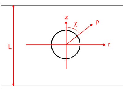
Figure 1: Illustration of the $(r,z)$ ”cylindrical” coordinates and the $(\rho,\chi)$ ”spherical” near horizon coordinates. The period of the compact dimension (in the $z$ direction) is denoted by $L$.

There is reason to expect good analytic control of small black holes even if we do not have a complete analytic solution since we have two good approximation in two different regions which overlap: for $\rho\ll L$ the metric is expected to resemble closely a $d$-dimensional Schwarzschild-Tangherlini BH [25], while for $\rho\gg\rho_{0}$ the gravitational field is weak and the newtonian approximation holds. Hence $\mu$ or more precisely $\rho_{0}/L\propto\mu^{1/d-3}$ is our small parameter for the perturbation.

The motivations for this research are first to obtain a theoretical description of this simple system which is important on its own right, and second to gain understanding of the phase transition physics through combination with numerical work. The symbiosis with numerical work comes close to serve as a partial substitute of experiments (which are sorely absent in this field): the numerics are essential for understanding big black holes close to the phase transition where the perturbative expansion is expected to break down, and the analytic control serves to formulate the aims and methods of the numerics. Moreover, the two can be used to test and confirm one another, as was the case for this research and [20, 21]. As it turns out the largest BH’s obtained numerically show only a single multipole mode correction to their spherical horizon [21, 22], and that lends some hope that the analytic expansion would retain some validity for large BH’s as well.

Basic set-up.

The first decision to be made it to choose the coordinates and ansatz for the analysis. At first one would hope to use a single coordinate patch for the whole metric. However, [18] showed that in the popular conformal coordinates (where the metric in the $(r,z)$ plane is in conformal form $ds^{2}=e^{2\hat{B}(r,z)}\,\left(dr^{2}+dz^{2}\right)$, see also below (111)) the coordinate size of the horizon is a conformal invariant and hence the coordinate patch necessarily changes with $\mu$. A similar phenomenon happens in the Harmark-Obers coordinates which are a semi-infinite cylinder with a single marked point [$(r,z)=(0,L/2)$] where the coordinate transformation is singular and whose location changes with $\mu$.

Therefore we choose to work with two coordinate patches (see figure 2): the near zone $\rho\ll L$ where the horizon ($\rho_{0}$) is fixed and the periodicity of $z$ is invisible far away, and the asymptotic zone $\rho\gg\rho_{0}$ where $L$ is fixed and $\rho_{0}$ is invisible. The metric in the two regions must be consistent over the overlap region $\rho_{0}\ll\rho\ll L$ (which grows indefinitely as $\mu\to 0$).

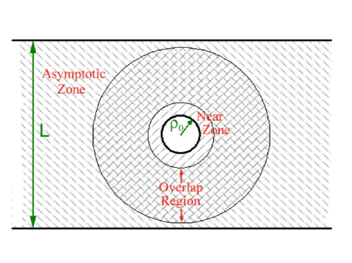
Figure 2: The division of the spacetime into two zones: the near zone $\rho\ll L$ where $\rho_{0}$ is fixed and the perturbative parameter is $L^{-1}$, and the asymptotic zone $\rho\gg\rho_{0}$ where $L$ is fixed and the perturbative parameter is $\rho_{0}$. The two zones overlap over the overlap region which increases indefinitely in the small black hole limit. During the perturbation process the two zones are separate, and communicate only through the matching “dialogue”. The near zone is defined by $\{(\rho,\chi):\,\rho\geq\rho_{0}\}$ while the asymptotic zone is defined by $\{(r,z):\,r\geq 0,~{}z\sim z+L\}\backslash(0,0)$.

Such a procedure is known in General Relativity as a “matched asymptotic expansion” — the metric is solved for in each asymptotic region and certain quantities are determined by matching the metrics over the overlap (for some recent examples see [26, 27, 28], in mathematical physics this idea goes back as far as Laplace who used it to find the shape of a drop of liquid on a surface — see [29] and references therein for a historical review). However, this is probably the first time such a procedure is used to find a static black hole solution.

We start by defining the domain for each zone and the zeroth order solution. In the near zone, whose domain is $\{(\rho,\chi):\,\rho\geq\rho_{0}\}$ we have a $d$-dimensional Schwarzschild black hole metric, with fixed $\rho_{0}$ and the perturbation is in orders of $L^{-1}$. In the asymptotic zone, on the other hand, the domain is $\{(r,z):\,r\geq 0,\,z\sim z+L\}\backslash(0,0)$, the zeroth order solution is simply the flat “cylinder” with the origin omitted, and the perturbation parameter is $\rho_{0}$.

Our objective is to describe the perturbation process (to any order) and apply it. The paper is organized as follows. In section 2 we describe the equations in the asymptotic zone and especially the newtonian potential. In section 3 we determine the linearized corrections to the Schwarzschild black hole in the near zone. In section 4 we describe the general perturbation procedure for this system and in 5 we present quantitative results on the leading corrections to the zeroth order metric. In the appendices we review some information on Heun’s equation and the Hypergeometric equation, review the definition of the surface gravity and give some details on vector harmonics in 5d (on ${\bf S}^{3}$). We now turn to the summary.

1.3 Summary

The asymptotic zone.

In section 2 we describe the asymptotic zone. The first correction to the zeroth order metrics described above is readily computed — it is the newtonian approximation in the asymptotic region (in standard harmonic gauge), where the newtonian potential (6) is obtained through the method of mirror images (considering the infinite sequence of sources in the covering space at $z=nL$ for any integer $n$). This term is proportional to $G_{N}\,M\propto\rho_{0}^{~{}d-3}$ and hence belongs to order $d-3$ in the asymptotic zone. Actually, the whole post-newtonian procedure is relevant and we review it, though in this paper all we need is the lowest order (newtonian) approximation.

Black hole perturbations.

The next correction to consider is the leading correction to the Schwarzschild solution. It is the analogue of the newtonian approximation only here the unperturbed background is curved, and it describes the response of the geometry to the mirror sources far away. Despite the analogy with the newtonian approximation the implementation is involved and is described in section 3.

In 4d this computation was carried out by Regge and Wheeler [30] who solved for all the linear perturbations, not only the static ones. Recently Ishibashi and Kodama succeeded to generalize their result to an arbitrary dimension, and to include a cosmological constant as well [31, 32, 33]. Our treatment is independent and we compare the two approaches below after describing our own.

The computation involves a few steps. We start by writing down the most general static perturbation to the metric. The spherical symmetry guarantees that at linear order perturbations in different representations of the rotation group will not mix, and we find by counting degrees of freedom that it suffices to consider “scalar harmonics” — representations which are the symmetric product of the vector representation, or equivalently, metric perturbations which are determined by scalar functions on the sphere. It turns out that the spherical symmetry also suggests a natural gauge which we term “no derivatives gauge” and completely fixes the reparameterization invariance, leaving us with 3 undetermined metric functions (fields).

Writing down the equations of motion and separating the angular variables we find that a Ricci flatness condition in the angular directions yields an algebraic relation among the radial functions (59) which is similar to a trace condition and allows us to eliminate one of the fields. After substitution one can express one of the remaining fields in terms of the other and its first and second derivatives. Performing the second substitution we are left with a second order ordinary differential equation (ODE), rather than a third or fourth order one would initially expect. So finally one has a single second order ODE in the radial direction, for one metric function (and for each spherical harmonic mode) from which the whole metric may be recovered. This is the so called “master equation” which after a change of variables simplifies further to become (75). It would be nice to have a deeper understanding why these reductions were to be expected.

The master equation belongs to the Heun class of Fuchsian equations, where Fuchsian means that the equation has only regular-singular points on the complex sphere which includes infinity, and Heun means that there are exactly 4 such points. Unlike the Hypergeometric case of 3 regular singularities there is no general solution to the Heun equation, though several methods are available. In this case however, it turns out that the solutions can be written in terms of a hypergeometric function, and it would be nice to understand why that had to be the case. Interestingly, we observe that in some of the relevant cases these hypergeometric functions simplify further to polynomials, and in particular in 5d all relevant solutions are polynomials (solutions which are of even multipole number and are regular at the horizon).

We started working out this problem before we were aware of the results of Kodama and Ishibashi [31, 32, 33] and we continued independently even after learning about these papers in order to avoid the formalism of gauge invariant perturbation theory, and the various changes of variables which are employed there. We were able to do so and actually found a somewhat different master (Heun) equation. Yet the final reduction of our master Heun equation to a hypergeometric one was motivated by those papers.

The matching procedure.

One of the main results of this paper is the construction of a perturbation method for the metric (in both patches) which may be carried in principle to an arbitrarily high order in the small parameter. The method is described in section 4. A crucial step is to identify a dimensionful expansion parameter on each patch: $\rho_{0}$ in the asymptotic zone and $L^{-1}$ in the near region. As in any perturbative expansion, at each order one needs to solve a non-homogenous linear equation — the linear equation being the same as the one which appears at first order and the non-homogeneous source term being constructed from lower order metric functions. The precise form of the source term depends on the higher order gauge choice which we do not specify, but will not change the method we describe. The solution to this equation is determined up to a solution of the homogeneous equation. This indeterminacy for each zone on its own reflects the freedom of adding external field multipoles — in the asymptotic zone they are situated at the origin while in the near zone they are at infinity. These external multipoles must be determined by matching with the other zone, a procedure which requires to identify (after matching the gauge) the leading terms in the metric on both zones. We call this process “a dialogue of multipoles”.

A priori it is not obvious that the required terms from the other zone are already available at the right time, namely that the method is well-posed (that there are sufficient boundary conditions). Hence it is interesting to study at any given order in a specific zone which orders must be already available for matching from the other one, and thereby describe the pattern of the dialogue — the orders at which one should alternate between the zones. This pattern can be determined by a simple dimensional analysis of the multipole coefficients as we describe in the text, and indeed we find the system to be well-posed. Interestingly, the dialogue pattern which emanates is dimension dependent: 5d is special in that one scales a single order in the perturbation ladder on each zone and then alternates to the other zone; for $d>5$ one needs to climb several steps before going to the other zone, and in the $d\to\infty$ limit one gets infinitely many constants already from matching with the newtonian potential alone.

Quantitative matching results.

In section 5 we apply the general procedure to the leading order and match the newtonian potential at the asymptotic zone to get the leading correction to the Schwarzschild solution in the near zone. To this purpose it is essential to have available certain matching constants which can be read from the explicit solutions we derived for the linear perturbations of Schwarzschild. The next order correction is currently under study [34].

¿From the metric which we obtain one may extract certain “measurables”:

• The leading correction to the mass — temperature relation is given in (97). At this order the BH is still spherical but there is a correction to this relation since the small black hole does not asymptote in the near zone to flat space with zero potential, but rather there is a non-zero potential shift due to the images.

• The leading (quadrupole) departure from a spherical horizon — measured by the “eccentricity” is given in (110). The result of the deformation is to make the black hole longer along the $z$ axis compared to the $r$ axis as in figure 9 and can be understood from the shape of small (newtonian) equipotential lines around $\rho=0$ (see figure 3).

• The coefficient of the “inter-polar distance” is given in (122). By “inter-polar” distance we mean the proper distance from the “north pole” of the black hole around the compact circle and up to the “south pole”(see figure 11). Actually the black hole tends to “make room” for itself, in the sense that the inter-polar distance added to the black hole size in conformal coordinates is always larger than $L$, the size of the compact dimension. This can be re-stated as the observation that such black holes seem to always have a positive scalar charge as seen from infinity similar to the ordinary positive mass theorem (where the scalar is the one which arises from the dimensional reduction of the $g_{zz}$ metric component — the size of the extra dimension). In 5d the effect is the strongest, where to leading order in the small parameter the inter-polar distance does not decrease at all. We term that “a black hole Archimedes effect” since the black hole repels or expands an amount of space equal to its size in 5d (and less in higher dimensions).

Most of these results were already announced in [20] and here we add the determination of the inter-polar distance and the generalization of the eccentricity for $d>5$. They were numerically confirmed in 5d [21] as well as in 6d [35, 36] and other dimensions [36]. Recently a paper [23] has appeared deriving the leading order form of the metric within the framework of the Harmark-Obers coordinates [11], and as such overlaps with the results announced in [20] and proven here. The overlap includes the corrections to the temperature and area, while [23] obtains also the corrections to the mass and tension, and this paper derives the eccentricity and “Archimedes effect”. Moreover, here we go beyond and demonstrate a method for an arbitrary number of successive approximations.

Note added: In the 3rd version we performed some rewriting of subsection 3.3.2 where we made minor corrections and improved the clarity and we corrected a trivial factor of 2 in (125).

2 The asymptotic zone

In this section we write the static Einstein equations in a form that will be convenient for iterative expansion in a small parameter around the flat Minkowsky spacetime. This type of expansion is known as “post-newtonian expansion” (see [29]) and we follow here the usual conventions for this type of expansion. The leading order in the expansion is the newtonian approximation. We repeat here the calculation of the newtonian approximation for the caged black hole which appeared in many places (see for example [11, 23]). The following orders in the expansion are called “post-newtonian” and their calculation will appear in [34].

For the post-newtonian expansion it is convenient to write the Ricci tensor in the following form [37]

$$R_{\mu\nu}=-\frac{1}{2}g_{\mu\sigma}g_{\nu\rho}g^{\alpha\beta}\frac{\partial^{2}g^{\rho\sigma}}{\partial x^{\alpha}\partial x^{\beta}}+\Gamma_{\mu}^{\alpha\beta}\Gamma_{\nu,\alpha\beta}-\Gamma_{\mu\nu},$$ (1)

where $\Gamma_{\mu,\alpha\beta}$ and $\Gamma_{\mu}^{\alpha\beta}$ are the Christoffel symbols of the first and the second kind, respectively, and in addition one defines

$$\Gamma_{\mu\nu} \equiv \frac{1}{2}\bigg{(}g_{\mu\rho}\frac{\partial\Gamma^{\rho}}{\partial x^{\nu}}+g_{\nu\sigma}\frac{\partial\Gamma^{\sigma}}{\partial x^{\mu}}-g_{\mu\rho}g_{\nu\sigma}\frac{\partial g^{\rho\sigma}}{\partial x^{\alpha}}\Gamma^{\alpha}\bigg{)}\,,$$

$$\Gamma^{\nu} \equiv g^{\alpha\beta}\Gamma^{\nu}_{\alpha\beta}\,.$$

Next one chooses the harmonic (or de Donder ) gauge by the requirement that

$$\Gamma^{\nu}=\Box x^{\nu}=\frac{1}{\sqrt{-g}}\frac{\partial}{\partial x^{\beta}}(\sqrt{-g}g^{\beta\nu})\equiv 0\,.$$ (2)

where we denote by $g$ the determinant of the metric $g_{\mu\nu}$. In this gauge, the last term in the expression of the Ricci tensor above vanishes. This choice of gauge is very convenient for expansion in the asymptotic zone. Finally one attempts to solve Einstein’s equations.

The first step in this iterative procedure is to look at the linearized equations valid for weakly gravitating regions, namely making the newtonian approximation. The metric is taken to be

$$g_{\mu\nu}=\eta_{\mu\nu}+h_{\mu\nu}\,.$$ (3)

The harmonic gauge equation (2) takes the more famous form (for example in the treatment of gravitational waves)

$$\left(h_{\mu\nu}-\frac{1}{2}h^{\alpha}_{\alpha}\,\eta^{\mu\nu}\right)_{,\nu}=0\,.$$

One defines

$$\bar{h}_{\mu\nu}\equiv h_{\mu\nu}-\frac{1}{2}h^{\alpha}_{\alpha}\,\eta_{\mu\nu}\,,$$ (4)

in terms of which the linearized field equations become

$$\frac{1}{2}\,\Box\bar{h}_{\mu\nu}=G_{\mu\nu}=8\pi\,G_{d}\,T_{\mu\nu}\,,$$ (5)

where $\Box$ is the flat space D’alambertian.

In our case, working on the covering space implies an infinite array of newtonian sources in the $z$ direction and the only non-zero components of the energy momentum tensor is

$$T_{00}=\sum_{n=-\infty}^{\infty}M\,\delta^{d-2}(x_{1},\dots,x_{d-2})\,\delta(z-nL)\,,$$

where $(x_{1},\dots,x_{d-2})$ denote the extended spatial coordinates. The method of images can be used to solve the equation for $\bar{h}_{00}$

$$\bar{h}_{00}=-{\Phi_{N}\over 4\pi} \equiv \frac{16\,\pi\,G_{d}\,M}{(d-3)\,\Omega_{d-2}}\sum_{n=-\infty}^{\infty}\frac{1}{\left(r^{2}+(z+nL)^{2}\right)^{\frac{d-3}{2}}}=$$ (6)

$$= {d-2\over d-3}\,\rho_{0}^{d-3}\,\sum_{n=-\infty}^{\infty}\frac{1}{\left(r^{2}+(z+nL)^{2}\right)^{\frac{d-3}{2}}}\,,$$

where $\Phi_{N}$ is the newtonian potential, conventionally normalized such that its flux through a surface enclosing a mass $M$ is $4\pi\,G_{d}\,M$, $\rho_{0}$ is given by [39]

$$\rho_{0}^{d-3}=\frac{16\,\pi\,G_{d}\,M}{(d-2)\,\Omega_{d-2}}\,,$$ (7)

and

$$\Omega_{d-2}=\frac{2\,\pi^{\frac{d-1}{2}}}{\Gamma(\frac{d-1}{2})}\,,$$

is the area of a unit $S^{d-2}$. A more formal alternative to obtain the prefactor of the newtonian potential in equation (6) is through matching with the Schwarzschild metric in the near zone.

We see that the first correction to the metric in the asymptotic region is of order $\rho_{0}^{~{}d-3}$. We will see later that we must choose the perturbation parameter in this region to be $\rho_{0}$ rather than $\rho_{0}^{~{}d-3}$, namely

$$g_{\mu\nu}=\sum_{n=0}^{\infty}\rho_{0}^{~{}n}\,g_{\mu\nu}^{(n)}\,,$$ (8)

and hence we see that the leading correction comes at order $d-3$, namely

$$g^{(0)}_{\mu\nu} = \eta_{\mu\nu}\,,$$

$$g^{(d-3)}_{\mu\nu} = h_{\mu\nu}\,.$$ (9)

Transforming back to $h_{\mu\nu}$ using the inverse of (4)

$$h_{\mu\nu}\equiv\bar{h}_{\mu\nu}-\frac{1}{d-2}\bar{h}^{\alpha}_{\alpha}\,\eta_{\mu\nu}\,,$$ (10)

yields the expression for the metric perturbation in terms of the newtonian potential (6)

$$h_{00} = -{d-3\over d-2}{\Phi_{N}\over 4\pi}=\rho_{0}^{d-3}\sum_{n=-\infty}^{\infty}\frac{1}{\left(r^{2}+(z+nL)^{2}\right)^{\frac{d-3}{2}}},$$

$$h_{ij} = -{1\over d-2}{\Phi_{N}\over 4\pi}\,\delta_{ij}={1\over d-3}\,h_{00}\,\delta_{ij}\,,$$ (11)

where the Latin indices stand for the spatial components.

In the 5d case one can express the newtonian potential as

$$\Phi=-\frac{G_{5}\,M}{L\,r}\cdot\frac{\sinh\left(\frac{2\,\pi\,r}{L}\right)}{\cosh\left(\frac{2\,\pi\,r}{L}\right)-\cos\left(\frac{2\,\pi\,z}{L}\right)}\,.$$ (12)

In figure 3 we give the equipotential surfaces of the newtonian potential in 5d, and they look qualitatively the same in any dimension $d>5$.

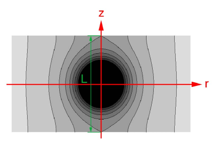
Figure 3: Equipotential surfaces of the newtonian potential in 5d.

We close this section with two comments. First, at higher orders in the perturbation procedure the form of the equations is dominated by the linearized equations and is given by

$$\Box g^{(m),\mu\nu}=\it{F}(g,\partial g)\,,$$

where $(m)$ is the order under study and $\it{F}(g,\partial g)$ are source terms which are quadratic, at least, in lower order metric components and their derivatives. The second remark is that in this section all the expressions for the metric components were in the harmonic gauge. In the next sections we use the Schwarzschild gauge in the near zone. To avoid cluttering the notation we will not introduce always a different letter for every gauge — in subsection 4.1 we give different notation for $\rho$ in the two gauges ($\rho$ in the Schwarzschild coordinates and $\rho_{h}$ in the harmonic gauge) but later we omit the difference in the notation. However, it is important to remember the difference in the gauge between the two zones.

3 Black hole perturbations

As explained in the introduction the zeroth order in the near (horizon) zone is the $d$-dimensional Schwarzschild-Tangherlini metric [25]

$$ds^{2}=-f(\rho)\,dt^{2}+\frac{1}{f(\rho)}\,d\rho^{2}+\rho^{2}\,d\Omega_{d-2}^{2}\,,$$

where $f(\rho)=1-\frac{\rho_{0}^{d-3}}{\rho^{d-3}}$, $\rho_{0}$ is related to $M$ via (7) and

$$d\Omega_{d-2}^{2}=d\chi^{2}+\sin^{2}\chi\,d\theta_{1}^{2}+\cdots+(\sin^{2}\chi\,\sin^{2}\theta_{1}\ldots\sin^{2}\theta_{d-4})\,d\theta_{d-3}^{2}\,,$$

is the metric on $S^{d-2}$.

In this section we find the linear static perturbations for the $d$-dimensional Schwarzschild solution. Regge and Wheeler [30] derived the linear equations that describe small perturbations to the four dimensional Schwarzschild black hole, and here we generalize their method for the static case. These perturbations can be interpreted as deviations of the black hole from spherical symmetry due to remote masses. In the case of a compact dimension, we are interested in the influence of the black hole (images) on itself. Therefore we assume that the $\mathop{\rm SO}\nolimits(d-2)$ symmetry in the spherical coordinates $(\theta_{1},\ldots,\theta_{d-3})$ is still preserved and the deformation of the black hole takes place only in the $(\rho,\chi)$ plane (which in “cylindrical” coordinates will be part of the $(r,z)$ plane). We denote in this section the $d$-dimensional Schwarzschild metric by $g_{\mu\nu}$ and the perturbation metric by $h_{\mu\nu}$. Therefore, $h_{\mu\nu}$ is a function only of $\rho$ and $\chi$.

The linearized vacuum Einstein equations can be brought to the simplified form [40]

$$\delta R_{\mu\nu}=-\frac{1}{2}D_{\mu}D_{\nu}h-\frac{1}{2}D^{\sigma}D_{\sigma}h_{\mu\nu}+D^{\sigma}D_{(\nu}h_{\mu)\sigma}=0\,,$$ (13)

where $h=g^{\mu\nu}h_{\mu\nu}$, $D^{\mu}$ is the covariant derivative with respect to the background metric $g_{\mu\nu}$ and $A_{(\alpha\beta)}\equiv\left(A_{\alpha\beta}+A_{\beta\alpha}\right)/2$ stands for the symmetric part of a tensor $A_{\alpha\beta}$.

3.1 Spherical harmonics on ${\bf S}^{d-2}$

Our goal is to simplify the equations by reducing them to a system of ordinary differential equations. Following Regge and Wheeler we start by expanding the solution, $h_{\mu\nu}$, into generalized spherical harmonics on the sphere $S^{d-2}$. Each component of $h_{\mu\nu}$ is transformed under local coordinate changes of $S^{d-2}$ like a scalar, a vector or a tensor. Hence, we decompose $h_{\mu\nu}$ into 3 types of spherical harmonics: scalar, vector and tensor harmonics. The scalar components are: $h_{tt}$, $h_{\rho\rho}$ and $h_{\rho t}$. The vectors are: $(h_{t\chi},h_{t\theta_{1}},\ldots,h_{t\theta_{d-3}})$ and $(h_{\rho\chi},h_{\rho\theta_{1}},\ldots,h_{\rho\theta_{d-3}})$. The tensor is formed of the block

$$\left(\begin{array}[]{ccccc}h_{\chi\chi}&h_{\chi\theta_{1}}&h_{\chi\theta_{2}}&\cdots&h_{\chi\theta_{d-3}}\\ *&h_{\theta_{1}\theta_{1}}&h_{\theta_{1}\theta_{2}}&\cdots&h_{\theta_{1}\theta_{d-3}}\\ *&*&h_{\theta_{2}\theta_{2}}&\cdots&h_{\theta_{2}\theta_{d-3}}\\ \vdots&\vdots&\vdots&\ddots&\vdots\\ *&*&*&\cdots&h_{\theta_{d-3}\theta_{d-3}}\end{array}\right),$$

where we denote by $*$ symmetric components. Counting degrees of freedom we find that we should have 3 elements in the basis of the scalar harmonics, $2\,(d-2)$ in the basis of the vector harmonics and $\frac{(d-2)\,(d-1)}{2}$ in the basis of the tensor harmonics. Together we obtain all the $\frac{d\,(d+1)}{2}$ components of $h_{\mu\nu}$.

Since we are interested in expansion to harmonics which are static and have $\mathop{\rm SO}\nolimits(d-2)$ symmetry the non-vanishing components of the tensor $h_{\mu\nu}$ are:

$$\left(\begin{array}[]{cccccc}h_{tt}&&&&&\\ &h_{\rho\rho}&h_{\rho\chi}&&&\\ &*&h_{\chi\chi}&&&\\ &&&h_{\theta_{1}\theta_{1}}&&\\ &&&&\ddots&\\ &&&&&h_{\theta_{d-3}\theta_{d-3}}\end{array}\right),$$ (14)

where in addition, the $\mathop{\rm SO}\nolimits(d-2)$ symmetry implies that the only independent angular components on the diagonal are $h_{\chi\chi}$ and $h_{\theta_{1}\theta_{1}}$. The rest of the angular components are obtained through the relations

$$h_{\theta_{i}\theta_{i}}=\sin^{2}{\theta_{i-1}}\,h_{\theta_{i-1}\theta_{i-1}}\,,\qquad i=2,\ldots,d-3\,.$$

Note that there are only 5 independent components of $h_{\mu\nu}$, namely $h_{tt}$, $h_{\rho\rho}$, $h_{\rho\chi}$, $h_{\chi\chi}$, $h_{\theta_{1}\theta_{1}}$, comprising of 2 scalars, 1 vector and 2 tensors, and these numbers are independent of the dimension. Accordingly, we will find 5 linear ordinary differential equations (the equations of motion).

3.1.1 Scalar harmonics

By considering the flat $(d-1)$-dimensional Laplace equation we can get both the scalar spherical harmonics on ${\bf S}^{d-2}$, and the leading radial profile of the multipoles in the nearly flat region $\rho\gg\rho_{0}$. Since we assume $\mathop{\rm SO}\nolimits(d-2)$ symmetry we consider a Laplace equation for a function which depends only on one angular variable $\chi$. Thus, the Laplace equation for a function $\Psi(\rho,\chi)$ on $\mathbb{R}^{d-1}$ would be

$$\partial_{\rho}\left(\rho^{d-2}\,\sin^{(d-3)}(\chi)\,\partial_{\rho}\Psi(\rho,\chi)\right)+\rho^{d-4}\,\partial_{\chi}\left(\sin^{(d-3)}(\chi)\,\partial_{\chi}\Psi(\rho,\chi)\right)=0\,.$$ (15)

Separation of variables $\Psi(\rho,\chi)=R(\rho)\,\Pi(\chi)$ gives us two separated equations for each eigenvalue $l$ which denotes also the number of the multipole in the expansion

$$\Psi(\rho,\chi)=\sum_{l=0}^{\infty}R_{l}(\rho)\,\Pi^{l,d}_{0}(\chi)\,.$$

$\Pi^{l,d}_{0}(\chi)$ is the angular function which is associated with each one of the multipoles. The extra zero index in the angular function stands to remind us that had we not had the $\mathop{\rm SO}\nolimits(d-2)$ symmetry, the angular functions, which depends on $\chi$, would have additional indices (additional “quantum numbers”). (For an example see the 5d case later in this subsection). The equation for $\Pi^{l,d}_{0}(\chi)$ is

$$\frac{d^{2}\,\Pi^{l,d}_{0}}{d\chi^{2}}+(d-3)\,\cot(\chi)\frac{d\,\Pi^{l,d}_{0}}{d\chi}+l\,(l+d-3)\,\Pi^{l,d}_{0}=0\,,$$ (16)

where $l\,(l+d-3)$ are the eigenvalues. This equation can be brought to the form of a Legendre equation [41] in $d-1$ dimensions using the substitution $t=\cos(\chi)$ (then the solutions of the equation are called Legendre polynomials of the variable $t$ in $d-1$ dimensions). The solutions can be expressed by a Rodriguez formula (see [41])

$$\Pi^{l,d}_{0}(\chi)=\frac{\Gamma(\frac{d}{2}-1)}{2^{l}\,\Gamma(l+\frac{d}{2}-1)}\,\sin^{4-d}(\chi)\,\left(\frac{1}{\sin(\chi)}\,\frac{d}{d\chi}\right)^{l}\,\sin^{2l+d-4}(\chi)\,,$$ (17)

where the prefactor with the Gamma functions fixes the usual normalization of the Legendre polynomials.

The functions $R_{l}(\rho)$ give us the radial part of the expansion. $R_{l}(\rho)$ is obtained as the solution of the eigenvalue equation

$$\frac{d}{d\rho}\left(\rho^{d-2}\,R_{l}\,^{\prime}(\rho)\right)-l\,(l+d-3)\,\rho^{d-4}\,R_{l}(\rho)=0\,.$$ (18)

Therefore

$$R_{l}(\rho)=J_{l}\,\rho^{-(l+d-3)}+K_{l}\,\rho^{l}\,,$$ (19)

where $J_{l}$ and $K_{l}$ are constants. For fixed $l$ and $d$ the first term is the multipole of a mass distribution at $\rho=0$ and the second term is the multipole of a mass distribution at infinity. Note that $l=0$ is the first multipole — the monopole, $l=1$ is the dipole and so on.

Since the linear equations for $h_{\mu\nu}$ (13) are $\mathop{\rm SO}\nolimits(d-1)$ invariant we may separate the angular variables, and since the perturbed metric depends only on $(\rho,\chi)$, we may expand the scalar components $h_{tt}$ and $h_{\rho\rho}$ in spherical harmonics as follows

$$h_{tt} = \sum_{l=0}^{\infty}\tilde{A_{l}}(\rho)\,\Pi^{l,d}_{0}(\chi)\,,$$

$$h_{\rho\rho} = \sum_{l=0}^{\infty}\tilde{B_{l}}(\rho)\,\Pi^{l,d}_{0}(\chi)\,,$$ (20)

where the radial functions $\tilde{A_{l}}(\rho),\,\tilde{B_{l}}(\rho)$ satisfy some differential equations to be discussed later.

5d scalar spherical harmonics.

As a concrete simple example, where we can give explicit formulae for the scalar harmonics, let us consider the 5d case. Gerlach and Sengupta used this type of decomposition in 5d for the Robertson-Walker spacetime [42]. Let us denote the scalar spherical harmonics in 5 dimensions by $Q^{n}_{lm}(\chi,\theta,\varphi)$. They can be separated into a product of two types of functions

$$Q^{n}_{lm}(\chi,\theta,\varphi)=\Pi^{n,5}_{l}(\chi)\,Y_{lm}(\theta,\varphi)\,,$$

where $Y_{lm}(\theta,\varphi)$ are the usual spherical harmonics on $S^{2}$ and $\Pi^{n,5}_{l}(\chi)$ are the “Fock” harmonics (see [42, 43]), which are given by

$$\Pi^{n,5}_{l}(\chi)=\sin^{l}(\chi)\,\frac{d^{l+1}\,(\cos((n+1)\,\chi))}{d(\cos(\chi))^{l+1}}\,.$$

Since we require $\mathop{\rm SO}\nolimits(3)$ symmetry for the $(\theta,\varphi)$ two-sphere, we take $l=m=0$ in the spherical harmonics. Thus we arrive to (16) in the 5d case (with the index $n$ instead of $l$)

$$\frac{d^{2}\,\Pi^{n,5}_{0}}{d\chi^{2}}+2\,\cot(\chi)\,\frac{d\,\Pi^{n,5}_{0}}{d\chi}+n\,(n+2)\,\Pi^{n,5}_{0}=0\,,$$ (21)

whose solutions are Chebyshev polynomials of the second kind

$$\Pi^{n,5}_{0}(\chi)=\frac{\sin[(n+1)\,\chi]}{\sin(\chi)}\equiv U_{n}(\cos(\chi))\,.$$

3.1.2 Vector and tensor harmonics

Given a family of scalar harmonics one can form a family of “scalar derived” vector harmonics simply by taking its gradient. There are other, more involved, vector harmonics as well, but we shall see now that the “scalar derived” family suffices for our purposes. For a concrete example of a basis of vector harmonics in 5d (on ${\bf S}^{3}$) see appendix C.

Due to the symmetries the vector has a single component (14)

$$h_{\rho\mu}=h_{\rho\chi}(\rho,\chi)\,\delta_{\mu\chi}\,,$$ (22)

where $\mu$ runs over the angular coordinates only. Denoting $\hat{h}(\rho,\chi)\equiv\int^{\chi}d\chi^{\prime}\,h_{\rho\chi}(\rho,\chi^{\prime})$ we have

$$h_{\rho\mu}={\partial}_{\mu}\hat{h}(\rho,\chi)\,.$$ (23)

Therefore, after expanding $\hat{h}$ into spherical harmonics and substituting in (23) we can write the expansion of $h_{\rho\chi}$ into radial functions $\tilde{C_{l}}(\rho)$ as

$$h_{\rho\chi}=\sum_{l=0}^{\infty}\tilde{C_{l}}(\rho)\,{\partial}_{\chi}\Pi^{l,d}_{0}(\chi)\,.$$ (24)

A similar argument holds for the tensor components which are essentially $h_{\chi\chi}$, $h_{\theta_{1},\theta_{1}}$ (14). Again there are exactly two “scalar derived” tensor harmonics

$$\hat{D_{i}}\hat{D_{j}}\Pi^{l,d}_{0}\,,$$ (25)

and

$$\gamma_{ij}\,\Pi^{l,d}_{0}\,,$$ (26)

where $\gamma_{ij}$ is the metric on the sphere $S^{d-2}$, $\hat{D_{i}}$ is the covariant derivative on $S^{d-2}$, and the second term is proportional to the trace of the first. So we have two tensor harmonics to decompose into, which is exactly the number we need, and indeed one can verify that these two families always suffice.

Hence we can decompose the tensor part into radial functions $\tilde{D_{l}}(\rho)$, $\tilde{E_{l}}(\rho)$

$$\sum_{l=0}^{\infty}\tilde{D_{l}}(\rho)\left(\begin{array}[]{cccc}\frac{\partial^{2}}{\partial\chi^{2}}&&&\\ &\sin(\chi)\cos(\chi)\frac{\partial}{\partial\chi}&0&\\ &&\sin(\chi)\cos(\chi)\sin^{2}(\theta_{1})\frac{\partial}{\partial\chi}&\\ &&&\ddots\end{array}\right)\Pi^{l,d}_{0}(\chi)+$$ (31)

$$+\sum_{l=0}^{\infty}\tilde{E_{l}}(\rho)\left(\begin{array}[]{cccc}1&&&\\ &\sin^{2}(\chi)&&\\ &&\sin^{2}(\chi)\sin^{2}(\theta_{1})&\\ &&&\ddots\end{array}\right)\Pi^{l,d}_{0}(\chi)\,.$$ (36)

The discussion above led us to the conclusion that the only elements of both the vector and tensor basis which survived under our symmetry requirements are the “scalar derived” ones. These are in the “scalar type” representation under the $\mathop{\rm SO}\nolimits(d-1)$ rotation group, where by “scalar type” we mean representations whose Dynkin indices are $[l,0,\dots,0]$ for some $l\geq 0$, namely those in the $l$-times traceless symmetric product of the vector representation. More generally, Kodama and Sasaki [44] pointed out that one can classify the different basis elements into three groups with respect to their different representations under the rotation isometry group: scalar, vector and tensor “type”. This classification into representations of the isometry group should not be confused with the classification that we used above with respect to local coordinate transformations of $S^{d-2}$. So, according to this classification, (24) is a vector of “scalar type” under the rotation group and (36) is a tensor of “scalar type” as well. Since we deal with linear equations two different representations cannot mix. Thus even if there were any representations of non-scalar “type” in the decomposition of the perturbed metric, they would not appear in the equations for the scalar type radial functions $\tilde{A_{l}},\,\tilde{B_{l}},\,\tilde{C_{l}},\,\tilde{D_{l}},\,\tilde{E_{l}}$.

3.2 The choice of gauge

We have now 5 radial fields ($\tilde{A_{l}}(\rho)$,..,$\tilde{E_{l}}(\rho)$) defined in (20), (24), (36) for each mode of the expansion. We can reduce further the number of fields to 3 using the gauge freedom. The gauge transformations of linearized general relativity about a solution $g_{\mu\nu}$ are of the form

$$h_{\mu\nu}\longrightarrow h_{\mu\nu}+D_{\nu}\xi_{\mu}+D_{\mu}\xi_{\nu}\,,$$

where $\xi^{\mu}$ is an arbitrary vector field — the generator of an infinitesimal transformation. The most general generator consistent with the symmetries is

$$\xi_{t} = 0\,,$$

$$\xi_{\rho} = \sum_{l=0}^{\infty}L_{l}(\rho)\,\Pi^{l,d}_{0}(\chi)\,,$$

$$\xi_{\chi} = \sum_{l=0}^{\infty}M_{l}(\rho)\,\Pi^{l,d\prime}_{0}(\chi)\,,$$

$$\xi_{\theta_{1}} = 0,\ldots,\xi_{\theta_{d-3}}=0\,.$$ (37)

It is natural to eliminate the “scalar derived” functions $\tilde{C_{l}}(\rho)$ and $\tilde{D_{l}}(\rho)$ in each mode, putting $h_{\mu\nu}$ in a diagonal form. We term this the “no derivative gauge”. Thus,

$$h_{\rho\chi} \longrightarrow h_{\rho\chi}+D_{\chi}\xi_{\rho}+D_{\rho}\xi_{\chi}$$

$$= h_{\rho\chi}+\xi_{\rho,\chi}+\xi_{\chi,\rho}-2\,\Gamma_{\rho\chi}^{\chi}\,\xi_{\chi}$$

$$= \sum_{l=0}^{\infty}\left(\tilde{C_{l}}+L_{l}+M_{l}^{\prime}-\frac{2}{\rho}\,M_{l}\right)\,\Pi^{l,d\prime}_{0}(\chi)\,,$$

$$h_{\chi\chi} \longrightarrow h_{\chi\chi}+2\,D_{\chi}\xi_{\chi}$$

$$= h_{\chi\chi}+2\,\xi_{\chi,\chi}-2\,\Gamma_{\chi\chi}^{\rho}\,\xi_{\rho}$$

$$= \sum_{l=0}^{\infty}\left(\tilde{E_{l}}+2\,\rho\,f\,L_{l}\right)\,\Pi^{l,d}_{0}(\chi)+\left(\tilde{D_{l}}+2\,M_{l}\right)\Pi^{l,d\prime\prime}_{0}(\chi)\,.$$

The required gauge implies that the functions $L_{l}(\rho)$ and $M_{l}(\rho)$ should satisfy the following conditions

$$\tilde{C_{l}}+L_{l}+M_{l}^{\prime}-\frac{2}{\rho}\,M_{l} = 0\,,$$

$$\tilde{D_{l}}+2\,M_{l} = 0\,.$$ (38)

Moreover, since $\tilde{E_{l}}$ is arbitrary function of $\rho$ we can redefine it using the transformation $\tilde{E_{l}}\rightarrow\tilde{E_{l}}+2\,\rho\,f\,L_{l}$. These equations for $L_{l}(\rho)$ and $M_{l}(\rho)$, although including differential operators, are actually algebraic and have a single solution (for each mode) without any additional gauge freedom, i.e., the gauge is completely fixed. Applying the gauge transformation to any component of ($h_{\theta_{1}\theta_{1}}$,…,$h_{\theta_{d-3}\theta_{d-3}}$) yields the same equations as in the case of $h_{\chi\chi}$ using (16).

3.3 The field equations

3.3.1 The master equation

After gauge fixing the perturbed metric diagonalizes and we are left with 3 metric functions $h_{tt},\,h_{\rho\rho},\,h_{\chi\chi}$, which are functions of $(\rho,\chi)$

$$h_{\mu\nu}\,dx^{\mu}\,dx^{\nu} = \tilde{A}(\rho,\chi)\,dt^{2}+\tilde{B}(\rho,\chi)\,d\rho^{2}+\tilde{E}(\rho,\chi)\,d\Omega_{d-2}^{~{}2}$$ (39)

$$= \sum_{l=0}^{\infty}\left(\tilde{A_{l}}(\rho)\,dt^{2}+\tilde{B_{l}}(\rho)\,d\rho^{2}+\tilde{E_{l}}(\rho)d\Omega_{d-2}^{~{}2}\right)\Pi^{l,d}_{0}(\chi)\,.$$

It turns out that Einstein’s equations simplify if we use $h^{\mu}_{~{}\nu}$ instead of $h_{\mu\nu}$. Thus we define $A\equiv-\frac{\tilde{A}}{f}$, $B\equiv f\,\tilde{B}$, $E\equiv\frac{\tilde{E}}{\rho^{2}}$ where as usual $f(\rho)=1-\frac{\rho_{0}^{d-3}}{\rho^{d-3}}$. The ansatz in the new variables reads

$$h^{\mu}_{~{}\nu} = \left(\begin{array}[]{ccccc}A(\rho,\chi)&&&&\\ &B(\rho,\chi)&&&\\ &&E(\rho,\chi)&&\\ &&&\ddots&\\ &&&&E(\rho,\chi)\ldots\end{array}\right)$$ (45)

$$= \sum_{l=0}^{\infty}\left(\begin{array}[]{ccccc}A_{l}(\rho)&&&&\\ &B_{l}(\rho)&&&\\ &&E_{l}(\rho)&&\\ &&&\ddots&\\ &&&&E_{l}(\rho)\ldots\end{array}\right)\Pi^{l,d}_{0}(\chi)\,.$$ (51)

We substitute this ansatz into the linearized Einstein equations, (13) and using (16) we obtain, as expected, five equations

$\delta R_{tt}=0;$

$$2\,l\,(l+d-3)\,A_{l}-(3\,\rho^{2}\,f^{\prime}+2\,(d-2)\rho\,f)\,A_{l}^{\prime}+\rho^{2}\,f^{\prime}\,B_{l}^{\prime}-(d-2)\,\rho^{2}\,f^{\prime}\,E_{l}^{\prime}-2\,\rho^{2}\,f\,A_{l}^{\prime\prime}=0\,,$$ (52)

$\delta R_{\rho\rho}=0;$

$$2\,l\,(l+d-3)\,B_{l}-3\,\rho^{2}\,f^{\prime}\,A_{l}^{\prime}+2\,(d-2)\,\rho f\,{B}^{\prime}_{l}+\rho^{2}\,f^{\prime}\,B_{l}^{\prime}-$$

$$-4\,(d-2)\,\rho\,f\,E_{l}^{\prime}-(d-2)\,\rho^{2}\,f^{\prime}\,E_{l}^{\prime}+2\,\rho^{2}\,f\,A_{l}^{\prime\prime}-2\,(d-2)\,\rho^{2}\,f\,E_{l}^{\prime\prime} = 0\,,$$ (53)

$\delta R_{\rho\chi}=0;$

$$-(\rho\,f^{\prime}-2\,f)\,A_{l}+2\,(d-3)\,f\,B_{l}+\rho\,f^{\prime}\,B_{l}-2\,\rho\,f\,A_{l}^{\prime}-2\,(d-3)\,\rho\,f\,E_{l}^{\prime}=0\,,$$ (54)

$\delta R_{\chi\chi}=0;$

$$-b_{l}(\rho)\,\Pi^{l,d}_{0}(\chi)-\frac{1}{2}\,a_{l}(\rho)\,\Pi^{l,d\prime\prime}_{0}(\chi)=0\,,$$ (55)

$\frac{\delta R_{\theta\theta}}{\sin^{2}(\chi)}-\delta R_{\chi\chi}=0;$

$$-\frac{1}{2}\,a_{l}(\rho)\,\left(\cot(\chi)\,\Pi^{l,d\prime}_{0}(\chi)-\Pi^{l,d\prime\prime}_{0}(\chi)\right)=0\,,$$ (56)

where we define

$$a(\rho) \equiv A+B+(d-4)\,E=\mbox{tr}(h)-2E\,,$$

$$a(\rho) = \sum_{l=0}^{\infty}\,a_{l}(\rho)\,\Pi^{l,d}_{0}(\chi)\,,$$ (57)

$$b_{l}(\rho) \equiv (d-3)\,(E_{l}-B_{l})+\frac{1}{2}\,\rho\,f\,(A_{l}^{\prime}-B_{l}^{\prime})+\frac{1}{2}\,\rho^{2}\,f^{\prime}\,(E_{l}^{\prime}+E_{l}^{\prime\prime})+$$ (58)

$$+(d-2)\,\rho\,f\,E_{l}^{\prime}-\frac{1}{2}\,l\,(l+d-3)\,E_{l}\,.$$

Three of the equations are second order in the derivatives. These are the evolution equations. One of the equations is first order ($\delta R_{\rho\chi}=0$) — the constraint equation. For $l>0$ the expression in the brackets in (56) is non-zero and we get the following algebraic relation

$$\framebox{$~{}\rule[-5.69054pt]{0.0pt}{22.76219pt}\displaystyle a_{l}(\rho)=A_{l}+B_{l}+(d-4)\,E_{l}=0\,.$}$$ (59)

The case $l=0$ is degenerate and we will discuss it separately.

Now the variables can be separated in (55) and it becomes a second order ordinary differential equation

$$b_{l}(\rho) = (d-3)\,(E_{l}-B_{l})+\frac{1}{2}\,\rho\,f\,(A_{l}^{\prime}-B_{l}^{\prime})+\frac{1}{2}\,\rho^{2}\,f^{\prime}\,(E_{l}^{\prime}+E_{l}^{\prime\prime})+$$ (60)

$$+(d-2)\,\rho\,f\,E_{l}^{\prime}-\frac{1}{2}\,l\,(l+d-3)\,E_{l}=0\,.$$

Using the algebraic relation to eliminate $B_{l}$ and its derivative from the other equations, equations (52) and (53) become

$$-c_{l}(\rho)+l\,(l+d-3)\,A_{l}-\rho^{2}\,f^{\prime}\,(d-3)\,E_{l}^{\prime} = 0\,,$$

$$-c_{l}(\rho)-l\,(l+d-3)\,A_{l}-l\,(l+d-3)\,(d-4)\,E_{l}-$$

$$-E_{l}^{\prime}\,\left[(d-2)^{2}\,\rho\,f+\rho^{2}\,f^{\prime}\,(d-3)\right]-(d-2)\,\rho^{2}\,f\,E_{l}^{\prime\prime} = 0\,,$$ (61)

where we use the abbreviation

$$c_{l}(\rho)\equiv(2\,\rho^{2}\,f^{\prime}+(d-2)\,\rho\,f)\,A_{l}^{\prime}+\rho^{2}\,f\,A_{l}^{\prime\prime}\,.$$

¿From the last two equations we can express $A_{l}(\rho)$ in terms of $E_{l}(\rho)$ and its derivatives

$$-A_{l}=\frac{(d-2)\,\rho\,f}{2\,l\,(l+d-3)}\,\left[(d-2)\,E_{l}^{\prime}+\rho\,E_{l}^{\prime\prime}\right]+\frac{(d-4)}{2}\,E_{l}\,.$$ (62)

Now using the remaining equations ((54)–(55)), we arrive to a second order linear differential equation for $E_{l}$ where we introduce $x\equiv\frac{\rho}{\rho_{0}}$, a dimensionless variable

$$\alpha_{l}(x)\,E_{l}(x)+\beta_{l}(x)\,E_{l}^{\prime}(x)+\gamma_{l}(x)\,E_{l}^{\prime\prime}(x)=0\,,$$ (63)

where

$$\alpha_{l}(x) \equiv -l\,(l+d-3)\,x\,[(l+d-2)\,(l-1)\,x^{d-3}-(d-4)\,(d-2)]\,,$$

$$\beta_{l}(x) \equiv (d-2)\,(l+d-2)\,(l-1)\,x^{d-1}-[l^{2}+(d-3)\,l-2\,(d-2)^{2}]\,x^{2}-(d-2)^{2}\,x^{5-d}\,,$$

$$\gamma_{l}(x) \equiv (l-1)\,(l+d-2)\,x^{d}+[(d-2)-(l-1)\,(l+d-2)]\,x^{3}-(d-2)\,x^{6-d}\,.$$

Summarizing, we reduced the equations of static ($l\geq 1$, scalar type) perturbations into a single second order ordinary equation for the function $E_{l}$ (63)). This is our “master equation” in the variable $x$. The full solution for the perturbation metric $h_{\mu\nu}$ can be constructed from the solution for $E_{l}$ using (62) and (59).

3.3.2 The monopole perturbations

The solution for $l=0$ is equivalent according to Birkhoff’s theorem (to leading order) with a Schwarzschild black hole possibly with different parameters (mass and asymptotic potential) but without a change of its shape (higher multipoles).

In this case we have $\Pi^{0,d}_{0}(\chi)\equiv 1$. Hence, the algebraic relation is absent. In this case we have only three equations

$\delta R_{tt}=0;$

$$-(3\,\rho^{2}\,f^{\prime}+2\,(d-2)\,\rho\,f)\,A_{0}^{\prime}+\rho^{2}\,f^{\prime}\,B_{0}^{\prime}-(d-2)\,\rho^{2}\,f^{\prime}\,E_{0}^{\prime}-2\,\rho^{2}\,f\,A_{0}^{\prime\prime}=0\,,$$ (64)

$\delta R_{\rho\rho}=0;$

$$-3\,\rho^{2}\,f^{\prime}\,A_{0}^{\prime}+2\,(d-2)\,\rho\,f\,B_{0}^{\prime}+\rho^{2}\,f^{\prime}\,B_{0}^{\prime}-4\,(d-2)\,\rho\,f\,E_{0}^{\prime}-$$

$$-(d-2)\,\rho^{2}\,f^{\prime}\,E_{0}^{\prime}-2\,\rho^{2}\,f\,A_{0}^{\prime\prime}-2\,(d-2)\,\rho^{2}\,f\,E_{0}^{\prime\prime} = 0\,,$$ (65)

$\delta R_{\chi\chi}=0;$

(or $\delta R_{\theta\theta}=0$)

$$(d-3)\,(E_{0}-B_{0})+\frac{1}{2}\,\rho\,f\,(A_{0}^{\prime}-B_{0}^{\prime})+\frac{1}{2}\,\rho^{2}\,f^{\prime}\,E_{0}^{\prime}+\frac{1}{2}\,\rho^{2}\,f\,E_{0}^{\prime\prime}+(d-2)\,\rho\,f\,E_{0}^{\prime}=0\,.$$ (66)

Subtracting (64) from (65) we obtain a simple equation, where we use again the dimensionless variable $x={\rho}/{\rho_{0}}$, for later convenience

$$A_{0}^{\prime}+B_{0}^{\prime}-2\,E_{0}^{\prime}-x\,E_{0}^{\prime\prime}=0\,.$$

The solution of this equation is the following relation between the perturbation metric components

$$A_{0}+B_{0}-E_{0}-x\,E_{0}^{\prime}=-2\,C_{1}\,,$$

where $C_{1}$ is a constant. One can verify by substitution that this is the solution of (64) as well, i.e., (64) does not give us any additional restriction on the solution. Altogether we have 2 independent equations for the three fields $A_{0},\,B_{0},\,E_{0}$. Namely, the solution is determined up to an arbitrary function. This freedom is exactly a residual gauge freedom expected of a Schwarzschild solution $\rho\rightarrow\overline{\rho}(\rho)$: it is a result of the unbroken $\mathop{\rm SO}\nolimits(d-1)$ spherical symmetry. Thus, the general solution should contain, in addition to the free function, two constants corresponding to a change in the mass, and an asymptotic potential (or equivalently, a rescaling of $t$). One of the constants will be set by matching, and the other one corresponds to a change of parametrization of the branch of solutions, namely, a change of “scheme”.

In analogy with the case $l\geq 1$, we choose to fix the gauge by the requirement that the algebraic condition will be satisfied for the monopole as well, i.e.,

$$a_{0}(\rho)=A_{0}+B_{0}+(d-4)\,E_{0}=0\,.$$ (67)

This eliminates all the gauge freedom apart from a constant shift of the radial coordinate, which will be a third constant in the general solution. Combining the previous two equations together, we obtain a simple differential equation for $E_{0}$

$$(d-3)\,E_{0}+x\,E_{0}^{\prime}-2\,C_{1}=0\,.$$

The solution contains two constants which we denote by $C_{1}$ and $C_{2}$

$$E_{0}(x)=\frac{2\,C_{1}}{d-3}+\frac{C_{2}}{x^{d-3}}\,.$$

Since we use the same algebraic condition as in the $l\geq 1$ case, we can obtain the same result using (63) for $l=0$. Substituting this result into (66,67) (and solving it), we obtain all the metric components for the monopole perturbation

$$h_{\chi\chi}^{(0),d} = \frac{2\,C_{1}}{d-3}\,\rho_{0}^{2}\,x^{2}+\frac{C_{2}\,\rho_{0}^{2}}{x^{d-5}}\,,$$ (68)

$$h_{tt}^{(0),d} = 2\,C_{1}-\frac{C_{2}\,(d-3)}{2\,x^{2d-6}}+\frac{C_{3}}{x^{d-3}}\,,$$ (69)

$$h_{\rho\rho}^{(0),d} = \frac{1}{f}\,\left[2\,C_{1}\,\left(\frac{1}{x^{d-3}\,f}+\frac{1}{d-3}\right)-\frac{C_{2}}{x^{d-3}}\left(\frac{d-5}{2}+\frac{d-3}{2\,f}\right)+\frac{C_{3}}{f\,x^{d-3}}\right],$$ (70)

where $C_{3}$ is an additional constant. We fix the gauge constant by requiring that the location of the horizon remains $\rho_{0}$, namely that at the horizon the coefficient of the singular second order pole ($\propto\frac{1}{f^{2}}$) in $h_{\rho\rho}$ vanishes. Therefore, we set

$$C_{2}=\frac{2}{d-3}\,\left(2\,C_{1}+C_{3}\right).$$

Now, in addition, we choose $C_{3}$ to be

$$C_{3}=-2\,C_{1}\,.$$

These choices are advantageous because now one can check that the solution to the linearized equations (for the monopole) becomes an exact solution of the Einstein equations

$$h_{\chi\chi}^{(0),d} = \frac{2\,C_{1}\,\rho^{2}}{d-3}\,,$$ (71)

$$h_{tt}^{(0),d} = 2\,C_{1}\,f\,,$$ (72)

$$h_{\rho\rho}^{(0),d} = \frac{2\,C_{1}}{(d-3)\,f}\,.$$ (73)

That is, the same form of solution is valid to any order of expansion of Einstein equations in the near zone. In each order of the perturbation only one constant, $C_{1}$, is needed to be determined for the monopole correction and it will be done through the matching process to be described in section 4.2.

3.3.3 The solution of the master equation

For $l\geq 1$ let us make the following change of variable in (63)

$$X\equiv x^{d-3}\,,$$ (74)

to obtain a Fuchsian equation with four regular singular points

$$\framebox{$~{}\rule[-5.69054pt]{0.0pt}{22.76219pt}\displaystyle\frac{d^{2}\,E_{l}}{dX^{2}}+\left(\frac{2}{X}+\frac{1}{X-1}-\frac{1}{X-w_{l,d}}\right)\frac{d\,E_{l}}{dX}-p_{l,d}\,(1+p_{l,d})\frac{X+(d-4)\,w_{l,d}}{X\,(X-1)\,(X-w_{l,d})}\,E_{l}=0\,,$}$$ (75)

where

$$w_{l,d}\equiv-\frac{d-2}{(l-1)\,(l+d-2)}\,,$$

and

$$p_{l,d}\equiv\frac{l}{d-3}\,.$$

This is the simplified form of the master equation, from which all metric components can be obtained.

The four regular singular points of the equation are: $0$,$1$,$w_{l,d}$ and $\infty$. This form of Fuchsian equation is known as Heun’s equation (see appendix A for a review of Fuchsian, Hypergeometric and Heun’s equations including the Riemann P-Symbol). It can be characterized by the Riemann P-Symbol

$$P\left(\begin{array}[]{ccccccccc}0&&1&&w_{l,d}&&\infty&&\\ 0&&0&&0&&-p_{l,d}&&;\ X,\;\;\;q_{l,d}\\ -1&&0&&2&&1+p_{l,d}&&\end{array}\right).$$

where $q_{l,d}\equiv-p_{l,d}\,(p_{l,d}+1)\,(d-4)\,w_{l,d}$.

The exponent difference is an integer number at all the points, except for infinity. Thus, the solutions can be represented at each singular point (except for infinity) in two forms of power series expansions: one which is just a regular Taylor series (the exponent is zero), and a second which may have a logarithmic divergence at the singular point. At infinity, the difference of the exponents is an integer when $l$ is a multiple of $\frac{d-3}{2}$. Then we have one solution without a log singularity at infinity and second solution which may have a log singularity at infinity. Otherwise, the two exponents correspond to two different solutions without log at infinity. For physical perturbations of the black hole we will consider only the regular solutions at the horizon which correspond to the regular solution at the singular point $X=1$.

The characteristic exponents in Heun’s equation are determined by 4 parameters of the equation (see appendix A) which we denote by $\alpha,\beta,\gamma,\delta$ . In our case

$$\alpha = -p_{l,d}\,,$$

$$\beta = 1+p_{l,d}\,,$$

$$\gamma = 2\,,$$

$$\delta = 1\,.$$

Our case is a rather special case of Heun’s equation because its solutions have a very tight relation to the solutions of an Hypergeometric equation with the same $\alpha,\beta,\gamma$ parameters (the Hypergeometric equation is determined by 3 parameters, see appendix B). The Riemann P-Symbol for this Hypergeometric equation is the following

$$F_{l}(X)=P\left(\begin{array}[]{ccccccc}0&&1&&\infty&&\\ 0&&0&&-p_{l,d}&&;\ X\\ -1&&1&&1+p_{l,d}&&\end{array}\right).$$

The Hypergeometric equation for $F_{l}(X)$ is

$$X\,(1-X)\,\frac{d^{2}\,F_{l}(X)}{dX^{2}}+2\,(1-X)\,\frac{d\,F_{l}(X)}{dX}+p_{l,d}\,(1+p_{l,d})=0\,.$$ (76)

Let us define the linear operator $\mathcal{L}_{\rm Huen}^{l}$ as

$$\mathcal{L}_{\rm Huen}^{l}\equiv\frac{d^{2}}{dX^{2}}+\left(\frac{2}{X}+\frac{1}{X-1}-\frac{1}{X-w_{l,d}}\right)\,\frac{d}{dX}-p_{l,d}\,(1+p_{l,d})\,\frac{X+(d-4)\,w_{l,d}}{X\,(X-1)\,(X-w_{l,d})}\,,$$ (77)

so that (75) can be written as

$$\mathcal{L}_{\rm Heu<n}^{l}\,E_{l}=0\,,$$

and the linear operator $\mathcal{L}_{\rm Hyper}^{l}$

$$\mathcal{L}_{\rm Hyper}^{l}\equiv X\,(1-X)\,\frac{d^{2}}{dX^{2}}+2\,(1-X)\,\frac{d}{dX}+p_{l,d}\,(1+p_{l,d})\,,$$

so that (76) can be written as

$$\mathcal{L}_{\rm Hyper}^{l}\,F_{l}(X)=0\,.$$

By defining two additional first order linear operators

$$\mathcal{S}_{1} \equiv 1-(d-3)\,X\,\frac{d}{dX}\,,$$ (78)

$$\mathcal{S}_{2}^{l} \equiv \frac{d-3}{X-1}\,\frac{d}{dX}-\frac{w_{l,d}\,(d-4)+X}{X\,(X-1)\,(X-w_{l,d})}\,,$$ (79)

one can verify by direct calculation that

$$\mathcal{L}_{\rm Heun}^{l}\,\mathcal{S}_{1}=\mathcal{S}_{2}^{l}\,\mathcal{L}_{\rm Hyper}^{l}\,.$$ (80)

Therefore, if $F_{l}(X)$ is a solution of the Hypergeometric equation (76), then $\mathcal{S}_{1}F_{l}(X)$ is a solution of Heun’s equation (75). Namely, the solutions of (75) can be written as

$$E_{l}(X)=F_{l}(X)-(d-3)\,X\,\frac{d\,F_{l}(X)}{dX}\,.$$ (81)

Notice that the singular point at $w_{l,d}$ does not exist in the Hypergeometric function. It is added to the solution through the operator $\mathcal{S}_{2}^{l}$.

The solution regular at the horizon $X=1$ written in terms of a hypergeometric function is

$$\framebox{$~{}\rule[-5.69054pt]{0.0pt}{22.76219pt}\displaystyle E_{l}=\left(1-(d-3)\,X\,\frac{d}{dX}\right)(1-X)\,_{2}\!F_{1}\left(1-\frac{l}{d-3},2+\frac{l}{d-3},2\,;1-X\right),$}$$ (82)

and is our final expression for the solution of the master equation (63). Note that when $\frac{l}{d-3}$ is a natural number the solution for $E_{l}(X)$ is a polynomial and thus regular at all 3 singular points. We add here the expression for $A_{l}$ (62) written in terms of the variable $X$:

$$\framebox{$~{}\rule[-5.69054pt]{0.0pt}{22.76219pt}\displaystyle-A_{l}=\frac{(d-3)^{2}\,(d-2)\,(X-1)}{2\,l\,(l+d-3)}\left(2\,\frac{dE_{l}}{dX}+X\frac{d^{2}E_{l}}{dX^{2}}\right)+\frac{d-4}{2}\,E_{l}\,.$}$$ (83)

4 The matching procedure

4.1 Transformation of coordinates: Schwarzschild to harmonic

The choice of harmonic coordinates in the asymptotic zone as opposed to Schwarzschild coordinates in the near zone leads us to consider carefully the transformation of coordinates in order to compare the multipole moments in the overlap region correctly. The harmonic condition (2) is satisfied in the asymptotic flat region only in cartesian coordinates. Thus, we have to work in coordinates which are cartesian in spatial infinity. Since the Schwarzschild coordinates are spherical coordinates at infinity we take the $d-1$ cartesian coordinates that are related to $(\rho,\chi,\theta_{1},\ldots,\theta_{d-3})$ where $\rho$ is the Schwarzschild radial coordinate.

Now one can verify that by the transformation of the form $\rho\rightarrow\rho_{h}(\rho)$ we are able to transform the Schwarzschild coordinates to harmonic coordinates, provided

$$\frac{d}{d\rho}\left(\left[\rho^{d-2}-\rho\,\rho_{0}^{d-3}\right]\,\frac{d\,\rho_{h}}{d\rho}\right)=(d-2)\,\rho^{d-4}\,\rho_{h}\,.$$ (84)

(84) is obtained by substituting any of the expressions for $x^{\mu}$ expressed in spherical coordinates, where we take $\rho_{h}(\rho)$ instead of $\rho$, into the definition of the harmonic gauge (static case)

$$\triangle x^{\nu}=0\,.$$ (85)

Without loss of generality we take

$$\triangle z=\triangle\left(\rho_{h}(\rho)\,\cos(\chi)\right)=0\,.$$

Since the laplacian of any of the cartesian coordinates reduce to (84), we know that the transformation $\rho\rightarrow\rho_{h}(\rho)$, when $\rho_{h}(\rho)$ is defined as a solution of (84), gives the required transformation. Equation (84) has two solutions which we can write as a power series. When $\rho\gg\rho_{0}$, (84) becomes

$$\frac{d}{d\rho}\left(\rho^{d-2}\,\frac{d\,\rho_{h}}{d\rho}\right)=\rho_{h}\,\rho^{d-4}\,(d-2)\,.$$

Substituting $\rho_{h}=\rho^{k}$ we get a quadratic equation for the characteristic exponents at infinity (see appendix (A) )

$$k^{2}+k\,(d-3)-(d-2)=0\,,$$

whose solutions are

$$k=1,-(d-2)\,.$$

We set one boundary condition that for large $\rho$, $\rho_{h}\sim\rho$, i.e., for large $\rho$ we expect that the two gauges coincide. The leading terms in the transformation are

$$\rho_{h}=\rho-\frac{\rho_{0}^{d-3}}{2\,(d-3)\,\rho^{d-4}}+\mathcal{O}\left(\frac{1}{\rho^{d-3}}\right).$$ (86)

4.2 Zones and basic dialogue arrows

A black hole in a spacetime with compact dimension is distorted due to tidal fields that originate from its effective mirror images. Namely, the periodic boundary conditions in the compact dimension change the structure of the solution compared to the case of flat asymptotic infinity. We assume that the black hole is small compared to the period of the compact dimension $L$ ($\rho_{0}\ll L$). Hence in the limit $\rho\sim\rho_{0}\ll L$ the exact solution should become a $d$-dimensional Schwarzschild solution. For $\rho_{0}\ll\rho\sim L$, far from the black hole, we have a flat $d$-dimensional Minkowsky spacetime with a periodic coordinate (which we denote by $z$).

In the intermediate region we can approximate the exact solution by matching two perturbative expansions from both sides. This procedure can be viewed as a dialogue of multipoles where the black hole changes its shape (mass multipoles) in response to the field (multipoles) created by its periodic “mirrors”, and that in turn changes its field and so on. Usually when we use an iterative method for solving non-linear equations, we have to supply enough data about the boundary conditions at each step of the iteration so that the solution would be determined completely ,i.e., without any free parameters or functions. Here the two known solutions (the Schwarzschild solution and the Minkowsky spacetime with a periodic coordinate) will play the role of boundary conditions for our problem. Hence, each perturbative expansion will complete the missing information in the other expansion, order by order. After describing the method we will show that it is well-posed, namely that all the information needed for a certain perturbation order is provided by the previous ones. The approximate solution in the end will be written as a combination of a post-newtonian expansion far away from the black hole and an expansion of the same order around the asymptotically flat black hole solution. For this purpose, we first divide the spacetime into two zones with an overlap region (see figure 4):

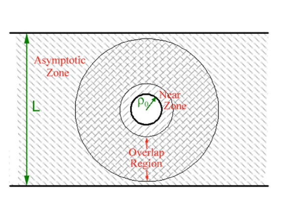
Figure 4: The division of the spacetime into two overlapping zones: the near zone $\rho\gtrsim\rho_{0}$ where the perturbative parameter is $L^{-1}$, the asymptotic zone $\rho_{0}\ll\rho\sim L$ where the perturbative parameter is $\rho_{0}$ and the overlap region in between.

The near zone:

for $\rho\gtrsim\rho_{0}$ we expand the solution around the $d$-dimensional Schwarzschild solution characterized by $\rho_{0}$ (see section 3). Since $\rho\sim\rho_{0}$ in this zone, the small dimensionful parameter of the expansion in this zone would be $L^{-1}$. Notice that when $L\rightarrow\infty$ (i.e., the limit of “unfolding” the compact dimension) we are left only with the first term (zeroth order) of the expansion which is the $d$-dimensional Schwarzschild solution. The next terms represent the influence of the compact dimension on the black hole’s metric. From the point of view of the near zone, as the period $L$ is large compared to $\rho_{0}$, the terms in the expansion series become smaller and the convergence of the perturbation series is better.

The asymptotic zone:

for $\rho_{0}\ll\rho\sim L$ we expand around the flat background with a compact dimension of size $L$. Here we take $\rho_{0}$ the size of the black hole as the small dimensionful parameter (this is the so called post-newtonian expansion, see section 2, with the matching added as a boundary condition). The terms in the expansion represent the distortion of the flat spacetime (with a compact dimension) due to the presence of the black hole and its “mirror images”. From the point of view of the asymptotic zone, as the mass of the black hole becomes smaller, the terms in the expansion series become smaller and the convergence of the perturbation series is better.

The overlap region:

each one of the expansions cannot be determined independently since it requires boundary conditions at the overlap. Hence, it carries free parameters that should be determined by matching to the other expansion in the overlap region $\rho_{0}\ll\rho\ll L$. This is achieved by comparing the multipoles of the expansions order by order; In the asymptotic zone we look at the multipoles in the limit $\rho\ll L$ and match them with the multipoles of the near zone expansion in the limit $\rho\gg\rho_{0}$.

There are three parameters that determine the matching procedure for each term in the multipole expansion:

• The order of the multipole expansion which we denote by $n$. A term of order $n$ in the asymptotic zone expansion is proportional to $\rho_{0}^{n}$ while a term of the same order in the near zone is proportional to $({1}/{L})^{n}$.

• The multipole number $l$. In each order a given multipole can have contributions from lower multipoles (via non-linear sources from the same zone, e.g. addition of angular momenta) and from matching which is linear and as such can be performed only between identical multipoles in both zones.

• The number of dimensions $d$.

The interplay between these three parameters $l,n,d$ creates the matching pattern which we describe below.

In the previous sections we obtained the linear perturbations around the exact solutions (equations (75) and (11)). In order to get non-linear corrections by the method of successive approximations we substitute in Einstein’s equations expansions of the form

$$g_{\mu\nu}=g^{(0)}_{\mu\nu}+g^{(1)}_{\mu\nu}+g^{(2)}_{\mu\nu}+\cdots+g^{(n)}_{\mu\nu}+\cdots\,,$$ (87)

where $g^{(0)}_{\mu\nu}$ is the exact solution. For each term of this expansion we get an equation for the metric components of the form

$$\mathcal{L}(g^{(n)}_{\mu\nu})=\mathcal{F}_{n}(g^{(n-1)},g^{(n-2)},\ldots,g^{(1)})\,,$$ (88)

where the superscript $n$ denotes the order in the perturbation, $\mathcal{L}$ is linearized operator (which is second order and independent of $n$) and $\mathcal{F}_{n}$ stands for nonlinear terms that are functions of the previous orders and their derivatives. Since the asymptotic zone expansion is in the harmonic gauge, $\mathcal{L}$ there is simply the laplacian. In the near zone, as we saw in section 3, the operator is more involved and it is given by $\mathcal{L}^{l}_{\rm Heun}$, defined in (77). At each order one is free to add to the metric a solution to the homogeneous equation (an element of $\mbox{ker}(\mathcal{L})$). The homogeneous solution of any order $n$ can be expanded into multipoles. Thus we can write the general form of the $n$-th correction to the metric in the form

$$g_{\mu\nu}^{(n)}=g_{\mu\nu,(p)}^{(n)}+\sum_{l=0}^{\infty}c^{(n)}_{l}\,f^{(n)\,l}_{\mu\nu}(\rho)\,\Pi_{0}^{l,d}(\chi)\,.$$ (89)

The first term is the particular solution of order $n$. The second term is the multipole expansion of the homogeneous solution where $\Pi_{0}^{l,d}(\chi)$ is the spherical harmonics function, defined in (16) (remember that we have $\mathop{\rm SO}\nolimits(d-2)$ symmetry). $f^{(n)\,l}_{\mu\nu}(\rho)$ is the multipole radial function and $c^{(n)}_{l}$ are coefficients that we should determine using the matching procedure for each multipole $l$ and order $n$ (in $d$ dimensions). For the matching we would have to expand the particular solutions to multipoles as well.

¿From the previous subsection we learn that in the limit $\rho\gg\rho_{0}$ the Schwarzschild and harmonic coordinates coincide. Hence we are allowed to compare leading terms in the two zones without coordinate transformations. Moreover, in this limit ($\rho\gg\rho_{0}$) the homogeneous linear operator in the near zone becomes the laplacian (Einstein’s equations in this limit coincides with the newtonian poisson equations). Therefore, in both zones, the leading terms will be multipole functions of the laplacian, namely, leading terms that their dependence on $\rho$ goes like $\rho^{l}$ or $\rho^{-(l+d-3)}$ (see (19)).

In the homogeneous solutions of the near zone the leading terms (the ones to be matched) behave like $\rho^{l}$ (when one takes the limit $\rho\gg\rho_{0}$). The component with the subleading behavior $\rho^{-(l+d-3)}$ is determined by the boundary condition of regularity at the horizon. This can be seen explicitly from the solution that we have for $E_{l}$ in section 3.3.3. The Riemann P-Symbol (appendix A) shows us that the asymptotic behavior of the two power series expansions at infinity is $\rho^{l}$ or $\rho^{-(l+d-3)}$. For the asymptotic zone the role is reversed – the leading term in the overlap zone ($\rho\ll L$) is $\rho^{-(l+d-3)}$ while the subleading term $\rho^{l}$ is fixed by the boundary conditions at infinity.

We summarize the discussion above using a graphic representation of the multipole expansion for multipole number $l$ in figure 5. The numbers stand for the order in the multipole expansion. The two rows of cells represent the expansion in the asymptotic zone (above) and in the near zone (below). The left side of each cell contains the leading term in the overlap region (that should “receive” the information from the matching). The right side of each cell contains the appropriate term to match the left side of different cell. The horizontal part in the cell reminds us the order of perturbation — $\rho_{0}^{n}$ in the asymptotic zone and $L^{-n}$ in the near zone. The matching procedure actually becomes a process of determining which cell’s left side receives information from which cell’s right side (as we will see, not all the cells are relevant for this process).

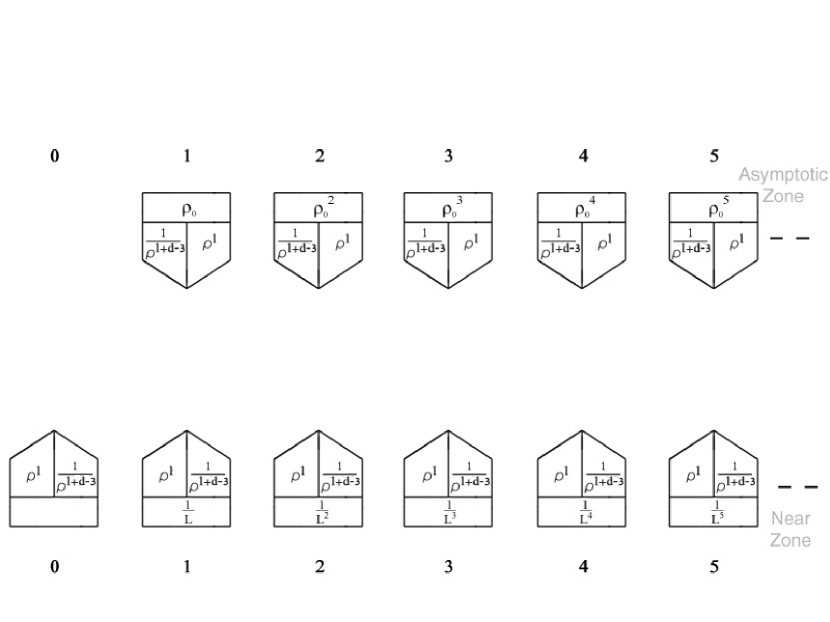
Figure 5: The representation of the expansion in the near and asymptotic zones for a multipole moment $l$, before the matching. Each cell in the upper row stands for a term in the asymptotic zone expansion and each cell in the lower row stands for a term in the near zone expansion. Each cell consists of the small parameter in the appropriate power and two terms to be matched.

To determine the pattern of perturbation, namely the basic “dialogue arrows” of information flow in a diagram such as figure 5, the basic observation comes from dimensional analysis. A mass multipole moment of multipole number $l$, $\mathcal{M}_{l}$, is defined as

$$\mathcal{M}^{0}_{l_{~{}i_{1},\dots,i_{n}}}\sim\int\!dm\,x_{i_{1}}x_{i_{2}}\ldots{x_{i_{l}}}\,,$$

where the indices $i_{j}$ denote the cartesian coordinates, and the superscript $0$ is a reminder that these are multipoles at the origin. The gravitational field of multipole of order $l$ of mass distribution at the origin behaves like

$$\frac{\mathcal{M}^{0}_{l}}{\rho^{l+d-3}}\,,$$

and the multipole moment itself has the length dimensions

$$\left[\mathcal{M}^{0}_{l}\right]=l+d-3\,.$$ (90)

Such mass multipoles at the origin are used to supply matching boundary conditions for the asymptotic zone. Suppose we are at order $n$ in the asymptotic zone so that

$$\mathcal{M}^{0}_{l}\sim{\rho_{0}^{~{}n}\over L^{m}}\,,$$ (91)

where $m$ is the near zone order from which it was matched. Comparing (90) and (91) we conclude that

$$n-m=\left[\mathcal{M}^{0}_{l}\right]=l+d-3\,,$$ (92)

namely, upward pointing “dialogue arrows” have a step-size of $l+d-3$. In a similar manner the multipole moments at infinity (used to supply boundary conditions for the near zone) yield

$$n-m=\left[\mathcal{M}^{\infty}_{l}\right]=-l\,,$$

since the (dimensionless) gravitational field behaves like

$$\mathcal{M}^{\infty}_{l}\rho^{l}\,.$$

Namely, downward pointing “dialogue arrows” have a step-size of $+l$.

Alternatively, the same result can be described from the following point of view. In the perturbation process we expand a dimensionless quantity which satisfied Laplace’s equation in the two zones and compare the expansions in the overlap zone. In the matching process we identify two terms that make one dimensionless quantity in the overlap region. The process is demonstrated in figure 6. Looking at a cell of order $m$ in the near zone, we see that the corresponding term in the expansion is proportional to $\frac{1}{L^{m}\,\rho^{l+d-3}}$. In order to create a dimensionless quantity, we have to match this term to order $n=l+m+d-3$ in the asymptotic zone. Then we have a leading term proportional to

$$\frac{\rho_{0}^{l+m+d-3}}{L^{m}\,\rho^{l+d-3}}\,,$$

up to a numerical constant. Using the same argument, this cell in the asymptotic zone is matched to the cell $m^{\prime}=n+l=m+2l+d-3$ in order to create the dimensionless quantity

$$\frac{\rho_{0}^{n}\,\rho^{l}}{L^{n+l}}\,.$$

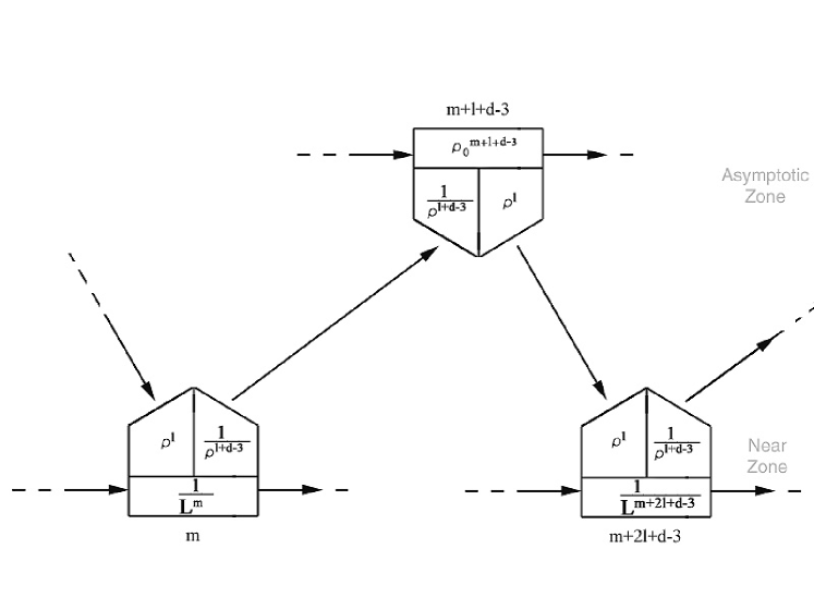
Figure 6: Two steps in the matching procedure. A term of order $m$ and multipole number $l$ in the near zone determines the multipole of order $n=m+l+d-3$ in the asymptotic zone. Afterwards the latter is used to determine a term of order $m^{\prime}=n+l=m+2l+d-3$ in the near zone.

Apparently, this process can continue to create an infinite chain of matchings for each multipole which consists of two unequal steps; from the near to asymptotic zone we have a step of $\Delta n=l+d-3$ orders and from the asymptotic to the near we have a step of $\Delta n=l$ orders.

4.3 Pattern of the dialogue

Let us look in detail into the pattern of the dialogue. We would like to summarize all the “information flow arrows” between the various orders and to conclude how the computation should be performed to determine the metric up to a prescribed order in one of the zones (following what we term “the critical route”).

First we note that since our problem is defined with reflection symmetry $z\rightarrow-z$, one should consider only multipoles that satisfy this symmetry. Applying the transformation $\chi\rightarrow\chi+\pi$ in (17) shows that only even multipoles are relevant for our expansions.

We summarize the information flow arrows for a diagram such as figure 5:

• Within a zone.

  These are the ordinary non-linear sources of the perturbation procedure. At order $n$ there can be a non-zero source only if there are some non-zero metrics at orders $n_{i}<n$ such that some linear combination of $n_{i}$ with integer positive coefficients yields $n$.

• Inter-zone arrows.

  We saw above that arrows going “down” (from the asymptotic to the near zone) advance by $l$ orders, while those going in the reverse direction advance by $l+d-3$ orders. Since $l$ can only be even there are two basic steps: $2$ and $d-3$.

Finally there is an “initial condition”: the leading correction to the zeroth order metrics is the newtonian potential at order $d-3$ in the asymptotic zone. Therefore the larger $d$ is there will be more orders where the metric vanishes.

¿From a practical point of view it is especially important to determine the “critical route”. Namely, suppose we wish to compute the metric up to a prescribed order $n$ in a certain zone. Which orders must be determined on the way? Clearly we should know all the lower orders in that zone. In addition we should have information from the other zone. If the original zone in which we were interested is the near zone we should know the metric at the asymptotic zone at orders $n-l$ for all even $l$, and similarly if it were the asymptotic one we need to know all the $n-(d-3)-l$ orders of the near zone. We see that in both cases the limiting $l$ is the monopole $l=0$ which sets the critical route to arrive from the other zone: to reach the near (asymptotic) order $n$ the critical route passes through the asymptotic (near) order $n$ ($n-d+3$). It is clear that the procedure does not run into closed loops since the sum of the two step-sizes, being $d-3$, is greater than 0, and in that sense there are sufficient boundary conditions to determine the expansion, namely it is well-posed.

In order to make this analysis more concrete we shall first outline the first steps in the procedure for $d=5$ which is somewhat special and then do the same for some general $d>5$.

In the case of 5 dimensions $d-3=2$ and this implies that only the even orders are involved in the expansion (the same holds true for any odd dimension). Hence in 5 dimensions we actually expand in the small parameters $\rho_{0}^{2}$ and $\frac{1}{L^{2}}$ (see figure 7). This is a great simplification to the perturbation scheme. Moreover, all the even multipole functions (see (82)) are polynomials in 5 dimensions.

In figure 7 we show the first steps in the matching procedure in 5 dimensions, until the fourth order. In order to have the metric until the fourth order in the two zones we need, besides the particular solutions, to match the monopole ($l=0$) and the quadrupole ($l=2$). In order to obtain higher orders we will have to add higher multipoles to the matching. Note that we have to know the fourth order in the asymptotic zone in order to get the fourth order in the near zone. This situation is rather different for $d>5$.

Figure 7: The first steps in the matching procedure in 5 dimensions. Until the fourth order only monopole and quadrupole matches appear in the two zones. Each one of the matches is represented by a different color. The newtonian approximation enters in the second order in the asymptotic zone. It is clear from the figure that the monopole is the limiting and hence the most “fresh” multipole that should be determined for a certain order.

In 5d it is easy to understand that the method is well-posed. If we look at a cell of order $n$ in the near zone, then all the (even) multipoles from $l=0$ to $l=n$ are determined from the previous orders in the asymptotic zone when the monopole is the last to be matched — it is determined from the same order but in the asymptotic zone. We do not have to determine any multipole higher than $n$ because they do not appear at this order — in order to create a dimensionless quantity out of $\rho^{n+k}$ for $k\geq 1$ we have to multiply it at least by $\frac{1}{L^{n+k}}$ (thus this multipole will appear at order $n+k$ at least in the near zone). Therefore, for any order until $n$ the metric in the near zone is determined. Similar argument is valid for the asymptotic zone as well. let us look at a cell of order $n$ in the asymptotic zone. All the multipoles from $l=0$ to $l=n-2$ are determined by matching to the near zone when $l=0$ (the monopole) is the last one to be matched (it is matched with the cell of $2$ orders before) — see figure 7. Therefore, the information for any cell comes from the cells of lower orders in the other zone in 5d.

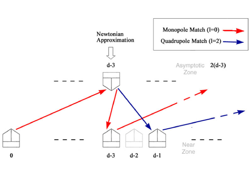
Figure 8: The first steps in the matching procedure for $d>5$. Compare with the previous figure (the same in 5 dimensions). Here the first quadrupole matching in the near zone is done before the second correction to the monopole.

The first steps in the matching for $d>5$ dimensions are shown in figure 8. Since the newtonian approximation enters at the order $d-3>2$, the post-newtonian correction comes at $2\,(d-3)$. The first quadrupole contribution in the near zone comes in $(d-3)+2=d-1$. Then, as opposed to the case of $d=5$, the second matching of the monopole in the near zone comes after the quadrupole matching, since $2\,(d-3)>d-1$. As we go to higher dimensions, there are more multipoles in the near zone that we can match with the multipoles in the newtonian approximation before adding the second correction to the monopole. This can be calculated precisely: The length of a step of a match from the asymptotic zone to the near zone is $\Delta n=l$. The distance between the newtonian and post-newtonian approximations is $\Delta n=d-3$. So any multipole that satisfy $l<d-3$ comes before the second correction to the monopole. An interesting limit is when $d\rightarrow\infty$. Then, the newtonian approximation is enough to determine all the orders of expansion in the near zone.

5 Matching results

After describing the procedure in general, let us start and calculate the first coefficients of the approximate solution. Note that in the matching process it is enough to match a single metric component to guarantee the matching of the whole metric. For our purposes it will be convenient to consider for the matching the dimensionless quantity ${g_{\chi\chi}}/{\rho^{2}}$.

5.1 The first monopole match

Actually there is a zeroth monopole match which relates the mass measured asymptotically (through the newtonian potential) with the $\rho_{0}$ parameter of the Schwarzschild solution, namely a matching between the zeroth order in the near zone and order $n=d-3$ in the asymptotic zone (the first red arrow in figures 7 and 8). This match was done in section 2 (based on [39]) and gives the identification $\rho_{0}^{d-3}=\frac{16\,\pi\,G_{d}\,M}{(d-2)\,\Omega_{d-2}}$.

The first monopole match is between the monopole in the newtonian approximation ($n=d-3$) and the first monopole correction to the $d$-dimensional Schwarzschild solution. Being the $l=0$ correction the spherical symmetry of the black hole will not be lost, but rather the physical interpretation is that the black hole is placed in a region with a constant non-zero gravitational potential due to the array of image black holes.

First we expand the newtonian approximation in multipoles around the origin including not only the monopole term but also the quadruple in anticipation of the computation of eccentricity. The expansion around $\rho=0$ in polar coordinates $(\rho,\chi)$ is

$$\frac{g_{\chi\chi}^{\mbox{(asymp)},d-3}}{\rho^{2}} = \frac{\rho_{0}^{d-3}}{d-3}\sum_{n=-\infty}^{\infty}\frac{1}{(r^{2}+(z-nL)^{2})^{\frac{d-3}{2}}}$$ (93)

$$= \frac{1}{d-3}\cdot\frac{\rho_{0}^{d-3}}{\rho^{d-3}}+\frac{2}{d-3}\cdot\frac{\rho_{0}^{d-3}}{L^{d-3}}\,\zeta(d-3)+$$

$$+\frac{(d-2)\,\rho^{2}\,\rho_{0}^{d-3}}{4\,L^{d-1}}\,\zeta(d-1)\,\Pi^{2,d}_{0}(\chi)+\mathcal{O}(\rho^{4})\,,$$

where $\zeta$ is Riemann’s zeta function and

$$\Pi^{2,d}_{0}(\chi)=\frac{1}{d-2}\,\left(\cos^{2}(\chi)\,(d-1)-1\right),$$

according to the Rodrigues formula (17). The superscript “$\mbox{(asymp)},d-3$” indicates that this is the correction of order $d-3$ in the asymptotic zone. In the same way we will denote the expansions in the near zone by the superscript “(near)”. Note that there is no dipole term in the expansion (or any odd multipole) due to the symmetry $\chi\rightarrow\chi+\pi$.

Recall the expressions that we had for the metric monopole perturbations (71)–(73). Comparison with the monopole term in (93) gives us the value of the matching constant $C_{1}$ for the first correction to the metric in the near zone ($n=d-3$)

$$C_{1}=\zeta(d-3)\,\frac{\rho_{0}^{d-3}}{L^{d-3}}\,.$$

The final form of the metric in the near zone with the first monopole correction is

$$\framebox{$\begin{array}[]{rcl}~{}\rule[-5.69054pt]{0.0pt}{22.76219pt}g_{\chi\chi,d}^{\mbox{near}}&=&\displaystyle\rho^{2}\left(1+\frac{2\,\zeta(d-3)\,\rho_{0}^{d-3}}{(d-3)\,L^{d-3}}\right)+\mathcal{O}\left(\frac{1}{L^{d-2}}\right),\\ ~{}\rule[-5.69054pt]{0.0pt}{22.76219pt}g_{tt,d}^{\mbox{near}}&=&\displaystyle-\left(1-\frac{\rho_{0}^{d-3}}{\rho^{d-3}}\right)\left(1-\frac{2\,\zeta(d-3)\,\rho_{0}^{d-3}}{L^{d-3}}\right)+\mathcal{O}\left(\frac{1}{L^{d-2}}\right),\\ ~{}\rule[-5.69054pt]{0.0pt}{22.76219pt}g_{\rho\rho,d}^{\mbox{near}}&=&\displaystyle\left(1-\frac{\rho_{0}^{d-3}}{\rho^{d-3}}\right)^{-1}\left(1+\frac{2\,\zeta(d-3)\,\rho_{0}^{d-3}}{(d-3)\,L^{d-3}}\right)+\mathcal{O}\left(\frac{1}{L^{d-2}}\right).\end{array}$}$$ (94)

As mentioned above this monopole correction can be attributed to the non-zero newtonian potential at infinity of the near zone. The same result can be obtained in a less formal way by rescaling of $t$ reflecting in this way the change in the asymptotic boundary conditions.

Since there is no change in the shape of the black hole we can measure the effect of the correction by calculating the correction to the dimensionless quantity $\kappa^{d-2}\,A_{d-2}$ where $\kappa$ is the surface gravity of the horizon and $A_{d-2}$ is its $(d-2)$-dimensional area.

To find the area we note that the horizon in this approximation is located at a constant $\rho_{H}$ which is defined as the root of $g_{tt}(\rho)$=0. Using the approximated metric above we get that the horizon does not move (in our gauge)

$$\rho_{H}^{d-3}=\rho_{0}^{d-3}+\mathcal{O}\left(\frac{1}{L^{d-1}}\right).$$

The area of the horizon is

$$A_{d-2} = g_{\chi\chi}(\rho_{H})^{\frac{d-2}{2}}~{}\Omega_{d-2}$$ (95)

$$= \rho_{0}^{d-2}\,\Omega_{d-2}\left(1+\frac{(d-2)\,\zeta(d-3)\,\rho_{0}^{d-3}}{(d-3)\,L^{d-3}}+\mathcal{O}\left(\frac{1}{L^{d-1}}\right)\right).$$ (96)

The surface gravity calculated using (129) of appendix B is

$$\kappa=\left.\frac{1}{2}\,\frac{\mid\!\partial_{\rho}g_{tt}(\rho)\!\mid}{\sqrt{-g_{\rho\rho}(\rho)\,{g_{tt}(\rho)}}}\,\right|_{\rho=\rho_{H}}.$$

Substituting the approximate metric we get

$$\kappa=\frac{d-3}{2\rho_{0}}\,\left(1-\frac{(d-2)\,\zeta(d-3)}{d-3}\cdot\frac{\rho_{0}^{d-3}}{L^{d-3}}\right)+\mathcal{O}\left(\frac{1}{L^{d-1}}\right).$$

Combining the results together we obtain

$$\framebox{$~{}\rule[-5.69054pt]{0.0pt}{22.76219pt}\displaystyle\kappa^{d-2}\,A_{d-2}=\left(\frac{d-3}{2}\right)^{d-2}\,\Omega_{d-2}\,\left(1-(d-2)\,\zeta(d-3)\cdot\frac{\rho_{0}^{d-3}}{L^{d-3}}\right)+\mathcal{O}\left(\frac{\rho_{0}^{d-1}}{L^{d-1}}\right).$}$$ (97)

5.2 Matching multipoles to the newtonian approximation

Our next goal is to obtain an expression for the deviation from spherical symmetry — the eccentricity of the horizon. For this purpose we have to match the quadrupole term in the near zone to the newtonian approximation. In this subsection we give a more general recipe, matching any multipole to the newtonian approximation.

As was explained in the previous section, this matching is important for higher multipoles as we increase the number of dimensions. From the matching scheme we learn that the multipoles in the newtonian approximation match with $\Delta n=l$ orders higher in the near zone expansion.

Let us count the number of constants to match. Given $l$ there are two radial solutions in the near zone. Regularity at the horizon fixes a particular combination and so it remains to set the normalization of this combination by comparing the leading terms from both zones. Thus we need to determine a single constant per multipole.

In the near zone we have the multipole functions written in terms of solutions of a Hypergeometric equation (recall (76) and (81)). Regularity of the metric at the horizon requires that the relevant solution of the Hypergeometric equation be regular there. The horizon is located at $X=1$ when we use the variable $X$ as we defined in (74)

$$X=\left(\frac{\rho}{\rho_{0}}\right)^{d-3}.$$

Using the Riemann P-Symbol of (76) we can obtain the regular solution at $X=1$ (see [45]) and substitute it into (81)

$$E_{l}=\left(1-(d-3)\,X\,\frac{d}{dX}\right)\left(1-X)\,_{2}\!F_{1}(1-\frac{l}{d-3},2+\frac{l}{d-3},2\,;1-X\right).$$ (98)

The correction to the near zone metric of order $l+d-3$ is proportional to $E_{l}$

$$\frac{g_{\chi\chi}^{\mbox{(near)},l+d-3}}{\rho^{2}}=D_{l}\,\rho_{0}^{l}\,E_{l}(X)\,\Pi^{l,d}_{0}(\chi)\,,$$ (99)

where $D_{l}$ is the matching constant which depends on the multipole and the dimension. This constant will be determined by matching to the asymptotic zone. If $d-3>l$ the newtonian approximation suffices and otherwise non-linear terms from lower orders should be added.

In order to match this solution in the overlap zone we have to find its leading term as $X\to\infty$. The regular solution of the Hypergeometric equation (76) at $X=1$ can be written as a combination of the two solutions at infinity, using the identity (see [45])

$${}_{2}\!F_{1}(\alpha,\beta,\gamma;1-X) = c_{1}\,(X-1)^{-\alpha}\,_{2}\!F_{1}\left(\alpha,\alpha-\gamma+1,\alpha-\beta+1;\frac{1}{1-X}\right)+$$ (100)

$$+c_{2}\,(X-1)^{-\beta}_{2}\!F_{1}\left(\beta,\beta-\gamma+1,\beta-\alpha+1;\frac{1}{1-X}\right),$$

where

$$c_{1} = \frac{\Gamma(\gamma)\,\Gamma(\beta-\alpha)}{\Gamma(\gamma-\alpha)\,\Gamma(\beta)}\,,$$

$$c_{2} = \frac{\Gamma(\gamma)\,\Gamma(\alpha-\beta)}{\Gamma(\gamma-\beta)\,\Gamma(\alpha)}\,.$$

Hence, in our case the leading term of the Hypergeometric function is

$$c_{1}X^{-\alpha}=\frac{\Gamma(2)\,\Gamma(\frac{2\,l}{d-3}+1)}{\Gamma(1+\frac{l}{d-3})\,\Gamma(2+\frac{l}{d-3})}\,X^{\frac{l}{d-3}-1}\,.$$

Substituting into (98) we obtain the leading term in $E_{l}$ as $X\to\infty$

$$E_{l}\sim\frac{\Gamma(\frac{2\,l}{d-3}+1)}{\Gamma(1+\frac{l}{d-3})\,\Gamma(2+\frac{l}{d-3})}\,(l-1)\left(\frac{\rho}{\rho_{0}}\right)^{l}.$$ (101)

Note that the exponent $\sim\rho^{l}$ of the leading term is exactly what we anticipate for multipole function of order $l$. The determination of the prefactor allows one to obtain the constants $D_{l}$ by matching with the asymptotic zone.

5.3 The eccentricity

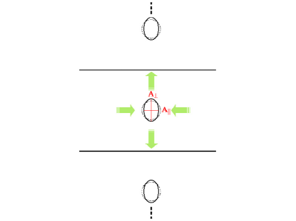
Figure 9: The effective “mirror” images induce tidal forces that stretch the horizon of the black hole. We quantify this by the eccentricity which is defined using two sections of the horizon.

The lowest order deviation from spherical symmetry of the near zone metric occurs in $n=(d-3)+2=d-1$, where we match the quadrupole (see figures 7 and 8). We can quantify deviation of the black-hole from spherical symmetry by the eccentricity of the horizon. We define the eccentricity of the horizon as in [20]

$$\epsilon\equiv\frac{A_{\perp}}{A_{\parallel}}-1\,,$$ (102)

where $A_{\parallel}$ is the $(d-3)$-dimensional area of the equatorial sphere at $\chi=\frac{\pi}{2}$ and $A_{\perp}$ is the $(d-3)$-dimensional area of the polar sphere at $\chi=0,\pi$ (see figure 9) . Since $g_{\chi\chi}$ is a function only of $\rho$ and $\chi$ (recall the symmetry $\mathop{\rm SO}\nolimits(d-3)$) we obtain

$$A_{\parallel} = \Omega_{d-3}\,g_{\chi\chi}^{\frac{d-3}{2}}\left(\rho=\rho_{H},\chi=\frac{\pi}{2}\right),$$

$$A_{\perp} = \Omega_{d-4}\int_{0}^{\pi}g_{\chi\chi}^{\frac{d-3}{2}}(\rho=\rho_{H})\sin^{d-4}(\chi)d\chi\,.$$

Matching the quadrupole in the near zone in order $n=d-1$ to the newtonian approximation $n=d-3$ (equating the quadrupole terms — $l=2$ — in (99) and (93) using the leading term (101) of the quadrupole radial function in the near zone) we obtain

$$\framebox{$~{}\rule[-5.69054pt]{0.0pt}{22.76219pt}\displaystyle D_{2}=\frac{(d-2)\,\zeta(d-1)\,\Gamma(1+\frac{2}{d-3})\,\Gamma(2+\frac{2}{d-3})}{\Gamma(\frac{4}{d-3}+1)}\cdot\frac{\rho_{0}^{d-1}}{L^{d-1}}\,.$}$$ (103)

Therefore

$$\frac{g_{\chi\chi}^{\mbox{(near)},d-1}}{\rho^{2}}=D_{2}\,E_{2}(X)\,\Pi_{0}^{2,d}(\chi)\,.$$ (104)

For the calculation of the eccentricity we need the value of $E_{2}(X)$ at the horizon, namely, $X=1$. From (98) we can see that

$$E_{2}(X=1)=d-3\,.$$ (105)

As the first non-spherical term is at order $n=d-1$ in the near zone, the leading term in the eccentricity is proportional to $\frac{\rho_{0}^{d-1}}{L^{d-1}}$. Thus, we have to substitute $g_{\chi\chi}^{\mbox{(near)},d-1}$ in the expression for the eccentricity (102) and find the coefficient of $\frac{\rho_{0}^{d-1}}{L^{d-1}}$ in the expansion. First we expand

$$\left.g_{\chi\chi}^{\frac{d-3}{2}}\,\right|_{\rho=\rho_{H}} = \rho_{0}^{d-3}\,\left(1+\cdots+\rho_{0}^{2}\,D_{2}\,(d-3)\,\Pi^{2,d}_{0}(\chi)+\mathcal{O}\left(\frac{1}{L^{d}}\right)\right)^{\frac{d-3}{2}}$$ (106)

$$= \rho_{0}^{d-3}\,\left(1+\cdots+\frac{(d-3)^{2}}{2}\,\rho_{0}^{2}\,D_{2}\,\Pi^{2,d}_{0}(\chi)+\mathcal{O}\left(\frac{1}{L^{d}}\right)\right),$$

and at $\chi={\pi}/{2}$ we get

$$\left.g_{\chi\chi}^{\frac{d-3}{2}}\,\right|_{\rho=\rho_{H},\chi=\frac{\pi}{2}}=\rho_{0}^{d-3}\,\left(1+\cdots-\frac{(d-3)^{2}}{2\,(d-2)}\,\rho_{0}^{2}\,D_{2}+\mathcal{O}\left(\frac{1}{L^{d}}\right)\right),$$ (107)

where the ellipsis stand for monopole corrections which, of course, do not contribute to the eccentricity. Substituting in (102) we obtain

$$\epsilon=\frac{(d-3)^{2}}{2}\,\rho_{0}^{2}\,D_{2}\,\left(\frac{\Omega_{d-4}}{\Omega_{d-3}}\int_{0}^{\pi}\Pi^{2,d}_{0}(\chi)\,\sin^{d-4}(\chi)\,d\chi+\frac{1}{d-2}\right)+\mathcal{O}\left(\frac{\rho_{0}^{d}}{L^{d}}\right).$$ (108)

The integral gives us

$$\int_{0}^{\pi}\Pi^{2,d}_{0}(\chi)\,\sin^{d-4}(\chi)\,d\chi=\frac{1}{d-2}\,\Gamma\left(\frac{d-3}{2}\right)\,\left(\frac{2^{d-2}(d-1)\,\Gamma(\frac{d+1}{2})}{\Gamma(d-1)}-\frac{d\,\sqrt{\pi}}{\Gamma(\frac{d}{2}-1)}\right).$$ (109)

This using identities of the Gamma function (see [45]) yields the final formula for the eccentricity

$$\framebox{$~{}\rule[-5.69054pt]{0.0pt}{22.76219pt}\displaystyle\epsilon=\frac{(d-3)^{4}\,(\Gamma(2+\frac{2}{d-3}))^{2}\,\zeta(d-1)}{8\,(d-2)\,\Gamma(\frac{4}{d-3})}\cdot\frac{\rho_{0}^{d-1}}{L^{d-1}}+\mathcal{O}(\frac{\rho_{0}^{d}}{L^{d}})\,.$}$$ (110)

We can also write the eccentricity as a function of a differently normalized variable: the relative size of the horizon in conformal coordinates which we define as (see [20])

$$\eta\equiv{2\,\rho_{h}\over L}={2^{d-5\over d-3}\,\rho_{0}\over L}\,,$$ (111)

where $\rho_{h}$ is the location of the horizon in conformal coordinates $ds^{2}=e^{2\,\hat{A}}\,dt^{2}+e^{2\,\hat{B}}\,(dr^{2}+dz^{2})+e^{2\,\hat{C}}\,d\Omega_{d-3}^{~{}2}$ which were used extensively in the literature and will be used here only for setting the normalization of $\eta$. $\eta$ is the same quantity denoted by $x$ in [20, 21]. One gets

$$\epsilon = \frac{(d-3)^{4}\,(\Gamma(2+\frac{2}{d-3}))^{2}\,\zeta(d-1)}{(d-2)\,\Gamma(\frac{4}{d-3})}\cdot 2^{-\frac{(d-4)\,(d+1)}{d-3}}\cdot\eta^{d-1}+\mathcal{O}(\eta^{d})$$ (112)

$$\equiv \epsilon_{1}\,\eta^{d-1}\,.$$

The constants $\epsilon_{1}(d)$ are illustrated in figure 10 and in the next table.

d $$\epsilon_{1}$$

5

6

7

8

9

10

Figure 10: A plot of the function $\epsilon_{1}(d)$ which gives the $d$-dependence of the first coefficient of proportionality in the expansion of the eccentricity, normalized as in (5.20). Note that $\epsilon_{1}(d)$ is monotonously decreasing to 0.

5.4 The “Archimedes” effect

We define the inter-polar distance $L_{\rm poles}$ to be the proper distance between the “poles” of the black hole measured around the compact dimension

$$L_{\rm poles}=2\,\int_{z_{H}}^{L/2}dz\,\sqrt{g_{zz}}\,,$$ (113)

where $z_{H}$ denotes the location of the horizon. It is convenient to define a dimensionless parameter out of $L_{\rm poles}$

$$y\equiv 1-{L_{\rm poles}\over L}\,.$$ (114)

Thus $y$ is the relative decrease in the size of the compact dimension at $r=0$ due to the presence of the black hole. Like any other property of the system it is a function of the single dimensionless quantity which characterizes it, which we choose to be $\eta$, the relative size of the horizon in conformal coordinates defined in (111).

$y(\eta)$ is an interesting quantity to compute in our framework since it involves both zones in an essential way. The way to compute it is to pick some mid-point $Z$, divide the integration between the two zones

$$\frac{1}{2}\,L_{\rm poles}=\int_{z_{H}}^{Z}dz\,\sqrt{g_{zz}^{\mbox{(near)}}}+\int_{Z}^{L/2}dz\,\sqrt{g_{zz}^{\mbox{(asymp)}}}\,,$$ (115)

and confirm that the result is independent of the choice of mid-point (up to the specified order in $\eta$).

Clearly $y(\eta=0)=0$. Here we wish to compute $y$ to first order in $\eta$. Which order is required on each zone for the evaluation? Near the horizon it is enough to take the zeroth order, that is the Schwarzschild solution with no corrections (a factor of $\eta$ multiplies it as all distances scale with $\rho_{0}$ and the definition of $y$ includes a division by $L$). In the asymptotic zone one would need in principle the first order correction (in $\eta$), but since the leading order newtonian potential is of order $\eta^{d-3}$ and $d\geq 5$ it suffices to consider again the zeroth order, namely flat compactified space.

Having the matching with the asymptotic zone in mind we write the Schwarzschild metric in the following conformal coordinates

$${1\over\rho_{h}^{~{}2}}\,ds^{2~{}\mbox{(near)}}=-\left({1-\psi\over 1+\psi}\right)^{2}\,dt^{2}+(1+\psi)^{4\over d-3}\,\left(d\rho^{2}+\rho^{2}\,d\Omega^{2}_{d-2}\right),$$ (116)

where

$$\psi=\left(\rho_{h}\over\rho\right)^{d-3}.$$ (117)

These coordinates approach the newtonian gauge as $\rho\gg\rho_{h}$.

We may now compute the contribution from the near zone to (115)

$${1\over L}\,\int_{z_{H}}^{Z}dz\,\sqrt{g_{zz}^{\mbox{(near)}}}=$$ (118)

transforming to a dimensionless $\zeta\equiv z/\rho_{h}$

$$={\rho_{h}\over L}\,\int_{1}^{Z/\rho_{h}}\left(1+{1\over\zeta^{d-3}}\right)^{2\over d-3}\,d\zeta=$$ (119)

adding $(+1-1)$ to the integrand in order to separate the part which diverges with $Z$

$$={\rho_{h}\over L}\,\left[\left({Z\over\rho_{h}}-1\right)+\int_{1}^{Z/\rho_{h}}\left(\left(1+{1\over\zeta^{d-3}}\right)^{2\over d-3}-1\right)d\zeta\right]=$$ (120)

transforming to $w\equiv 1/\zeta$ in order to facilitate taking the limit $\rho_{h}\sim\eta\to 0$

$$= {Z\over L}+{\rho_{h}\over L}\,\left[\int_{\rho_{h}/Z}^{1}\left(\left(1+w^{d-3}\right)^{{2\over d-3}}-1\right)\,{dw\over w^{2}}-1\right]$$ (121)

$$\simeq {Z\over L}-{\rho_{h}\over L}\,I_{d}\,,$$

where the definite (and finite) integral $I_{d}$ is

$$\framebox{$~{}\rule[-5.69054pt]{0.0pt}{22.76219pt}\displaystyle I_{d}\equiv 1-\int_{0}^{1}\left(\left(1+w^{d-3}\right)^{{2\over d-3}}-1\right)\,{dw\over w^{2}}=4^{1/k}\,\sqrt{\pi}\,{\Gamma\left({k-1\over k}\right)\over\Gamma\left({1\over 2}-{1\over k}\right)}\,,\qquad k=d-3~{}$}$$ (122)

and at this order we neglect the remainder of the integral

$$-{\rho_{h}\over L}\,\int_{0}^{\rho_{h}/Z}\left(\left(1+w^{d-3}\right)^{{2\over d-3}}-1\right)\,{dw\over w^{2}}\,.$$ (123)

The contribution of the (flat metric) asymptotic zone to (115) is simply

$${1\over L}\,\int_{Z}^{L/2}dz\,\sqrt{g_{zz}^{\mbox{(asymp)}}}={1\over 2}-{Z\over L}\,,$$ (124)

where due to the low order of the calculation and the choice of coordinates we can use the same value for $Z$ in both patches, with no need for corrections arising from a further matching of the patches.

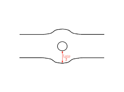
Figure 11: Illustration of the “Archimedes effect”. The small black hole repels an amount of space proportional to its size. In 5 dimensions, the black hole repels (to first order) an amount of space which is equal to its size (measured in conformal coordinates).

Summing (121), (124) according to (115) and using the definitions (114), (111) we confirm that the mid-point dependence, ($Z/L$), drops (up to the relevant order) and we get our result

$$y=2\,I_{d}\,\eta+o(\eta)\,,$$ (125)

where the function $I_{d}$ is shown in figure 12. It is monotonously increasing starting from $I_{5}=0,\,I_{6}=.6845$, tending to $1$ as $d\to\infty$. The special behavior at 5d where the “amount of space” outside the black hole remains fixed to first order in the black hole size was termed “the black hole Archimedes effect” [20] since the black hole seems to “repel” as much space as its own size (figure 11).

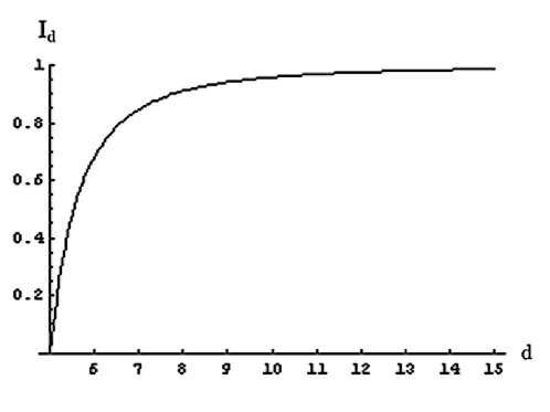
Figure 12: The function $I_{d}$ (5.30,5.33) representing the decrease in the inter-polar distance (to first order) relative to the size of the small black hole (in conformal coordinates). Note that $I_{5}=0$ and it rises monotonously to 1.

In principle we could have used the corrections to the metric computed in section 2 and subsection 5.2 to improve on this computation and determine the next to leading correction as well.

Appendix A Hypergeometric and Heun’s Equations

Let us consider a linear ordinary differential equation of second order

$$\alpha(x)\,\frac{d^{2}\,f}{dx^{2}}+\beta(x)\,\frac{df}{dx}+\gamma(x)\,f=0\,,$$ (126)

where $\alpha(x),\beta(x),\gamma(x)$ are holomorphic functions. When $\alpha(x_{0})=0$ and $\beta(x_{0})\neq 0$ (or $\gamma(x_{0})\neq 0$) then $x=x_{0}$ is a singular point of (126). This point is called regular singular point if the limits

$$\lim_{x\rightarrow x_{0}}\frac{(x-x_{0})\,\beta(x)}{\alpha(x)}=K_{1}\,,$$

and

$$\lim_{x\rightarrow x_{0}}\frac{(x-x_{0})^{2}\,\gamma(x)}{\alpha(x)}=K_{2}\,,$$

exist. The regular singular point at infinity is defined in the same way for $t=0$ in the equation

$$\frac{d^{2}\,f}{dt^{2}}+\left[\frac{2}{t}-\frac{1}{t^{2}}\,\frac{\beta(\frac{1}{t})}{\alpha(\frac{1}{t})}\right]\frac{df}{dt}+\frac{1}{t^{4}}\,\frac{\gamma(\frac{1}{t})}{\alpha(\frac{1}{t})}f=0\,,$$

which is obtained after changing the variable $x$ into $t=\frac{1}{x}$. Equation (126) is called a Fuchsian equation if all the singular points of the equation are regular.

The roots of the equation,

$$\mu^{2}+(K_{1}-1)\,\mu+K_{2}=0\,,$$

are called the characteristic exponents at $x_{0}$. There are two linearly independent solutions to the equation. Thus, at any singular regular point, there are two different expansions into power series. If the difference of the exponents is not an integer, the power series near a singular point $x_{0}$ are of the form

$$(x-x_{0})^{\mu}\sum_{i=0}^{\infty}a_{i}\,(x-x_{0})^{i}\,,$$

where $\mu$ is one of the characteristic exponents. When the difference of the exponents is an integer one of the expansions may involve a logarithmic term.

Any Fuchsian equation with 3 singular points can be transformed, by transformations of the dependent and independent variables, to a standard form where the singularities are at $0,1$ and $\infty$

$$x\,(1-x)\,\frac{d^{2}\,f}{dx^{2}}+[\gamma-(\alpha+\beta+1)\,x]\frac{df}{dx}-\alpha\,\beta\,f=0\,,$$ (127)

where $\alpha,\beta,\gamma$ are parameters. The equation in this form is called the Hypergeometric equation. The solutions of (126) can be characterized completely by the singularities and the corresponding characteristic exponents at each singularity. There exists a compact scheme to summarize the information about the solutions of the Hypergeometric equation — the Riemann P-Symbol (see for instance [45, 46])

$$P\left(\begin{array}[]{ccccccc}0&&1&&\infty&&\\ 0&&0&&\alpha&&;\ x\\ 1-\gamma&&\gamma-\alpha-\beta&&\beta&&\end{array}\right).$$

The first row of the matrix indicates the three regular singular points. The two numbers beneath each singular point are the characteristic exponents at each singular point. The expansion around $0$ of the solution with a zero exponent is the Hypergeometric function

$${}_{2}\!F_{1}(\alpha,\beta,\gamma;x)=\sum_{n=0}^{\infty}\frac{(\alpha)_{n}\,(\beta)_{n}}{(\gamma)_{n}}\,x^{n}\,,$$

where $(\alpha)_{n}\equiv\frac{\Gamma(\alpha+n)}{\Gamma(\alpha)}$ when $\alpha$ is different from a negative integer. The other 5 expansions can be obtained by transformations of this Hypergeometric function.

A Fuchsian equation with 4 singular points can be transformed similarly to a canonical form where the singularities are at $0,1,a$ and $\infty$ ($a$ can be any point in the complex plane different from the other singular points). In this canonical form the equation is called Heun’s equation [47, 48]

$$\frac{d^{2}\,f}{dx^{2}}+\left(\frac{\gamma}{x}+\frac{\delta}{x-1}+\frac{1+\alpha+\beta-\gamma-\delta}{x-a}\right)\,\frac{d\,f}{dx}+\frac{\alpha\,\beta\,x-q}{x\,(x-1)\,(x-a)}\,f=0\,.$$ (128)

This type of equation is a generalization of the Hypergeometric equation. Then in a similar manner a Riemann P-Symbol can be constructed for the 4 singular points:

$$P\left(\begin{array}[]{ccccccccc}0&&1&&a&&\infty&&\\ 0&&0&&0&&\alpha&&;\ x,\;\;\;q\\ 1-\gamma&&1-\delta&&\gamma+\delta-\alpha-\beta&&\beta&&\end{array}\right).$$

Unlike the Hypergeometric equation, Heun’s equation is not characterized completely by its characteristic exponents at each singular point. There is another parameter — $q$. This parameter is called the accessory or auxiliary parameter.

Appendix B The surface gravity

Let us compute the surface gravity for a metric of the form

$$ds^{2}=-f(\rho)\,dt^{2}+g(\rho)d\rho^{2}+\sigma_{ij}\,dx^{i}\,dx^{j}\,,$$

(where $\sigma_{ij}\,dx^{i}\,dx^{j}$ stands for the rest of the spatial part of the metric). Using the definition of surface gravity [49]

$$\kappa^{2}=-\frac{1}{2}(D^{\mu}\zeta^{\nu})\,(D_{\mu}\zeta_{\nu})\,,$$

where $\zeta^{\nu}$ is the Killing vector field ${\partial}_{t}$. Using the fact that

$$\Gamma_{t\rho}^{t} = \frac{f^{\prime}}{2\,f}\,,$$

$$\Gamma_{tt}^{\rho}=\frac{f^{\prime}}{2\,g}\,,$$

we get the following formula for the surface gravity

$$\kappa=\frac{1}{2}\left.\frac{\mid f^{\prime}(\rho)\mid}{\sqrt{f(\rho)\,g(\rho)}}\,\right|_{\rho=\rho_{H}}.$$ (129)

Appendix C 5d scalar harmonics

For concreteness, let us write down a basis for vector harmonics in 5 dimensions. First, we have a natural basis element for vector harmonics which is derived from the scalar spherical harmonics

$$U_{\mu}\,Q^{n}_{lm}\equiv\hat{D}_{\mu}Q^{n}_{lm}\,,$$

namely $\hat{D_{\mu}}$ is the covariant derivative on $S^{3}$

$$\hat{D}_{\mu}\equiv(\hat{D}_{\chi},\hat{D}_{\theta},\hat{D}_{\varphi})\,.$$

This basis element is a vector, whose direction is defined by the gradient on the sphere. We look for another two vector basis elements on $S^{3}$ which are orthogonal to this one. We fix the arbitrariness in the choice of the other two vectors by considering the $\mathop{\rm SO}\nolimits(3)$ symmetry in the $(\theta,\varphi)$ coordinates. Namely, we choose a second vector basis element which is orthogonal to the first one in the ($\theta,\varphi$) plane

$$V_{\mu}\,Q^{n}_{lm}\,,$$

where

$$V_{\mu}\equiv\sin(\chi)\,\epsilon_{\mu}^{\nu}\,U_{\nu}=(0,\frac{\sin\chi}{\sin\theta}\,\hat{D_{\varphi}},-\sin\theta\,\sin\chi\,\hat{D_{\theta}})\,.$$

Here $\epsilon_{\mu\nu}$ represent the two dimensional Levi-Civita tensor for the coordinates $\theta-\varphi$ and zero for components with $\chi$ coordinate. The multiplication by $\sin(\chi)$ is due to the difference between the inner products on $S^{2}$ and $S^{3}$.

The third basis element is defined as a vector which is orthogonal to the other two basis elements

$$W_{\mu}\,Q^{n}_{lm}\,,$$

where

$$W_{\mu}\equiv\epsilon_{\mu}^{\nu\rho}\,U_{\nu}\,V_{\rho}=(\frac{l\,(l+1)}{\sin(\chi)},\hat{D_{\chi}}(\sin\chi\,\hat{D_{\theta}}),\hat{D_{\chi}}(\sin\chi\,\hat{D_{\varphi}}))\,,$$

and $\epsilon_{\mu\nu\rho}$ is the three-dimensional Levi-Civita tensor. (In the calculation we used the eigenvalue equation for the spherical harmonics on $S^{2}$.) Gerlach and Sengupta [42] obtained exactly this form of a basis of vector harmonics on $S^{3}$ using a different method.

References

- [1] B. Kol, Topology change in general relativity and the black-hole black-string transition, hep-th/0206220.
- [2] S.W. Hawking and J.M. Stewart, Naked and thunderbolt singularities in black hole evaporation, Nucl. Phys. B 400 (1993) 393 [hep-th/9207105].
- [3] B. Kol, Explosive black hole fission and fusion in large extra dimensions, hep-ph/0207037.
- [4] E. Sorkin, A critical dimension in the black-string phase transition, hep-th/0402216.
- [5] R. Emparan and H.S. Reall, A rotating black ring in five dimensions, Phys. Rev. Lett. 88 (2002) 101101 [hep-th/0110260].
- [6] B. Kol, Speculative generalization of black hole uniqueness to higher dimensions, hep-th/0208056.
- [7] G.T. Horowitz and K. Maeda, Fate of the black string instability, Phys. Rev. Lett. 87 (2001) 131301 [hep-th/0105111].
- [8] R. Gregory and R. Laflamme, Black strings and p-branes are unstable, Phys. Rev. Lett. 70 (1993) 2837 [hep-th/9301052].
- [9] S.S. Gubser, On non-uniform black branes, Class. and Quant. Grav. 19 (2002) 4825 [hep-th/0110193].
- [10] P.-J. De Smet, Black holes on cylinders are not algebraically special, Class. and Quant. Grav. 19 (2002) 4877 [hep-th/0206106].
- [11] T. Harmark and N.A. Obers, Black holes on cylinders, J. High Energy Phys. 05 (2002) 032 [hep-th/0204047].
- [12] T. Wiseman, Static axisymmetric vacuum solutions and non-uniform black strings, Class. and Quant. Grav. 20 (2003) 1137 [hep-th/0209051].
- [13] T. Wiseman, Relativistic stars in Randall-Sundrum gravity, Phys. Rev. D 65 (2002) 124007 [hep-th/0111057].
- [14] T. Wiseman, From black strings to black holes, Class. and Quant. Grav. 20 (2003) 1177 [hep-th/0211028].
- [15] B. Kol and T. Wiseman, Evidence that highly non-uniform black strings have a conical waist, Class. and Quant. Grav. 20 (2003) 3493 [hep-th/0304070].
- [16] M.W. Choptuik et al., Towards the final fate of an unstable black string, Phys. Rev. D 68 (2003) 044001 [gr-qc/0304085].
- [17] E. Sorkin and T. Piran, Initial data for black holes and black strings in 5D, Phys. Rev. Lett. 90 (2003) 171301 [hep-th/0211210].
- [18] H. Kudoh, T. Tanaka and T. Nakamura, Small localized black holes in braneworld: formulation and numerical method, Phys. Rev. D 68 (2003) 024035 [gr-qc/0301089].
- [19] T. Harmark and N.A. Obers, New phase diagram for black holes and strings on cylinders, Class. and Quant. Grav. 21 (2004) 1709 [hep-th/0309116].
- [20] B. Kol, E. Sorkin and T. Piran, Caged black holes: black holes in compactified spacetimes, I. Theory, Phys. Rev. D 69 (2004) 064031 [hep-th/0309190].
- [21] E. Sorkin, B. Kol and T. Piran, Caged black holes: black holes in compactified spacetimes, II. 5D numerical implementation, Phys. Rev. D 69 (2004) 064032 [hep-th/0310096].
- [22] H. Kudoh and T. Wiseman, Properties of Kaluza-Klein black holes, Prog. Theor. Phys. 111 (2004) 475 [hep-th/0310104].
- [23] T. Harmark, Small black holes on cylinders, Phys. Rev. D 69 (2004) 104015 [hep-th/0310259].
- [24] D. Karasik, C. Sahabandu, P. Suranyi and L.C.R. Wijewardhana, Small (1 TeV) black holes in Randall-Sundrum I scenario, Phys. Rev. D 69 (2004) 064022 [gr-qc/0309076].
- [25] F.R. Tangherlini, Schwarzschild field in n dimensions and the dimensionality of space problem, Nuovo Cim. 27 (1963) 636
- [26] K. Alvi, An approximate binary-black-hole metric, Phys. Rev. D 61 (2000) 124013 [gr-qc/9912113].
- [27] E. Poisson, Retarded coordinates based at a world line and the motion of a small black hole in an external universe, Phys. Rev. D 69 (2004) 084007 [gr-qc/0311026].
- [28] O. Poujade and L. Blanchet, Post-newtonian approximation for isolated systems calculated by matched asymptotic expansions, Phys. Rev. D 65 (2002) 124020 [gr-qc/0112057].
- [29] T. Damour, Gravitational radiation and the motion of compact bodies, in Gravitional radiation, N. Deruelle and T. Piran eds., North-Holland Publishing Company 1983.
- [30] T. Regge and J.A. Wheeler, Stability of a Schwarzschild singularity, Phys. Rev. 108 (1957) 1063.
- [31] H. Kodama and A. Ishibashi, A master equation for gravitational perturbations of maximally symmetric black holes in higher dimensions, Prog. Theor. Phys. 110 (2003) 701 [hep-th/0305147].
- [32] A. Ishibashi and H. Kodama, Stability of higher-dimensional Schwarzschild black holes, Prog. Theor. Phys. 110 (2003) 901 [hep-th/0305185].
- [33] H. Kodama and A. Ishibashi, Stability of generalised static black holes in higher dimensions, gr-qc/0312012.
- [34] D. Gorbonos and B. Kol, in progress.
- [35] H. Kudoh and T. Wiseman, private communication.
- [36] E. Sorkin, private communication.
- [37] V. Fock, The theory of spacetime and gravitation, Pergamon, Oxford 1964, appendix B.
- [38] T. de Donder, La gravifique einsteinienne, Paris 1921.
- [39] R.C. Myers and M.J. Perry, Black holes in higher dimensional space-times, Ann. Phys. (NY) 172 (1986) 304.
- [40] R.M. Wald, General relatiity, The University of Chicago, Chicago 1984, pp. 184–185.
- [41] C. Müller, Analysis of spherical symmetries in euclidean spaces, Springer, New York 1998, section 1.
- [42] U.H. Gerlach and U.K. Sengupta, Homogeneous collapsing star: tensor and vector harmonics for matter and field asymmetries, Phys. Rev. D 18 (1978) 1773.
- [43] V. Fock, Hydrogen atom and non euclidean geometry, Zs. f. Phys. 98 (1935) 145.
- [44] H. Kodama and M. Sasaki, Cosmological perturbation theory, Prog. Theor. Phys. Suppl. 78 (1984) 1.
- [45] A. Erdélyi, Higher transcendental functions, vol. I, McGraw-Hill Book Company, New York 1955.
- [46] Z.X. Wang and D.R. Guo, Special functions, World Scientific, Singapore 1989.
- [47] A. Ronveaux ed., Heun’s differential equations, Oxford University press, New York 1995.
- [48] A. Erdélyi, Higher transcendental functions, vol. III, McGraw-Hill Book Company, New York 1955, section 15.3.
- [49] R.M. Wald, General relativity, The University of Chicago, Chicago and London 1984, eq. (12.5.14).