Can the universe afford inflation?

Abstract

Cosmic inflation is envisioned as the “most likely” start for the observed universe. To give substance to this claim, a framework is needed in which inflation can compete with other scenarios and the relative likelihood of all scenarios can be quantified. The most concrete scheme to date for performing such a comparison shows inflation to be strongly disfavored. We analyze the source of this failure for inflation and present an alternative calculation, based on more traditional semiclassical methods, that results in inflation being exponentially favored. We argue that reconciling the two contrasting approaches presents interesting fundamental challenges, and is likely to have a major impact on ideas about the early universe.

I Introduction

Over the last twenty years cosmic inflation theory infl has survived extensive theoretical and observational scrutiny and has come to be seen as the leading theory of the origin of the universe (see for example Peiris:2003ff ). There are still a number of fundamental open questions for cosmic inflation. Some of these questions are sufficiently significant that their resolution could severely undermine cosmic inflation as a theory of cosmic origins.

One of these open questions is the topic of this paper: How inflation itself got started. The very first papers on inflation treated inflation as a small modification to the big bang, a particular phase in the evolution of a Friedmann Robertson Walker (FRW) universe that started (as usual) with the initial FRW singularity. But very soon lindechaotic ; Vilenkin:de ; Hartle:1983ai ; Farhi:1986ty ; Linde:1991sk another view developed that cosmic inflation should be regarded as a mechanism which can create the standard big bang (SBB) cosmology out of a fluctuation originating in some “meta universe”. By “meta-universe” we refer to whatever theory one has to describe (and attach probabilities to) the range of fluctuations which might possibly create a big bang universe (and there are a variety of proposals for this). In this newer picture, the pre-inflation cosmological evolution is given by the random fluctuations in the meta-universe, some of which gives rise to inflation.

One of the main attractions of inflation has been that it offers an account of the origin of the universe that seems “more natural” or “more likely” than the standard big bang taken on its own. This perception is typically based on rather vague but intuitively reasonable arguments about the attractor nature of inflationary dynamics and about fine tuning of initial conditions. The only real proposals to treat this aspect of inflation in a more rigorous way are ones that place inflation in direct competition with other mechanisms for creating the big bang cosmology in which we live. If one can actually assign relative probabilities to the observed big bang universe fluctuating out of the meta-universe through different “channels”, some including and others not including an inflationary phase, one can then quantify the degree to which inflation really is more likely to describe the history of the region of the universe we observe. This approach has been emphasized recently in Garriga:1997ef ; Dyson:2002pf ; Hawking:2002af ; Turok:2000bt ; Turok:2002yq ; Coule:2002zb ; Albrecht:2002uz ; Hawking:2003bf .

In Dyson:2002pf Dyson, Kleban, and Susskind (DKS) provide what is probably the most concrete calculation of this sort to date. Their scheme is particularly attractive because it defines the meta-universe as an equilibrium state, and uses statistical mechanics to evaluate different probabilities of fluctuations out of equilibrium. Thus dynamics, rather than any ad hoc assumptions about “state of the universe” determine the properties of the meta-universe . As discussed in Albrecht:2002uz , we believe that such a dynamical approach offers a much more fundamental understanding of initial conditions of the universe.

Interestingly, DKS get results that are very negative for inflation, and also for big bang cosmology in general. According to DKS, inflation is exponentially less likely than the big bang simply fluctuating into existence without an inflationary period. Furthermore, the familiar big bang history for the observed universe is exponentially less likely than some much more random fluctuation forming the universe as we see it today.

Our main goal is to investigate the general issue of the start of inflation, and particularly the challenges for inflation raised by the DKS paper (which we argue might reflect a very general problem aakitp ). A key part of this paper is an alternative calculation of the probability that inflation formed our universe. Our calculation employs much of the DKS framework, and also takes the meta-universe to be a fluctuating equilibrium state. Our method is different in the specifics of how the probabilities are calculated, and represents what we argue is a more traditional approach (based on reasonably rigorous semiclassical methods). Our calculation shows (in a quantified and concrete form) that inflation is exponentially favored over other histories of our observed universe. We also suggest a modest extension of the DKS formalism that also predicts that the standard Big Bang history of the universe is favored over the more random versions considered by DKS.

This paper is related to questions about the relationships between inflation, entropy and the arrow of time which have appeared in one form or another since the early days of inflation. Our discussion allows these issues to take a more quantitative form. For completeness we comment further on these connections in Appendix B.

Section II reviews the DKS calculations and results. We identify the few key ingredients that lead to problems for inflation and argue that if one accepts these ingredients the problems for inflation are likely to persist in a wide variety of different scenarios. In section III we discuss the problems faced by the standard big bang in the DKS picture. We show how a modest extension of the DKS calculations (introduced in section II.4) alleviates that particular problem, although we also argue in section III.3 that the problem is replaced with another one that was first explored by Boltzmann a century ago. As discussed in Albrecht:2002uz , inflation is the first idea with a chance to resolve the so-called “Boltzmann’s brain paradox”, but in the extended DKS calculations (which disfavor inflation) the paradox remains.

Section IV presents our own calculation. We embrace many of the same assumptions and formalism of DKS, but at a crucial step where DKS use holographic considerations we use standard semiclassical tunneling rates from the existing literature. Section V gives further interpretation and discussion of the two methods. We argue that at the very least we have constructed a concrete formalism that reflects the standard intuition about inflation (and also resolves the Boltzmann’s brain paradox). However, we also acknowledge the strong theoretical basis for the DKS approach based on holography. We conclude that further investigation contrasting the two methods might yield very interesting insights into the nature of quantum gravity and the early universe, insights which stand to either validate or destroy key components of modern theoretical cosmology.

II Review of the DKS results

II.1 The general scheme

Dyson, Kleban and Susskind Dyson:2002pf consider the case where the current cosmic acceleration is given by a fundamental cosmological constant $\Lambda$. In that picture the universe in the future approaches a de Sitter space, with a finite region enclosed in a horizon filled with low temperature Hawking radiation. The horizon radius $R_{\Lambda}$ is given by

$$R_{\Lambda}\equiv\sqrt{3\over\Lambda}$$ (1)

and the Hawking temperature is given by

$$T_{H}={1\over 2\pi R_{\Lambda}}$$ (2)

We use conventions where $\hbar=c=k_{B}=G\equiv m_{P}^{-2}\equiv l_{P}^{2}=1$. With our conventions for $\Lambda$ the equivalent mass density corresponding to $\Lambda$ is given by $\rho_{\Lambda}=\Lambda/8\pi G$

DKS take the so-called “causal patch” view that, since physics outside the de Sitter horizon is truly irrelevant to physics inside, one should consider the physics inside the horizon as the complete physics of the universe tom ; hks ; witten ; willylenny ; bousso . The points of view of different observers that might have different horizons should be given by re-arranging (probably in some highly non-local way) the same fundamental degrees of freedom, without increasing the total number of degrees of freedom required to describe the whole universe.

In this picture, the entire universe is a truly finite system which, when allowed to evolve sufficiently long will achieve an equilibrium state, namely the de Sitter space. The entropy of this equilibrium state is given by Gibbons:mu

$$S_{\Lambda}=\pi R_{\Lambda}^{2}/l_{P}^{2}.$$ (3)

One then has the following picture of the meta-universe: The meta-universe is just the finite universe within the causal patch. The meta-universe spends by far most of its time in the equilibrium state: de Sitter space full of Hawking radiation. This equilibrium state is constantly fluctuating, and on very rare occasions extremely large fluctuations occur. In this picture the universe as we see it should be regarded as one of the very rare fluctuations out of de Sitter equilibrium. Our own destiny is to return to de Sitter equilibrium, a process that is just starting to become noticeable with the detection of the cosmic acceleration. (Note, we are talking about statistical mechanics here, not thermodynamics, so the entropy will go down just as often as it will go up as the system fluctuates out of and then back into equilibrium.)

DKS assume this system has a sufficient level of ergodicity to use the following estimate of the probabilities of different fluctuations. Let $N_{T}$ be the total number of states available to the system:

$$N_{T}\equiv e^{S_{\Lambda}}.$$ (4)

Any fluctuation $F$ will start in equilibrium and evolve to some state with minimum entropy $S_{F}$, at which point the entropy starts increasing and the system return to the equilibrium state.

The ergodic assumption (which says that the system spends roughly an equal amount of time in each microstate) gives the following probability for a given fluctuation $F$ in terms its minimum entropy $S_{F}$:

$$P_{F}\equiv{N_{F}\over N_{T}}\equiv{e^{S_{F}}\over e^{S_{\Lambda}}}=e^{\left(S_{F}-S_{\Lambda}\right)}$$ (5)

where $N_{F}$ is the number of microscopic states with coarse-grained entropy $S_{F}$

II.2 Problems for Inflation

One can use this picture to compare the probabilities of two different types of fluctuations that both lead to the universe we observe today. One of these (labeled by $I$) passes through a period of inflation, the other is simply the ordinary big bang cosmology, with no inflation (labeled by $BB$).

For $S_{BB}$, the minimum entropy of the plain big bang fluctuation, one can use the entropy of the standard big bang cosmology in the early universe:

$$S_{BB}\approx 10^{85}.$$ (6)

Black holes (such as those at the centers of galaxies) dominate the entropy of the universe today and give larger total value for the entropy ($S\approx 10^{90}$), but the quantity required for the DKS calculation is the lower value.

During cosmic inflation, the universe is dominated by an effective cosmological constant and looks (for a finite time) very much like de Sitter space. DKS estimate the entropy of the universe at that time by the Gibbons-Hawking entropy of the equivalent de Sitter space:

$$S_{I}\approx{\left(R_{I}\over l_{P}\right)^{2}}\approx\left(m_{P}\over m_{I}\right)^{4}\approx 10^{10}$$ (7)

where $R_{I}$ is the effective de Sitter radius during inflation and $m_{I}$ is the characteristic energy scale of inflation. (Throughout this paper when we assign a value to $m_{I}$ we use $m_{I}=10^{-2.5}m_{P}$.)

Using Eqn. 5 to construct the probabilities (with Eqns. 6 and 7 for the entropies) gives the following comparison:

$${P_{I}\over P_{BB}}=e^{(S_{I}-S_{BB})}\approx e^{-S_{BB}}\ll 1.$$ (8)

In this scheme fluctuations that produced the universe we see via inflation are strongly disfavored compared to fluctuations that produce big bang scenarios without inflation.

II.3 The reason for the problem

Let us zero in on the origin of this result, which seems exactly the opposite of the standard intuition about inflation.

The standard thinking is that the fluctuation required to start inflation (which after all requires a fluctuation over just a few Hubble volumes at the inflation scale) is surely much more likely than a fluctuation that gives rise to the entire big bang universe directly. From this perspective, the small entropy of the inflating state seems to be the key advantage of the inflationary picture, while according to DKS, it is the feature that causes inflation to be strongly disfavored.

To illustrate the origin of this these dramatically different perspectives, consider an ordinary box of radiation in equilibrium at temperature $T$. Consider two possible rare fluctuations. In the first, all the radiation in a volume of $1cm^{3}$ in one corner fluctuates further into the corner so it only occupies a volume of $1mm^{3}$. The second fluctuation is similar, but the initial regions is $2cm^{3}$ while the final region is still $1mm^{3}$. Intuitively, the second fluctuation is much more rare, even though the entropy of the $1mm^{3}$ region is larger for the 2nd case. The reason is that for fluctuation 1, more of whole system remains in equilibrium during the fluctuation, making the corresponding state more likely. Specifically, the entropy in Eqn. 5 is the entropy for the entire system which is larger for fluctuation $1$ because more of the system remains in equilibrium. Using entropy density $\approx 5\times 10^{8}cm^{-3}$ for a photon gas at room temperature and $S_{t}$ for the total equilibrium entropy one can evaluate Eqn. 5 to get

$${P_{1}\over P_{2}}=e^{(S_{1}-S_{2})}\approx e^{(S_{t}-5\times 10^{8})-(S_{t}-10^{9})}=e^{5\times 10^{8}}\gg 1$$ (9)

which quantifies the intuitive result that fluctuation $1$ is more likely. (The positive contribution from the entropy of the gas in the $1mm^{3}$ region is completely subdominant.)

So if inflation requires only a few inflation era Hubble volumes to get started, why is not $S_{I}\approx S_{\Lambda}$? Surely while one little region starts inflating, the rest of the universe is free, at least at first, to be doing whatever it likes (which would mean staying in equilibrium). Why does not that mean that inflation is strongly favored over other paths to the big bang that have a larger part of the entire system participate in the fluctuation to begin with?

DKS use a very small value for $S_{I}$ because of the principles of causal patch physics which they employ. Because a horizon forms during the inflationary period, these principles dictate that an observer inside the horizon sees all the degrees of freedom of the universe inside the horizon with him. From his point of view there simply is no “outside the horizon”, and $S_{I}$ must be evaluated using only what this observer sees. It is exactly this feature of their analysis that turns what might seem like the main advantage of inflation (the simplicity of the initial fluctuation) into a extremely serious liability.

II.4 An extension of DKS

The formation of the horizon is crucial to DKS’s evaluation of $S_{I}$. However the path to the SBB that does not include inflation is usually not thought of as forming a horizon and since $S_{BB}\ll S_{\Lambda}$ one might think of this fluctuation, at its minimum entropy state, as a small localized perturbation on the de Sitter meta-universe. In the far-field limit any such localized perturbation will have a Schwarzschild geometry, and Gibbons and Hawking Gibbons:mu showed in this situation the Schwarzschild perturbation changes the area of the de Sitter horizon according to

$$R_{\Lambda}^{2}\rightarrow R_{\Lambda}^{2}-R_{\Lambda}\,R_{S}\,,$$ (10)

where $R_{S}$ is the Schwarzschild radius of the perturbation. This suggests that an improved estimate of $S_{BB}$ might be 

$$\tilde{S}_{BB}=S_{\Lambda}-\sqrt{S_{\Lambda}S_{BB}}+S_{BB}\approx S_{\Lambda}-\sqrt{S_{\Lambda}S_{BB}}$$ (11)

Using $\tilde{S}_{BB}$ in Eqn. 8 gives

$${P_{I}\over P_{BB}}=e^{(S_{I}-\tilde{S}_{BB})}\approx e^{-S_{\Lambda}+\sqrt{S_{\Lambda}S_{BB}}}\approx e^{-S_{\Lambda}}\ll 1.$$ (12)

which even more strongly disfavors inflation. Here, in the absence of a horizon within the $BB$ fluctuation, we have allowed the counting of entropy for the $BB$ fluctuation to include the “outside” part of the meta-universe. The $BB$ fluctuation has gained further ground compared with Eqn. 8 by the recognition that the $BB$ fluctuation is small and allows most of the meta-universe to remain in an equilibrium state. That increases the total entropy associated with the fluctuation, and thus increases its probability.

This extension of the DKS calculation also lets one express the regular intuition about inflation in the following way: If one forgets about the principles of causal patch physics and just forges ahead treating the inflationary fluctuation in a similar manner to the $BB$ fluctuation, one might construct

$$\tilde{S}_{I}=S_{\Lambda}-\sqrt{S_{\Lambda}S_{I}}+S_{I}\approx S_{\Lambda}-\sqrt{S_{\Lambda}S_{I}}$$ (13)

which would lead to

$${P_{I}\over P_{BB}}=e^{(\tilde{S}_{I}-\tilde{S}_{BB})} \approx\left(e^{-\sqrt{S_{I}}+\sqrt{S_{BB}}}\right)^{\sqrt{S_{\Lambda}}}\approx$$ (14)

$$\approx\left(e^{\sqrt{S_{BB}}}\right)^{\sqrt{S_{\Lambda}}}\gg 1.$$

In this expression inflation gets credit for the small entropy of the inflating region, in that the small value of $S_{I}$ allows more of the rest of the universe to remain in equilibrium. This allows the total entropy of the system during an inflationary fluctuation to be larger, assigning it a greater probability. Equation 14 expresses the standard intuition about inflation but violates the principles of causal patch physics. We will develop a more carefully constructed expression for $P_{I}$ that has similar features in Section IV.

II.5 The generality of the problem for inflation

It is tempting to try and view the failure of inflation in the DKS picture as a result of other assumptions and details of their calculation. In particular, in the DKS picture the finiteness of the whole meta-universe imposed by the late time de Sitter horizon $R_{\Lambda}$ appears to exclude the possibility of eternal inflation (at least as it is traditionally understood). In eternal inflation eternal , inflation starts with some fluctuation and then continues eternally into the future, seeding additional inflating regions via quantum fluctuations. Also, infinitely large numbers of regions stop inflating and reheat to produced “SBB” regions that look like the universe we observe. It seems reasonable to argue that in this picture the infinite numbers of SBB regions will overwhelm any suppression of the probability to start inflation and allow inflation to win any competition with other channels for producing SBB regions.

However, as long as the principles of causal patch physics require one to assign very small values to $S_{I}$, it is far from clear that eternal inflation can resolve the problem. As one allows the size of the meta-universe to diverge in order to accommodate eternal inflation it is quite possible that the $P_{I}/P_{BB}$ will go to zero fast enough that inflation never wins, despite the increasingly large numbers of SBB regions produced by inflation.

For example one can adapt Eqn. 12 to this situation by thinking of $\Lambda$ not as the source of cosmic acceleration today (which can be provided by quintessence) but simply as a regulator that allows one to define the meta-universe in a concrete way. If one lets $\Lambda\rightarrow 0$ the size of the meta-universe $R_{\Lambda}$ will diverge, allowing more room for eternal inflation, but $S_{\Lambda}$ will also diverge, driving $P_{I}/P_{BB}\rightarrow 0$. In this analysis taking $\Lambda\rightarrow 0$ only increases the problem for inflation, since to start inflation one now has to cause a divergently large universe to fluctuate into a region with finite entropy. (The divergent “volume factors” from eternal inflation that enhance the probability of producing the observed universe via inflation only appear as an inverse power of $\Lambda$ in the prefactor and are unable to compensate for the huge exponential suppression.)

Of course, there are probably other ways of taking the infinite universe limit. Our point here is that the infinite universe limit (whether in the context of eternal inflation or more general considerations such as the “string theory landscape” Susskind:2003kw ) is not a sure way to save inflation. The causal patch arguments that assign low entropy to the whole universe when there exists just a single inflating patch can create even bigger problems for larger meta-universes. At the very best, this limit throws inflation at the mercy of problematic debates about defining measures and probabilities for infinite systems.

III The problem for the Standard Big Bang

III.1 The problem according to DKS

The DKS calculations do not just create problems for inflation. DKS consider variations to the SBB which increase $S_{BB}$ to some new value we will designate by $S_{B2}>S_{BB}$. This could be a version of the big bang, for example, with a somewhat higher value for the temperature of the cosmic microwave background today. Applying the DKS scheme one gets

$${P_{B2}\over P_{BB}}=e^{({S}_{B2}-{S}_{BB})}>1$$ (15)

which favors the modified big bang scenario. Certainly the $B2$ fluctuation requires some strange out-of-equilibrium behavior in the early universe, in contrast to the $BB$ fluctuation. That does not mean much however, because in this scheme the big picture is that anything that looks at all like the SBB is an out-of-equilibrium fluctuation of the meta-universe. Our job as cosmologists is to make predictions based on the most likely fluctuation to create what we see. Equation 15 is interpreted by DKS as a (failed) prediction that our universe should be found in a higher entropy state than we actually observe.

III.2 Extended DKS solves the SBB problem

One can also apply the extended DKS formalism of section II.4 to the comparison of the $B2$ and $BB$ fluctuations discussed above, giving

$${P_{B2}\over P_{BB}}=e^{(\tilde{S}_{B2}-\tilde{S}_{BB})}\approx\left(e^{-\sqrt{S_{B2}}+\sqrt{S_{BB}}}\right)^{\sqrt{S_{\Lambda}}}\ll 1.$$ (16)

The extended DKS scheme reverses the fortunes of the standard Big Bang vs. other $B2$ type fluctuations with higher entropy. The reason for this reversal is that in the extended DKS scheme larger values of $S_{B2}$ mean more of the meta-universe is tied up in creating the variant fluctuation $B2$ and is thus removed from equilibrium. The corresponding entropy reduction in the meta-universe ($\sqrt{S_{\Lambda}S_{B2}}$) is much greater than the entropy added back in by the larger value of $S_{B2}$, so the total entropy of the system for the $B2$ fluctuation ($\tilde{S}_{B2}$) is lower than for the $BB$ case. Of course in this picture the big bang gets serious competition from scenarios with $S_{B2}<S_{BB}$. That topic is addressed (in an extreme limit) in the next subsection.

III.3 Boltzmann’s Brain

A century ago Boltzmann considered a “cosmology” where the observed universe should be regarded as a rare fluctuation out of some equilibrium state. The prediction of this point of view, quite generically, is that we live in a universe which maximizes the total entropy of the system consistent with existing observations. Other universes simply occur as much more rare fluctuations. This means as much as possible of the system should be found in equilibrium as often as possible.

From this point of view, it is very surprising that we find the universe around us in such a low entropy state. In fact, the logical conclusion of this line of reasoning is utterly solipsistic. The most likely fluctuation consistent with everything you know is simply your brain (complete with “memories” of the Hubble Deep fields, WMAP data, etc) fluctuating briefly out of chaos and then immediately equilibrating back into chaos again. This is sometimes called the “Boltzmann’s Brain” paradox bt86 . The DKS formalism (extended or otherwise) certainly manifests the Boltzmann’s Brain paradox because it attaches higher probabilities to larger entropy fluctuation.

As discussed in Albrecht:2002uz , cosmic inflation is the only idea we are aware of that could potentially resolve this paradox. In models where inflation is the preferred route to the observed universe many brains appear in a single inflated region, so the probability per brain could be significantly reduced. Also the brains produced via inflation come correlated with bodies, fellow creatures, planets, large flat universes with CMB photons etc. A much more realistic picture. But the DKS formalism cannot exploit inflation to resolve the Boltzmann’s Brain paradox because inflation itself is so strongly disfavored in that formalism.

IV The semiclassical calculation

In this section we construct an alternative calculation of the probability for a region to start inflating in the de Sitter meta-universe.

There is a large body of literature addressing the formation of an inflating region from a non-inflating state Farhi:1986ty ; FMP ; Farhi:1989yr . It has been well established that no classical solution can evolve into an inflating region, but that it is possible for certain classical solutions to quantum tunnel into an inflating solution. Here we apply these results to process of forming an inflating region in the de Sitter meta-universe described by DKS.

We apply the formalism of Fischler, Morgan and Polchinski (FMP) FMP and use their notation. Farhi et al Farhi:1989yr achieve equivalent results using functional methods, but we focus on the FMP work because their Hamiltonian formalism is free of the ambiguities of the functional methods noted in Farhi:1989yr . FMP consider solutions with spherical symmetry and assume an inflaton exists with a suitable potential to produce inflation. They also assume that solutions with regions up and down the potential can be treated in the thin wall approximation. The quantum tunneling probability from the inflating to the non-inflating state is given by

$$P_{q}\approx e^{-2F}.$$ (17)

FMP do not calculate the prefactors to the exponential, and we do not require them here for the very broad issues at hand. The form of $F$ is discussed in detail in Appendix A, where we show that for our purposes $F$ can be extremely well approximated by

$$F={\pi\over 2l_{P}^{2}}R_{I}^{2}\approx{1\over 2}S_{I}.$$ (18)

Here $R_{I}$ is the de Sitter radius of the inflating region and $R_{S}$ is the Schwarzschild radius corresponding to the classical solution that tunnels into the inflating state.

But $P_{q}$ gives the probability of tunneling into inflation from a very specific classical state. The total probability for starting inflation by this path will take the form

$$P_{I}=P_{c}P_{q}$$ (19)

where $P_{c}$ is the probability of forming the classical state used to calculate $P_{q}$.

To determine $P_{c}$ we use the methods of DKS and write

$$P_{c}=e^{(S_{c}-S_{\Lambda})}$$ (20)

where $S_{c}$ is the entropy of the de Sitter universe in the presence of the classical solution in question. As discussed in section II.4 Gibbons and Hawking have shown that $S_{c}$ is dominated by shrinkage of the de Sitter horizon

$$S_{c}\approx S_{\Lambda}-\sqrt{S_{\Lambda}S_{S}}$$ (21)

where $S_{S}=\pi m_{P}^{2}R_{S}^{2}$ taking $R_{S}$ to be the Schwarzschild radius of the perturbation to the de Sitter space. Combining the above results gives

$$P_{c}=e^{-\sqrt{S_{\Lambda}S_{S}}}.$$ (22)

and

$$P_{I}=e^{\left(-\sqrt{S_{\Lambda}S_{S}}+S_{I}-S_{S}\right)}\approx e^{\left(-\sqrt{S_{\Lambda}S_{S}}+S_{I}\right)}.$$ (23)

This expression depends on the mass of the classical solution that tunnels through to inflation via the entropy $S_{S}$, and is maximized in the limit $S_{S}\rightarrow 0$ (vanishing mass).

The mass $\rightarrow 0$ limit is an intriguing one, in that is seems to represent the formation of an inflating region “from nothing”. We proceed with caution here, however, since we expect various aspects of our calculation (such as the thin wall limit and semiclassical gravity) to break down in zero mass limit. We take our formula to be valid down to some lower cutoff value of $S_{S}$ given by $S_{l}$. If $S_{l}$ is set by the breakdown of the thin wall approximation, perhaps $S_{l}\approx(m_{P}/m_{I})^{2}\approx 10^{5}$. Perhaps our formula works all the way down to the Planck scale and $S_{l}\approx 1$. The actual value of $S_{l}$ is completely irrelevant for our main points (even $S_{l}=0$ is fine).

We now compare $P_{I}$ and $P_{BB}$ using extended DKS for $P_{BB}$ and Eqn. 23 for $P_{I}$:

$${P_{I}\over P_{BB}}\approx\left(e^{-\sqrt{S_{l}}+\sqrt{S_{BB}}}\right)^{\sqrt{S_{\Lambda}}}\approx\left(e^{\sqrt{S_{BB}}}\right)^{\sqrt{S_{\Lambda}}}\gg 1.$$ (24)

Instead of following the causal patch principles this calculation uses conventional semiclassical methods. This difference allows the (barely perturbed) entropy of the de Sitter equilibrium to be included in calculation of the production rate of inflationary fluctuations. Our scheme realizes the standard intuition about inflation and strongly favors inflation over other paths to the universe we observe.

V Discussion and Conclusions

We have argued that a meta-universe picture, in which inflation competes in a direct and quantifiable way with other cosmological scenarios, is crucial to validating the expectations that inflation is a “more likely” or “more natural” origin of our observed universe.

The methods of Dyson Kleban and Susskind gave the most concrete picture yet of a meta-universe which allows one to quantify the competition between different cosmologies, but the results of this competition are completely reversed from the expectations of most cosmologists. According to DKS inflation is exponentially less probable than big bang scenarios without inflation, and variants of the big bang which have a higher entropy for the observed universe are exponentially favored over the big bang scenario itself.

In this paper we have introduced alternative calculations which, while very much in the DKS spirit, are sufficiently different that the order of preference is reversed: In our calculations inflation is exponentially favored over an inflation-free big bang, which itself is favored over the variants of the big bang that beat inflation in the DKS calculation.

The most important difference between our methods and those of DKS is the role played by the principles of causal patch physics. The causal patch rules state that once a horizon forms in an inflating region the “entire universe” is inside the horizon. The region “outside” the inflating region is not represented by different degrees of freedom, but is supposed to be described by the same degrees of freedom re-expressed in terms of different variables to account for the different observers. This feature is at the heart of the negative results for inflation from DKS. Specifically, it is the use of the entropy inside the horizon of the inflating region along with ergodic arguments that harms inflation in their scheme. We argue that any theory that follows these rules is likely to disfavor inflation even if other aspects of the theory differ greatly from the DKS scheme (by including, for example eternal inflation or a large string theory landscape).

Our calculation does not follow the specific causal patch rules of DKS. Instead we view the formation of an inflating region as a quantum tunneling event. We calculate tunneling rates based on well established semiclassical (“WKB”) methods for tunneling through a classically forbidden region, which one can hope would not get significant corrections from a deeper theory of quantum gravity. From the point of view of this paper, the key aspect the semiclassical quantum tunneling problem is that the different sides of the classically forbidden region are described by different states in the same Hilbert space. The tunneling process describes the flow of quantum probability from one side of the barrier to the other, and describes a global state of the entire system. This perspective seems to be in marked contrast to the causal patch view that says the what we view semiclassically as “two sides of the barrier” are not actually represented by different parts of the space of states. Instead, the “fluctuating toward inflation” state and the inflating state are seen as re-parameterizations of the same state in the same space. This difference is at the heart of the sharply differing results from the two methods

We feel that the reconciliation of the these two methods presents a very interesting problem in quantum gravity and cosmology. Perhaps deeper insights into quantum gravity will show us that at least one of the approaches is simply wrong. Another interesting possibility is that the one or both of these schemes require a more careful implementation (for example a refinement of the ergodic arguments) that will actually bring the two approaches into quantitative agreement. Whatever the outcome, it appears that the viability of cosmic inflation theory hangs in the balance. Different outcomes could either enhance or end inflation’s prominence as a theory of the origins of the universe.

Appendix A Calculating Tunneling Rates

Fischler Morgan and Polchiski consider non-inflating classical solutions that quantum tunnel to inflating classical solutions. The solutions are spherically symmetric and they use a thin wall approximation where the stress-energy is zero outside of some region, and has a cosmological constant $\equiv\Lambda_{I}$ inside. The regions are separated by a spherical wall with tension $\mu$. In the outside region the spacetime is Schwarzschild with mass $M$. FMP use semiclassical Hamiltonian methods which are described in detail in FMP and references therein. Although the actual classical solutions that tunnel into inflation start with a singularity, FMP discuss how in a more complete treatment these solutions could emerge from excitations other than a singularity. In our case we think of these solutions fluctuating out of the thermal Hawking radiation of de Sitter space. Their tunneling probability is given by

$$P\propto e^{-2F}$$ (25)

where

$$F=F_{I}+F_{O}+\hat{F}$$ (26)

and

$$F_{I}+F_{O}=\left\{\begin{array}[]{l}\frac{\pi}{2\,G}\,\left(R_{2}^{2}-R_{1}^{2}\right),\quad M_{cr}>M>M_{S}\\ \frac{\pi}{2\,G}\,\left(R_{2}^{2}-R_{S}^{2}\right),\quad M_{D}<M<M_{S}\\ \frac{\pi}{2\,G}\,\left(R_{I}^{2}-R_{S}^{2}\right),\quad M<M_{D}\end{array}\right.$$ (30)

. (31)

Our $R_{I}$ is FMP’s $R_{d}$ (the de Sitter radius during inflation), and $R_{S}=2GM$. The values of the transverse radius at the classical turning points between which the tunneling occurs are given by $R_{1}$ and $R_{2}$. The third term in $F$ is

$$\hat{F}={R_{I}^{2}\over G\lambda}\int_{\phi_{1}}^{\phi_{2}}{\hat{\phi}}\,\left[{\arccos\left({\frac{{\left({\psi_{S}/\hat{\phi}^{2}}\right)-\hat{\phi}\left({1-\frac{1}{\lambda}}\right)}}{{2\sqrt{1-\left({\hat{\phi}^{2}/\lambda}\right)}}}}\right)-\arccos\left({\frac{{\left({\psi_{S}/\hat{\phi}^{2}}\right)-\hat{\phi}\left({1+\frac{1}{\lambda}}\right)}}{{2\sqrt{1-\left({\psi_{S}/\hat{\phi}\lambda}\right)}}}}\right)}\right]\,d\hat{\phi}.$$ (32)

Here we use the rescaled variables

$$\phi\equiv{R\over R_{I}}\sqrt{\lambda};\quad\psi_{S}\equiv{R_{S}\over R_{I}}\lambda^{3/2}.$$ (33)

The turning points $\phi_{1}$ and $\phi_{2}$ are the roots of

$$\lambda\left[{\left({\frac{{\psi_{S}}}{{\hat{\phi}^{3}}}-1}\right)-\frac{1}{\lambda}}\right]^{2}+4\left({\frac{{\psi_{S}}}{{\hat{\phi}^{3}}}-\frac{\lambda}{{\hat{\phi}^{2}}}}\right)=0$$ (34)

where

$$\lambda={\Lambda_{I}\over 3G^{2}\mu^{2}}\approx\left(\frac{m_{P}}{m_{I}}\right)^{2}.$$ (35)

The mass scales $M_{D}$ and $M_{S}$ in Eqn. 31 are worked out in bgg to be:

$$M_{S}=\bar{M}\left(1-{1\over 4}\gamma^{2}\right)^{1/2}=\bar{M}\left(1+O(1/\lambda)\right)$$ (36)

and

$$M_{D}=\bar{M}{1-{1\over 2}\gamma^{2}\over 1-{1\over 4}\gamma^{2}}=\bar{M}\left(1+O(1/\lambda)\right)$$ (37)

where

$$\gamma\equiv{2\over\sqrt{1+\lambda}}$$ (38)

and $\bar{M}\equiv m_{P}^{2}R_{I}/2$.

We use the quantity $F$ in Eqn. 19 to give $P_{I}=P_{c}e^{-2F}$. The classical part $P_{c}$ is of a form that maximises $P_{I}$ in the $\psi_{s}\rightarrow 0$ (small $M$) limit, so we want to evaluate $F$ in this limit. This gives

$$F_{I}+F_{O}\rightarrow{\pi\over 2G}R_{I}^{2}\approx\left({m_{P}\over m_{I}}\right)^{4}$$ (39)

and

$$\hat{F}\rightarrow -\frac{\pi}{2}\left(\frac{R_{I}}{l_{P}}\right)^{2}\frac{1}{\lambda^{2}}\times(1+O[\lambda^{-1}])\approx$$ (40)

$$\approx-\frac{\pi}{2}\left({3\over 8\pi}\right)^{3}\ll F_{I}+F_{O}$$

(where the last approximation assumes $\mu\approx m_{I}^{3}$). So in this limit the first part of $F$ dominates and we can take

$$F={\pi\over 2G}R_{I}^{2}$$ (41)

to an excellent approximation.

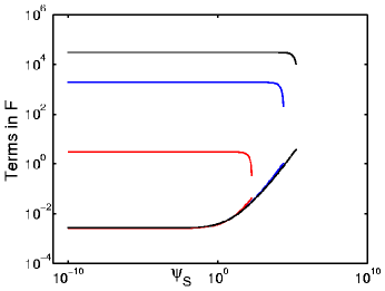
Figure 1: The values of $F_{I}+F_{O}$ (top three curves) and $\hat{F}$ (the highly overlapping bottom curves) as a function of the rescaled mass parameter $\psi_{S}$ over the range $10^{-10}<\psi_{S}<\psi_{cr}$.The three values of the pair ($m_{I}/m_{P}$,$\lambda$) shown here are given by ($0.5$,$33.5$), ($0.1$,$838$), and ($0.05$,$3350$) in order of increasing $\psi_{cr}$. The main point of this figure is that $F_{I}+F_{O}\gg\hat{F}$ for all relevant values of $\psi_{S}$ for any realistic value of $\lambda$. More detailed features of this plot are discussed in the text.

In bgg it is also shown that the turning point solutions do not exist for $M>M_{cr}$. In that regime there is no tunneling and no chance to produce inflation. Like $M_{S}$ and $M_{D}$, $M_{cr}$ also takes the form $M_{cr}=\bar{M}(1+O(1/\lambda))$. For realistic models of inflation $m_{I}\leq O(10^{-2.5})m_{P}$, so again taking $\mu\approx m_{I}^{3}$, $1/\lambda\ll 1$. Thus for realistic models, $M<M_{D}$ holds for all $M$ except for a tiny range $\Delta M\approx\bar{M}/\lambda$ near the maximum value $M_{cr}\approx\bar{M}$. The form of $P_{c}$ dictates that minimum values of $M$ are the relevant ones, so we can use the $M<M_{D}$ part of Eqn. 31 for $F_{I}+F_{O}$ in $P_{q}$ for all values of $M$ without producing any significant errors.

Figure 1 shows $F_{I}+F_{O}$ and $\hat{F}$ for three different values of $m_{I}$ (and $\lambda$, which we take to be specified uniquely from $m_{I}$ by using $\mu=m_{I}^{3}$ in Eqn. 35). We’ve chosen unrealistically large values of $m_{I}$ so that key features can be shown more easily on the plot. The pair of curves corresponding to each value of $m_{I}$ extends all the way to the maximal value of $\psi_{S}=\psi_{cr}\equiv\psi_{S}(M_{cr})=\lambda^{3/2}(1+O(1/\lambda))$ corresponding to the given value of $m_{I}$ .

We see that the $M\rightarrow 0$ limit is a good approximation for $\hat{F}$ for values of $\psi_{S}$ up to $\psi_{S}\approx 1$. Above $\psi_{S}=1$, $\hat{F}$ increases, but remains orders of magnitude smaller than $F_{I}+F_{O}$ except possibly in the tiny (unresolved) region near the maximal value $\psi_{cr}$. Note that the $\hat{F}$ curves coincide (over their defined ranges) except for corrections $O(1/\lambda)$ which are barely visible on this plot due to the (large) chosen values of $\lambda$.

As discussed in Section IV, the most significant values of $P_{q}$ are those corresponding to masses given by the cutoff value $m_{l}$ (which we expressed in terms of the corresponding black hole entropy $S_{l}$). The corresponding cutoff value of $\psi_{S}$ is given by $\psi_{l}=\sqrt{S_{l}/S_{I}}\lambda^{3/2}\approx\sqrt{S_{S}/S_{I}}\psi_{cr}$. One can see from Fig. 1 that with the possible exception of values of $\psi_{l}$ extremely close to $\psi_{cr}$ (over a region too narrow to resolve on this plot), $F\approx F_{I}+F_{O}$ will be an excellent approximation for the purposes of our calculations. Since the maximum value of the cutoff proposed here gives $S_{l}=\sqrt{S_{I}}$, $\psi_{l}\ll\psi_{cr}$ so we are always considering values well away from the narrow $\psi_{S}\approx\psi_{cr}$ zone. Even at the closest approach shown $\hat{F}\ll F_{I}+F_{O}$, and the gap widens with decreasing $m_{I}$. Thus throughout this paper we take

$$F=F_{I}+F_{O}=\frac{\pi}{2\,G}\,\left(R_{I}^{2}-R_{S}^{2}\right)\approx\frac{\pi}{2\,G}R_{I}^{2}.$$ (42)

in $P_{q}$.

Appendix B Relationship to issues raised by Penrose and others

There is some connection between our discussion here and conceptual issues that have been discussed over some time in connection with inflation, especially the work of Page Page:1983uh (in responding to Davies Davies:1983nf ) and later Penrose Penrose , Unruh Unruh and Hollands and Wald Hollands:2002xi . Page and Penrose emphasize the point that initial conditions which given the big bang a thermodynamic arrow of time must necessarily be low entropy and therefore “rare”. There is no way the initial conditions can be typical, or there would be no arrow of time, and this fact must apply to inflation and prevent it from representing “completely generic” initial conditions.

The position we take here (which was suggested by Davies in Davies:1984qc and is the same one taken by DKS and emphasized at length in Albrecht:2002uz ) is basic acceptance of this point. If you can regard the big bang as a fluctuation in a larger system it must be an exceedingly rare one to account for the observed thermodynamic arrow of time. Also, we believe that this is the most attractive possibility for a theory of initial conditions. Other theories of initial conditions seem to us more ad hoc, and less compelling.

There is an additional point that appears in Unruh and Hollands:2002xi , but which many (including one of us, AA) recall also being discussed orally (but apparently not in print) by Penrose: It might be argued that inflation, which has a lower entropy initial state than the big bang must necessarily be more rare than a fluctuation giving a big bang without inflation. For a number of reasons this point of view never really caught on. One reason is that intuitively it seemed likely that a careful accounting of degrees of freedom outside the observed universe would reverse that conclusion. Hollands and Wald specifically note this view, although they also seem drawn to the Penrose argument.

All these issues play out in this paper, but in a more concrete form. DKS have a specific reason why they ignore the external degrees of freedom (there aren’t any separate external degrees of freedom in the causal patch analysis). DKS are able to quantify the serious problems this causes for inflation. Our calculation explicitly does account for external degrees of freedom and we show quantitatively that that change does indeed reverse the fortunes of inflation.

References

- (1) A. Guth, Phys. Rev. D 23, 347 (1981); A. Linde, Phys. Lett. B 108, 389 (1982); A. Albrecht and P. Steinhardt, Phys. Rev. Lett. 48, 1220 (1982).
- (2) H. V. Peiris et al., Astrophys. J. Suppl. 148 (2003) 213 [arXiv:astro-ph/0302225].
- (3) A. Vilenkin, Phys. Lett. B 117 (1982) 25.
- (4) J. B. Hartle and S. W. Hawking, Phys. Rev. D 28, 2960 (1983).
- (5) E. Farhi and A. H. Guth, Phys. Lett. B 183 (1987) 149.
- (6) A. D. Linde, Nucl. Phys. B 372, 421 (1992) [arXiv:hep-th/9110037].
- (7) A. Linde, Phys. Lett. B 129, 177 (1983).
- (8) J. Garriga and A. Vilenkin, Phys. Rev. D 57, 2230 (1998) [arXiv:astro-ph/9707292].
- (9) L. Dyson, M. Kleban and L. Susskind, JHEP 0210 (2002) 011 [arXiv:hep-th/0208013].
- (10) S. W. Hawking and T. Hertog, Phys. Rev. D 66 (2002) 123509 [arXiv:hep-th/0204212].
- (11) N. Turok, arXiv:astro-ph/0011195.
- (12) N. Turok, Class. Quant. Grav. 19 (2002) 3449.
- (13) S. Hawking, arXiv:astro-ph/0305562. Talk presented at Davis Inflation Meeting, 2003 (astro- ph/0304225)
- (14) A. Albrecht, “Cosmic inflation and the arrow of time,” arXiv:astro-ph/0210527. In ”Science and Ultimate Reality: From Quantum to Cosmos”, honoring John Wheeler’s 90th birthday. J. D. Barrow, P.C.W. Davies, & C.L. Harper eds. Cambridge University Press (2004)
- (15) D. H. Coule, Int. J. Mod. Phys. D 12 (2003) 963 [arXiv:gr-qc/0202104].
- (16) T. Banks, W. Fischler and S. Paban, JHEP 0212 (2002) 062 [arXiv:hep-th/0210160].
- (17) This work builds on the discussion presented in a talk by one of us (AA) at the “KITP superstring cosmology workshop” (October 2003) http://online.kitp.ucsb.edu/online/strings03/
- (18) T. Banks, hep-th/0007146; hep-th/0011255; T. Banks and W. Fischler, hep-th/0102077.
- (19) S. Hellerman, N. Kaloper and L. Susskind, JHEP 0106 (2001) 003; W. Fischler, A. Kashani-Poor, R. McNees and S. Paban, JHEP 0107 (2001) 003.
- (20) E. Witten, hep-ph/0002297.
- (21) W. Fischler and L. Susskind, hep-th/9806039.
- (22) R. Bousso, JHEP 9907 (1999) 004; JHEP 9906 (1999) 028; JHEP 0011 (2000) 038.
- (23) G. W. Gibbons and S. W. Hawking, Phys. Rev. D 15, 2738 (1977).
- (24) A. D. Linde, Phys. Lett. B 175, 395 (1986).
- (25) A. Vilenkin, Phys. Rev. D 27, 2848 (1983). A. H. Guth, In the proceedings of the Cosmic Questions Conference, Washington, DC Apr 1999, New York Academy of Sciences Press. arXiv:astro-ph/0101507.
- (26) L. Susskind, arXiv:hep-th/0302219.
- (27) For a nice discussion of this paradox see J. Barrow and F. Tipler, “The anthropic cosmological principle”, Oxford University Press (1986)
- (28) W. Fischler, D. Morgan and J. Polchinski, Phys. Rev. D 41 (1990) 2638. W. Fischler, D. Morgan and J. Polchinski, Phys. Rev. D 42 (1990) 4042.
- (29) E. Farhi, A. H. Guth and J. Guven, Nucl. Phys. B 339, 417 (1990).
- (30) S. K. Blau, E. I. Guendelman and A. H. Guth, Phys. Rev. D 35, 1747 (1987).
- (31) D. N. Page, Nature 304 (1983) 39.
- (32) P. C. W. Davies, Nature 301 (1983) 398.
- (33) R. Penrose in Proc. 14th Texas Symp. on Relativistic Astrophysics E. J. Fergus ed., New York Academy of Sciences, 249 (1989).
- (34) W. Unruh in Critical Dialogs in Cosmology N. Turok ed. p249 World Scientific (1997).
- (35) S. Hollands and R. M. Wald, arXiv:hep-th/0210001.
- (36) P. C. W. Davies, Nature 312 (1984) 524.