NORDITA-2004-42

PAR-LPTHE 04-011

We analyse the renormalisation properties of composite operators of scalar fields in the ${\cal N}=2$ Super Yang–Mills theory. We compute the matrix of anomalous dimensions in the planar limit at one–loop order in the ’t Hooft coupling, and show that it corresponds to the Hamiltonian of an integrable XXZ spin chain with an anisotropy parameter $\Delta>1$. We suggest that this parameter could be related to the presence of non–trivial two–form fluxes in the dual supergravity background. We find that the running of the gauge coupling does not affect the renormalization group equations for these composite operators at one–loop order, and argue that this is a general property of gauge theories which is not related to supersymmetry.

1 Introduction

The study of the AdS/CFT correspondence in the PP–wave limit (for a review, see [1, 2, 3, 4, 5]) has triggered a great deal of work in the renormalisation properties of composite operators in gauge theory. The original idea of Berenstein, Maldacena and Nastase [6] was to regard some gauge–invariant operators of the ${\cal N}=4$ Super Yang–Mills theory having large $R$–charge as a discretised version of the physical type IIB string on the PP–wave background. The BMN operators are single trace operators formed by a long chain of one of the elementary scalar fields of ${\cal N}=4$, with the insertion of a few other fields and covariant derivatives (called impurities), each of them corresponding to a different excitation of the string. The anomalous dimensions of these operators is expected to coincide with the mass of the corresponding string state [6]. This matching was first checked perturbatively at one-loop [6] and at two-loop [7] level, and then a field theory argument was provided in [8] to extend the correspondence to all orders of perturbation theory.

In [9] it was realised that the string theory states accessible by quantization on the plane–wave background are indeed a subsector of a wider class of highly excited string states which can be described as semiclassical soliton solutions of the AdS${}_{5}\times$S⁵ string sigma model. The general feature of these states is that they carry large quantum numbers, corresponding to large angular momenta along the five sphere and/or the AdS space. The AdS/CFT dictionary enables one to identify the corresponding gauge theory operators. As in the BMN case, they are built as a long chain of elementary fields, but in this case with an high number of impurities. The computation of the anomalous dimensions of such operators is in general a formidable task, due to the large number of different fields that they contain.

A very interesting observation was made in [10], where the matrix of the one–loop anomalous dimensions for the composite operators of scalar fields of ${\cal N}=4$ SYM theory in the planar limit was put in correspondence with the Hamiltonian of an integrable $SO(6)$ spin chain. This inspired further studies on the integrability of the planar ${\cal N}=4$ theory SYM at one–loop [11, 12, 13, 14] and also at higher orders [15, 16, 17, 18, 19, 20]. The relation with the integrable systems allows one to compute the anomalous dimensions of the “long” gauge theory operators by using the algebraic Bethe ansatz. In general, for states that have at least one large angular momentum $J$ along the five sphere, as for the plane–wave states, one can define an effective expansion parameter $\lambda^{\prime}=\lambda/J^{2}$. In some cases, as for the BMN operators, both the semiclassical expansion of string theory and the perturbative expansion in gauge theory can be defined in terms of this effective parameter, allowing for a quantitative comparison between the two. Several studies have been performed along these lines and agreement has been found up to two loops. One salient feature of these developments is that they allow one to probe regions of the string spectrum far away from the states protected by supersymmetry. It is a remarkable fact that one finds a quantitative agreement also in these cases. It is thus conceivable that similar patterns of gauge/string duality can be unraveled also for theories where some (or all) the supersymmetries are broken [22] and the conformal invariance is lost [23, 24, 25].

Studies on the integrability in deformed ${\cal N}=4$ SYM theories were performed in [26], which considered the Leigh–Strassler deformation, in [27, 28], where the ${\cal N}=2,1$ orbifold field theories were considered, and in [29] in the context of defect conformal field theories. A general study on the integrability of ${\cal N}=4$ SYM in presence of marginal deformations has been recently presented in [30].

In this paper, we focus our attention on the pure ${\cal N}=2$ SYM theory, and we study the renormalisation properties of composite operators of scalar fields. We find that the corresponding matrix of the anomalous dimensions reduces at one–loop and in the planar limit to the Hamiltonian of an XXZ spin chain. We also study the renormalisation group flow for these operators and show that the effects of the breaking of the conformal invariance show up only at the two–loop order in the ’t Hooft coupling.

2 ${\cal N}=2$ theory and the XXZ spin chain

We start by writing the Lagrangian of ${\cal{N}}=2$ Super Yang-Mills in Weyl notations

$$L_{E} = \frac{2}{g^{2}}{\rm Tr}\Big{(}\frac{1}{4}F_{\mu\nu}F_{\mu\nu}+(D_{\mu}\phi)^{\dagger}D_{\mu}\phi+\psi\sigma^{\mu}D^{\mu}\bar{\psi}+\lambda\sigma^{\mu}D^{\mu}\bar{\lambda}$$ (1)

$$-i\sqrt{2}\left(\psi[\bar{\phi},\lambda]+\bar{\psi}[\phi,\bar{\lambda}]\right)+\frac{1}{2}[\bar{\phi},\phi]^{2}\Big{)}\ ,$$

in terms of the euclidean $\sigma$-matrices $\sigma^{\mu}=({\bf 1},i\tau^{i})$. The field $\phi$ is the complex scalar of the ${\cal N}=2$ Super Yang-Mills, the two Weyl spinors $\lambda$ and $\psi$ are the fermionic superpartners and the covariant derivative reads $D_{\mu}\phi=\partial_{\mu}\phi-i[A_{\mu},\phi]$.

Let us start by studying the renormalization properties of operators involving a product of the complex scalar field $\phi$ 

$$G_{J}(x_{1},\ldots,x_{J};z)={\cal Z}_{\phi}^{J/2}\langle\bar{\phi}_{r}(x_{1})\ldots\bar{\phi}_{r}(x_{J}){\cal Z}_{{\cal O}}{\rm Tr}(\phi^{J})_{r}(z)\rangle={\cal Z}_{\phi}^{J/2}{\cal Z}_{{\cal O}}G_{J}^{(ren)}(x_{1},\ldots,x_{J};z)$$ (2)

${\cal Z}_{{\cal O}}$ is the renormalization factor for the composite operator, and ${\cal Z}_{\phi}$ is the usual wave–function renormalization needed to make finite the two–point function $\langle\bar{\phi}_{r}(x)\phi_{r}(y)\rangle$. Notice that the product of the fields ${\bar{\phi}}\equiv\bar{\phi}^{a}(T^{a})_{ij}$ in the Green function (2) should be understood as a product of the gauge group matrices. This means that the Green function is a matrix, but sometimes we will not write explicitly its indices in order to avoid a too heavy formalism. The factor ${\cal Z}_{{\cal O}}$ is defined in order to reabsorb all the divergencies arising in the computation of the bare correlator $G_{J}$ in (2) with the Lagrangian (1). It turns out that in ${\cal{N}}=2$ Super Yang-Mills all the self-energy diagrams cancel. This means that in the convention we choose for the lagrangian (1) the only renormalization for the fields is that associated to the gauge coupling, i.e. ${\cal Z}_{\phi}^{1/2}\equiv{\cal Z}_{g}$. On the other hand from the knowledge of the $\beta$-function

$$\beta(g)\equiv\mu\frac{\partial}{\partial\mu}g_{r}=-g\mu\frac{\partial}{\partial\mu}\log{\cal Z}_{g}=-\frac{g^{3}}{16\pi^{2}}2N$$ (3)

one can derive the expression for ${\cal Z}_{g}$

$${\cal Z}_{g}=1-\frac{g^{2}N}{16\pi^{2}}\frac{\mu^{-2\epsilon}}{\epsilon}\ .$$ (4)

Indeed (3) follows from (4) after taking the $\epsilon\to 0$ limit.

We are now ready to study the renormalization properties of the composite operator in (2). For the sake of clarity we start by considering the case $J=2$

$$G_{2}(x,y;z)\equiv\langle(\bar{\phi}(x)\bar{\phi}(y))_{ij}{\rm Tr}(\phi^{2})(z)\rangle\ .$$ (5)

The tree level contribution in the planar limit is

$$G_{2}(x,y;z)|_{tree}=\langle(\bar{\phi}(x)\bar{\phi}(y))_{ij}{\rm Tr}(\phi^{2})(z)\rangle_{\rm tree}=g^{4}\frac{N}{2}\Delta_{xz}\Delta_{yz}\delta_{ij}$$ (6)

where we have used the scalar field propagator

$$\langle{\bar{\phi}}_{ij}(x)\phi_{hk}(y)\rangle=\frac{g^{2}}{2}\left(\delta_{ik}\delta_{jh}\ -\frac{1}{N}\delta_{ij}\delta_{hk}\right)\Delta_{xy}$$ (7)

with

$$\Delta_{xy}\equiv\int\frac{d^{2\omega}p}{(2\pi)^{2\omega}}\frac{e^{ip\cdot(x-y)}}{p^{2}}=\frac{\Gamma(\omega-1)}{4\pi^{\omega}(|x-y|^{2})^{\omega-1}}\ .$$ (8)

We use dimensional regularization with the dimension of the space-time equal to $2\omega\equiv 4-2\epsilon$. At one-loop the previous correlator has two contributions: one coming from the scalar potential and the second coming from the gluon exchange. In principle there could be also the contribution of the self-energy diagrams that, however, cancels as we have already remarked.

Figure 1: Feynman diagrams contributing at one–loop. The thick horizontal line joins the fields belonging to the composite operator.

In the planar limit we get

$$G_{2}(x,y;z)|_{1-loop;planar}=G_{2}(x,y;z)|_{tree}\times g^{2}N\left(K(z;x,y)+{\cal G}(z;x,y)\right)$$ (9)

where

$$K(z;x,y)\equiv\Delta_{xz}^{-1}\Delta_{yz}^{-1}\int d^{2\omega}u\Delta_{xu}(\Delta_{zu})^{2}\Delta_{yu}\sim\frac{1}{16\pi^{2}}\left(\frac{1}{\epsilon}+\dots\right)$$ (10)

and

$${\cal G}(z;x,y)=\Delta^{-1}_{zy}\Delta^{-1}_{zx}\int d^{2\omega}y_{1}\int d^{2\omega}y_{2}(\Delta_{zy_{1}}\stackrel{{\scriptstyle\leftrightarrow}}{{\partial_{\mu}}}^{y_{1}}\Delta_{y_{1}x})(\Delta_{zy_{2}}\stackrel{{\scriptstyle\leftrightarrow}}{{\partial_{\mu}}}^{y_{2}}\Delta_{y_{2}y})\Delta_{y_{1}y_{2}}\sim$$

$$\sim\frac{1}{16\pi^{2}}\left(\frac{1}{\epsilon}+\dots\right)\ .$$ (11)

The symbol $\stackrel{{\scriptstyle\leftrightarrow}}{{\partial_{\mu}}}$ in (11) stands for the left–right derivative $(A\stackrel{{\scriptstyle\leftrightarrow}}{{\partial_{\mu}}}B)=A\partial_{\mu}B-\partial_{\mu}AB$. The fastest way to get the planar contribution in the correlator containing the string of fields ${\bar{\phi}}$ and a product of various traces is first to perform all the possible contractions that reduce everything to a single string of fields and then contract only the fields that are next to each other in this single string. This procedure maximizes the number of factors $N$ and gives the planar contribution. Both in (10) and (11) we have kept only the divergent terms that are the ones that we need, while the dots represent the finite parts. Eq.(9) can be easily generalized, at the planar level, to arbitrary $J$

$$G_{J}(x_{1}\ldots x_{i},x_{i+1}\ldots x_{J};z)|_{1-loop;planar}=$$

$$=G_{J}(x_{1}\ldots x_{i},x_{i+1}\ldots x_{J};z)|_{tree;planar}\sum_{i=1}^{J}\frac{g^{2}N}{2}\left[K(z;x_{i},x_{i+1})+{\cal G}(z;x_{i},x_{i+1})\right]\sim$$

$$\sim G_{J}(x_{1}\ldots x_{J};z)|_{tree}\times g^{2}N\frac{J}{16\pi^{2}}\frac{\mu^{-2\epsilon}}{\epsilon}$$ (12)

where $(x_{i},x_{i+1})$ are two nearest–neighbors fields in the correlator and

$$G_{J}(x_{1},x_{2},\dots x_{J};z)_{tree,planar}=\frac{JN^{J-1}g^{2J}}{2^{J}}\delta^{ij}\Delta_{x_{1}z}\Delta_{x_{2}z}\dots\Delta_{x_{J}z}$$ (13)

In the last term of (12) we wrote the divergent terms, coming half from the gluon exchange and half from the four scalar interaction. Collecting the tree–level and the one loop contributions together we have

$$G_{J}(x_{1}\ldots x_{J};z)_{one-loop;planar}=G_{J}(x_{1}\ldots x_{J};z)|_{tree;planar}\left(1+g^{2}N\frac{J}{16\pi^{2}}\frac{\mu^{-2\epsilon}}{\epsilon}\right)$$ (14)

Finally, by converting the bare coupling factor $g^{2J}$ appearing in $G_{J}|_{tree}$ into the renormalised coupling $g_{r}^{2J}$, (14) gets a factor ${\cal Z}_{g}^{2J}$. If we now consider the renormalized correlator in (2), by using (4) we see that the divergence appearing in (14) is exactly cancelled by the renormalization factors ${\cal Z}_{\phi}^{-J/2}{\cal Z}_{g}^{2J}={\cal Z}_{g}^{J}$, without the need of any renormalization constant for the composite operator, i.e. ${\cal Z}_{{\cal O}}=1$. This means that these operators are protected at one–loop. Indeed, in [31, 32, 33, 34] it was shown that the generalised Slavnov–Taylor identities associated to the ${\cal N}=2$ supersymmetry imply that these operators have vanishing anomalous dimensions to all orders in perturbation theory. The above computation provides an explicit check of this property at one–loop.

Let us now come to the more general case of composite operators of the two real scalar fields of the ${\cal N}=2$ theory

$${\cal O}={\rm Tr}\left(\varphi_{i_{1}}\ldots\varphi_{i_{l}}\varphi_{i_{l+1}}\ldots\varphi_{i_{L}}\right)\ ,$$ (15)

where

$$\phi=\frac{1}{\sqrt{2}}\left(\varphi_{1}+i\varphi_{2}\right)\ .$$ (16)

We derive the one-loop planar mixing matrix for anomalous dimensions following very closely the procedure used in [10] for ${\cal{N}}=4$. We then study the correlator

$$\langle\varphi^{i_{L}}\ldots\varphi^{i_{l+1}}\varphi^{i_{l}}\ldots\varphi^{i_{1}}{\cal O}\rangle={\cal Z}_{\varphi}^{L/2}{\cal Z}_{\cal O}\langle\varphi^{i_{L}}_{r}\ldots\varphi^{i_{l+1}}_{r}\varphi^{i_{l}}_{r}\ldots\varphi^{i_{1}}_{r}{\cal O}_{r}\rangle$$ (17)

where $\varphi={\cal Z}_{\varphi}^{1/2}\varphi_{r}$ and ${\cal Z}_{\varphi}={\cal Z}_{\phi}$ by virtue of (16). The operators (15) mix among themselves at the quantum level, and ${\cal Z}_{\cal O}$ is a matrix carrying the indices of the real fields. One can wonder whether the set of operators (15) is closed under renormalization. First of all, one can easily see that the one–loop diagrams in which two real fields of the operator (15) combine to emit a gluon or a fermionic current are vanishing for symmetry reasons. Then the only remaining possibility is a mixing with scalars operators containing derivatives. These operators do indeed appear in the counterterms needed for the renormalisation of the operators (15) [35]. However, the converse is not true, since the operators (15) do not appear as counterterms in the one–loop renormalisation of operators containing derivatives. This implies that the mixing matrix is triangular and one can disregard the mixing with derivative operators as far as the computation of the one–loop anomalous dimensions is concerned. We need then to study only the correlators (17). By using the large $N$ approximation, we focus on the nearest–neighbors interaction

$$\langle\ldots\varphi_{i_{l+1}}(x)\varphi_{i_{l}}(y)\ldots{\rm Tr}\Big{(}\ldots\varphi_{j_{l}}\varphi_{j_{l+1}}\ldots\Big{)}(z)\rangle$$ (18)

The one–loop correction associated to the gluon exchange is exactly the same as that for the complex fields, and can be read from the last line of (12) by taking only half the contribution as explained just after (12). By introducing also the (diagonal) index structure of the real scalar fields, we get

$${\cal Z}^{(gluon)\ldots j_{l}j_{l+1}\ldots}_{\ \ \ldots i_{l}i_{l+1}\ldots}={\bf 1}+\frac{g^{2}N}{16\pi^{2}}\frac{\mu^{-2\epsilon}}{2\epsilon}\ \delta_{i_{l}}^{j_{l}}\delta_{i_{l+1}}^{j_{l+1}}\ \ .$$ (19)

In order to compute the contribution of the four-scalar interaction, it is convenient to rewrite it in terms of real scalars

$$V_{4}=-\frac{1}{2g^{2}}\sum_{i,j=1}^{2}{\rm Tr}\left([\varphi_{i},\varphi_{j}][\varphi_{i},\varphi_{j}]\right)$$ (20)

The correction associated to four scalar interaction (20) is

$$\langle\varphi_{i_{l+1}}(x)\varphi_{i_{l}}(y)\times$$

$$\int d^{2\omega}u\frac{1}{2g^{2}}{\rm Tr}\Big{[}\sum_{l,m=1}^{2}\Big{(}2\varphi_{l}\varphi_{m}\varphi_{l}\varphi_{m}-\varphi_{l}\varphi_{m}\varphi_{m}\varphi_{l}-\varphi_{l}\varphi_{l}\varphi_{m}\varphi_{m}\Big{)}\Big{]}(u){\rm Tr}\Big{(}\varphi_{j_{l}}\varphi_{j_{l+1}}\Big{)}(z)\rangle$$

$$=g^{4}\frac{N}{2^{2}}\Delta_{xz}\Delta_{yz}\times\frac{g^{2}}{2}\frac{N}{2^{2}}\ 4K(z;x,y)\Big{(}2\delta_{i_{l}}^{j_{l+1}}\delta^{j_{l}}_{i_{l+1}}-\delta_{i_{l}}^{j_{l}}\delta_{i_{l+1}}^{j_{l+1}}-\delta_{i_{l}i_{l+1}}\delta^{j_{l}j_{l+1}}\Big{)}$$

$$\sim g^{4}\frac{N}{2^{2}}\Delta_{xz}\Delta_{yz}\times\frac{g^{2}N}{16\pi^{2}}\frac{\mu^{-2\epsilon}}{2\epsilon}\ \Big{(}2\delta_{i_{l}}^{j_{l+1}}\delta^{j_{l}}_{i_{l+1}}-\delta_{i_{l}}^{j_{l}}\delta_{i_{l+1}}^{j_{l+1}}-\delta_{i_{l}i_{l+1}}\delta^{j_{l}j_{l+1}}\Big{)}\ ,$$ (21)

The factor $N/2^{2}$ appearing in the second line of (21) is associated to the matrix contractions and the factor $4$ comes from the four possible contractions with the fields in the vertex. The ${\cal Z}$ factor associated to the above correction is

$${\cal Z}^{(four\ sc.)\ldots j_{l}j_{l+1}\ldots}_{\ \ \ldots i_{l}i_{l+1}\ldots}={\bf 1}+\frac{g^{2}N}{16\pi^{2}}\frac{\mu^{-2\epsilon}}{2\epsilon}\ \Big{(}2\delta_{i_{l}}^{j_{l+1}}\delta^{j_{l}}_{i_{l+1}}-\delta_{i_{l}}^{j_{l}}\delta_{i_{l+1}}^{j_{l+1}}-\delta_{i_{l}i_{l+1}}\delta^{j_{l}j_{l+1}}\Big{)}\ .$$ (22)

In conclusion the contributions coming from the gluon exchange and from the four-scalar interaction are the same as in the ${\cal{N}}=4$ case [10] except that now the indices $i_{l},i_{l+1},j_{l},j_{l+1}$ run only over two values and not six because ${\cal{N}}=2$ Super Yang-Mills has only two real scalars. In addition in ${\cal{N}}=4$ we have also the contribution of the self-energy diagrams. In the ${\cal{N}}=2$ case, as we already remarked, there are instead no self–energy corrections and the renormalization of the fields is given at one–loop by the coupling constant ${\cal Z}_{g}$–factor. More precisely, in (17) it appears the factor ${\cal Z}_{\varphi}^{L/2}={\cal Z}_{g}^{L}$. To pass from the bare coupling $g^{2L}$ appearing in the bare correlator in (17) to the renormalised one we still have to multiply the r.h.s. of (17) by a ${\cal Z}_{g}$ factor for each field. This amount to the following renormalisation factor for the nearest–neighbors

$${\cal Z}^{(g)\ldots j_{l}j_{l+1}\ldots}_{\ \ \ldots i_{l}i_{l+1}\ldots}={\bf 1}-\frac{g^{2}N}{8\pi^{2}}\frac{\mu^{-2\epsilon}}{2\epsilon}\ \delta_{i_{l}}^{j_{l}}\delta_{i_{l+1}}^{j_{l+1}}\ \ .$$ (23)

Adding the three contributions in (19), (22) and (23) we get

$${\cal{Z}}^{\ldots j_{l}j_{l+1}\ldots}_{\ \ \ldots i_{l}i_{l+1}\ldots}={\bf 1}-\frac{g^{2}N}{16\pi^{2}}\frac{\mu^{-2\epsilon}}{2\epsilon}\left(\delta_{i_{l}i_{l+1}}\delta^{j_{l}j_{l+1}}+2\delta_{i_{l}}^{j_{l}}\delta_{i_{l+1}}^{j_{l+1}}-2\delta_{i_{l}}^{j_{l+1}}\delta^{j_{l}}_{i_{l+1}}\right)\ .$$ (24)

The resulting matrix of anomalous dimensions for these operators turns out to be the same as in ${\cal N}=4$ theory [10], except that now the indices run only over the values $1$ and $2$ . For the particular case of the composite operators of complex fields in (2), the matrix is vanishing, in agreement with the result discussed after (12). In fact these operators, when represented in terms of the real fields $\varphi_{i}$, are symmetric and traceless in the real indices $i=1,2$, and this ensures the vanishing of their one–loop anomalous dimensions computed from (24). In this sense, these operators are the analogous in the ${\cal N}=2$ theory of the BPS (or chiral primary) operators of the ${\cal N}=4$ SYM [31, 32, 33, 34].

As another example, one can consider the Konishi operator ${\cal K}={\rm Tr}\bar{\phi}\phi$. In the direct computation of the planar, one–loop renormalisation of this operator one finds that the contribution of the gluon exchange has the opposite sign with respect to that of the four scalar interaction. Thus they cancel out and the only renormalisation of the Konishi operator is that associated to the gauge coupling: ${\cal Z}_{\cal K}={\cal Z}_{g}^{2}$. From this it follows that $\gamma_{\cal K}=\lambda/4\pi^{2}$. On the other side, when one acts on ${\cal K}$ with the matrix (24), the contributions of the identity and of the permutation operators compensate each other and only the trace contribution is left. By summing on the two sites and using (4) one gets again ${\cal Z}_{\cal K}={\cal Z}_{g}^{2}$, in agreement with the direct computation.

Let us now come to the discussion of the relation with the spin chain. Quite naturally the two scalar fields of the ${\cal N}=2$ SYM can be interpreted as different orientations of a spin and then the whole gauge invariant operator formed just by scalars can be seen as a spin chain. The cyclicity of the trace makes the chain closed and implies that the physical states of the chain corresponding to the gauge theory operators have zero total momentum.

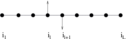
\begin{picture}(0.0,0.0)\end{picture}

Figure 2: Spin chain

From this point of view, we can interpret the matrix of the one-loop anomalous dimensions

$$\gamma_{\cal O}\equiv{\cal Z}_{\cal O}^{-1}\mu\frac{\partial}{\partial\mu}{\cal Z}_{\cal O}$$ (25)

which we get from (24)

$$\gamma_{\cal O}=\frac{g^{2}N}{16\pi^{2}}\sum_{l=1}^{L}\left(K_{l,l+1}+2-2P_{l,l+1}\right)=\frac{\lambda}{16\pi^{2}}\sum_{l=0}^{L}H_{l,l+1}$$ (26)

as a Hamiltonian acting on the spin chain. Since the indices of the real scalar fields of the ${\cal N}=2$ theory run just from one to two, we can directly rewrite the matrix of anomalous dimensions (26) in the basis of sigma matrices $\hat{\sigma}_{\mu}\equiv({\bf 1},\hat{\sigma}^{x},\hat{\sigma}^{y},\hat{\sigma}^{z})$ which is better suited for the study of spin chain systems. In this basis $\varphi_{1}\rightarrow(1\,\,0)$ and $\varphi_{2}\rightarrow(0\,\,1)$. The permutation operator is

$$P^{j_{l}j_{l+1}}_{i_{l}i_{l+1}}\equiv\delta_{i_{l}}^{j_{l+1}}\delta_{i_{l+1}}^{j_{l}}=\frac{1}{2}\sum_{\mu=0}^{3}\beta_{\mu}(\hat{\sigma}^{\mu})^{j_{l}}_{~{}~{}i_{l}}(\hat{\sigma}^{\mu})^{j_{l+1}}_{~{}~{}i_{l+1}}\ ,$$ (27)

with coefficients $\beta_{\mu}=(1,1,1,1)$, and the “trace” contribution, where the two consecutive real fields are equal, is

$$K^{j_{l}j_{l+1}}_{i_{l}i_{l+1}}\equiv\delta_{i_{l}i_{l+1}}\delta^{j_{l}j_{l+1}}=\frac{1}{2}\sum_{\mu=0}^{3}\alpha_{\mu}({\hat{\sigma}}^{\mu})^{j_{l}}_{~{}i_{l}}({\hat{\sigma}}^{\mu})^{j_{l+1}}_{~{}~{}i_{l+1}}$$ (28)

where $\alpha_{\mu}=(1,1,-1,1)$. Moreover, before to write down the spin chain Hamiltonian we observe that the operators containing only products of the complex scalar field $\phi$ have vanishing anomalous dimensions. This suggest to take them as the lowest energy eigenstates of the spin chain and to identify the two orientations of a spin with the following $2$-vectors

$$\bar{\phi}\to|+\rangle\equiv\left(\begin{array}[]{c}1\\ 0\end{array}\right)~{}~{},~{}~{}~{}~{}\phi\to|-\rangle\equiv\left(\begin{array}[]{c}0\\ 1\end{array}\right)~{}.$$ (29)

From (16) one immediatly realises that the change of basis required to satisfy (29) has to exchange the two Pauli matrices $\hat{\sigma}^{y}\to-\sigma^{z}$ and $\hat{\sigma}^{z}\to\sigma^{y}$ leaving unchanged the third $\hat{\sigma}^{x}\to\sigma^{x}$. The action of the Pauli matrices in the basis (29) is $\sigma^{x}|+\rangle=|-\rangle$, $\sigma^{x}|-\rangle=|+\rangle$, $\sigma^{y}|+\rangle=i|-\rangle$, $\sigma^{y}|-\rangle=-i|+\rangle$, $\sigma^{z}|+\rangle=|+\rangle$ and $\sigma^{z}|-\rangle=-|-\rangle$, and the matrix of anomalous dimensions (26) reads

$$\gamma_{\cal O} = -\frac{g^{2}N}{32\pi^{2}}\sum_{l=1}^{L}\left[(\sigma^{x})_{l}(\sigma^{x})_{l+1}+(\sigma^{y})_{l}(\sigma^{y})_{l+1}+3\left((\sigma^{z})_{l}(\sigma^{z})_{l+1}-{\bf 1}_{l}{\bf 1}_{l+1}\right)\right]$$ (30)

$$\equiv \frac{\lambda}{16\pi^{2}}H_{\rm XXZ}\ ,$$

where

$$H_{\rm XXZ}=-\frac{1}{2}\sum_{l=1}^{L}\left[(\sigma^{x})_{l}(\sigma^{x})_{l+1}+(\sigma^{y})_{l}(\sigma^{y})_{l+1}+3\left((\sigma^{z})_{l}(\sigma^{z})_{l+1}-{\bf 1}_{l}{\bf 1}_{l+1}\right)\right]$$ (31)

is the Hamiltonian of an XXZ spin system!![36]. An interesting feature of this system is that it displays an anisotropy parameter $\Delta$. The behaviour of the spin chain depends critically on the value of this parameter; in particular for $\Delta>1$ the spectrum has a mass gap [36]. The integrable system that we find in the ${\cal N}=2$ case belongs to this class, since from (31) we read $\Delta=3$. As anticipated, the ground state of the spin chain corresponds to the protected operator ${\cal O}_{vac}\equiv{\rm Tr}(\phi^{L})$. The excited states are associated to spin flips along the chain, which in the field theory language correspond to the insertion of “impurities” $\bar{\phi}$ in the operator ${\cal O}_{vac}$. Due to the constraint of zero total momentum imposed by the cyclicity of the trace, we have to consider at least two impurities, i.e. we study the operator

$${\cal O}_{n}=\sum_{l=0}^{L}\omega_{l}{\rm Tr}\left(\bar{\phi}\phi^{l}\bar{\phi}\phi^{L-l}\right)\ .$$ (32)

The chain being closed, the coefficients $\omega_{l}$ appearing in (32) are some periodic functions of the position $l$. The anomalous dimensions of the operator (32) were computed in [6] for the ${\cal N}=4$ SYM theory in the $L\to\infty$ limit. In this limit, one can take $\omega_{l}={\rm e}^{2\pi{\rm i}n\frac{l}{L}}$. We remark that the relevant diagrams for the computation of [6] come from the D–term interaction in the last line of (1), and are exactly the same for the ${\cal N}=2$ theory. All the other diagrams were effectively taken in account in [6] by imposing that their contribution cancel when putting $n=0$ and $\bar{\phi}\to\phi$, since the corresponding operator is protected. This argument is still valid in the ${\cal N}=2$ theory, where we have shown that the operator ${\cal O}_{vac}$ does not get quantum corrections. We can thus compute the value of the anomalous dimension of the operator (32) from the XXZ Hamiltonian by using (30) and directly compare it with the result of [6]. By using the identification (29) and the action of the Pauli matrices on the sites recalled after (29), one can easily get

$$\gamma_{\cal O}{\cal O}_{n}=-\frac{\lambda}{32\pi^{2}}\sum_{l=0}^{L}4(\omega_{l+1}+\omega_{l-1}-2\omega_{l}-4\omega_{l}+\ldots){\rm Tr}\left(\bar{\phi}\phi^{l}\bar{\phi}\phi^{L-l}\right)\ ,$$ (33)

where the factor $4$ is the number of links between $\phi$ and $\bar{\phi}$ in the operator ${\cal O}_{n}$, and the dots represent subleading terms in the $L\to\infty$ limit. In (33) we splitted $\Delta=1+2$ to evidentiate the contribution of the anisotropy. In fact, by using the explicit expression of $\omega_{l}$ we get

$$\gamma_{\cal O}{\cal O}_{n} = -\frac{\lambda}{8\pi^{2}}\left[({\rm e}^{2\pi{\rm i}\frac{n}{L}}-{\rm e}^{-2\pi{\rm i}\frac{n}{L}}-2)-4\right]{\cal O}_{n}$$ (34)

$$\sim \frac{\lambda}{8\pi^{2}}\left(4+\frac{4\pi^{2}n^{2}}{L^{2}}\right){\cal O}_{n}\ ,$$

in agreement with the result of [6] . We thus see that the presence of a non–trivial anisotropy parameter $\Delta>1$ implies the presence of a mass gap of the order of the ’t Hooft coupling $\lambda$ in the spectrum. This behaviour of the anomalous dimensions led BMN to conclude that the string states corresponding to these operators become very massive in the $\lambda\to\infty$ limit and decouple from the spectrum of the free string on the PP–wave background [6]. The situation may be different here in the context of the ${\cal N}=2$ theory. In fact the known “dual” supergravity solutions [37, 38, 39, 40, 41] describe actually some aspects of the ultraviolet behaviour of the ${\cal N}=2$ field theory, where the ’t Hooft coupling is small, and in fact reproduce the correct perturbative running of the gauge coupling [37, 38, 41]. For this reason, it is possible that by studying spinning strings on the background given by those solutions one would be able to describe the perturbative anomalous scaling dimensions of the composite operators that we studied. In this sense it is suggestive to think that the presence of the anisotropy parameter $\Delta$ in the spin chain could be related to the non trivial flux of the NS two–form which breaks the isometry of the supergravity solution down to $SO(2)$ and makes the gauge coupling constant to run.

3 Renormalisation group flow and the breaking of conformal invariance

The presence in the ${\cal N}=2$ theory of a non–trivial beta function allows for the study of the effects of the breaking of conformal invariance on the relation with the integrable model. In order to investigate on this issue, it is particularly interesting to study the renormalisation group equations for the composite operators (15). As before, we start by studying the particular case of the protected operators of complex fields appearing in (2). To this end, let us define the 1PI Green function

$$\Gamma_{J}(x_{1},\ldots,x_{J};z)^{(ren)}\equiv g_{r}^{-2J}\Delta^{-1}_{x_{1}z}\ldots\Delta^{-1}_{x_{J}z}G_{J}(x_{1},\ldots,x_{J};z)^{(ren)}\ .$$ (35)

The renormalisation group equation for (35) reads in general

$$\Big{(}\mu\frac{\partial}{\partial\mu}+\beta_{g}\frac{\partial}{\partial g}-J\gamma_{\phi}+\gamma_{{\cal O}}\Big{)}\Gamma_{J}(x_{1},\ldots,x_{J};z)^{(ren)}=0$$ (36)

where $\gamma_{\phi}$ is the anomalous dimension of the $J$ fields $\bar{\phi}$ appearing in $\Gamma_{J}^{(ren)}$, and $\gamma_{{\cal O}}$ is the anomalous dimension of the operator inserted in the Green function. For ${\cal N}=2$ at one–loop the anomalous dimension of the fields is

$$\gamma_{\phi}=\mu\frac{\partial}{\partial\mu}\log{\cal Z}_{g}=g^{2}N\frac{1}{8\pi^{2}}$$ (37)

while in this particular case the anomalous dimension of the operator is zero since ${\cal Z}_{\cal O}=1$. Then (36) reads in the ${\cal N}=2$ case at one-loop

$$\Big{(}\mu\frac{\partial}{\partial\mu}+\beta_{g}\frac{\partial}{\partial g}-J\gamma_{\phi}\Big{)}\Gamma_{J}(x_{1},\ldots,x_{J};z)^{(ren)}=0$$ (38)

It is easy to verify this equation from the explicit computations that we already done. In fact from (12) we have

$$\Gamma_{J}(x_{1},\ldots,x_{J};z)^{(ren)}|_{1loop;planar} = \sum_{i=1}^{J}\Big{(}\frac{g^{2}N}{2}[K(z;x_{i},x_{i+1})+{\cal G}(z;x_{i},x_{i+1})]-\frac{g^{2}N}{16\pi^{2}}\frac{\mu^{-2\epsilon}}{\epsilon}\Big{)}$$ (39)

$$\sim \frac{g^{2}N}{32\pi^{2}}\sum_{i=1}^{J}[\log(z-x_{i})^{2}\mu^{2}+\log(z-x_{i+1})^{2}\mu^{2}]$$

where the last term in the first line is the counterterm needed to cancel the divergences of the one–loop integrals. From (39) we read the explicit $\mu$ dependence

$$\mu\frac{\partial}{\partial\mu}\Gamma_{J}(y_{1},\ldots,y_{J};x)^{(ren)}=g^{2}N\frac{J}{8\pi^{2}}$$ (40)

By using (37) one can see that this dependence is exactly canceled by the term $(-J\gamma_{\phi})$ due to the anomalous dimensions of the $\bar{\phi}$ fields, while the term associated to the beta function gives contribution only at higher orders, starting from $\lambda^{2}$.

The renormalization group equation (38) can be easily generalized to the case of composite operators of real fields (15). In this case, we can write

$$\Big{(}\mu\frac{\partial}{\partial\mu}+\beta_{g}\frac{\partial}{\partial g}-J\gamma_{\varphi}\Big{)}\langle O^{(ren)}\cdot\Gamma\rangle=-\frac{\lambda}{16\pi^{2}}\sum_{l=0}^{L}H_{l,l+1}\langle O^{(ren)}\cdot\Gamma\rangle$$ (41)

where we used (26) to write the anomalous dimensions of the operators (15). In (41) the symbol $\langle O^{(ren)}\cdot\Gamma\rangle$ stands for the insertion of the composite operator (15) in a generic 1PI Green function, and $\gamma_{\varphi}=\gamma_{\phi}$ is the anomalous dimension of the real scalar fields. The relevant point is that also in this case the contribution of the term associated to the $\beta_{g}$–function is of order $g^{2}N^{4}=\lambda^{2}$ and thus does not contribute to the renormalization group equations (41) at one–loop order. Thus the effects of the breaking of the conformal invariance for these operators starts only at two–loops. This is simply due to the fact that the tree–level contribution to the 1PI Green functions is $g$–independent, and that the $\beta_{g}$–function contribution is proportional to $g^{3}$. These features are obviously valid in any gauge theory, and thus one can argue that this behaviour is mantained also in non–supersymmetric theories. In fact similar integrable systems have been known for some times also in QCD [42, 43, 44, 45, 46, 47, 48]. A review on the use of the conformal symmetry in QCD phenomenology can be found in [49].

4 Discussion

In this paper we have shown that the one–loop renormalisation properties of composite operators in ${\cal N}=2$ SYM theory are related to the dynamics of an XXZ closed spin chain [36]. Differently from the integrable systems usually discussed in the context of ${\cal N}=4$ theory, like the XXX Heisenberg spin chain, this dynamical system has an anisotropy parameter $\Delta$ which is responsible for some interesting new properties. The relation with the XXZ spin chain indicates that the integrable structure arising in ${\cal N}=2$ SYM is related to quantum groups differents from the Yangians appearing in the ${\cal N}=4$ theory [14]. Moreover, we have found that for the ${\cal N}=2$ theory the XXZ Hamiltonian has an anisotropy parameter $\Delta>1$. In this regime, the spectrum of the XXZ spin chain displays a mass gap. We computed the energy of the first excited state (with zero total momentum) in the limit of a long chain, and shown that it agrees with the field theory results. Since the Bethe ansatz for the XXZ chain is known, it would be interesting to apply it to compute the anomalous dimensions of gauge theory operators of finite size and with a higher number of impurities.

We have also shown that the ground state of the XXZ spin chain corresponds to symmetric traceless operators which are protected at one–loop. These operators are the analogues in the ${\cal N}=2$ theory of the BPS (or chiral primary) operators of ${\cal N}=4$, and were studied in [31, 32, 33, 34] by using generalised Slavnov–Taylor identities related to the ${\cal N}=2$ supersymmetry. These identities imply the vanishing of the anomalous dimensions of these operators to all orders of perturbation theory. One can thus wonder whether the integrability properties found at one–loop can be extended to higher orders as well.

Concerning the breaking of the conformal invariance, we have seen that the presence of a non–trivial beta function does not modify the renormalisation group flow of the composite operators at the leading order. This seems to be a rather general feature of gauge theories, not related to the presence of supersymmetry. Similar relations with integrable models have in fact been found also in large $N$ QCD [42, 43, 44, 45, 46, 47, 48]. An unified framework for ${\cal N}$–extended supersymmetric theories with $0\leq{\cal N}\leq 4$ has been recently proposed in [50] in the light–cone quantization. These features make particularly interesting to investigate whether some relation can be found between the integrability of some subsectors of gauge theories in the large $N$ limit and the existence of a dual string theory description for them. One interesting direction would be to investigate the continuum limit of the XXZ spin chain in the same spirit of the analysis performed in [51, 52, 53, 54] for the XXX chain in ${\cal N}=4$ theory and in [47, 48] for QCD.

References

- [1] J. M. Maldacena, (2003), hep-th/0309246.
- [2] J. C. Plefka, (2003), hep-th/0307101.
- [3] A. Pankiewicz, Fortsch. Phys. 51, 1139 (2003), hep-th/0307027.
- [4] D. Sadri and M. M. Sheikh-Jabbari, (2003), hep-th/0310119.
- [5] R. Russo and A. Tanzini, Class. Quant. Grav. 21, S1265 (2004), hep-th/0401155.
- [6] D. Berenstein, J. M. Maldacena, and H. Nastase, JHEP 04, 013 (2002), hep-th/0202021.
- [7] D. J. Gross, A. Mikhailov, and R. Roiban, Annals Phys. 301, 31 (2002), hep-th/0205066.
- [8] A. Santambrogio and D. Zanon, Phys. Lett. B545, 425 (2002), hep-th/0206079.
- [9] S. S. Gubser, I. R. Klebanov, and A. M. Polyakov, Nucl. Phys. B636, 99 (2002), hep-th/0204051.
- [10] J. A. Minahan and K. Zarembo, JHEP 03, 013 (2003), hep-th/0212208.
- [11] N. Beisert, Nucl. Phys. B676, 3 (2004), hep-th/0307015.
- [12] N. Beisert and M. Staudacher, Nucl. Phys. B670, 439 (2003), hep-th/0307042.
- [13] A. V. Belitsky, S. E. Derkachov, G. P. Korchemsky, and A. N. Manashov, (2003), hep-th/0311104.
- [14] L. Dolan, C. R. Nappi, and E. Witten, (2004), hep-th/0401243.
- [15] N. Beisert, C. Kristjansen, and M. Staudacher, (2003), hep-th/0303060.
- [16] N. Beisert, JHEP 09, 062 (2003), hep-th/0308074.
- [17] N. Beisert, (2003), hep-th/0310252.
- [18] D. Serban and M. Staudacher, (2004), hep-th/0401057.
- [19] A. V. Ryzhov and A. A. Tseytlin, (2004), hep-th/0404215.
- [20] N. Beisert, V. Dippel, and M. Staudacher, (2004), hep-th/0405001.
- [21] A. A. Tseytlin, (2003), hep-th/0311139.
- [22] N.-w. Kim, (2003), hep-th/0312113.
- [23] J. M. Pons and P. Talavera, Nucl. Phys. B665, 129 (2003), hep-th/0301178.
- [24] M. Alishahiha, A. E. Mosaffa, and H. Yavartanoo, Nucl. Phys. B686, 53 (2004), hep-th/0402007.
- [25] F. Bigazzi, A. L. Cotrone, and L. Martucci, (2004), hep-th/0403261.
- [26] R. Roiban, (2003), hep-th/0312218.
- [27] X.-J. Wang and Y.-S. Wu, Nucl. Phys. B683, 363 (2004), hep-th/0311073.
- [28] B. Chen, X.-J. Wang, and Y.-S. Wu, JHEP 02, 029 (2004), hep-th/0401016.
- [29] O. DeWolfe and N. Mann, (2004), hep-th/0401041.
- [30] D. Berenstein and S. A. Cherkis, (2004), hep-th/0405215.
- [31] A. Blasi et al., JHEP 05, 039 (2000), hep-th/0004048.
- [32] V. E. R. Lemes, M. S. Sarandy, S. P. Sorella, A. Tanzini, and O. S. Ventura, JHEP 01, 016 (2001), hep-th/0011001.
- [33] V. E. R. Lemes et al., (2000), hep-th/0012197.
- [34] N. Maggiore and A. Tanzini, Nucl. Phys. B613, 34 (2001), hep-th/0105005.
- [35] M. Bianchi, G. Rossi, and Y. S. Stanev, Nucl. Phys. B685, 65 (2004), hep-th/0312228.
- [36] R. Baxter, Exactly solved models in statistical mechanics (Academic Press, 1982).
- [37] M. Bertolini et al., JHEP 02, 014 (2001), hep-th/0011077.
- [38] J. Polchinski, Int. J. Mod. Phys. A16, 707 (2001), hep-th/0011193.
- [39] J. P. Gauntlett, N. Kim, D. Martelli, and D. Waldram, Phys. Rev. D64, 106008 (2001), hep-th/0106117.
- [40] F. Bigazzi, A. L. Cotrone, and A. Zaffaroni, Phys. Lett. B519, 269 (2001), hep-th/0106160.
- [41] P. Di Vecchia, A. Lerda, and P. Merlatti, Nucl. Phys. B646, 43 (2002), hep-th/0205204.
- [42] L. N. Lipatov, JETP Lett. 59, 596 (1994), hep-th/9311037.
- [43] L. D. Faddeev and G. P. Korchemsky, Phys. Lett. B342, 311 (1995), hep-th/9404173.
- [44] V. M. Braun, S. E. Derkachov, and A. N. Manashov, Phys. Rev. Lett. 81, 2020 (1998), hep-ph/9805225.
- [45] V. M. Braun, S. E. Derkachov, G. P. Korchemsky, and A. N. Manashov, Nucl. Phys. B553, 355 (1999), hep-ph/9902375.
- [46] A. V. Belitsky, Nucl. Phys. B574, 407 (2000), hep-ph/9907420.
- [47] A. V. Belitsky, A. S. Gorsky, and G. P. Korchemsky, Nucl. Phys. B667, 3 (2003), hep-th/0304028.
- [48] G. Ferretti, R. Heise, and K. Zarembo, (2004), hep-th/0404187.
- [49] V. M. Braun, G. P. Korchemsky, and D. Muller, Prog. Part. Nucl. Phys. 51, 311 (2003), hep-ph/0306057.
- [50] A. V. Belitsky, S. E. Derkachov, G. P. Korchemsky, and A. N. Manashov, (2004), hep-th/0403085.
- [51] M. Kruczenski, (2003), hep-th/0311203.
- [52] M. Kruczenski, A. V. Ryzhov, and A. A. Tseytlin, (2004), hep-th/0403120.
- [53] H. Dimov and R. C. Rashkov, (2004), hep-th/0403121.
- [54] V. A. Kazakov, A. Marshakov, J. A. Minahan, and K. Zarembo, (2004), hep-th/0402207.