Abstract

A collapsing spherical D2-brane carrying magnetic flux can be described in the region of small radius in a dual zero-brane picture using Tseytlin’s proposal for a non-Abelian Dirac-Born-Infeld action for $N$ D0-branes. A standard large $N$ approximation of the D0-brane action, familiar from the Myers dielectric effect, gives a time evolution which agrees with the Abelian D2-brane Born-Infeld equations which describe a D2-brane collapsing to zero size. The first $1/N$ correction from the symmetrised trace prescription in the zero-brane action leads to a class of classical solutions where the minimum radius of a collapsing D2-brane is lifted away from zero. We discuss the validity of this approximation to the zero-brane action in the region of the minimum, and explore higher order $1/N$ corrections as well as an exact finite $N$ example. The $1/N$ corrected Lagrangians and the finite $N$ example have an effective mass squared which becomes negative in some regions of phase space. We discuss the physics of this tachyonic behaviour.

^†{s.ramgoolam, w.j.spence, s.thomas}@qmul.ac.uk

1 Introduction

There has been a lot of work recently on time dependence in string theory [1, 2, 3, 4, 5, 6, 7]. In this paper we will study a simple time dependent system of a spherical D2-brane carrying magnetic flux.

D2-branes in type IIA string theory with magnetic flux on the world-volume carry zero-brane charge [8, 9]. We consider such spherical D2-branes and their time evolution as described by the 2+1 dimensional Born-Infeld action. A closely related problem is the time dependence of a spherical M2-brane of M-theory. When considered in the context of Matrix Theory [10, 11], we are led to add momentum along the eleventh direction, which amounts in the IIA picture to having D2-branes with magnetic flux. Other closely related systems include the microscopic description of giant gravitons [12] and the D3-brane bion where the world-volume of the D3 stretches out into a D1-funnel described by an excitation of the scalars in the D3-world-volume [13, 14]. Magnetic fluxes in the D3-worldvolume allow the existence of a BPS solution describing such funnels. The dual description in terms of the D1-worldvolume has been studied in detail in [16], one general lesson being that the D1 and D3 descriptions agree at large $N$. Whereas the D1-D3 funnel system involves a spherically symmetric solution of the D1-world-volume with the radius $R(\sigma)$ of the spherical cross-section of the funnel having a non-trivial dependence on the spatial coordinate $\sigma$, the D0-D2 system has a time dependent radius $R(t)$ of the spherical D2-brane.

In a similar spirit to [16] we may look for the collapsing D2-brane in terms of the D0-branes. The dualities between descriptions of the same physics from two points of view, of a lower dimensional brane and a higher dimensional brane, can thus be explored in a time-dependent context. The D0-brane effective world-volume Yang Mills theory neglects stringy excitations. This is a valid approximation when the separation of the zero branes is less than the string length (branes as short distance probes in string theory were studied in detail in [17]). For a spherical system of $N$ D0-branes this means that the radius $R$ of the sphere obeys $R<l_{s}\sqrt{N}$. The semiclassical world-volume D2-brane action is expected to be valid for $R>l_{s}$. There is a large overlap of regimes of validity at large $N$. Indeed we will find in Section 2 that the non-Abelian Born-Infeld type action of the D0-branes (written down in [18] and developed to describe the dielectric effect in [19]) gives at large $N$ the same equation for the time evolution of $R$ as the one obtained from the D2-brane action.

In Section 3, we consider $1/N$ corrections to the equation for $R$. This requires some combinatorics of symmetrised traces. We give two methods for computing these corrections. The first is based on evaluation of a symmetrised string of $su(2)$ generators on the highest weight state of an irreducible representation. The second method maps the problem of expressing the symmetrised generators in terms of powers of the Casimir, into a combinatorics of chord diagrams of the kind that appear in knot theory.

In Sections 4 and 5 we study the leading $1/N$ correction. We consider the energy as a function of $(r,s)$, the dimensionless position and velocity variables. For convenience many formulae are expressed in terms of the variables $(\gamma,U)$ where $\gamma=(1-s^{2})^{-{1\over 2}}$ is the standard Lorentz factor of special relativity, and $U=(1+r^{4})^{1\over 2}$. At leading order all the formulae for Lagrangian, energy, momentum, etc, are the standard ones of special relativity, with $U$ playing the role of a position dependent mass. The $1/N$ corrections give an interesting modification of these standard formulae. The physical consequence of the correction is that while a spherical brane starting at rest at a large radius collapses to zero radius for a range of radii, it cannot do so if the initial radius is too large. These large collapsing membranes bounce from a minimal radius, which depends on the initial radius. This is a somewhat exotic bounce where the velocity $\dot{\bf r}$ is discontinuous, as in reflection at a hard wall, and in addition the fate of the membrane after the bounce is not uniquely determined, but rather there are two possible outcomes. These conclusions follow from an analysis of the energy function in $(r,s)$ space and the existence of an extremum where ${\partial E\over\partial s}=0$ and $s\neq 0$. We briefly discuss quantum mechanics near this extremum.

In Section 6 we consider higher order corrections in the $1/N$ expansion, explaining which properties of the solutions are preserved as we include these. In Section 7 we consider the exact finite $N$ evaluation of the symmetrised trace for the case of spin $1/2$. We find explicit forms of the energy function in terms of hypergeometric functions and discuss the dependence upon position and velocity. In Section 8 we discuss regimes of validity and the effects of higher order terms in general, paying attention to the behaviour of the acceleration and effective mass, and the appearance of tachyonic modes. Finally, in Section 9 we present a summary and outlook.

2 Time dependent solutions: Born-Infeld

Consider the action describing $N$ D0-branes

$$S_{0}=-T_{0}\int dt~{}~{}Str\sqrt{(I_{N}-\lambda^{2}\partial_{t}\Phi^{i}{Q}^{-1}_{ij}\partial_{t}\Phi^{j})}\sqrt{{\rm det}\,Q^{ij}}$$ (1)

where $\Phi^{i},i=1..9$ are a set of $N\times N$ matrices and $Q^{ij}=I_{N}\delta^{ij}+i\lambda[\Phi^{i},\Phi^{j}]$. $T_{0}$ is the tension, $\lambda=2\pi\alpha^{\prime}=2\pi l_{s}^{2}$ and Str denotes the completely symmetrised trace over $N$-dimensional indices. Amongst the solutions to the equations of motion obtained from (1) are those describing $t$-dependent fuzzy 2-spheres. These are obtained from the ansatz $\Phi^{i}=\hat{R}(t)\alpha_{i},i=1,2,3;\Phi^{m}=0,m=4..9$, where $\alpha_{i}$ are the generators of $su(2)$ in an $N$-dimensional representation, with

$$[\alpha_{i},\alpha_{j}]=2i\epsilon_{ijk}\alpha_{k}$$ (2)

The physical radius of the fuzzy $S^{2}$ which we denote by $R(t)$ is related to $\hat{R}$ via

$$R^{2}={\lambda^{2}\over N}tr(\Phi_{i}^{2})=\lambda^{2}C\hat{R}^{2}$$ (3)

with $C=(N^{2}-1)$ is the value of the second order Casimir invariant.

Substituting this ansatz into the action (1) and using the approximate relation (valid in the leading large $N$ limit) $Str(\alpha_{i}\alpha_{i})^{n}=NC^{n}$, we get

$$S_{0}=-T_{0}N\int dt\sqrt{(1-(\lambda^{2}C)(\partial_{t}\hat{R})^{2})~{}~{}(1+4\lambda^{2}C\hat{R}^{4})}$$ (4)

The conserved energy is $E=\sqrt{{\frac{1+4\lambda^{2}C{\hat{R}}^{4}}{1-\lambda^{2}C\dot{{\hat{R}}}^{2}}}}$ and the equations of motion are

$$\frac{d}{dt}\sqrt{{\frac{1+4\lambda^{2}C{\hat{R}}^{4}}{1-\lambda^{2}C\dot{{\hat{R}}}^{2}}}}=0$$ (5)

Integrating this equation with the initial condition $\hat{R}=\hat{R}_{0}$ and $\dot{\hat{R}}=0$ at $t=0$, we obtain

$$\dot{R}^{2}=4\frac{R_{0}^{4}-R^{4}}{{\lambda^{2}C+4R_{0}^{4}}}$$ (6)

where we work in physical units. This equation, studied in the context of time-dependent membranes in [20], has solution

$$R(t)=R_{0}Cn\big{(}t\sqrt{2}/\tilde{R}_{0},1/\sqrt{2}\big{)}$$ (7)

where $Cn(u,k)$ is a Jacobi elliptic function and $\tilde{R}_{0}^{2}=\frac{{R_{0}^{4}+\lambda^{2}C/4}}{{R_{0}^{2}}}$. The initial conditions are satisfied due to the properties $Cn(0,k)=1$ and $\frac{{dCn(u,k)}}{du}=-Sn(u,k)dn(u,k)$ with $Sn(0,k)=0$.

The functions $Cn(u,k)$ have the property that they are monotonically decreasing with zeros at the special value $u=K(k)$ where $K$ is a complete elliptic integral of the first kind. Thus our D2-brane solution describes a spherical collapse to a point after a time

$$\frac{{\sqrt{2}t_{*}}}{{\tilde{R}_{0}}}=K(1/\sqrt{2})$$ (8)

ie the collapse time is $t_{*}=\frac{1}{\sqrt{2}R_{0}}\left(\sqrt{R_{0}^{4}+\lambda^{2}C/4}\right)K(\frac{1}{\sqrt{2}})$. Hence we see that $t_{*}$ increases as we increase the size of $R_{0}$ (assuming that $R_{0}^{4}>>\lambda^{2}C/4$). Solutions of a similar form have been discussed recently, in the context of 3-form flux backgrounds, in [15]

Now consider the DBI action for D2-branes moving in flat space but including Abelian world-volume gauge fields -

$$S_{2}=-T_{2}\int d^{3}\xi\sqrt{-{\rm det}(G_{MN}\partial_{a}X^{M}\partial_{b}X^{N}+\lambda F_{ab})}$$ (9)

where in (9) $\xi^{a},a=0,1,2$ are worldvolume coordinates of the D2-brane, $G_{MN}$ is the flat space metric in $D+1$ dimensions, $M=0\dots D$, $F_{ab}$ is the Abelian gauge field strength and $T_{2}$ is the brane tension. We choose a static gauge where $\xi^{0}=t=X^{0},\xi^{1}=X^{1},\xi^{2}=X^{2}$. We want to consider time dependent solutions of a spherical D2-brane and so we shall choose world volume coordinates $\xi^{1}=\theta,\xi^{2}=\phi$, and embedding $X^{1}=R(t)\sin\theta\sin\phi,X^{2}=R(t)\sin\theta\cos\phi,X^{3}=R(t)\cos\phi$, where $R(t)$ is the radius of the spherical D2, in physical units.

In order to correctly reproduce the dynamics of the time dependent fuzzy spheres considered elsewhere, we shall take the field strength $F_{ab}$ to define $n$ units of magnetic flux through the world volume, ie

$$\int d\Sigma^{ab}F_{ab}=2\pi n$$ (10)

where $d\Sigma^{ab}$ is the infinitesimal world-volume surface element. Since only the $F_{12}$ components are non-zero, $F_{12}=\frac{nsin\theta}{2}$. Its easy to see that the action for the D2-brane reduces to

$$S_{2}=-2\pi n\lambda T_{2}\int dt\sqrt{\Big{(}1-\dot{R}^{2}\Big{)}\Big{(}1+4\frac{R^{4}}{n^{2}\lambda^{2}}\Big{)}}$$ (11)

The equations of motion for this sytem can be written in the form

$$\frac{d}{dt}\left(\frac{\sqrt{1+\frac{4R^{4}}{n^{2}\lambda^{2}}}}{{1-\dot{R}^{2}}}\right)=0$$ (12)

Comparing the above equation to that describing a system of $N$ D0-branes, discussed earlier, we see that in the leading $N$ approximation the equations coincide if we identify $N=n$.

It is useful to introduce dimensionless variables $(r,s)$, where $s={dr\over dT}$, such that the Lagrangian is $\sqrt{(1+r^{4})(1-s^{2})}$. The variable $T$ is a re-scaled time $t$. The relations between the dimensionless variables and the original variables in (4) are

$$r^{4} = (4\lambda^{2}C)\hat{R}^{4}$$

$$s^{2} = (\lambda^{2}C){\dot{\hat{R}}}^{2}$$

$$T = \sqrt{2}(\lambda^{2}C)^{-1/4}t$$ (13)

Using the relation between $\hat{R}$ and the physical $R$ in (3) we also see that

$$s={dr\over dT}={dR\over dt}$$ (14)

so that the relativistic barrier is just $s=1$.

3 Corrections from the symmetrised trace

Consider the ansatz $\Phi_{i}=\hat{R}\alpha_{i}$, introduced in the $D0$-brane theory in the previous section. Substituting this into the action (1) yields

$$S_{0}=-T_{0}\int dt\ Str\sqrt{(1+4\lambda^{2}\alpha_{i}\alpha_{i}{\hat{R}}^{4})({1-\lambda^{2}\alpha_{j}\alpha_{j}\dot{{\hat{R}}}^{2})}}$$ (15)

with both $i$ and $j$ summed from $1$ to $3$. The derivation of (15) uses properties of the symmetrised trace. For the analogous discussion in the $D1$-brane case, see [16]. The equations of motion following from (15) are

$$Str\ \frac{d}{dt}\sqrt{{\frac{1+4\lambda^{2}\alpha_{i}\alpha_{i}{\hat{R}}^{4}}{1-\lambda^{2}\alpha_{i}\alpha_{i}\dot{{\hat{R}}}^{2}}}}=0$$ (16)

In the large $N$ limit, we may replace $\alpha_{i}\alpha_{i}$ by $C(N)$, and we obtain (5). However, we wish to use more precise expressions here. To consider this, suppose that one wishes to evaluate the symmetrised trace of some function $f(\alpha_{i}\alpha_{i})$ of the summed product $\alpha_{i}\alpha_{i}$. If we expand

$$f(x)=\sum_{n=0}^{\infty}f_{n}x^{n}$$ (17)

for some constants $f_{n}$, then

$$Strf(\alpha_{i}\alpha_{i})=\sum_{n=0}^{\infty}f_{n}Str(\alpha_{i}\alpha_{i})^{n}$$ (18)

Generally, one has

$$Str(\alpha_{i}\alpha_{i})^{n}=N\sum_{i=1}^{n-1}a_{i}C^{n-i}$$ (19)

for some $n$-dependent coefficients $a_{i}$. In this section, we will explicitly determine $a_{0},a_{1}$ and $a_{2}$, whilst in Section 7 we will give the full result for $Str(\alpha_{i}\alpha_{i})^{n}$ in the case where the generators $\alpha_{i}$ are in the spin-half representation of $su(2)$.

We will show in the following that

$$a_{0}=1,\quad a_{1}=-\frac{2}{3}n(n-1),\quad a_{2}=\frac{2}{45}n(n-1)(n-2)(7n-1)$$ (20)

so that

$$Str(\alpha_{i}\alpha_{i})^{n}=N\bigg{(}C^{n}-{2\over 3}n(n-1)C^{n-1}+{2\over 45}n(n-1)(n-2)(7n-1)C^{n-2}+\dots\bigg{)}$$ (21)

Now note that, if one may write

$$Str(\alpha_{i}\alpha_{i})^{n}=DC^{n}$$ (22)

for some $n$-independent differential operator $D$, then from (18)

$$Strf(\alpha_{i}\alpha_{i})=\sum_{n=0}^{\infty}f_{n}DC^{n}=Df(C)$$ (23)

With the result (21), we see that to the first few orders,

$$D=N\bigg{(}1-{2\over 3}C{\partial^{2}\over\partial C^{2}}+{14\over 45}C^{2}{\partial^{4}\over\partial C^{4}}+{8\over 9}C{\partial^{3}\over\partial C^{3}}+\dots\bigg{)}$$ (24)

We will use the results (23), (24) in Section (4.6).

3.1 Calculation by evaluation on highest weight

The basic object of study in the symmetrised trace which we are considering is the element

$${{\cal{C}}_{n}}={1\over(2n)!}\sum\alpha_{i_{1}}\alpha_{i_{1}}\alpha_{i_{2}}\alpha_{i_{2}}\cdots\alpha_{i_{n}}\alpha_{i_{n}}$$ (25)

in the universal enveloping algebra of $su(2)$. The sum is over the $(2n)!$ permutations of the $\alpha$’s. Since all the indices are contracted, this element commutes with all the generators of $su(2)$, i.e belongs to the centre. By Schur’s Lemma it is proportional to the identity in any irreducible representation. We can calculate it by obtaining its value on the highest weight state of a spin $J$ representation. This method of evaluation on highest weights is quite effective in producing formulae for the large $J$ limit of ${{\cal{C}}_{n}}$, for any $n$, and is also used in Section 7.

Let us first set down some conventions and useful facts about $su(2)$:

$$[\alpha_{i},\alpha_{j}]=2i\epsilon_{ijk}\alpha_{k}$$

$$\alpha_{\pm}=\alpha_{1}\pm i\alpha_{2}$$

$$~{}~{}[\alpha_{3},{\alpha}_{\pm}]=\pm 2\alpha_{\pm}$$

$$~{}~{}[\alpha_{+},\alpha_{-}]=2\alpha_{3}$$

$$\alpha_{i}\alpha_{i}=(\alpha_{3})^{2}+\alpha_{+}\alpha_{-}+\alpha_{-}\alpha_{+}$$

The value of $\alpha_{3}$ on the highest weight of the spin $J$ representation is $2J$ (where $J$ is $0,\frac{1}{2},\cdots$) -

$$\alpha_{3}|J,J>=2J|J,J>$$ (26)

The quadratic Casimir takes the value $C=4J(J+1)$. Evaluation of ${{\cal{C}}_{n}}$ is done by writing out the $(2n)!$ permutations and taking the contracted indices to be equal to $(3,3)$ or $(+,-)$ or $(-,+)$. At the end of this process we have a series of $\alpha$’s including $\alpha_{3}$ or $\alpha_{\pm}$, an example of which is

$$(..)\alpha_{+}(..)\alpha_{-}(..)\alpha_{+}(..)\alpha_{-}(..)|J,J>$$ (27)

The $(..)$ indicate powers of $\alpha_{3}$. We will be more explicit later. All the powers of $\alpha_{3}$ can be commuted to the left say, by using

$$\alpha_{+}(\alpha_{3})^{I}=(\alpha_{3}-2)^{I}\alpha_{+}$$

$$\alpha_{-}(\alpha_{3})^{I}=(\alpha_{3}+2)^{I}\alpha_{+}$$ (28)

After commuting the $\alpha_{3}$ to the left we have an expression made of a string of $\alpha_{+}$ and $\alpha_{-}$ operators acting on the highest weight state. It is useful to calculate

$$\alpha_{+}^{m}\alpha_{-}^{L}|J,J>=N(L,m)\alpha_{-}^{L-m}|J,J>$$ (29)

where $N(L,m)=2^{m}{L!\over(L-m)!}{(2J-L+m)!\over(2J-L)!}$. For example, for the pattern in (27) we have to evaluate $\alpha_{+}\alpha_{-}\alpha_{+}\alpha_{-}|J,J>$ which is equal to $N(1,1)^{2}$.

For $L=m=k$, the N-factor behaves at large $J$ as $N(k,k)=(2J)^{k}$. Consideration of the $N$-factors, together with the explicit powers of $2J$ from the $\alpha_{3}$ shows that the highest power contributed by a pattern containing $k$ pairs of $\alpha_{\pm}$ is $(2J)^{2n-k}$. Hence the ${{\cal{C}}_{n}}$ has an expansion of the form $(2J)^{2n}(b_{0}+b_{1}(2J)^{-1}+b_{2}(2J)^{-2}+\cdots)$ and we only need to calculate patterns with at most $k$ pairs of $\alpha_{\pm}$ in order to determine the coefficient $b_{k}$.

A useful combinatoric factor needed is the number of arrangements (25) followed by choices of the values for the $i$ indices, which lead to a fixed $(+-)$ pattern of type (27). The factor is ${k!(2n-2k)!2^{k}n!\over(n-k)!}$. Absorbing the ${1\over(2n)!}$ from normalization of the symmetriser we define

$$C(k,n)={k!(2n-2k)!2^{k}n!\over(n-k)!(2n)!}$$ (30)

The $k$ copies of $\alpha_{+}$ can arise from specifying $\alpha_{i}$’s contracted to any of $k$ copies of $\alpha_{i}$’s which are specified to $\alpha_{-}$, hence the $k!$. The $2n-2k$ factors of $\alpha_{3}$ can be contracted with $(2n-2k)!$ possible orderings. The first $\alpha_{\pm}$ contraction can be done with one of the $n$ pairs of contracted indices and there is a factor of two because we can assign each index of the pair to a $+$ or a $-$. Hence we have $2n$ choices for the first contraction, $2(n-1)$ for the second, $2(n-2)$ for the third and so on. Collecting everything we have ${1\over(2n)!}\times k!(2n-2k)!\times(2n)(2n-2)(2n-4)...={k!(2n-2k)!2^{k}n!\over(n-k)!(2n)!}$ as claimed above. Thus (30) is the factor which must multiply the number obtained by explicit evaluation of the $(+-)$ patterns.

Let us first consider $k=0$. All the terms in the equation defining ${{\cal{C}}_{n}}$ in (25) are equal to $(\alpha_{3})^{2n}=(2J)^{2n}$. $C(0,n)=1$ so the leading term in the large $2J$ expansion is just $(2J)^{2n}$

Now consider $k=1$. Let the $\alpha_{-}$ sit in the $i_{1}$’th position after $\alpha_{3}^{i_{1}-1}$ and let the $\alpha_{+}$ sit in the $i_{2}$’th position after an additional $\alpha_{3}^{i_{2}-i_{1}-1}$ -

$$\sum_{i_{1}=1}^{2n-1}\sum_{i_{2}=i_{1}+1}^{2n}\alpha_{3}^{2n-i_{2}}\alpha_{+}\alpha_{3}^{i_{2}-i_{1}-1}\alpha_{-}\alpha_{3}^{i_{1}-1}|J,J>$$ (31)

Multiplying by the combinatoric factor in (30) and commuting the $\alpha_{3}$ to the left we get

$$~{}~{}C(1,n)\sum_{i_{1}=1}^{2n-1}\sum_{i_{2}=i_{1}+1}^{2n}\alpha_{3}^{2n-i_{2}}(\alpha_{3}-2)^{i_{2}-i_{1}-1}\alpha_{3}^{i_{1}-1}\alpha_{+}\alpha_{-}|J,J>$$

$$=C(1,n)\sum_{i_{1}=1}^{2n-1}\sum_{i_{2}=i_{1}+1}^{2n}(2J)^{2n-i_{2}}(2J-2)^{i_{2}-i_{1}-1}(2J)^{i_{1}-1}N(1,1)|J,J>$$

which can be simplified to

$$=C(1,n)N(1,1)(2J)^{2n-2}\sum_{\vec{i}}(1-{1\over J})^{i_{2}-i_{1}-1}$$

$$=(2J)^{2n-1}\bigl{(}~{}~{}2n-\frac{8}{3}n(n-1){1\over 2J}+{4\over 3}n(n-1)(2n-3){1\over(2J)^{2}}$$

$$~{}~{}-{16\over 15}n(n-1)(n-2)(2n-3){1\over(2J)^{3}}~{}~{}\bigr{)}$$ (32)

The sums here and below can be done with a mathematical software package such as Maple. For $k=2$, there are two patterns :

$$(..)\alpha_{+}(..)\alpha_{-}(..)\alpha_{+}(..)\alpha_{-}(..)$$ (33)

$$(..)\alpha_{+}(..)\alpha_{+}(..)\alpha_{-}(..)\alpha_{-}(..)$$ (34)

We will denote them as the $(+-+-)$ pattern and the $(++--)$ pattern. An alternative notation to distinguish them is to write

$$\begin{pmatrix}1&1\\ 1&1\end{pmatrix}$$

for the first, and

$$\begin{pmatrix}2\\ 2\\ \end{pmatrix}$$

for the second. In the first array, the first integer in the first column indicates the number of successive $\alpha_{-}$ seen while we read from the right and the second gives the number of $\alpha_{+}$ that follows. The top integer in the second column gives the number of $\alpha_{-}$ that follows after this and the lower the number $\alpha_{+}$ thereafter. In the second array, the upper $2$ is the number of $\alpha_{-}$ seen reading from the right, and the lower $2$ is the number of $\alpha_{+}$ after that. Steps similar to the case $k=1$ give for the value of $(++--)$ on the highest weight

$$N(2,2)C(2,n)(2J)^{2n-4}\sum_{i_{1}=1}^{2n-3}\sum_{i_{2}=i_{1}+1}^{2n-2}\sum_{i_{3}=i_{2}+1}^{2n-1}\sum_{i_{4}=i_{3}+1}^{2n}(1-{1\over J})^{i_{2}+i_{4}-i_{1}-i_{3}-2}$$ (35)

Evaluating the pattern $(+-+-)$ gives

$$N(1,1)^{2}C(2,n)(2J)^{2n-4}$$

$$\times\sum_{i_{1}=1}^{2n-3}\sum_{i_{2}=i_{1}+1}^{2n-2}\sum_{i_{3}=i_{2}+1}^{2n-1}\sum_{i_{4}=i_{3}+1}^{2n}(1-{1\over J})^{i_{4}+i_{2}-i_{1}-i_{3}-2}(1-{2\over J})^{i_{3}-i_{2}-1}$$ (36)

These sums can be evaluated and collecting the contributions for $k=2$ we get

$$(2J)^{2n-2}\bigl{(}~{}4n(n-1)-{8\over 3}n(n-1)(4n-7)\frac{1}{(2J)}$$

$$\qquad\qquad+{16\over 45}n(n-1)(n-2)(50n-101)\frac{1}{(2J)^{2}}~{}\bigr{)}$$ (37)

For $k=3$ we have $5$ patterns which we list below together with the corresponding $N$-factors -

$$\begin{pmatrix}3\\ 3\end{pmatrix}~{}~{}~{}~{}~{}~{}~{}~{}~{}~{}N(3,3)$$

$$\begin{pmatrix}2&1\\ 2&1\\ \end{pmatrix}~{}~{}~{}~{}~{}~{}N(2,2)N(1,1)$$

$$\begin{pmatrix}2&1\cr 1&2\cr\end{pmatrix}~{}~{}~{}~{}~{}~{}N(2,1)N(2,2)$$

$$\begin{pmatrix}1&2\\ 1&2\\ \end{pmatrix}~{}~{}~{}~{}~{}~{}N(1,1)N(2,2)$$

$$\begin{pmatrix}1&1&1\\ 1&1&1\\ \end{pmatrix}~{}~{}~{}N(1,1)^{3}$$

Using the compact notation $\sum_{\vec{i}}$ for

$$\sum_{i_{1}=1}^{2n-5}~{}~{}\sum_{i_{2}=i_{1}+1}^{2n-4}~{}~{}\sum_{i_{3}=i_{2}+1}^{2n-3}~{}~{}\sum_{i_{4}=i_{3}+1}^{2n-2}~{}~{}\sum_{i_{5}=i_{4}+1}^{2n-1}~{}~{}\sum_{i_{6}=i_{5}+1}^{2n}$$ (39)

the result of evaluating the five patterns above is

$$N(3,3)C(3,n)(2J)^{2n-6}\sum_{\vec{i}}(1-\frac{1}{J})^{i_{2}+i_{6}-i_{1}-i_{5}-2}(1-\frac{2}{J})^{i_{3}+i_{5}-i_{2}-i_{4}-2}(1-\frac{3}{J})^{i_{4}-i_{3}-1}$$ (40)

$$N(2,2)N(1,1)C(3,n)(2J)^{2n-6}\sum_{\vec{i}}(1-\frac{1}{J})^{i_{2}+i_{4}+i_{6}-i_{1}-i_{3}-i_{5}-3}(1-\frac{2}{J})^{i_{3}-i_{2}-1}$$ (41)

$$N(2,1)N(2,2)C(3,n)(2J)^{2n-6}\sum_{\vec{i}}(1-\frac{1}{J})^{i_{2}+i_{4}+i_{6}-i_{1}-i_{3}-i_{5}-3}(1-\frac{2}{J})^{i_{3}+i_{5}-i_{2}-i_{4}-2}$$ (42)

$$N(1,1)N(2,2)C(3,n)(2J)^{2n-6}\sum_{\vec{i}}(1-\frac{1}{J})^{i_{2}+i_{4}+i_{6}-i_{1}-i_{3}-i_{5}-3}(1-\frac{2}{J})^{i_{5}-i_{4}-1}$$ (43)

$$N(1,1)^{3}C(3,n)(2J)^{2n-6}\sum_{\vec{i}}(1-\frac{1}{J})^{i_{2}+i_{4}+i_{6}-i_{1}-i_{3}-i_{5}-3}$$ (44)

After expanding in $1/J$ and doing the sums, and collecting the five contributions for $k=3$ we get

$$(2J)^{2n-3}\bigl{(}8n(n-1)(n-2)-16(n)(n-1)(n-2)(2n-5){1\over 2J}\bigr{)}$$ (45)

For $k=4$ there are $14$ patterns. We write the array description of the patterns, followed by the corresponding $N$-factors -

$$\begin{pmatrix}4\\ 4\\ \end{pmatrix}\hskip 14.45377pt N(4,4)$$

$$\begin{pmatrix}3&1\\ 1&3\\ \end{pmatrix}\hskip 14.45377pt N(3,3)N(3,1)$$

$$\begin{pmatrix}3&1\\ 3&1\\ \end{pmatrix}\hskip 14.45377pt N(3,3)N(1,1)$$

$$\begin{pmatrix}2&2\\ 2&2\\ \end{pmatrix}\hskip 14.45377pt N(2,2)^{2}$$

$$\begin{pmatrix}2&1&1\\ 2&1&1\\ \end{pmatrix}\hskip 14.45377pt N(1,1)^{2}N(2,2)$$

$$\begin{pmatrix}2&2\\ 1&3\\ \end{pmatrix}\hskip 14.45377pt N(3,3)N(2,1)$$

$$\begin{pmatrix}2&1&1\\ 1&2&1\\ \end{pmatrix}\hskip 14.45377pt N(2,1)N(2,2)N(1,1)$$ (46)

and

$$\begin{pmatrix}2&1&1\\ 1&1&2\\ \end{pmatrix}\hskip 14.45377pt N(2,1)^{2}N(2,2)$$

$$\begin{pmatrix}1&3\\ 1&3\\ \end{pmatrix}\hskip 14.45377pt N(1,1)N(3,3)$$

$$\begin{pmatrix}1&1&1&1\\ 1&1&1&1\\ \end{pmatrix}\hskip 14.45377pt N(1,1)^{4}$$

$$\begin{pmatrix}1&2&1\\ 1&1&2\\ \end{pmatrix}\hskip 14.45377pt N(1,1)N(2,1)N(2,2)$$

$$\begin{pmatrix}1&1&2\\ 1&1&2\\ \end{pmatrix}\hskip 14.45377pt N(1,1)^{2}N(2,2)$$

$$\begin{pmatrix}1&2&1\\ 1&2&1\\ \end{pmatrix}\hskip 14.45377pt N(1,1)^{2}N(2,2)$$ (47)

For each of the $14$ terms there is a sum of the type in (39) generalised to $8$ summation variables. After $(2J)^{2n-8}C(4,n)$ multiplied by the appropriate $N$-factors is extracted, what is left is nothing but the number of terms in the sum which is ${(2n)!\over{(2n-8)!8!}}$. Collecting all patterns relevant to $n=4$, with the appropriate combinatoric factors, and evaluating on the highest weight gives

$$16(n)(n-1)(n-2)(n-3)(2J)^{2n-4}$$ (48)

With the results in equations (3.1,3.1,45,48), we can find the value of ${{\cal{C}}_{n}}$ as a function of $J$ to the first few orders

$${{\cal{C}}_{n}}=(2J)^{2n}\bigg{(}1 + (2n){1\over 2J}+{4\over 3}n(n-1){1\over(2J)^{2}}-{4\over 3}n(n-1){1\over(2J)^{3}}$$ (49)

$$+ {16\over 45}n(n-1)(n-2)(n+2){1\over(2J)^{4}}+\dots\bigg{)}$$

Matching this with an expression of the form $a_{0}C^{n}+a_{1}C^{n-1}+a_{2}C^{n-2}+\cdots$ where $C=4J(J+1)$ determines

$$a_{0} = 1$$

$$a_{1} = -{2\over 3}n(n-1)$$

$$a_{2} = {2\over 45}n(n-1)(n-2)(7n-1)$$ (50)

It is worth noting that once we have determined the coefficient $a_{0}$ by calculating the patterns with $k=0$ which determine the coefficient of $(2J)^{2n}$, the formula in terms of Casimirs fixes the order $(2J)^{2n-1}$ term. The latter is checked by considering patterns with $k=1$. Further consideration of $k=2$ fixes the coefficient $a_{1}$. With $a_{0}$ and $a_{1}$ fixed the term of order $(2J)^{2n-3}$ is fixed by the expansion in powers of the Casimir and can be checked by considering patterns with $k=3$. Expanding the contribution from $k=3$ patterns to next order and collecting the leading order from $k=4$ allows the determination of $a_{2}$. With $a_{1},a_{2}$ determined, we now have a prediction for the coefficient of $(2J)^{2n-5}$, i.e ${16\over 45}n(n-1)(n-2)(n+2)$. We have checked by considering the $42$ patterns which arise at $k=5$ that this is indeed the correct coefficient. Independent confirmation of these results using computations based on evaluation of the Casimirs using chord diagrams are given in the following.

3.2 Casimirs and chords

The group invariants discussed above arise in knot theory, in particular in the study of finite type invariants of knots. These form a type of basis of knot invariants, and may be understood as terms from the perturbative expansion of Chern-Simons gauge theoretic knot invariants. Finite type invariants may be discussed in terms of chord diagrams [21], which are diagrammatic representations of precisely the individual terms which occur in ${\rm Str}(\alpha_{i}\alpha_{i})^{n}$. A term in this symmetrised trace will be the trace of a product containing $n$ pairs of group generators $\alpha_{i}\alpha_{i}$, in some order $\alpha_{i_{1}}\alpha_{i_{2}}....\alpha_{i_{2n}}$. Writing each matrix generator ${(\alpha_{i})}^{a}_{b}$ as a vertex

$${(\alpha_{i})}^{a}_{b}\quad=\quad\begin{picture}(2.0,2.0)\put(1.0,0.0){\line(0,1){1.5}} \put(0.0,-0.5){\makebox(0.0,0.0)[]{${}^{a}$}} \put(2.0,-0.5){\makebox(0.0,0.0)[]{${}^{b}$}} \put(1.0,1.7){\makebox(0.0,0.0)[]{${}^{i}$}} \put(0.0,0.0){\line(1,0){2.0}} \end{picture}$$

the matrix product joins matrix-labelled legs of the vertices, with the trace forming a circle. Chords of the circle are then formed by the pairs of free legs with like indices. For example,

$${\rm Tr}(\alpha_{i}\alpha_{i}\alpha_{j}\alpha_{j})={\hskip 3.0pt}\begin{picture}(2.0,1.0)(-1.0,-0.167) \put(0.0,0.0){\circle{2.0}} \put(0.0,1.0){\circle*{0.15}} \put(-1.0,0.0){\circle*{0.15}} \qbezier(0.0,1.0)(-0.327,0.327)(-1.0,0.0) \put(1.0,0.0){\circle*{0.15}} \put(0.0,-1.0){\circle*{0.15}} \qbezier(1.0,0.0)(0.327,-0.327)(0.0,-1.0) \end{picture}\qquad{\rm Tr}(\alpha_{i}\alpha_{j}\alpha_{i}\alpha_{j})={\hskip 3.0pt}\begin{picture}(2.0,1.0)(-1.0,-0.167) \put(0.0,0.0){\circle{2.0}} \put(1.0,0.0){\circle*{0.15}} \put(-1.0,0.0){\circle*{0.15}} \put(1.0,0.0){\line(-2,0){2.0}} \put(0.0,1.0){\circle*{0.15}} \put(0.0,-1.0){\circle*{0.15}} \put(0.0,1.0){\line(0,-2){2.0}} \end{picture}$$

(conventionally one starts at the point on the circle corresponding to twelve o’clock and moves counter-clockwise around the circle as one moves from left to right inside the trace). An individual term in ${\rm Str}(\alpha_{i}\alpha_{i})^{n}$ will be represented by a circle containing $n$ chords, ie a chord diagram. Particular choices of groups and representations then give explicit realizations of chord diagrams, the resulting assignment of numerical values to diagrams leading to a “weight system” and a finite type invariant of knots. In the following, the “order” of a chord diagram will be the number of chords, and the “value” $<D>$ of a chord diagram $D$ will be the numerical value obtained by evaluating the group theoretic trace for the group and representation under consideration (for simplicity, we will ignore the factor coming from the trace of the identity matrix in the expressions for chord diagrams in this section).

An operator of much interest for knot theoretic applications is that of cabling. This is closely connected with the Adams operation in group theory and with the fundamental Alexander-Conway invariant in knot theory [22]. Cabling involves taking multiple covers of the encompassing circle in chord diagrams, and lifting the chord ends in all possible ways to this new circle. It is clear by definition that the symmetrised trace ${\rm Str}(\alpha_{i}\alpha_{i})^{n}$ is invariant (up to a factor) under the cabling operation. In fact it is the unique eigenvector of highest eigenvalue of the transpose of the cabling matrix [22]. For example, for the chord diagrams with two chords, define the basis

$$\begin{pmatrix}1&0\end{pmatrix}=\begin{picture}(2.0,1.0)(-1.0,-0.167) \put(0.0,0.0){\circle{2.0}} \put(0.0,1.0){\circle*{0.15}} \put(-1.0,0.0){\circle*{0.15}} \qbezier(0.0,1.0)(-0.327,0.327)(-1.0,0.0) \put(1.0,0.0){\circle*{0.15}} \put(0.0,-1.0){\circle*{0.15}} \qbezier(1.0,0.0)(0.327,-0.327)(0.0,-1.0) \end{picture}\qquad\begin{pmatrix}0&1\end{pmatrix}=\begin{picture}(2.0,1.0)(-1.0,-0.167) \put(0.0,0.0){\circle{2.0}} \put(1.0,0.0){\circle*{0.15}} \put(-1.0,0.0){\circle*{0.15}} \put(1.0,0.0){\line(-2,0){2.0}} \put(0.0,1.0){\circle*{0.15}} \put(0.0,-1.0){\circle*{0.15}} \put(0.0,1.0){\line(0,-2){2.0}} \end{picture}\vspace{24pt}$$

Then the cabling operation $\psi$, which takes the double cover of the chord diagram circle and lifts chord ends, is given by

$$\psi=4\begin{pmatrix}3&1\\ 2&2\end{pmatrix}$$ (51)

The eigenvectors of $\psi^{T}$ are then $(-1,1),(2,1)$, with eigenvalues $4,16$ respectively. For comparison, ${\rm Str}(\alpha_{i}\alpha_{i})^{2}={1\over 3}(2,1)$, which is proportional to the eigenvector with highest eigenvalue. We note that the symmetrised trace STr includes a normalization factor $1/(2n)!$.

There are in general relations between chord diagrams [21], arising from identities satisfied by the generators $\alpha_{i}$. For example, at order three,

$$\begin{picture}(2.0,1.0)(-1.0,-0.167) \put(0.0,0.0){\circle{2.0}} \put(0.866,0.5){\circle*{0.15}} \put(0.866,-0.5){\circle*{0.15}} \qbezier(0.866,0.5)(0.52,0.0)(0.866,-0.5) \put(0.0,1.0){\circle*{0.15}} \put(-0.866,-0.5){\circle*{0.15}} \qbezier(0.0,1.0)(-0.311,0.179)(-0.866,-0.5) \put(-0.866,0.5){\circle*{0.15}} \put(0.0,-1.0){\circle*{0.15}} \qbezier(-0.866,0.5)(-0.311,-0.179)(0.0,-1.0) \end{picture}\quad=\quad 2\hskip 6.0pt\begin{picture}(2.0,1.0)(-1.0,-0.167) \put(0.0,0.0){\circle{2.0}} \put(0.5,0.866){\circle*{0.15}} \put(-1.0,0.0){\circle*{0.15}} \qbezier(0.5,0.866)(-0.179,0.311)(-1.0,0.0) \put(-0.5,0.866){\circle*{0.15}} \put(0.5,-0.866){\circle*{0.15}} \put(-0.5,0.866){\line(3,-5){1.0}} \put(1.0,0.0){\circle*{0.15}} \put(-0.5,-0.866){\circle*{0.15}} \qbezier(1.0,0.0)(0.179,-0.311)(-0.5,-0.866) \end{picture}\quad-\quad\begin{picture}(2.0,1.0)(-1.0,-0.167) \put(0.0,0.0){\circle{2.0}} \put(0.5,0.866){\circle*{0.15}} \put(-0.5,-0.866){\circle*{0.15}} \put(0.5,0.866){\line(-3,-5){1.0}} \put(-0.5,0.866){\circle*{0.15}} \put(0.5,-0.866){\circle*{0.15}} \put(-0.5,0.866){\line(3,-5){1.0}} \put(1.0,0.0){\circle*{0.15}} \put(-1.0,0.0){\circle*{0.15}} \put(1.0,0.0){\line(-2,0){2.0}} \end{picture}.\vspace{24pt}$$

Taking the full set of such relations into account, one can show that the following sets of elements define bases for diagrams of order $2$, $3$ and $4$ -

$$\left({\hskip 3.0pt}\begin{picture}(2.0,1.0)(-1.0,-0.167) \put(0.0,0.0){\circle{2.0}} \put(0.0,1.0){\circle*{0.15}} \put(-1.0,0.0){\circle*{0.15}} \qbezier(0.0,1.0)(-0.327,0.327)(-1.0,0.0) \put(1.0,0.0){\circle*{0.15}} \put(0.0,-1.0){\circle*{0.15}} \qbezier(1.0,0.0)(0.327,-0.327)(0.0,-1.0) \end{picture}{\hskip 3.0pt},\quad\begin{picture}(2.0,1.0)(-1.0,-0.167) \put(0.0,0.0){\circle{2.0}} \put(1.0,0.0){\circle*{0.15}} \put(-1.0,0.0){\circle*{0.15}} \put(1.0,0.0){\line(-2,0){2.0}} \put(0.0,1.0){\circle*{0.15}} \put(0.0,-1.0){\circle*{0.15}} \put(0.0,1.0){\line(0,-2){2.0}} \end{picture}{\hskip 3.0pt}\right)$$

$$\left({\hskip 3.0pt}\begin{picture}(2.0,1.0)(-1.0,-0.167) \put(0.0,0.0){\circle{2.0}} \put(0.866,0.5){\circle*{0.15}} \put(0.866,-0.5){\circle*{0.15}} \qbezier(0.866,0.5)(0.52,0.0)(0.866,-0.5) \put(0.0,1.0){\circle*{0.15}} \put(0.0,-1.0){\circle*{0.15}} \put(0.0,1.0){\line(0,-2){2.0}} \put(-0.866,0.5){\circle*{0.15}} \put(-0.866,-0.5){\circle*{0.15}} \qbezier(-0.866,0.5)(-0.52,0.0)(-0.866,-0.5) \end{picture}{\hskip 3.0pt},\quad\begin{picture}(2.0,1.0)(-1.0,-0.167) \put(0.0,0.0){\circle{2.0}} \put(0.5,0.866){\circle*{0.15}} \put(-0.5,-0.866){\circle*{0.15}} \put(0.5,0.866){\line(-3,-5){1.0}} \put(-0.5,0.866){\circle*{0.15}} \put(0.5,-0.866){\circle*{0.15}} \put(-0.5,0.866){\line(3,-5){1.0}} \put(1.0,0.0){\circle*{0.15}} \put(-1.0,0.0){\circle*{0.15}} \put(1.0,0.0){\line(-2,0){2.0}} \end{picture}{\hskip 3.0pt},\quad\begin{picture}(2.0,1.0)(-1.0,-0.167) \put(0.0,0.0){\circle{2.0}} \put(0.5,0.866){\circle*{0.15}} \put(-1.0,0.0){\circle*{0.15}} \qbezier(0.5,0.866)(-0.179,0.311)(-1.0,0.0) \put(-0.5,0.866){\circle*{0.15}} \put(0.5,-0.866){\circle*{0.15}} \put(-0.5,0.866){\line(3,-5){1.0}} \put(1.0,0.0){\circle*{0.15}} \put(-0.5,-0.866){\circle*{0.15}} \qbezier(1.0,0.0)(0.179,-0.311)(-0.5,-0.866) \end{picture}{\hskip 3.0pt}\right)$$

$$\left({\hskip 3.0pt}\begin{picture}(2.0,1.0)(-1.0,-0.167) \put(0.0,0.0){\circle{2.0}} \put(1.0,0.0){\circle*{0.15}} \put(0.5,-0.866){\circle*{0.15}} \qbezier(1.0,0.0)(0.45,-0.26)(0.5,-0.866) \put(0.866,0.5){\circle*{0.15}} \put(-0.866,0.5){\circle*{0.15}} \qbezier(0.866,0.5)(0.0,0.359)(-0.866,0.5) \put(0.0,1.0){\circle*{0.15}} \put(-0.866,-0.5){\circle*{0.15}} \qbezier(0.0,1.0)(-0.311,0.179)(-0.866,-0.5) \put(0.5,0.866){\circle*{0.15}} \put(-0.5,-0.866){\circle*{0.15}} \put(0.5,0.866){\line(-3,-5){1.0}} \end{picture}{\hskip 3.0pt},\quad\begin{picture}(2.0,1.0)(-1.0,-0.167) \put(0.0,0.0){\circle{2.0}} \put(1.0,0.0){\circle*{0.15}} \put(0.0,1.0){\circle*{0.15}} \qbezier(1.0,0.0)(0.327,0.327)(0.0,1.0) \put(0.5,0.866){\circle*{0.15}} \put(-0.866,0.5){\circle*{0.15}} \qbezier(0.5,0.866)(-0.12,0.446)(-0.866,0.5) \put(-0.5,0.866){\circle*{0.15}} \put(-0.866,-0.5){\circle*{0.15}} \qbezier(-0.5,0.866)(-0.446,0.12)(-0.866,-0.5) \put(-1.0,0.0){\circle*{0.15}} \put(0.0,-1.0){\circle*{0.15}} \qbezier(-1.0,0.0)(-0.327,-0.327)(0.0,-1.0) \end{picture}{\hskip 3.0pt},\quad\begin{picture}(2.0,1.0)(-1.0,-0.167) \put(0.0,0.0){\circle{2.0}} \put(0.866,0.5){\circle*{0.15}} \put(-0.866,-0.5){\circle*{0.15}} \put(0.866,0.5){\line(-5,-3){1.73}} \put(0.5,0.866){\circle*{0.15}} \put(0.5,-0.866){\circle*{0.15}} \qbezier(0.5,0.866)(0.359,0.0)(0.5,-0.866) \put(-0.5,0.866){\circle*{0.15}} \put(-0.5,-0.866){\circle*{0.15}} \qbezier(-0.5,0.866)(-0.359,0.0)(-0.5,-0.866) \put(-0.866,0.5){\circle*{0.15}} \put(0.866,-0.5){\circle*{0.15}} \put(-0.866,0.5){\line(5,-3){1.73}} \end{picture}{\hskip 3.0pt},\quad\begin{picture}(2.0,1.0)(-1.0,-0.167) \put(0.0,0.0){\circle{2.0}} \put(-0.5,-0.866){\circle*{0.15}} \put(0.5,-0.866){\circle*{0.15}} \qbezier(-0.5,-0.866)(0.0,-0.52)(0.5,-0.866) \put(0.0,1.0){\circle*{0.15}} \put(0.0,-1.0){\circle*{0.15}} \put(0.0,1.0){\line(0,-2){2.0}} \put(1.0,0.0){\circle*{0.15}} \put(-0.5,0.866){\circle*{0.15}} \qbezier(1.0,0.0)(0.179,0.311)(-0.5,0.866) \put(0.5,0.866){\circle*{0.15}} \put(-1.0,0.0){\circle*{0.15}} \qbezier(0.5,0.866)(-0.179,0.311)(-1.0,0.0) \end{picture}{\hskip 3.0pt},\quad\begin{picture}(2.0,1.0)(-1.0,-0.167) \put(0.0,0.0){\circle{2.0}} \put(0.5,0.866){\circle*{0.15}} \put(0.5,-0.866){\circle*{0.15}} \qbezier(0.5,0.866)(0.359,0.0)(0.5,-0.866) \put(0.0,1.0){\circle*{0.15}} \put(0.0,-1.0){\circle*{0.15}} \put(0.0,1.0){\line(0,-2){2.0}} \put(-0.5,0.866){\circle*{0.15}} \put(-0.866,-0.5){\circle*{0.15}} \qbezier(-0.5,0.866)(-0.446,0.12)(-0.866,-0.5) \put(-0.866,0.5){\circle*{0.15}} \put(-0.5,-0.866){\circle*{0.15}} \qbezier(-0.866,0.5)(-0.446,-0.12)(-0.5,-0.866) \end{picture}{\hskip 3.0pt},\quad\begin{picture}(2.0,1.0)(-1.0,-0.167) \put(0.0,0.0){\circle{2.0}} \put(0.866,0.5){\circle*{0.15}} \put(0.866,-0.5){\circle*{0.15}} \qbezier(0.866,0.5)(0.52,0.0)(0.866,-0.5) \put(0.5,0.866){\circle*{0.15}} \put(0.5,-0.866){\circle*{0.15}} \qbezier(0.5,0.866)(0.359,0.0)(0.5,-0.866) \put(-0.5,0.866){\circle*{0.15}} \put(-0.5,-0.866){\circle*{0.15}} \qbezier(-0.5,0.866)(-0.359,0.0)(-0.5,-0.866) \put(-0.866,0.5){\circle*{0.15}} \put(-0.866,-0.5){\circle*{0.15}} \qbezier(-0.866,0.5)(-0.52,0.0)(-0.866,-0.5) \end{picture}{\hskip 3.0pt}\right)$$

We will now specialise to the group $sl(2)$. In this case, it is possible to derive a reductive formula relating the value of a chord diagram with $n$ chords to the values of combinations of chord diagrams with fewer than $n$ chords [23] (the group theory conventions of this reference will be used in this section. This will introduce some factors of $2$ as will be noted below). Thus one may express the value of any chord diagram as a polynomial in $c$, where the Casimir $c$ is the value of the diagram with one chord:

$$\vspace{3.5pt}c=\begin{picture}(2.0,1.0)(-1.0,-0.167) \put(0.0,0.0){\circle{2.0}} \put(0.0,1.0){\circle*{0.15}} \put(0.0,-1.0){\circle*{0.15}} \put(0.0,1.0){\line(0,-2){2.0}} \end{picture}$$ (52)

Using this reduction to evaluate the diagrams in the basis elements defined above, one finds the explicit results

$$\big{(}c^{2},c(c-2)\big{)}$$

$$\big{(}c^{3},c(c^{2}-6c+8),c(c-2)^{2}\big{)}$$

$$\big{(}c^{2}(c-2)^{2},c(c-2)^{3},c(c^{3}-10c^{2}+40c-40),c(c-2)^{2}(c-4),c^{3}(c-2),c^{4}\big{)}$$

The expressions for ${\rm Str}(\alpha_{i}\alpha_{i})^{n}$, for $n$ up to $4$, may then be found, either by directly carrying out the symmetrised trace prescription, or by using the action of the cabling operator $\psi$ and deducing the highest eigenvalue eigenvector of $\psi^{T}$. One finds for general groups

$${\rm Str}(\alpha_{i}\alpha_{i})^{2} = {1\over 3}(2,1)$$

$${\rm Str}(\alpha_{i}\alpha_{i})^{3} = {1\over 3}(1,-1,3)$$

$${\rm Str}(\alpha_{i}\alpha_{i})^{4} = {1\over 15}(6,2,1,1,3,2)$$

Evaluating these for $sl(2)$ yields

$${\rm Str}(\alpha_{i}\alpha_{i})^{2}|_{sl(2)} = c^{2}-{2\over 3}c$$

$${\rm Str}(\alpha_{i}\alpha_{i})^{3}|_{sl(2)} = c^{3}-2c^{2}+{4\over 3}c$$

$${\rm Str}(\alpha_{i}\alpha_{i})^{4}|_{sl(2)} = c^{4}-4c^{3}+{36\over 5}c^{2}-{24\over 5}c$$

Evaluating a chord diagram gives a polynomial in $c$. The coefficients of this polynomial are given in terms of quantities defined by chord intersection properties of the diagram [23]. For a chord diagram $D_{n}$ with $n$ chords, one finds

$$<D_{n}>=c^{n}-2Ic^{n-1}+\Big{(}2I(I-1)-4T+8Q\Big{)}c^{n-2}+o(c^{n-3})$$ (53)

where $I$ is the number of intersections of pairs of chords in the diagram, $T$ the number of triple intersections and $Q$ the number of quartic intersections (intersections of four chords in the shape of a square, with possible other intersections amongst these four chords). This leads to corresponding results for the symmetrised trace operator. Denote by $<X>_{av(n)}$ the value of some quantity $X$ defined for chord diagrams, averaged over the set of all chord diagrams of order $n$ which arise from the symmetrised trace. Then, for the result quoted above we see that the coefficient of $c^{n-1}$ in the polynomial arising from evaluating ${\rm Str}(\alpha_{i}\alpha_{i})^{n}$ is just $-2<I>_{av(n)}$.

We have

$$<I>_{av(n)}={1\over 6}n(n-1)$$ (54)

To prove this, note that any pair of chords can either intersect or not in any diagram. Thus, to find $<I>_{av(n)}$, we consider all possible positions of a pair of chords on a circle where there are $2n$ possible endpoints for chords. For each such placement of the pair, one sees if $I$ is $0$ or $1$, and then sums this, and finally one divides by the total number of such placements. This leads to the expression for each pair of chords

$${\sum_{i=1}^{2n-3}i(2n-2-i)\over(n-1)(2n-1)(2n-3)}={1\over 3}$$ (55)

This is to be multiplied by the number of choices of pairs of chords, ie ${1\over 2}n(n-1)$, giving the result above. Alternatively, since the result is proportional to $n(n-1)$, one can find the coefficient by computation for $n=2$. This provides a different proof of the result in Section (2.1) above (to compare coefficients, we note that the Killing form used in [23] introduces a factor of $2^{-i}$ multiplying the coefficient of $c^{n-i}$, and so one needs to divide by this factor in translating to the conventions used elsewhere in this paper).

For the next order term, involving $c^{n-2}$, to calculate $<T>_{av(n)}$ and $<Q>_{av(n)}$, note that these are proportional to $n(n-1)(n-2)$ and $n(n-1)(n-2)(n-3)$ respectively. The coefficients are fixed by explicit calculation for $n=3,4$ respectively. This gives the results

$$<T>_{av(n)} = {1\over 90}n(n-1)(n-2)$$

$$<Q>_{av(n)} = {1\over 15.24}n(n-1)(n-2)(n-3)$$

For $<I^{2}>_{av(n)}$, note that at large $n$ this behaves as $n^{4}$, and it vanishes for $n=0,1$. This fixes all but three of the coefficients of the expression as a fourth order polynomial in $n$. These further three coefficients are then found by calculation for $n=2,3,4$. Thus one finds that

$$<I^{2}>_{av(n)}={1\over 180}n(n-1)(5n^{2}-n+12)$$ (56)

Putting together the above expressions, inserting the factor of $N$ coming from the trace of the identity, and using the conventions of the rest of this paper, we are thus led to the result

$${1\over N}{\rm Str}(\alpha_{i}\alpha_{i})^{n}|_{su(2)}=C^{n}-{2\over 3}n(n-1)C^{n-1}+{2\over 45}n(n-1)(n-2)(7n-1)C^{n-2}+o(C^{n-3})$$ (57)

in agreement with the calculations of the previous section.

Clearly the precise form of subsequent terms in this expansion will depend upon detailed features of diagrams of increasing complexity. In order to obtain information on the general structure of these terms, we now outline an argument concerning the large $n$ behaviour of ${\rm Str}(\alpha_{i}\alpha_{i})^{n}$. First note that at large $n$, ie for diagrams with a large number of chords, the symmetrised trace generates sets of diagrams which are dominated by those with $I$ large and the other quantities $T,Q,$ etc, relatively small, since $I$ is always greater than these quantities in any given diagram, and there are in addition many diagrams with $I$ non-zero and the other quantities all zero. To determine the pure $I$ dependence of a chord diagram, consider the diagram $P_{n}$ which corresponds to the expression

$${\rm Tr}\Big{(}(\alpha_{i_{1}}\alpha_{i_{2}}\alpha_{i_{3}}\alpha_{i_{1}})(\alpha_{i_{4}}\alpha_{i_{3}}\alpha_{i_{5}}\alpha_{i_{4}})\dots\dots(\alpha_{i_{2n-3}}\alpha_{i_{2n-4}}\alpha_{i_{2n-2}}\alpha_{i_{2n-3}})$$

$$\times(\alpha_{i_{2n-3}}\alpha_{i_{2n-1}}\alpha_{i_{2n-2}}\alpha_{i_{2n}}\alpha_{i_{2n-1}}\alpha_{i_{2n}}\alpha_{i_{2}})\Big{)}$$ (58)

This corresponds to a chord diagram, with $n$ chords in the shape of an $n$-polygon inside the circle, but with one pair of adjacent chord ends (labelled by $\alpha_{2}$ and $\alpha_{2n}$ in this case) interchanged to remove one intersection. The diagram $P_{n}$ has $I$ non-zero and all other geometric quantities $T,Q$, etc, zero, and so it can be used to deduce the pure $I$ dependence of a general diagram. It is not difficult to prove by calculation that the value of $P_{n}$ is given by

$$<P_{n}>=c(c-2)^{n-1}$$ (59)

This indicates that the pure $I$ dependence of a general diagram $D_{n}$ with $n$ chords is given by

$$<D_{n}>=c^{n}-2Ic^{n-1} + 2I(I-1)c^{n-2}+\dots+\begin{pmatrix}I\\ i\end{pmatrix}(-2)^{i}c^{n-i}+\dots$$ (60)

$$+\begin{pmatrix}I\\ n-1\end{pmatrix}(-2)^{n-1}c$$

We now wish to average this over chord diagrams at order $n$. Following arguments similar to those given earlier, we find that at large $n$ we have

$$<I^{\lambda}>_{av(n)}\simeq(n^{2}/6)^{\lambda}$$ (61)

Using (60), we can deduce the contributions to the symmetrised trace from chord diagrams with up to double intersections at large $n$. This gives an approximation to the symmetrised trace which is (in the conventions of the rest of this paper)

$${1\over N}{\rm Str}(\alpha_{i}\alpha_{i})^{n} \sim \sum_{i=0}^{n}\frac{1}{i!}\left(\frac{-2}{3}\right)^{i}n^{2i}C^{n-i}$$ (62)

$$= C^{n}-\frac{2}{3}n^{2}C^{n-1}+\frac{2}{9}n^{4}C^{n-2}-\frac{4}{81}n^{6}C^{n-3}+\dots$$

The expression (62) shows that the signs of terms of decreasing order in $C$ alternate, and that the coefficients fall to zero somewhat faster than an inverse factorial. This formula gives a guide to the general structure of higher order terms. From (57) the large $n$ limit of the exact expression is $C^{n}-(2/3)n^{2}C^{n-1}+(14/45)n^{4}C^{n-2}+\dots$, and we see that ignoring the effects of higher order intersections in diagrams has reduced the coefficient of the $C^{n-2}$ term by about $25\%$. The effects of higher order corrections with the structure in (62) will be reviewed in Section 6.

4 Energy corrections to first order in $1/N$

In this section we will study the effects of the corrections to the theory defined by (15) which are of the lowest order in $1/N$. The leading order Lagrangian is

$${\cal{L}}_{0}=-{\sqrt{1+4\lambda^{2}CR^{4}}\sqrt{1-\lambda^{2}C\dot{R}^{2}}}$$ (63)

and the energy to lowest order is

$${\cal{E}}_{0} = \dot{R}{\partial{\cal{L}}_{0}\over\partial\dot{R}}-{\cal{L}}_{0}$$ (64)

$$= \sqrt{\frac{1+4\lambda^{2}CR^{4}}{1-\lambda^{2}C\dot{R}^{2}}}$$

$$= \sqrt{1+r^{4}\over 1-s^{2}}$$

In the last line we used the dimensionless variables in (2). Including the corrections to next order, by the arguments of Section 3 we are led to the corrected Lagrangian

$${\cal{L}}_{1}=\left(1-{2\over 3}C{\partial^{2}\over\partial C^{2}}\right){\cal{L}}_{0}$$ (65)

We will work with re-scaled variables $r^{4}=4\lambda^{2}CR^{4}$ and $s^{2}=\lambda^{2}C\dot{R}^{2}$. The conserved energy to this order is then

$${\cal{E}}_{1}=\dot{R}{\partial{\cal{L}}_{1}\over\partial\dot{R}}-{\cal{L}}_{1}=\left(1-{2\over 3}C{\partial^{2}\over\partial C^{2}}\right){\cal{E}}_{0}$$ (66)

It is useful to use the variables $U$ and $\gamma$, defined by

$$U=\sqrt{1+r^{4}},\qquad\gamma={1\over\sqrt{1-s^{2}}}$$ (67)

Then the zeroth order energy is just

$${\cal{E}}_{0}=\gamma U$$ (68)

which indicates that one might think of $U$ as a position dependent “mass”.

We will denote the first order expression for the energy by the symbol $E$ in this section. From equation (66) this is given by

$$E(\gamma,U)=\gamma U-{\gamma\over 6CU^{3}}(\gamma^{2}U^{2}-1)(3\gamma^{2}U^{2}-4U^{2}+1)$$ (69)

4.1 Plots

It is instructive to study the energy (69) as a function of the variables $(r,s)$, using (67). We will do this in the following.

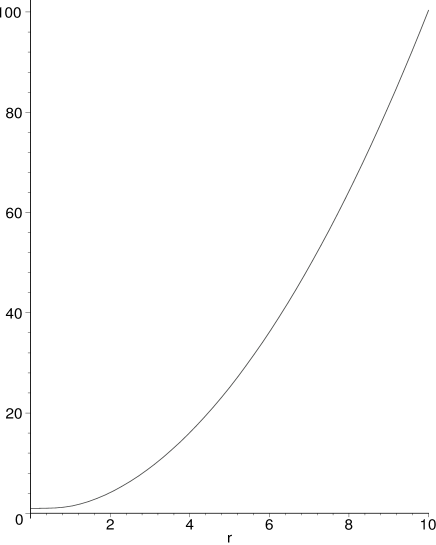
Figure 1: Plot of the energy as a function of $r$, for $s=0$ and taking $C=50$.

Plots of the energy function as a function of $r$ show that at $s=0$ it is monotonically increasing. Figure  1 shows such a plot. This behaviour means that as the D2-brane starts collapsing from rest at some large radius $r_{0}$, there is no smaller radius where the energy can take the same value at $t=0$ while returning to zero velocity. If the potential had a minimum, a conventional bounce would be possible with the radial evolution slowing down to zero velocity and then re-expansion starting with a change in sign of the radial velocity. So clearly such a bounce does not happen with the first $1/N$ correction.

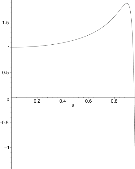
Figure 2: Plot of energy as a function of $s$, for $r=0$ and with $C=50$.

Plots of the energy as a function of $s$ at fixed $r$ show an extremum. Figure  2 shows such a plot at $r=0$. If the energy is bounded above at $r=0$, this means that a D2-brane, starting from zero velocity at sufficiently large $r_{0}$ (hence sufficiently large energy), cannot reach zero radius. This may seem paradoxical given the conclusions to be drawn from the plot above of energy as a function of $r$ at $s=0$. Further insight can however be obtained by plotting contours of constant energy in the $(r,s)$ plane.

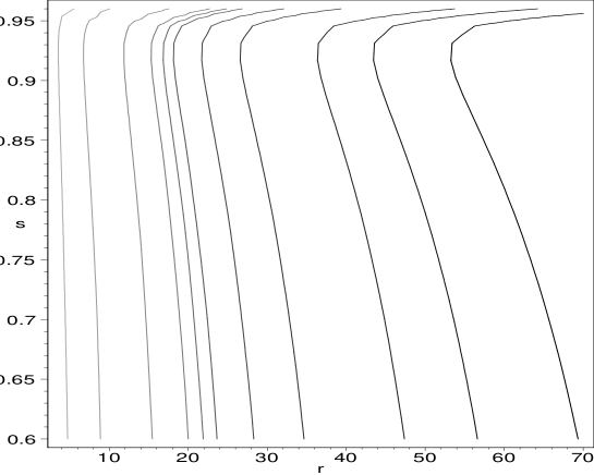
Figure 3: Plot of constant energy contours as a function of $r$ and $s$, with $C=100$. The energy of the contours is increasing from left to right.

Figure 3 shows contour plots of the energy (69) as a function of $r$ and $s$. We have chosen $C=100$ as an example. If we do not include the $1/C$ correction the constant energy contours all reach down to zero radius. The key feature is that ${\partial E\over\partial s}=0$ at a point where $s=s_{m}\neq 0$. This does not happen for ordinary mechanical systems described by energy functions of the form $E={1\over 2}ms^{2}+V(r)$. For such energy functions ${\partial E\over\partial s}=0$ only at the point $s=0$. As we will see from analytic considerations in section 4.2, solutions to ${\partial E\over\partial s}=0$ or equivalently ${\partial E\over\partial\gamma}=0$ do exist for $\gamma\sim C^{1/4}$.

More detailed numerical investigation of the trajectories are possible. For fixed initial energy $E_{0}$ or initial position $r_{0}$ (or equivalently $U_{0}$) where the velocity is zero, we can solve the equation $E(\gamma,U)=E_{0}$ for $U(\gamma,E_{0})$. The equation is quartic and has four solutions, one of which is the physical one. This solution can be followed as $\gamma$ is changed from unity to some large number. For $E_{0}$ corresponding to $U_{0}>1$ but $U_{0}<\sim C^{1/4}$ we find that the classical path describes $U$ decreasing monotonically to $U=1$. These paths, which we may call perturbative paths , are small ${1\over C}$ perturbations of the paths obtained from ${\cal{L}}_{0}$. For larger values of $U_{0}$, the path encounters a minimum radius at some finite value $\gamma_{m}$ and proceeds to increasing $U$, which in fact approaches infinity at a finite upper bound.

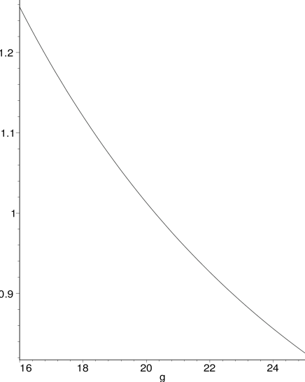
Figure 4: Plot of $U$ as a function of $\gamma=g$ along a solution, with $C=50^{4}$ and $E_{0}=20$

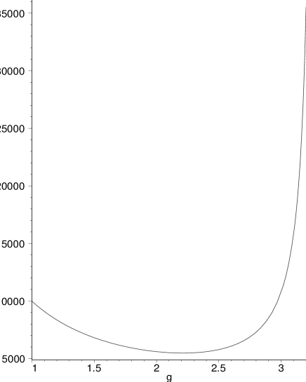
Figure 5: Plot of $U$ as a function of $\gamma=g$ along a solution, with $C=50$ and $E_{0}=100^{2}$

Figure 4 shows the classical path in the $(U,\gamma)$ plane for $C=50^{4}$ and $E_{0}=20$. For these choices, $U$ decreases continuously through $U=1$ or $r=0$. Figure 5 shows the classical path in the $(U,\gamma)$ plane for $C=50^{4}$ and $E_{0}=100^{2}$. For these choices, $U$ decreases until it reaches a minimum and then increases apparently to infinity at a finite value of $\gamma$. Beyond this limiting $\gamma$ the quartic equation for $U$ given by $E(\gamma,U)=E_{0}$ has no physical solution. Along these paths we can also compute an effective mass $\sqrt{E^{2}-p^{2}}$ and the (proper) acceleration. We will discuss these further in Section 8.

4.2 Extrema

The extrema in the energy contour are one of the novel features of ${\cal{L}}_{1}$. As we will elaborate on later, they occur in a region where the $1/N$ expansion is becoming problematic, but we will nevertheless study them in more detail since it is entirely possible that such extrema occur in the finite $N$ case.

On a contour of constant energy one has $dE=0$. To first order in variations of $\gamma,U$ we can write $dE=({\partial E\over\partial\gamma})_{U}d\gamma+({\partial E\over\partial U})_{\gamma}dU$. At an extremum of position along the energy contour, we have $dU=0$. This means that

$$({\partial E\over\partial\gamma})_{U}=0$$ (70)

at that point. Equivalently we have

$$({\partial U\over\partial\gamma})_{E}={({-{\partial E}\over{\partial\gamma}})_{U}\over({{\partial E}\over\partial U})_{\gamma}}$$ (71)

If we consider $U$ as a function of $\gamma$ along a constant energy contour, an extremum of $U$ requires the vanishing of the energy derivative (70).

This gives us a quadratic equation for $U^{2}$ in terms of $\gamma$

$$U^{4}\Big{(}-1+5{\gamma^{4}\over 2C}-{2\gamma^{2}\over C}\Big{)}+U^{2}\Big{(}{-\gamma^{2}\over C}+{2\over 3C}\Big{)}-{1\over 6C}=0$$ (72)

This is solved by

$$U^{2}={{({\gamma^{2}\over C}-{2\over 3C})\pm\sqrt{({\gamma^{2}\over C}-{2\over 3C})^{2}+{2\over{3C}}(-1+{5\gamma^{4}\over{2C}}-{2\gamma^{2}\over C})}}\over{2(-1+5{\gamma^{4}\over{2C}}-{2\gamma^{2}\over C})}}$$ (73)

For $\gamma$ close to $1$ the denominator is negative, while the argument of the square root is negative as it is dominated by ${-2\over 3C}$ at large $C$, so there is no real solution for $U$. The positive branch must be chosen for a real solution to be possible. For $C$ large compared to $1$, and $\gamma^{2}\sim\sqrt{C}$, the denominator changes sign and there is a real solution. The minimum $\gamma$ which allows an extremum is obtained by setting the denominator to zero. This gives

$$\gamma^{2}={1\over 5}(2+\sqrt{4+10C})\sim\sqrt{2\over 5}\sqrt{C}$$ (74)

where we have used the large $C$ approximation in the last step. The associated minimal velocity is $s^{2}=1-\sqrt{{5\over 2}}{1\over\sqrt{C}}$.

When $\gamma$ is very large compared to $C$, we again have no physical solution, because $U$ becomes close to zero, whereas for real $r$ it must be larger than $1$. The upper bound on $\gamma$ for allowed extrema is obtained by setting $U=1$ in (72) and solving for $\gamma$. This gives

$$\gamma^{2}={1\over 5}(3+\sqrt{4+10C})\sim\sqrt{2C\over 5}$$ (75)

Comparing the above two equations, we see that there is a very thin range of $\gamma$ which allows the extremum to exist.

While there is a finite range of velocities which allows the extremum to exist, there is no bound on $r$. This is a bit surprising since we expect the extremum to occur in a sense near the origin. This can still be true in the following sense. If we start the collapse with zero velocity at some position $U_{0}$, and ask for the minimum $U$ reached, we will get a minimum which is a function of $U_{0}$. Let us denote this minimum as $U_{m}(U_{0})$. We would like to prove that ${U_{m}(U_{0})\over U_{0}}\sim{1\over C^{\alpha}}$ where $\alpha$ is a positive number, so that this approaches zero in the large $C$ limit. Now consider a brane starting with zero velocity. Substitute $\gamma=1$ in (69) to obtain the energy $E_{0}$ at the starting position $U_{0}$

$$E_{0}(U_{0})=U_{0}+{1\over 6CU_{0}^{3}}\Big{(}U_{0}^{2}-1\Big{)}^{2}\$$ (76)

We can determine $\gamma$ as a function of $U$ along the curve of extrema by solving the quadratic equation for $\gamma^{2}$ in (72). This gives

$$\gamma_{m}^{2}={(3+6U_{m}^{2})+\sqrt{24-24U_{m}^{2}+36U_{m}^{4}+90U_{m}^{2}C}\over 15U_{m}^{2}}$$ (77)

Substitute this in the energy formula (69) to get a function $E(U_{m})$ given by

$$E(U_{m})={{2(45+90U_{m}^{2}+15D)^{1\over 2}}(90U_{m}^{4}C+18-48U_{m}^{2}+D+12U_{m}^{4}+2U_{m}^{2}D)\over 3375U^{4}C}$$ (78)

where $D$ is given by

$$D=\sqrt{(24-24U_{m}^{2}+36U_{m}^{4}+90U_{m}^{4}C)}$$ (79)

Equating $E(U_{m})=E(U_{0})$ gives an equation which determines $U_{m}(U_{0})$. This becomes tractable if we use the large $C$ approximation (assuming $U_{m}$ is sufficiently small compared to $C$). We find that $U_{m}/U_{0}=C^{-1/4}f_{0}(U_{0})+C^{-3/4}f_{1}(U_{0})+\cdots$, where $f_{0}(U_{0})\sim 1+{\cal{O}}({1\over U_{0}^{2}})$ and $f_{1}(U_{0})\sim 1+{\cal{O}}({1\over U_{0}^{2}})$.

4.3 Energy-momentum relation

We now turn to dispersion relations. The momentum is

$$p = {1\over\lambda\sqrt{C}}{\partial L\over\partial s}$$ (80)

$$= \gamma Us-{\gamma s\over 6U^{3}C}(3U^{2}\gamma^{2}+1)(U^{2}\gamma^{2}-1)$$

We have included a factor of ${1\over\lambda\sqrt{C}}$ for convenience. Note that the formula for the momentum, like that for the energy, has at the leading term the standard form of special relativity, with $U$ playing the role of mass. We would like to obtain an equation for $E(p)$ which can be interpreted as a deformed dispersion relation.

Let the corrected speed be

$$s={p\over\sqrt{p^{2}+U^{2}}}+{s_{1}\over C}$$ (81)

where we will determine $s_{1}$ as a function of $U$ and $p$. The corrected $\gamma$ variable is

$$\gamma=\Big{(}1+{p^{2}\over U^{2}}\Big{)}^{1/2}-{p\over U}\Big{(}1+{p^{2}\over U^{2}}\Big{)}{s_{1}\over C}$$ (82)

Substituting this in (80) and keeping the leading term in the $1/C$ expansion gives us a linear equation for $s_{1}$. The solution of this is

$$s_{1}={-(p^{2}+U^{2})^{-3/2}\over 6U^{2}}(3U^{2}+3p^{2}+1)(U^{2}+p^{2}-1)p$$ (83)

Substituting in the corrected speed (or the corresponding corrected $\gamma$) in (69) we find the first-order corrected energy formula as a function of $p$ is

$$E = \sqrt{p^{2}+U^{2}}~{}+~{}{(p^{2}+U^{2})^{-3/2}\over 6CU^{4}}(U^{2}+p^{2}-1)(U^{2}-3p^{2}-1)(U^{2}+p^{2})^{2}$$ (84)

$$- {p^{2}\over 6CU^{4}}(3U^{2}+3p^{2}+1)(U^{2}+p^{2}-1)$$

There has been a lot of discussion of deformed dispersion relations recently in the context of inflation (see [24], for example). The deformed dispersion relation we are getting does not have a smooth limit in the zero “mass” limit of $U=0$. In our context this limit is of course unphysical since $U=\sqrt{1+r^{4}}$.

4.4 The time of collapse

It is also possible to determine the time of collapse in this system. The leading formulae for velocity $s$ and the corresponding $\gamma$ are

$$s_{(0)}(U,U_{0})={\sqrt{U_{0}^{2}-U^{2}}\over U_{0}^{2}},\qquad\gamma_{(0)}(U,U_{0})={U_{0}\over U}$$ (85)

We will find the perturbed formulae

$$s=s_{(0)}+{1\over C}s_{(1)}(U,U_{0}),\qquad\gamma=\gamma_{(0)}+{s_{(1)}\over C}\gamma_{(0)}^{3}(1-\gamma_{(0)}^{-2})^{1\over 2}\equiv\gamma_{(0)}+{\gamma_{(1)}\over C}$$ (86)

where the last line defines $\gamma_{(1)}$. We substitute (76) into the left-hand side of (69), and on the right-hand side put in the $1/C$ expansion of the velocity, keeping only the leading terms. This gives

$$E_{0}(U_{0})-U_{0}={\gamma_{(1)}U\over C}+{1\over C}f(\gamma_{(0)},U)$$ (87)

where $f$ is the correction term that appears in (69). This allows us to solve for $\gamma_{(1)}$, or equivalently $s_{(1)}$. We find

$$s_{(1)}={(U_{0}^{2}-1)\over 6U_{0}^{5}}{\sqrt{(U_{0}^{2}-U^{2})}\over U^{2}}(3U_{0}^{4}-U_{0}^{2}U^{2}+U_{0}^{2}+U^{2})$$ (88)

Thus the $1/C$ corrected formula for the speed is

$${dr\over dt}={\sqrt{(U_{0}^{2}-U^{2})}\over U_{0}}+{1\over C}{(U_{0}^{2}-1)\over 6U_{0}^{5}}{\sqrt{(U_{0}^{2}-U^{2})}\over U^{2}}(3U_{0}^{4}+U_{0}^{2}+U^{2}(1-U_{0}^{2}))$$ (89)

and the time of collapse is

$$\int dt = \int dr{U_{0}\over\sqrt{U_{0}^{2}-U^{2}}}-{1\over 6C}\int dr{(U_{0}^{2}-1)(3U_{0}^{2}+1)\over U_{0}U^{2}\sqrt{U_{0}^{2}-U^{2}}}$$ (90)

$$+{1\over 6C}\int dr{(U_{0}^{2}-1)^{2}\over U_{0}^{3}\sqrt{U_{0}^{2}-U^{2}}}$$

These integrals can be evaluated in terms of elliptic functions.

5 Solution in the neighborhood of the extremum

In this section, we will study the behaviour of the brane in the region of the radial extremum found above. Generally, consider the expansion of the energy around the extremum, keeping the second order terms. Consider a constant energy contour parameterised by $\lambda$, i.e we think of coordinates $(G(\lambda),V(\lambda))$, where $G$ is some function of the $\dot{r}$, for example $\gamma$ or $\dot{r}$. $V$ is some function of $r$, for example $U$ or more simply $r$. By expanding the energy in a Taylor series we find at lowest two orders

$$d\lambda\Big{(}{\partial E\over\partial V}{dV\over d\lambda}+{\partial E\over\partial G}{dG\over d\lambda}\Big{)}=0$$ (91)

and

$$d\lambda^{2}\Biggl{(}\frac{1}{2}{\partial E\over\partial V}{d^{2}V\over d\lambda^{2}}+\frac{1}{2}{\partial E\over\partial G}{d^{2}G\over d\lambda^{2}}+{1\over 2}{\Big{(}{dV\over d\lambda}\Big{)}^{2}}{\partial^{2}E\over\partial V^{2}}+{1\over 2}\Big{(}{dG\over d\lambda}\Big{)}^{2}{\partial^{2}E\over\partial G^{2}}+{\partial^{2}E\over\partial G\partial V}{dG\over d\lambda}{dV\over d\lambda}\Biggr{)}=0$$ (92)

Specializing to a point where ${dV\over d\lambda}=0$, then from (91) we have ${\partial E\over\partial G}=0$. Then we obtain

$$\frac{1}{2}{\partial E\over\partial V}{d^{2}V\over d\lambda^{2}}+{1\over 2}{\Big{(}{dV\over d\lambda}\Big{)}^{2}}{\partial^{2}E\over\partial V^{2}}+{1\over 2}\Big{(}{dG\over d\lambda}\Big{)}^{2}{\partial^{2}E\over\partial G^{2}}+{\partial^{2}E\over\partial G\partial V}{dG\over d\lambda}{dV\over d\lambda}=0$$ (93)

If we approximate the equation in the neighborhood of the extremum where ${dV\over d\lambda}=0$ by setting this first derivative to zero we get

$${d^{2}V\over d\lambda^{2}}=-{{\partial^{2}E\over\partial G^{2}}({dG\over d\lambda})^{2}\over{{\partial E\over\partial V}}}$$ (94)

The complete equation derived at order $d\lambda^{2}$ is really (93) but we may hope that some qualitative properties such as the existence of two branches corresponding to reflection with increasing speed or reflection with decreasing speed can be captured by the simpler equation (94). This equation should allow us to prove that the extremum is a minimum of $U$ and that we need a change of branch of the solution at the extremum.

Let us choose $V=r$ , $G=s^{2}\equiv S$ and $\lambda=S$ so that (94) becomes

$${d^{2}r\over dS^{2}}=-2\alpha$$ (95)

where $\alpha=\frac{1}{2}{\partial^{2}E\over\partial S^{2}}/{\partial E\over\partial r}$ evaluated at the extremum. Equation (95) can be solved in the neighborhood of the minimum to give

$$(r-r_{m})=-\alpha(s^{2}-s_{m}^{2})^{2}$$ (96)

We know that $r>r_{m}$ because plots show that the constant energy contours have a minimum and $\alpha$ is less than zero. We can now write the squared velocity

$$s^{2}=s_{m}^{2}\pm\sqrt{{r_{m}-r\over\alpha}}$$ (97)

Hence

$${dr\over dt}=\pm\sqrt{s_{m}^{2}\pm\sqrt{r_{m}-r\over\alpha}}$$ (98)

which can be solved for the time elapsed

$$\int dt=\pm\int dr{1\over\sqrt{s_{m}^{2}\pm\sqrt{r_{m}-r\over\alpha}}}$$ (99)

When we choose the outer negative sign, $r$ decreases with increasing time, whereas when we choose the outer positive sign, $r$ increases with increasing time. The collapsing solution cannot be continued past $r_{m}$ because the formula for time elapsed would become complex. These two solutions can be patched at $r=r_{m}$. The radial velocity is discontinuous at the patching, but the time evolution described by the patched solutions is consistent with energy conservation.

Note that there is also a choice of sign inside the square root. If we switch the choice of this sign in patching solutions at the extremum, then the collapsing brane re-expands along the second branch, which means that, when it reaches the original starting position (where it had zero velocity), it is travelling close to the speed of light. If we do not make this switch of sign inside the square root upon patching, the brane re-expands along the same branch as it was collapsing and reaches zero velocity at the starting position.

If we use the form $(V,G)=(s,r)$ and use $\lambda=s$, the differential equation (94) becomes

$${d^{2}r\over ds^{2}}=-2\beta$$ (100)

where $\beta=\frac{1}{2}{\partial^{2}E\over\partial s^{2}}/{\partial E\over\partial r}$. Then

$$\int dt=\int dr{1\over{s_{m}\pm{\sqrt{r-r_{m}}\over\beta}}}$$ (101)

Here the overall choice of sign visible in (99) is not apparent. However we know by the time reversal invariance of the Lagrangian that solutions which have an extra $\pm$ in front of the integral are also allowed. This time reversal invariance was kept manifest when we worked with the variables $(r,s^{2})$.

A more precise treatment of the local differential equation in the neighbourhood of the extremum continues to reveal that $s-s_{m}$ is double valued there. With the choice $(G,V)=(s,r)$, $\lambda=s$, if we keep terms involving the first derivative we get an equation of the form

$$a{\partial^{2}r\over\partial s^{2}}+b\Big{(}{\partial r\over\partial s}\Big{)}^{2}+c{\partial r\over\partial s}+d=0$$ (102)

where the constants are given by

$$a={E_{r}^{(m)}\over 2},~{}~{}~{}~{}b={E_{rr}^{(m)}\over 2},~{}~{}~{}~{}c=E^{(m)}_{rs},~{}~{}~{}~{}~{}d={E^{(m)}_{ss}\over 2}$$ (103)

Equation (102) is the Riccati equation with constant coefficients. We can solve this as follows. Use variables ${y={dr\over ds}}$ to rewrite (102) as

$$a{dy\over ds}+by^{2}+cy+d=0$$ (104)

The roots of the quadratic polynomial in $y$ play an important role in the solutions. These roots are

$$a_{+}={-c+D\over 2b},\qquad a_{-}={-c-D\over 2b}$$ (105)

where we defined $D=\sqrt{c^{2}-4db}$. Numerical check shows that $D$ is real. Integrating once gives

$$\int ds=-{a\over b}{1\over(a_{+}-a_{-})}\ln\left({y-a_{+}\over y-a_{-}}\right)$$ (106)

Imposing the condition that $y={dr\over ds}=0$ at $s=s_{m}$ fixes the integration constant to give

$$(s-s_{m})=\frac{a}{D}~{}~{}\left(~{}\ln~{}\Big{(}{a_{+}\over a_{-}}\Big{)}-~{}\ln~{}\Big{(}{y-a_{+}\over y-a_{-}}\Big{)}~{}\right)$$ (107)

One more integration and the condition that $r=r_{m}$ at $s=s_{m}$ gives

$$r-r_{m}=a_{+}(s-s_{m}) + {a\over b}~{}\ln\left(~{}1-\frac{a_{+}}{a_{-}}\exp\Big{(}{\frac{b(a_{-}-a_{+})}{a}(s-s_{m})\Big{)}}~{}\right)$$ (108)

$$- \frac{a}{b}~{}\ln\left(~{}1-{a_{+}\over a_{-}}~{}\right)$$

The original differential equation (104) is symmetric under exchange of the roots $a_{\pm}$ and as expected the final solution can be manipulated into the form

$$r-r_{m}=a_{-}(s-s_{m}) + {a\over b}\ln\left(1-\frac{a_{-}}{a_{+}}\exp\bigg{(}{\frac{b(a_{+}-a_{-})}{a}(s-s_{m})\bigg{)}}\right)$$ (109)

$$- \frac{a}{b}~{}\ln\left(~{}1-{a_{-}\over a_{+}}~{}\right)$$

Expanding the right-hand side of (108) or (109) gives

$$(r-r_{m})=-{E_{ss}^{(m)}\over 2E_{r}^{(m)}}\Big{(}s-s_{m}\Big{)}^{2}$$ (110)

in agreement with the approximation which dropped the ${dr\over ds}$ terms in the equation. From (110) it is clear that for a fixed $r$ there are two values of $s$, one above $s_{m}$ and one below.

We can also use the time $t$ as the parameter $\lambda$ and obtain an equation which looks a little more complicated but can nevertheless be solved. It seems that the time variable may be less useful since $dr/dt$ has a discontinuity at the extremum. In any case the equation is now

$$E_{r}^{(m)}\ddot{r}+{1\over 2}E_{rr}^{(m)}(\dot{r})^{2}+{1\over 2}E_{ss}^{(m)}({\ddot{r}})^{2}+E_{rs}^{(m)}\ddot{r}\dot{r}=0$$ (111)

This can again be solved.

5.1 Quantum mechanics near the extremum

Equation (100) can be viewed as describing the evolution of $r$ as a function of a “time” variable $s$. We can write down a Lagrangian which leads to the equation and a corresponding Hamiltonian which generates translations along the $s$ direction

$${d^{2}\psi\over dr^{2}}+br\psi=E\psi$$ (112)

The solutions to this equation are Airy functions. The correct boundary condition is to require that the solutions die off for $r<r_{m}$. This implies oscillatory behaviour with a damped amplitude as the magnitude of $s-s_{m}$ increases. It is important to note that in this quantum mechanical set-up $s<s_{m}$ and $s>s_{m}$ are treated symmetrically.

When the terms ${dr\over ds}$ are kept the system becomes dissipative. Such systems cannot be quantised in an ordinary way, but they can be described quantum mechanically by enlarging the system to include a bath of bosonic oscillators, see for example [25, 26]. ( A connection between string theory and this quantization of dissipative systems has in fact been made in [27] ). The correlation functions $<r(s)r(s^{\prime}>$ can be considered. Such treatments in terms of a bath of oscillators can be viewed as simulating the interaction of the massless degrees of freedom including $r$ with the stringy spectrum of open string modes. It is possible that the extra degrees of freedom required are just the additional modes that live on the brane world-volume, e.g the various fluctuations of the fields (which have been neglected in the solutions where we study purely radial evolution). The important conclusion for our purposes is that whereas the classical evolution is ambiguous at the turning point, a quantum mechanical set-up allows computations of correlators associated with different points along the trajectory on either side of the extremum. This leads us to anticipate that a more complete stringy treatment will allow the formulation of probabilities for the evolution along the two branches.

It may appear that the conclusions from attempting the above quantum mechanical discussion are artefacts of the exotic choice of $s$ as time. However, the ordinary time can also be used to describe the equations, which are then of higher order. This again suggests that we need additional degrees of freedom. In fact it has been argued that particle systems with higher derivative actions share some stringy properties such as the Virasoro algebra [28]. The conclusion from this discussion is again that an attempt to do quantum mechanics leads to the need for extra degrees of freedom, which are indeed expected in this stringy context. While these stringy modes are not relevant for most of the trajectory, at the extremum the only possible classical evolutions involve discontinuities in velocity, hence formally infinite accelerations. Since small accelerations are a requirement for the low energy effective action to be useful, in this case we expect that extra degrees of freedom become relevant.

6 Higher order corrections to the Lagrangian

Based on the results of Section 3, the next order corrections to the Lagrangian of (65) give the result

$${\cal{L}}_{2}=\left(1-{2\over 3}C{\partial^{2}\over\partial C^{2}}+{14\over 45}C^{2}{\partial^{4}\over\partial C^{4}}+{8\over 9}C{\partial^{3}\over\partial C^{3}}\right){\cal{L}}_{0}$$ (113)

The energy function to this order is

$${\cal{E}}_{2} = \gamma U-{\gamma\over 6CU^{3}}(\gamma U+1)(\gamma U-1)(3\gamma^{2}U^{2}+1-4U^{2})$$

$$+ {\gamma\over 120C^{2}U^{7}}(\gamma U-1)(\gamma U+1)\Big{(}245\gamma^{6}U^{6}-640\gamma^{4}U^{6}+105\gamma^{4}U^{4}$$

$$+ 528\gamma^{2}U^{6}-256\gamma^{2}U^{4}+63\gamma^{2}U^{2}-128U^{6}+176U^{4}-128U^{2}+35\Big{)}$$

It is possible to repeat the analysis of Section 4, studying the effects of the above terms of order $1/C^{2}$. We omit the details. In summary, as in the study of the Lagrangian ${\cal{L}}_{1}$, there is a class of perturbative paths in $(\gamma,U)$ space (for $U_{0}<\sim C^{1/4}$), which are similar to the ones arising from the Lagrangian ${\cal{L}}_{0}$. For higher $U_{0}$ the paths still end at $U=1$ without going through the extremum seen with ${\cal{L}}_{1}$, but there are important differences. The proper acceleration does not increase far beyond $1$ and the final $\gamma$ at $U=1$ increases with $U_{0}$ much slower than would be anticipated by extrapolation from the final $\gamma$ for the perturbative paths. This suggests some sort of repulsive force. It also indicates that there may be a class of non-perturbative (in the sense of the $1/N$ expansion) paths having small proper accelerations which allow simple reliable treatment with the low energy effective actions neglecting the higher derivative terms.

Going to one further order, using the term suggested by the expression (62), however restores the extremum when these terms contribute. Thus, as this emphasises, in regimes where higher order terms are not negligible it is necessary to obtain information about the exact structure of $Str(\alpha_{i}\alpha_{i})^{n}$. To this end, in Section 7 we will derive and study the exact expression for this when the spin half representation is used.

7 Exact evaluation of the symmetrised trace for spin half

In this section, the ${{\cal{C}}_{n}}$ operator will be evaluated exactly for the spin $1/2$ case. We will be using some of the notation and techniques from Section (3.1). Consider patterns of the form

$$\alpha_{3}^{2n-i_{2k}}\alpha_{+}\alpha_{3}^{i_{2k}-i_{2k-1}-1}\cdots\alpha_{3}^{i_{3}-i_{2}-1}\alpha_{+}\alpha_{3}^{i_{2}-i_{1}-1}\alpha_{-}\alpha_{3}^{i_{1}-1}$$ (114)

These are the only patterns that contribute for spin $1/2$ since any pattern containing $(..)\alpha_{-}(..)\alpha_{-}(..)$ (where $(..)$ as in Section 2 stands for arbitrary powers of $\alpha_{3}$) gives zero when acting on the highest weight of the two-dimensional representation. This is an important simplification compared to the case of general $J$. Expressions of the form (114) are to be summed with summation symbol $\sum_{\vec{i}}$ defined as

$$\sum_{i_{2k}=2k}^{2n}\sum_{i_{2k-1}=2k-1}^{i_{2k}-1}\cdots\sum_{i_{2}=2}^{i_{3}-1}\sum_{i_{1}=1}^{i_{2}-1}$$ (115)

After commuting all the $\alpha_{3}$’s to the left we get

$$\sum_{\vec{i}}(\alpha_{3}-2)^{(i_{2}-i_{1}-1)+(i_{4}-i_{3}-1)+\cdots+(i_{2k}-i_{2k-1}-1)}\alpha_{3}^{i_{1}+(i_{2}-i_{1}-1)+\cdots+(i_{2k}-i_{2k-1}-1)}$$

$$\qquad\qquad\qquad\times\,\alpha_{+}\alpha_{-}\alpha_{+}\alpha_{-}\cdots\alpha_{+}\alpha_{-}$$ (116)

Further simplifications are $\alpha_{3}=2J=1$ and $\alpha_{3}-2=(-1)$. As a result the expression in (7) evaluates on the highest weight state to

$$2^{k}\sum_{\vec{i}}\Big{(}-1\Big{)}^{-k+\sum_{p=1}^{2k}i_{p}}$$

We also used $N(1,1)=2$ for $J={1\over 2}$. The sum over $i$ can be simplified by defining variables

$$\hat{i}_{s}=i_{s}-s,\quad s=1,...,2k$$ (117)

With these variables the expression in (7) simplifies to

$$2^{k}\sum_{\hat{i}_{2k}}^{2n-2k}\cdots\sum_{\hat{i}_{2}=0}^{\hat{i}_{3}}\sum_{\hat{i}_{1}=0}^{\hat{i}_{2}}(-1)^{\hat{i}_{1}+\hat{i}_{2}+\cdots\hat{i}_{2k}}={2^{k}n!\over(n-k)!k!}$$

In relating the patterns to the symmetrised trace there is a combinatoric factor (30). Taking that into account along with the above, we have for spin $1/2$ that the symmetrised power of the quadratic Casimir ${{\cal{C}}_{n}}$ is

$${{\cal{C}}_{n}}={(n!)^{2}\over(2n)!}\sum_{k=0}^{n}{2^{2k}(2n-2k)!\over((n-k)!)^{2}}=(2n+1)\equiv f(n)$$ (118)

Now we can calculate the Lagrangian. Let $\hat{C}=\alpha_{i}\alpha_{i}$. Then

$$L = -{\rm Str}\sqrt{1+\hat{C}r^{4}}\sqrt{1-\hat{C}s^{2}}$$ (119)

$$= -{\rm Str}\sum_{l=0}^{\infty}\sum_{m=0}^{\infty}r^{4l}s^{2m}(\hat{C})^{l+m}{1/2\choose l}{1/2\choose m}(-1)^{m}$$

$$= -N\sum_{l=0}^{\infty}\sum_{m=0}^{\infty}r^{4l}s^{2m}f(l+m){1/2\choose l}{1/2\choose m}(-1)^{m}$$

$$= -N\sum_{n=0}^{\infty}\sum_{l=0}^{n}f(n)r^{4l}s^{2n-2l}{1/2\choose l}{1/2\choose n-l}(-1)^{n-l}$$

The factor of $N(=2)$ comes from the trace, and the binomial factors are expressed in terms of Gamma functions as

$${1/2\choose l}={\Gamma(3/2)\over\Gamma(3/2-l)\Gamma(l+1)}$$ (120)

The energy can be computed to be

$$E(r,s) = -N\sum_{l=0}^{\infty}\sum_{m=0}^{\infty}f(l+m)(2m-1){1/2\choose l}{1/2\choose n-l}(-1)^{m}r^{4l}s^{2m}$$

$$= -N\sum_{n=0}^{\infty}\sum_{l=0}^{n}f(n)(2n-2l-1){1/2\choose l}{1/2\choose n-l}(-1)^{n-l}r^{4l}s^{2n-2l}$$

If we sum over powers of $r$ first and then over powers of $s$ we get

$$E(r,s)=2{(1+2r^{4})\over\sqrt{(1+r^{4})}}{}_{2}F_{1}({1\over 2},{3+4r^{4}\over 2+2r^{4}};{(1+2r^{4})\over(2+2r^{4})},s^{2})$$ (122)

If we sum over powers of $s$ first and then over powers of $r$ we get

$$E(r,s)=2{1\over(1-s^{2})^{3/2}}{}_{2}F_{1}({2s^{2}-3\over 2s^{2}-2},{-1\over 2};{-1\over 2s^{2}-2},-r^{4})$$ (123)

These are both useful expressions.

It is useful to recall the following facts about the hypergeometric function ${}_{2}F_{1}(z)$. This function has branch points at $z=1$ and $z=\infty$, and there is a branch cut extending from $1$ to $\infty$. Formulae are available for the discontinuity across the branch cut. In (122) attempting to continue past $s=1$ runs into the branch cut. Continuation past $s=1$ to $s>1$ requires specification of the sheet. Physically we are not interested in these super-luminal speeds in any case. In (123) the hypergeometric function can be continued past $r=1$ to large positive $r$ even though the the original sum over powers of $r$ diverges for $r>1$.

It is instructive to specialize (122) or (123) to the case of $r=0$ or $s=0$.

$$E(r=0,s) = 2{1\over(1-s^{2})^{3/2}}$$ (124)

$$E(r,s=0) = 2{(1+2r^{4})\over\sqrt{1+r^{4}}}$$ (125)

From (125) we see that the energy grows monotonically with $r$. This means there is no smooth bounce. From (124) there is no extremum as a function of $s$ at $r=0$. Hence there is no exotic bounce at $r=0$. Further numerical investigation shows that there is no such extremum when $r>0$. Hence the exotic bounces of the kind studied in section 4 with the first $1/N$ correction, do not occur for spin $1/2$. Whether such extrema occur for other finite values of $N$ is an interesting open question.

The appearance of the limiting velocity $s=1$ in (122) – (124) shows that the symmetrised trace prescription correctly captures the expected relativistic barrier. This does not seem evident from the original form of Lagrangians such as (1).

8 Regimes of validity

Neglecting higher spatial derivatives implies that the D2-brane picture only works for distances larger than the string scale, or $r>1$ in dimensionless units. We also need to consider higher orders in time derivatives.

We first discuss issues of regimes which are related to radial velocities and their comparison to $C$, before considering accelerations. For the original unperturbed solution, described in Section 2, $E=\sqrt{(1+r^{4})\over(1-\dot{r}^{2})}$ and if $r_{0}$ is the initial position where $\dot{r}=0$, then $\dot{r}^{2}={r_{0}^{4}-r^{4}\over 1+r_{0}^{4}}$. The subsequent analysis of $1/N$ corrections has shown that higher orders in the $1/N$ expansion are important when $\gamma^{2}\sim\sqrt{C}\sim N$. This gives a lower bound on $r$ for the large $N$ zero-brane description to remain valid -

$$r^{4}>{r_{0}^{4}\over N}-1$$ (126)

This lower bound can be much less than $1$, so we can follow the evolution for distances much shorter than the string scale. However it appears that we can follow it all the way to zero if $r_{0}^{4}$ scales like a power of $N$ which is smaller than one.

Indeed, for such choices of $r_{0}$, the paths which solve the equations of motion coming from ${\cal{L}}_{1}$ and ${\cal{L}}_{2}$ have a similar behaviour to the leading order paths. They describe 2-branes collapsing to zero size with maximal proper accelerations which grow as $r_{0}$ grows. The maximal speed reached at zero radius is very close to the speed of light, with $\gamma\sim r_{0}^{2}$. However when $r_{0}$ is larger than $\sim N^{1/4}$, the paths described show qualitative changes. Whether we work with ${\cal{L}}_{1}$ or ${\cal{L}}_{2}$, we find that there is an upper bound on $\gamma$ which is much less than $r_{0}^{2}$.

8.1 Proper Acceleration and effective mass

Two useful quantities to study are the proper acceleration and the effective squared mass. The proper acceleration $\alpha$ is given by $\alpha^{2}={d^{2}x_{\mu}\over d\tau^{2}}{d^{2}x^{\mu}\over d\tau^{2}}$. Useful expressions for $\alpha$ are

$$\alpha=\gamma^{3}{d^{2}r\over dt^{2}}=\gamma^{3}s{ds\over dr}=-\gamma^{3}s\frac{E_{r}}{E_{s}}=-\frac{E_{r}}{E_{\gamma}}$$ (127)

This is the relativistically invariant acceleration and should be expected to control higher derivative corrections to the Born-Infeld action. For recent discussion on the geometry of corrections to brane actions see [30, 31]. An effective mass can be defined by $m^{2}=E^{2}-p^{2}$. For the leading order solution one has $m=\sqrt{1+r^{4}}$. With this effective mass, the formulae for the energy and momentum look like the standard ones of special relativity.

For the leading large $N$ solution

$$\alpha=-2r^{3}{(1+r_{0}^{4})^{(1/2)}\over(1+r^{4})^{(3/2)}}$$ (128)

This shows that the proper acceleration starts at a small value $\alpha\sim{1\over r_{0}}$ at the initial position $r_{0}$, which is taken to be much larger than $1$. It grows to order $1$ at $r\sim r_{0}^{2/3}$ and reaches a maximum of $\alpha\sim r_{0}^{2}$ when $r=1$. It drops back to order $1$ at $r\sim r_{0}^{-2/3}$ and finally to zero when $r=0$. Near the extrema of the phase space curves obtained from ${\cal{L}}_{1}$, where ${ds\over dr}$ is infinite, the acceleration and proper acceleration continuously approach infinity. This suggests that the full stringy degrees of freedom are important, or at least we need some information about the nature of the terms in the effective action involving proper accelerations and higher derivatives.

For the cases of spin half, and the Lagrangian ${\cal{L}}_{2}$, we can study the acceleration numerically. For ${\cal{L}}_{2}$, with $U_{0}<\sim C^{1/4}$, the proper acceleration behaves similarly to that for the solutions to the zeroth order equations of motion coming from ${\cal{L}}_{0}$, reaching large values around $r=1$. Somewhat surprisingly, for very large $U_{0}$, we find that the acceleration remains small (less than $1$ in magnitude) along the trajectory. This is another indication that for such high $U_{0}$ the $1/N$ corrected Lagrangians behave very differently from the leading order ones. The fact that the proper acceleration remains small suggests that there may be interesting time-dependent physics in string theory which is non-perturbative in the $1/N$ expansion but can be reliably described by the Born-Infeld actions, nelecting higher derivative corrections and massive string modes.

For the $1/C$ corrected Lagrangian, ${\cal{L}}_{1}$, we find that there are regions of phase space where the effective mass becomes imaginary. Numerical studies show that as we follow the trajectory of a large $D2$-brane down to small radius in the space parameterised by $(r,s^{2})$, we have a minimum radius and then the curve continues along increasing $s^{2}$ and approaches infinite radius as it asymptotes to a finite upper $s^{2}=s_{E}^{2}<1$. The acceleration and proper acceleration approach zero as $s_{E}$ is approached. The effective mass remains real at the extremum but becomes imaginary near $s_{E}$.

For ${\cal{L}}_{1}$ the effective mass squared is

$$m^{2} \equiv E^{2}-p^{2}=U^{2}\bigl{(}1+{1\over 3C}(\gamma^{2}-U^{-2})^{2}$$ (129)

$$\quad-{1\over 36C^{2}}(\gamma^{2}-U^{-2})^{2}(15\gamma^{4}-16\gamma^{2}+2\gamma^{2}U^{-2}-U^{-4})\bigr{)}$$

The region of interest is at large $U$. Assuming large $U$ and large $\gamma$, the coefficient of $U^{2}$ in the above expression is $1+{\gamma^{4}\over 3C}-{5\gamma^{8}\over 18C^{2}}$. This changes sign at $\gamma^{4}=C/2$. Note that this value of $\gamma$ is larger than the large $C$ location of the extremum $\gamma\sim\sqrt{2C\over 5}$, consistent with the numerical evidence that the extremum is reached before the tachyonic behaviour of the mass squared. For fixed initial conditions, there is also a tachyon appearing with ${\cal{L}}_{2}$ but this also appears at a larger speed than the extremum seen with ${\cal{L}}_{1}$.

As discussed previously, there are two possible classical evolutions after the extremum is reached. One involves bouncing back along the original path, with a discontinuity in velocity. The other is to bounce back along the branch with increasing $s^{2}$. Here we are finding that the first bounce does not encounter the tachyonic region whereas the second does. The immediate neighbourhood of the extremum is free from the tachyon but involves infinite proper accelerations. The correct string description may require string field theory.

Plots of the effective mass as a function of $(r,s)$ continue to show the radial mode becoming tachyonic in certain regions, for ${\cal{L}}_{2}$ as well as for the spin half Lagrangian. Following the classical trajectory of the radius as a function of $\gamma$ for ${\cal{L}}_{2}$, zero radius is reached at finite speed. The effective mass becomes imaginary at some point along the classical trajectory if $U_{0}>\sim C^{1/4}$. The effective squared mass can be plotted as a function of $(r,s)$ for the spin half case. For $r=0$ or small, it becomes tachyonic around $s=0.6$.

A summary of the previous comments is that there is a class of perturbative classical paths which are modified by small $1/C$ corrections. They describe the collpase of branes starting at rest at some $U_{0}$ which corresponds to $\gamma<\sim C^{1/4}$. In the leading Lagrangian ${\cal{L}}_{0}$ the limiting $\gamma\sim C^{1/4}$ are reached for $U_{0}\sim C^{1/4}$. The $1/C$ corrections relevant to such paths can be computed analytically along the lines of Section (4.3) and (4.4). The existence of interesting features such as the extremum we found with ${\cal{L}}_{1}$ requires finite $N$ investigations, which we initiated with the spin half case. If we find such extrema in the finite $N$ case, understanding the complete picture requires information about higher orders in time derivatives, which should be obtained from string theory. This is because the proper acceleration diverges at these extrema. Alternatively we may go beyond the framework of effective actions and study the problem in string field theory. It may also be interesting to explore what happens to such extrema when one considers simple higher derivative Lagrangians which are designed to put an upper limit on the proper acceleration [32].

8.2 The physics of the tachyon

A heuristic argument can be used to predict the existence of the tachyonic effective mass which we found. Imagine an observer sitting at the north pole of the collapsing spherical D2-brane, at $\Phi_{3}=\hat{R}$. In the rest frame of this observer, the north-south axis is Lorentz-contracted, so that the 2-brane looks more like the surface of a pancake. The spherical brane has zero net D2-charge, and can be thought as having positive charge at the north pole and negative charge at the south pole. This follows since the D2-charge density is proportional to $[\Phi_{1},\Phi_{2}]\sim~{}i\Phi_{3}$, which is positive at the north pole and negative at the south pole. Locally then, our observer at the north pole sees themselves at rest on a D2-brane with an anti-D2 brane approaching at high speed. We know that the D2-anti-D2 system has a tachyon when the separation is close to the string scale. The observer also sees a density of magnetic flux which is a distribution of D0-charge, but D0-D2 systems also have a tachyon. It would be interesting to make a more quantitative connection between this picture and the tachyonic effective mass obtained from ${\cal{L}}_{1},{\cal{L}}_{2}$ and the spin half case, in order to understand better this “pancake tachyon”. The insights from [33, 34, 35] which discuss brane-anti-brane systems in the presence of motion and flux may be useful. Another situation where tachyonic behaviour of a radial brane variable has been found recently is described in [36].

It might be argued that the tachyon is an artefact of the symmetrised trace prescription, which is not the correct supersymmetric non-abelian DBI theory. It has been shown that the symmetrised trace prescription must be corrected, based on BPS energy formulas [37, 38, 39]. However, we find it likely that these tachyonic features will survive with these corrections. Indeed it can be argued that ${\cal{L}}_{1}$ is not modified. The form $Str(\alpha\alpha)^{n}=N(C^{n}+a_{1}(n-1)C^{n-1}+n(n-1)(n-2)(an+b)C^{n-2}+\dots)$ follows from general arguments which will hold true even when the symmetrised trace prescription is replaced by something more complicated such as weighting different symmetry patterns with different coefficients. For example, we know that the first correction of the form $C^{(n-1)}$ must vanish for $n=0$ and $1$ because for these values of $n$ we can simply evaluate the traces and check that the leading term $C^{n}$ is accurate. For $n=1$, we have $tr(\alpha_{i}\alpha_{i})=NC$. Assuming that the $n$-dependent coefficients are sufficiently nice functions of $n$, it would follow that the first correction is unchanged by these corrections. The failure of the symmetrised trace prescription starts at $tr(F^{6})$ which translates here into $tr(\alpha_{i}\alpha_{i})^{3}$. Once the structure of the $tr(F^{8})$ terms are known the numbers $a,b$ appearing in the coeffient of $C^{n-2}$ can be determined, and will likely be different from the values $7,-1$ of (23). We have checked that the effective mass to order $1/C^{2}$ can become imaginary at large $\gamma$ for any choice of $a,b$. It is still possible to argue that the tachyon seen in the $1/N$ expansion is really an artefact of the failure of the $1/N$ expansion itself, and that the correct supersymmetric non-abelian Born-Infeld at finite $N$ will not allow such tachyonic behaviour. An important future direction is to develop a proof (which does not look at all obvious) along these lines which disposes of the tachyon, or to develop a more concrete quantitative formulation of the physical nature of the tachyon as outlined above. The expectation that the $1/N$ expansion captures some qualitative features of the finite $N$ physics suggests that the latter avenue will be more fruitful. We have also seen that the symmetrised trace prescription does lead to formulae for the energy which correctly capture the expected relativistic limit $s=1$ in the spin half case.

9 Summary and outlook

A large $N$ approximation to the non-abelian zero-brane action of Myers for time-dependent fuzzy sphere configurations gives equations for the radius which agree with the expected dual picture in terms of a D2-brane with a magnetic flux. These equations have the same form as those for a relativistic particle with a position dependent mass. The $1/N$ corrections to the zero-brane action give rise to modifications of these equations. We studied the energy function for these modified equations in detail.

The simplest solution of interest at large $N$, with Lagrangian ${\cal{L}}_{0}$, describes a D2-brane, with initial radius $R\gg l_{s}$ collapsing to zero radius. Classically this solution can be patched with an expanding solution at zero radius, but the velocity is discontinuous at that point. The zero brane description allows us to deduce that the collapsing radius can be trusted to distances less than the string length. However the speed at very small radius for such a large initial membrane is close to the speed of light. At these speeds, higher orders in the $1/N$ expansion of the zero brane action become important. Another feature to bear in mind is that the proper acceleration becomes large along the classical trajectory. This raises an interesting question of whether the form of the time-dependent solution can be argued to be unchanged throughout the trajectory from large $R$ down to zero, perhaps using arguments along the lines of [40].

Using the first order in $1/N$ corrected Lagrangian ${\cal{L}}_{1}$, we showed that for a large range of initial conditions $R>l_{s}$ ($r>1$ in dimensionless variables), the classical path obtained from ${\cal{L}}_{1}$ is qualitatively similar to that obtained from ${\cal{L}}_{0}$. However for initial conditions which allow $\gamma$ to reach near $C^{1/4}$ along the path, the path described in phase space encounters a minimum at non-zero speed. This conclusion can be reached from the analysis of the energy as a function of $r$ and $s$, where $r$ is the dimensionless radius and $s$ the dimensionless velocity. The contours of constant energy starting from zero velocity at some large radius cannot be continued to zero radius, but rather have a minimum. At the minimum, ${\partial E\over\partial s}=0$, while $s_{min}\neq 0$. Such minima do not occur in simple mechanical systems where $E={m\dot{x}^{2}\over 2}+V(x)$. This occurs in our equations because of the peculiar mixing of the coordinate and velocity in the energy function. At the extremum, the velocity is close to the speed of light. As $N\rightarrow\infty$ this extremum recedes to the relativistic barrier $s=1$, which is why we do not see it in the leading large $N$ approximation. The bounce at the extremum is somewhat peculiar, it involves a discontinuity in the velocity and also an ambiguity in the choice of trajectory after the bounce. These features are made clear by a local analysis of the energy function in the neighbourhood of the singularity. We discussed the quantum mechanical behaviour of the system near this local singularity, and argued that quantum mechanics would provide probabilities for the two trajectories. The discussion is not complete since the equations we are trying to quantise have a non-linear dissipative nature, hinting that the correct quantum treatment requires extra degrees of freedom, such as those that naturally occur in the string set-up when we go beyond the low energy effective action approach and include higher string excitations.

Another consequence of the fact that the velocity at the extremum is close to the speed of light is that the $1/N$ correction term to the Lagrangian is comparable to the leading term for such velocities. This means that the $1/N$ approximation is breaking down in the neighborhood of the extremum. This motivated an analysis of higher orders in the $1/N$ expansion. At the second order in the $1/N$ expansion we found that the extremum disappears, while it reappears again at the third order.

This led us to study the exact Lagrangian for finite $N$. In the case $N=2$, we found that the extremum does not exist, but for general $N$ the existence or otherwise of such extrema is a very interesting open question, which could be addressed using the techniques developed in this paper. If such extrema exist then we will have a new mechanism in string theory for a brane bounce which is intimately related to the non-Abelian structure of D-brane actions.

The technical computations of the $1/N$ corrections require care in dealing with the symmetrised trace. This symmetrised trace leads to the evaluation of certain $SO(3)$ invariants. We presented two approaches to the calculation. One proceeded by evaluating on highest weights. The other used a diagrammatic approach for re-ordering the various terms in the symmetrised product. This latter approach makes interesting connections with knot theory, which may provide a source of new techniques and ideas in this context.

Further computations with ${\cal{L}}_{1}$ included a perturbative computation of the time taken to collapse from an initial radius to some final radius. This perturbative approach is best suited to initial and final radii which are not too far apart. We also computed the energy as a function of momentum giving an interesting deformation of the dispersion relation for a massive relativistic particle, derived directly from the non-Abelian structure of the zero brane action in string theory. Whereas many string-inspired deformations of relativistic dispersion relations have been discussed, this deformation is the first that follows directly from the non-abelian nature of stringy D-brane actions.

In Section 7, we gave a detailed discussion of regimes of validity for the different approximations, taking care to use the proper acceleration rather than the ordinary acceleration as a measure of whether higher derivative corrections are important. Quite generically, we found that the generalised effective mass defined by $\sqrt{E^{2}-p^{2}}$ became tachyonic in certain regions of phase space close to the speed of light. We discussed the physics of this “pancake tachyon” as associated with a geometry which looks very similar to system of brane and anti-brane. We gave arguments against attributing the tachyon to the inadequacy of the symmetrised trace prescription used in the non-abelian Born-Infeld.

Here we have considered the simple situation of a spherical D2-brane collapsing from a dual D0-point of view using the fuzzy 2-sphere construction. It will be interesting to explore similar brane collapse phenomena for higher branes using higher dimensional fuzzy spheres [41, 42, 43, 44, 45, 46, 47]. This may be a new way to explore cosmological bounces in a braneworld context developing works such as [48], with the additional ingredient of the non-abelian Born-Infeld action. Position dependent effective masses have been considered in [49, 50] and earlier references therein. The leading order Lagrangian ${\cal{L}}_{0}$ is a simple example of a relativistic system with position dependent mass. An effective mass can be defined using $m^{2}=E^{2}-p^{2}$ for the higher order Lagrangians. We found tachyonic behaviour in certain regions of phase space close to the speed of light. This problem of the collapsing brane may also have similarities with gravitational collapse of thin shells [51]. Another direction is to look for a gravitational background which corresponds to the time-dependent system of large $N$ zero branes, and find a spacetime interpretation for some of the features we have found such as the bounces and the tachyonic effective masses.

Acknowledgements: We thank David Berman, Clifford Johnson, Costis Papageorgakis, Radu Tatar, Gabriele Travaglini and Angel Uranga for discussions, and José Figueroa-O’Farrill for the use of his files for drawing chord diagrams. Thanks to Simon McNamara and Costis Papageorgakis for pointing out a missing combinatoric factor in equation (118).

References

- [1] A. Sen, Rolling Tachyons, J. High Energy Physics 0204 (2002) 048, hep-th/0203211.
- [2] M. Gutperle and A. Strominger, Spacelike branes, J. High Energy Physics 0204 (2002) 018, hep-th/0202210.
- [3] A. Sen, Rolling Tachyon Boundary States, Conserved Charges and Two Dimensional String Theory, hep-th/0402157.
- [4] L. Cornalba and M.S. Costa, A New Cosmological Scenario in String Theory, Phys. Rev. D66 (2002) 066001, hep-th/0203031.
- [5] H. Liu, G. Moore and N. Seiberg, Strings in Time-Dependent Orbifolds, J. High Energy Physics 0210 (2002) 031, hep-th/0206182.
- [6] G. Horowitz and J. Polchinski, Instability of Spacelike and Null Orbifold Singularities, Phys. Rev. D66 (2002) 103512, hep-th/0206228.
- [7] B. Durin and B. Pioline, Open strings in relativistic ion traps, J. High Energy Physics 0305 (2003) 035, hep-th/0302159.
- [8] P. Townsend, D-branes from M-branes, Phys. Lett. B373 (1996) 68-75, hep-th/9512062.
- [9] M. Douglas, Branes within branes, hep-th/9512077.
- [10] T. Banks, W. Fischler, S. Shenker and S. Susskind, M Theory As A Matrix Model: A Conjecture, Phys. Rev. D55 (1997) 5112-5128, hep-th/9610043.
- [11] D. Kabat and W. Taylor, Spherical membranes in Matrix theory, Adv. Theor. Math. Phys. 2 (1998) 181-206, hep-th/9711078.
- [12] B. Janssen and Y. Lozano, A Microscopical Description of Giant Gravitons, Nucl. Phys. B658 (2003) 281-299, hep-th/0207199.
- [13] C.G. Callan and J.M. Maldacena, Brane Dynamics From the Born-Infeld Action, Nucl. Phys. B513 (1998) 198-212, hep-th/9708147.
- [14] G.W. Gibbons, Born-Infeld particles and Dirichlet p-branes, Nucl. Phys. B514 (1998) 603-639, hep-th/9709027.
- [15] Yi-Fei Chen, J. X. Lu Dynamical brane creation and annihilation via a background flux, hep-th/0405265
- [16] N. Constable, R. Myers and Ø. Tafjord, The Noncommutative Bion Core, Phys. Rev. D61 (2000) 106009, hep-th/9911136.
- [17] M.R. Douglas, D. Kabat, P. Pouliot and S.H. Shenker D-branes and Short Distances in String Theory, Nucl. Phys. B485 (1997) 85-127, hep-th/9608024.
- [18] A.A. Tseytlin, On the nonabelian generalization of Born-Infeld action in string theory, Nucl. Phys. B501 (1997) 41-52, hep-th/9701125.
- [19] R.C. Myers, Dielectric branes, J. High Energy Physics 9912 (1999) 022, hep-th/9910053.
- [20] P. Collins and R. Tucker, Classical and Quantum mechanics of free relativistic membranes, Nucl. Phys. B112 (1976) 150.
- [21] D. Bar-Natan, On the Vassiliev knot invariants, Topology 34 (1995), 423-472.
- [22] A. Kricker, B. Spence, and I. Aitchinson, Cabling the Vassiliev invariants, J. Knot Theory and its Ramifications 6 (3) (1997) 327-358, q-alg/9511024.
- [23] S.V. Chmutov and A.N. Varchenko, Remarks on the Vassiliev knot invariants coming from , Topology 36 1 (1997).
- [24] R.H. Brandenberger and J. Martin, On signatures of short distance physics in the cosmic microwave background, Int. J. Mod. Phys. A17 3663 (2002), hep-th/0202142.
- [25] A. O. Calderra and A. J. Leggett, Annals of Phys. 149 , 374 ( 1983 )
-
[26]
U. Weiss, lecture notes on advanced quantum mechanics,
(Lectures 11,12),
http://www.tn.tudelft.nl/tn/Lectures/vmq.htm;
U. Weiss, Quantum Dissipative Systems, (2nd Edition), Series in Modern Condensed Matter Physics, Vol. 10, World Scientific, 1999. - [27] C.G.Callan and L. Thorlacius, Open string theory as dissipative quantum mechanics Nucl.Phys.B329 117,1990
- [28] P.M. Ho, Virasoro Algebra for Particles with Higher Derivative Interactions, Phys. Lett. B558 (2003) 238-244, hep-th/020818.
- [29] The Wolfram functions site, http://functions.wolfram.com.
- [30] J. deBoer, K. Schalm and J. Wijnhout, General covariance of the non-Abelian DBI-action: Checks and Balances, hep-th/0310150.
- [31] D. Brecher, K. Furuuchi, H. Ling and M. Van Raamsdonk, Generally Covariant Actions for Multiple D-branes, hep-th/0403289.
- [32] V.V. Nesterenko, A. Feoli, G. Lambiase and G. Scarpetta, Regularizing Property of the Maximal Acceleration Principle in Quantum Field Theory, Phys. Rev. D60 (1999) 065001, hep-th/9812130.
- [33] D.S. Bak and A. Karch, Supersymmetric brane-antibrane configurations, Nucl. Phys. B626 (2002) 165 arXiv:hep-th/0110039.
- [34] C. Bachas and C. Hull, Null brane intersections, JHEP 0212 (2002) 035 arXiv:hep-th/0210269.
- [35] R.C. Myers and D.J. Winters, From D-anti-D pairs to branes in motion, JHEP 0212 (2002) 061 arXiv:hep-th/0211042
- [36] D. Kutasov, D-Brane Dynamics Near NS5-Branes, hep-th/0405058.
- [37] A. Hashimoto and W. Taylor IV, Fluctuation Spectra of Tilted and Intersecting D-branes from the Born-Infeld Action, Nucl. Phys. B503 (1997) 193-219, hep-th/9703217.
- [38] A. Sevrin, J. Troost and W. Troost, The non-abelian Born-Infeld action at order , Nucl. Phys. B603 (2001) 389-412, hep-th/0101192.
- [39] A. Sevrin and A. Wijns, Higher order terms in the non-abelian D-brane effective action and magnetic background fields, J. High Energy Physics 0308 (2003) 059, hep-th/0306260.
- [40] L. Thorlacius, Born-Infeld String as a Boundary Conformal Field Theory, Phys. Rev. Lett. 80 (1998) 1588-1590, hep-th/9710181.
- [41] H. Grosse, C. Klimcik and P. Presnajder, On finite 4-D quantum field theory in noncommutative geometry, Commun. Math. Phys. 180 (1996) 429-438, hep-th/9602115.
- [42] J. Castelino, S. Lee and W. Taylor IV, Longitudinal 5-branes as 4-spheres in Matrix theory, Nucl. Phys. B526 (1998) 334-350, hep-th/9712105.
- [43] S. Ramgoolam, On spherical harmonics for fuzzy spheres in diverse dimensions, Nucl. Phys. B610 (2001) 461-488, hep-th/0105006.
- [44] P.M. Ho and S. Ramgoolam, Higher Dimensional Geometries from Matrix Brane Constructions, Nucl. Phys. B627 (2002) 266-288, hep-th/0111278.
- [45] Y. Kimura, Noncommutative Gauge Theory on Fuzzy Four-Sphere and Matrix Model, Nucl. Phys. B637 (2002) 177-198, hep-th/0204256.
- [46] T. Azuma and M. Bagnoud, Curved-space classical solutions of a massive supermatrix model, Nucl. Phys. B651 (2003) 71-86, hep-th/0209057.
- [47] B.P. Dolan, D. O’Connor and P. Presnajder, Fuzzy Complex Quadrics and Spheres, J. High Energy Physics 0402 (2004) 055, hep-th/0312190.
- [48] C.P. Burgess, F. Quevedo, R. Rabadan, G. Tasinato and I. Zavala, On Bouncing Brane-Worlds, S-branes and Branonium Cosmology, JCAP 0402 (2004) 008, hep-th/0310122.
- [49] C. Quesne and V.M. Tkachuk, Deformed algebras, position-dependent effective masses and curved spaces: An exactly solvable Coulomb problem, J. Phys. A37 (2004) 4267-4281, math-ph/0403047.
- [50] A.d.S. Dutra, M. Hott and C.A.S. Almeida, Remarks on supersymmetry of quantum systems with position-dependent effective masses, Europhys. Lett. 62 (2003) 8-13, hep-th/0306078.
- [51] J. Crisostomo and R. Olea, Hamiltonian Treatment of the Gravitational Collapse of Thin Shells, Phys. Rev. D, to appear, hep-th/0311054.