D3/D7 Brane Inflation and Semilocal Strings

Abstract:

Among the inflationary models based on string theory, the D3/D7 model has the advantage that the flatness of the inflaton potential can be protected even with moduli stabilization. However, the Abrikosov-Nielsen-Olesen BPS cosmic strings produced at the end of original D3/D7 inflation lead to an additional contribution to the CMB anisotropy. To make this contribution consistent with the WMAP results one needs an extremely small gauge coupling in the effective D-term inflation model. Such couplings may be difficult to justify in string theory. Here we develop a generalized version of the D3/D7 brane model, which leads to semilocal strings, instead of the topologically stable ANO cosmic strings. We show that the semilocal strings have unbroken supersymmetry when embedded into supergravity with FI terms. The energy of these strings is independent of their thickness. We confirm the existing arguments that strings of such type disappear soon after their formation and do not pose any cosmological problems, for any value of the gauge coupling. This should simplify the task of constructing fully realistic models of D3/D7 inflation.

1 Introduction

Despite the recent period of intense research activity on inflationary models in string theory, it is still a challenging task to derive a realistic model of inflation consistent with the stabilization of all string moduli. A particularly important problem is to reconcile the original idea of brane inflation [1, 2] with an appropriate mechanism of volume stabilization so as to make it a valid model of string theory. One of the most developed models in this context was suggested in [3] based on the mechanisms of volume stabilization proposed in [4, 5]. Recently a particular class of models in string theory with moduli stabilization was constructed in [6]. A major problem associated with inflationary models in warped compactifications of type IIB string theory has to do with the fact that the inflaton in these models (the position of the D3 brane deep inside the warped throat geometry) is a conformally coupled scalar in the effective four-dimensional near de Sitter geometry. Therefore, the mass of such a scalar, $m^{2}_{\phi}$, is close to $2H^{2}={1\over 6}R$, where $H^{2}$ is the Hubble parameter and $R$ is the curvature of de Sitter space. This does not meet the observational requirement $m^{2}_{\phi}\sim 10^{-2}H^{2}$, as was uncovered in [3], where some possible resolutions of this problem were suggested. Additional attempts to solve this problem in closely related settings were recently proposed in [7]. New ideas for string cosmology based on non-linear Dirac-Born-Infeld brane actions were developed in [8].

On the other hand, it has been found recently [9, 10, 11, 12] that a particular brane inflation model, the D3/D7 model [2], features a shift symmetry for the inflaton field. The inflaton in this model is related to the position of a D3 brane with respect to a D7 brane in a $K3\times{T^{2}\over\mathbb{Z}_{2}}$ compactification of type IIB string theory, where $\mathbb{Z}_{2}$ involves both orbifold as well as orientifold operations, $\mathbb{Z}_{2}=\mathcal{I}_{2}\cdot\Omega\cdot(-1)^{F_{L}}$. The inflaton shift symmetry follows from the special geometry in such models, as described in ref. [13].

The D3/D7 model [2] has an effective description as a hybrid inflation [14], or, more specifically, as a D-term inflation model [15, 16]. The flat direction of the inflaton potential is associated with the shift symmetry, which is preserved after the stabilization of the volume modulus. It is broken spontaneously only at the quantum level. This symmetry protects the small inflaton mass during inflation. This is an important advantage, since in other models of inflation in string theory it is difficult to protect the inflaton field in the early universe from acquiring an unacceptably large mass.

In its original form, however, the D3/D7 model [2] with $U(1)$ gauge symmetry has another problem. At the end of inflation, cosmic strings form, giving a contribution to the primordial density perturbations [17]. Such stringy perturbations do not lead to the multiple peak structure in the spectrum of the CMB anisotropies. The data from WMAP show that the contribution of the cosmic strings to the CMB anisotropy should not exceed a few percent of the standard inflationary perturbations [18, 19]. In a general class of brane inflation models, the production, spectrum and the evolution of cosmic strings were studied in [20, 21, 22, 23, 24, 16].

It is interesting to note that the model [3] of $D3/{\overline{D3}}$ inflation in the highly warped throat has a natural mechanism for suppressing the contribution of the cosmic strings to the CMB anisotropy [3]: The effective tension of the produced strings and, therefore, their contribution to metric perturbations, is exponentially suppressed due to the large warp factor. The production of very light cosmic strings in this model and in its generalizations was recently studied in [25]. Note that in the warped region of the geometry there is an $m^{2}\sim H^{2}$ problem with inflation. On the other hand, large warping is known to relieve the problem with cosmic strings. In the D3/D7 model, by contrast, we do not have the $m^{2}\sim H^{2}$ problem, but we also do not have an automatic solution of the cosmic string problem.

There are many ways to address this problem. One may change the theory in such a way as to make the potential somewhat asymmetric, so that stable strings are not formed [26, 27]. Alternatively, one can consider models with extremely small coupling constants, which suppresses the stringy contribution [28, 17, 29]. In particular it was shown in [17] that if one assumes, following [18], that the contribution of cosmic strings to the amplitude of metric perturbations should be smaller than $O(10^{-2})$ of the inflationary contribution, then the effective $g^{2}$ must be smaller than $10^{-10}$. Meanwhile if one follows recent work [19] and assumes that the stringy contribution should not exceed $O(10^{-1})$ of the inflationary contribution, then the constraint on $g^{2}$ which can be obtained following Ref. [17] becomes somewhat less stringent, but it still remains quite strong:   $g^{2}\mathrel{\hbox{\hbox to0.0pt{\hbox{\lower 4.0pt\hbox{$\sim$}}\hss}\hbox{$<$}}}10^{-7}$. In the context of the D3/D7 model with volume stabilization, one expects that the effective $g^{2}$ comes from the D3 brane gauge coupling. It may then be rather difficult to get $g^{2}\mathrel{\hbox{\hbox to0.0pt{\hbox{\lower 4.0pt\hbox{$\sim$}}\hss}\hbox{$<$}}}10^{-7}$ in this context.

A simple and elegant method for solving the cosmic string problem in D-term inflation models has recently been proposed in [30] and [16]. If one simply replicates the charged matter multiplets responsible for the string formation so as to obtain a non-trivial global symmetry such as $SU(2)$, one can render the vacuum manifold simply connected, and the relevant cosmic strings become so-called semilocal strings [31]-[36]. The stability properties of semilocal strings cannot be inferred from topological considerations alone, but also depend on the values of the couplings in the underlying Lagrangian [31]-[35]. Numerical simulations of their evolution suggest, that they do not pose any cosmological problems [37]. As an alternative way to circumvent the cosmic string problem, it was suggested in [16] to embed the D-term inflation model into some model with larger gauge symmetry so that the strings would not be topologically stable.

Following these lines, we will, in this paper, generalize the original version of the $D3/D7$ inflationary model [2] in such a way as to include a larger set of global and/or local symmetries. In order to do so, we first go back to the original model [2] and discuss the precise relation between the brane construction and the associated four dimensional ${\cal N}=2$ supersymmetric gauge theory. In this discussion, we will also carefully take into account the volume modulus dependence at each step so as to update the model with regard to the more recent work on stabilization. The purpose of revisiting the original model [2] is to show how exactly the surviving interacting $U(1)$ gauge group of the effective D-term inflation model is related to the two $U(1)$’s from the D3 and D7 worldvolume theories. This will give us a much better understanding of the original model and will allow us to proceed with generalized models with higher symmetries resulting from brane systems with multiple branes. Furthermore, when we embed this discussion into the compact model of [2] but now with stacks of coincident D3 or D7 branes, we will show that the underlying F-theory picture correctly predicts the local and global symmetries one expects for the cosmology of the model.

Fluxes and non-perturbative effects, providing stabilization of moduli in string theory [38, 4], as well as embedding of the relevant 4-dimensional gauge theory with FI term into 4-dimensional supergravity [28], break ${\cal N}=2$ supersymmetry to ${\cal N}=1$ supersymmetry. The embedding of the standard Abrikosov-Nielsen-Olesen (ANO) cosmic strings into ${\cal N}=1$ supergravity with FI terms have been studied recently in [23]. They were shown to saturate the BPS bound and to preserve one half of the original $\mathcal{N}=1$ local supersymmetry [23]. Their possible relation to D1 strings and wrapped D3 branes in string theory was discussed in [23, 24, 16].

As we show in this paper, the semilocal strings relevant for our generalized D3/D7 inflationary model with global symmetries can likewise be realized as 1/2-BPS solutions in $\mathcal{N}=1$ supergravity. More precisely, we show that there are families of 1/2-supersymmetric semilocal string solutions parameterized by an undetermined integration constant that controls the thickness (or the “spreading”) of the flux tube in the string core. These findings are in agreement with earlier results in related non-supersymmetric models [32, 33, 34] and imply that it does not cost any energy for the semilocal strings of our model to change their thickness.

Finally, we will discuss the production and the cosmological evolution of semilocal strings after inflation in our scenario. Unlike the topologically stable ANO strings, which form loops or can be infinitely long, the semilocal strings formed after inflation look like a collection of loops and open string segments of finite length with monopoles at their ends. This fact, together with the possibility of their spreading at no energy cost, may lead to the absence of long semilocal strings, and, as a result, to the absence of the string-related large-scale metric perturbations. Indeed, numerical simulations suggest that semilocal strings disappear soon after their formation [37]. However, these simulations were performed in the context of a slightly different model, without taking into account the cosmological evolution. For a full quantum mechanical investigation of this issue one can use the methods of lattice simulations of symmetry breaking after hybrid inflation [39]. We hope to perform these calculations in a separate publication. In this paper we restrict ourselves to a simple qualitative analysis of the situation. We will argue that the main conclusions of Ref. [37] should be valid for the semilocal strings produced after inflation in the model studied in [30] and in our paper. This suggests that the generalized D3/D7 model developed in our paper does not have any problems with cosmological perturbations produced by strings, and therefore there is no need to require that the coupling constant $g^{2}$ must be very small.

Thus, the purpose of this paper is threefold: i) To develop the generalized D3/D7 brane model including the volume modulus as well as some global symmetries in addition to the local $U(1)$ gauge symmetry; such models will have semilocal cosmic strings instead of ANO strings. ii) To establish the unbroken supersymmetry of these semilocal strings embedded into ${\cal N}=1$ supergravity with FI terms for arbitrary “spread” parameter. iii) To critically analyse and confirm the arguments existing in the literature [30] that the models with semilocal strings have no cosmological problems.

The organization of this paper is as follows: In section 2 we take a single D3 and a single D7 that is wrapped on a $K3$ manifold with non-compact orthogonal directions. We study the precise world volume actions of the branes when the system is kept in a curved background with appropriate fluxes turned on. This analysis will serve as a dictionary between the world volume coordinates and the known P-term action studied earlier in [17]. In section 2 we do not take the back-reactions of branes and fluxes on the geometry into account. This is addressed in section 3 where we also consider a fully compact scenario using the underlying F-theory picture that was developed in [2]. We show that the F-theory curve correctly reproduces the local and the global symmetries for the system when we have multiple D3 and D7 branes. The back-reactions of branes and fluxes are shown to be given by warp factors that are typically of order one when the $K3$ manifold is fixed at a large volume. In section 4 we come to the analysis of semi-local strings in this model with $U(1)$ gauge symmetry and a global $SU(2)$ symmetry. Earlier studies of semi-local strings in the literature did not address the precise connection with local ${\cal N}=1$ supersymmetry. We show that the semi-local strings can arise as 1/2 BPS solitons in the extended Abelian Higgs model embedded in ${\cal N}=1$ supergravity. Finally in section 5 we discuss the cosmology of the model. We discuss the issue of formation of semi-local strings and their effect on the large scale density perturbations of the universe. We argue that these strings do not cause any problems with cosmological perturbations at any coupling. Therefore, we are not restricted to keep the coupling constant $g^{2}$ very small. This may help to construct fully realistic models of D3/D7 inflation.

2 The $D3/D7$ model, P-term model and the volume modulus

In the first version of the $D3/D7$ model of inflation [2] the internal manifold was assumed to be compact, but the mechanism of stabilization of the volume modulus was not discussed. However, later in [10, 9, 12] the volume modulus and its stabilization in the “inflaton trench” were included into the effective D-term inflation model. Here we will study the dependence on the volume modulus in the $D3/D7$ brane system by carefully keeping track of the powers of the volume, and we will also clarify the origin of the effective 4-dimensional model. Postponing the discussion of six compact dimensions to section 3, we will first consider putting the $D3/D7$ system on a compact K3 with the $D7$ wrapped on the K3. We will also give an explicit map between the usual D-brane variables and the variables used in cosmology from $d=4$ supergravity as in [17].

The basic features of the D3/D7 inflationary model [2] can be easily understood from the general properties of $Dp/D(p+4)$ brane systems (see e.g. [40]). As worked out in [40] for the special case $p=5$, $5-9$ strings have charge $+1$ with respect to the $U(1)$ gauge field on the 9-brane and charge $-1$ with respect to the $U(1)$ gauge field on the 5-brane, whereas for $9-5$ strings the signs are reversed due to their opposite orientation. Two T-dualities then yield the system with $p=3$ which we are interested in. We thus have a D3/D7 system with $3-7$ and $7-3$ strings stretched between the D3 and D7 branes with completely analogous charge assignments.

In the case when the fluxes of the D7 gauge field in the directions orthogonal to the D3 brane are self-dual, the masses of the $3-7$ and $7-3$ strings depend only on the distance between the D3 and D7 branes, and the system has $\mathcal{N}=2$ unbroken supersymmetry. In the case when the D7 fluxes are not self-dual, supersymmetry is spontaneously broken and the masses of the stretched strings have an additional contribution proportional to the amount by which the worldvolume fluxes are not self dual ($(\theta_{1}-\theta_{2})^{2}$ in the notation of [2]). The sign of this contribution depends on the charges of the strings: one string gets a negative contribution and the other one gets a positive contribution, in addition to the positive mass coming from the distance between branes. As a result, the positively charged string may become tachyonic at the critical point where the distance between the branes precisely cancels the contribution due to the non-self-dual flux on the D7 brane. This allows one to identify the D3/D7 brane system with the $\mathcal{N}=2$ version [28, 17] of the gauge theory of the D-term inflation model [15], with one hypermultiplet [2] and a Fayet-Iliopoulos (FI) term.

The splitting of mass in the hypermultiplet leads to the logarithmic correction to the gauge theory potential, which can also be reproduced by the calculation of the one-loop amplitude for the effective interaction between the branes. This field theory one-loop correction will have an additional factor in case that one has more than one hypermultiplet.

The end of the waterfall stage of standard D-term hybrid inflation [14] solves the D-flatness condition, and one ends up with an unbroken supersymmetry and a spontaneously broken $U(1)$ gauge symmetry. In the D3/D7 brane system, this final state corresponds to a bound state, in which the D3 brane is dissolved as a deformed Abelian instanton on the $U(1)$ DBI theory on the D7-brane such that the Chern-Simons coupling on the D7 brane is

$$S_{CS}={1\over 16\pi^{2}}\int_{D7}C_{4}\wedge{\cal F}\wedge{\cal F}=\int_{D3}C_{4}.$$ (2.1)

Here, ${\cal F}_{mn}=(dA-B)_{mn}$ has a contribution from both the D7 worldvolume gauge field and the background NSNS two-form (in the directions orthogonal to the D3). The NSNS two-form plays the role of a noncommutative deformation parameter in this context. The anti-self-dual part of the deformation parameter is related to the constant part of $({\cal F}-\ast{\cal F})$ on the D7-brane. Only when the deformation parameter is non-vanishing does the Abelian instanton solution have finite energy [41]. The D3/D7 bound state has an unbroken supersymmetry, derived from $\kappa$-symmetry on the D7-brane. The endpoint vacuum is therefore described by a non-marginal bound state of D3 and D7-branes that corresponds to the Higgs phase of the gauge theory of the D3/D7 system with the FI term provided by the nonvanishing $\theta_{1}-\theta_{2}$.

The low energy effective action (i.e. to leading order in $g_{s}$ and $\alpha^{\prime}$) for a single D3 brane and a single D7 brane in flat space is

$$S = \int d^{8}x\left[-\frac{1}{4g_{7}^{2}}F_{ST}F^{ST}-\frac{1}{2g_{7}^{2}(2\pi\alpha^{\prime})^{2}}\left((\partial_{\mu}X^{i})^{2}+(\partial_{m}X^{i})^{2}\right)\right]$$ (2.2)

$$+\int d^{4}x\left[-\frac{1}{4g_{3}^{2}}F^{\prime}_{\mu\nu}F^{\prime\mu\nu}-\frac{1}{2g_{3}^{2}(2\pi\alpha^{\prime})^{2}}\left((\partial_{\mu}X^{\prime i})^{2}+(\partial_{\mu}Y^{\prime m})^{2}\right)\right]$$

$$+\int d^{4}x\left[-|D_{\mu}\chi|^{2}-\left(\frac{X^{i}-X^{\prime i}}{2\pi\alpha^{\prime}}\right)^{2}|\chi|^{2}-\frac{g_{3}^{2}}{2}(\chi^{\dagger}\sigma^{A}\chi)^{2}\right]+S_{CS}\quad.$$

The indices are as follows: $\mu$ runs from 0 through 3; $i$ denotes directions 4 and 5; $m$ extends from 6 to 9; and $S,T$ will include both the $\mu$ and $m$ directions. The primed (unprimed) fields are the light open string degrees of freedom on the 3-brane (7-brane). The $\chi$ doublet arises as the lightest degree of freedom from stretched strings between the D3-brane and the parallel D7-brane. That $\chi$ is generically heavy is indicated by its mass which is proportional to $(X^{i}-X^{\prime i})^{2}$. The covariant derivative is $D_{\mu}\chi=(\partial_{\mu}+iA_{\mu}-iA^{\prime}_{\mu})\chi$. Note that $\chi$ has units $L^{-1}$ appropriate for a scalar in four dimensions. Note also that the fields $X^{i}$ have units of $L$, and $A_{\mu}$ has units of $L^{-1}$ in all dimensions. Recall that $g_{p}^{2}=(2\pi)^{p-2}g_{s}\alpha^{\prime(p-3)/2}$. The last term contains the various Chern-Simons terms on the two branes.

We would like to place this system in a background that has some $B_{mn}$ field, a Ramond-Ramond $F_{5}=dC_{(4)}$ turned on (consistent with the underlying orbifold as well as orientifold operation) and has the curved metric

$$ds^{2}=R^{-6}(x)g^{E}_{\mu\nu}dx^{\mu}dx^{\nu}+R^{2}(x)(ds^{2}_{\mathbb{R}^{2}/\mathbb{Z}_{2}}+ds^{2}_{K3})\quad.$$ (2.3)

Here, $g^{E}_{\mu\nu}(x)$ is the four-dimensional metric in the Einstein frame. The function $R(x)$ is a function of the noncompact directions $x^{\mu}$ and is to represent the overall length scale of the compact $K3$. The powers of $R(x)$ in each part of the metric are chosen so that the four dimensional gravitational action is in Einstein frame [5]. The function $R(x)$ should be thought of as a very weak function of $x$ (we will drop its derivatives) which we would aim to stabilize by wrapping branes on some cycles in the fully compact $K3\times T^{2}/\mathbb{Z}_{2}$, invoking the mechanisms of [4].

2.1 The D7 action

First, we will consider the D7 part of the action. In the curved background (2.3), the first line of (2.2) modifies to

$$S_{D7} = \int d^{4}xd^{4}y\sqrt{-g_{E}}R^{-12}\sqrt{g_{K3}}R^{4}\left[-\frac{1}{4g_{7}^{2}}(F_{\mu\nu}F_{\rho\sigma}g_{E}^{\mu\rho}g_{E}^{\nu\sigma}R^{12}+{\cal F}_{mn}{\cal F}_{rs}g_{K3}^{mr}g_{K3}^{ns}R^{-4})\right.$$ (2.4)

$$\left.-\frac{1}{2g_{7}^{2}(2\pi\alpha^{\prime})^{2}}\partial_{\mu}X^{i}\partial_{\nu}X^{j}g_{E}^{\mu\nu}g^{\mathbb{R}^{2}}_{ij}R^{8}\right]+\mu_{7}\frac{(2\pi\alpha^{\prime})^{2}}{2!}\int C_{(4)}\wedge{\cal F}\wedge{\cal F}\ ,$$

where we have neglected the fluctuations of $X_{i}$ in the $K3$ directions and exhibited the powers of $R(x)$ explicitly. The covariant 2-form on the D7 brane consists of 2 parts

$${\cal F}\equiv F-B\equiv dA-B.$$ (2.5)

Here, $F_{mn}$ is the field strength of the vector field $A_{m}$ which lives on the brane and $B_{mn}$ is the pullback of the space-time NSNS two-form field to the worldvolume of the D7 brane. We have also added the relevant Chern-Simons piece induced by the background RR field. Now we take $\int d^{4}y\sqrt{g_{K3}}=V_{K3}$ to be the volume of some fixed $K3$. Carrying out the integral over the $K3$ then yields

$$S_{D7} = \int d^{4}x\sqrt{-g_{E}}\left(-\frac{1}{4\tilde{g}_{3}^{2}}(F_{\mu\nu})^{2}-\frac{R^{-4}}{2\tilde{g}_{3}^{2}(2\pi\alpha^{\prime})^{2}}(\partial_{\mu}X^{i})^{2}\right)$$ (2.6)

$$+\int Vol_{(4)}R^{-12}\left(\frac{-1}{4g_{7}^{2}}\right)\int_{K3}{\cal F}\wedge*{\cal F}+\frac{1}{4\pi g_{s}g_{7}^{2}}\int C_{(4)}\int_{K3}{\cal F}\wedge{\cal F}\quad,$$

where the coupling constants are

$$\frac{V_{K3}R^{4}}{g_{7}^{2}}=T_{7}(2\pi\alpha^{\prime})^{2}V_{K3}R^{4}=\frac{V_{K3}R^{4}}{(2\pi)^{4}\alpha^{\prime 2}}\frac{1}{g_{3}^{2}}=\frac{1}{\tilde{g}_{3}^{2}}\quad.$$ (2.7)

Note that $C_{(4)}$ is part of the background, $not$ from the D3. The ${\cal F}$ factors in this expression are along $K3$, and $C_{(4)}$ is extended in the flat, non-compact directions. The background four-form is $C_{(4)}=g_{s}\pi R^{-12}Vol_{(4)}/2$. The Chern-Simons term then combines with the kinetic term for the gauge field in the $K3$ directions to make the second line

$$\int Vol_{(4)}R^{-12}\left(\frac{-1}{8g_{7}^{2}}\right)\int_{K3}{\cal F}^{-}\wedge*{\cal F}^{-}\quad,$$ (2.8)

where $({\cal F}-*{\cal F})\equiv{\cal F}^{-}$. Here, the $*$ is the Hodge star on the fixed volume $K3$. One may think that $C_{(4)}$ would not point in the non-compact directions, but recalling that the $SL(2,\mathbb{Z})$ invariant five form needs to be self (Hodge) dual in ten dimensions tells us that there’s $C_{(4)}$ in all ten directions. Either way, the action is now

$$S_{D7} = \int d^{4}x\sqrt{-g_{E}}\left(-\frac{1}{4\tilde{g}_{3}^{2}}(F_{\mu\nu})^{2}-\frac{R^{-4}}{2\tilde{g}_{3}^{2}(2\pi\alpha^{\prime})^{2}}(\partial_{\mu}X^{i})^{2}\right)$$ (2.9)

$$-\int Vol_{(4)}R^{-12}\frac{1}{8g_{7}^{2}}\int_{K3}{\cal F}^{-}\wedge*{\cal F}^{-}\quad.$$

If one wanted to add more coincident D7s at this point, this expression would be suitably generalized by making the connection $A_{\mu}$ a $U(N_{7})$ gauge field, letting the field $X^{i}$ be $U(N_{7})$ adjoint valued, giving it the appropriate covariant derivative and adding an overall trace to the entire expression.

2.2 The D3 and stretched strings

Now let’s put the D3 on the same metric and RR background. The expression becomes

$$S_{D3}=\int d^{4}x\sqrt{-g_{E}}\left[\frac{-1}{4g_{3}^{2}}(F^{\prime}_{\mu\nu})^{2}-\frac{R^{-4}}{2g_{3}^{2}(2\pi\alpha^{\prime})^{2}}\left((\partial_{\mu}X^{\prime i})^{2}+(\partial_{\mu}Y^{\prime m})^{2}\right)\right]\quad.$$ (2.10)

As far as the hypermultiplet is concerned, there are now three modifications with respect to the simple flat space action (2.2):
(i) The mass for the hypers (from $(X^{i}-X^{\prime i})^{2}$) picks up some factors of $R$.
(ii) The $g_{3}^{2}$ that appears in front of the D-term changes since the hypers are also charged under the gauge field on the D7 .
(iii) There is also an overall factor of $R^{-12}$.
Putting everything together, the new action is

$$S = \int d^{4}x\sqrt{-g_{E}}\left[-\frac{1}{4\tilde{g}_{3}^{2}}(F_{\mu\nu})^{2}-\frac{R^{-4}}{2\tilde{g}_{3}^{2}(2\pi\alpha^{\prime})^{2}}(\partial_{\mu}X^{i})^{2}-R^{-12}\frac{1}{8g_{7}^{2}}\int_{K3}{\cal F}^{-}\wedge*{\cal F}^{-}\right.$$ (2.11)

$$-\frac{1}{4g_{3}^{2}}(F^{\prime}_{\mu\nu})^{2}-\frac{R^{-4}}{2g_{3}^{2}(2\pi\alpha^{\prime})^{2}}\left((\partial_{\mu}X^{\prime i})^{2}+(\partial_{\mu}Y^{\prime m})^{2}\right)$$

$$\left.-R^{-6}|D_{\mu}\chi|^{2}-R^{-10}\left(\frac{X^{i}-X^{\prime i}}{2\pi\alpha^{\prime}}\right)^{2}|\chi|^{2}-\frac{R^{-12}(g_{3}^{2}+\tilde{g}_{3}^{2})}{2}(\chi^{\dagger}\sigma^{A}\chi)^{2}\right]\ .$$

In this equation, the hypermultiplet covariant derivative is still $D_{\mu}\chi=(\partial_{\mu}+iA_{\mu}-iA^{\prime}_{\mu})\chi$. We perform a gauge field redefinition

$$gW_{\mu}=A_{\mu}-A^{\prime}_{\mu}\qquad gW^{\prime}_{\mu}=\frac{g_{3}}{\tilde{g}_{3}}A_{\mu}+\frac{\tilde{g}_{3}}{g_{3}}A^{\prime}_{\mu}\qquad g^{2}=g_{3}^{2}+\tilde{g}_{3}^{2}$$ (2.12)

under which $\frac{1}{\tilde{g}_{3}^{2}}F^{2}+\frac{1}{g_{3}^{2}}F^{\prime 2}=F_{W}^{2}+F_{W}^{\prime 2}$. The scalars must also be rotated,

$$gS=\frac{R^{-2}}{2\pi\alpha^{\prime}g\sqrt{2}}\left((X^{4}-X^{\prime 4})+i(X^{5}-X^{\prime 5})\right)$$

$$gS^{\prime}=\frac{R^{-2}}{2\pi\alpha^{\prime}g\sqrt{2}}\left((\frac{g_{3}}{\tilde{g}_{3}}X^{4}+\frac{\tilde{g}_{3}}{g_{3}}X^{\prime 4})+i(\frac{g_{3}}{\tilde{g}_{3}}X^{5}+\frac{\tilde{g}_{3}}{g_{3}}X^{\prime 5})\right)$$ (2.13)

after which their kinetic term has the standard form. In order to also bring $\chi$ into the standard form, we must rescale, $\chi\to R^{3}\chi$. The action at this point is

$$S = \int d^{4}x\sqrt{-g_{E}}\left[-\frac{1}{4}(F_{W})^{2}-\frac{1}{4}(F_{W^{\prime}})^{2}-|\partial S|^{2}-|\partial S^{\prime}|^{2}-R^{-12}\frac{1}{8g_{7}^{2}}\int_{K3}{\cal F}^{-}\wedge*{\cal F}^{-}\right.$$ (2.14)

$$\left.-|D_{\mu}\chi|^{2}-2g^{2}|S|^{2}|\chi|^{2}-\frac{(g_{3}^{2}+\tilde{g}_{3}^{2})}{2}(\chi^{\dagger}\sigma^{A}\chi)^{2}\right]\ ,$$

where we have ignored the motion of the $D3$ brane parallel to the wrapped direction of the $D7$ brane. We have also neglected derivatives of $R(x)$. With these gauge fields, $D_{\mu}\chi=(\partial_{\mu}+igW_{\mu})\chi$, and all fields have the standard normalization of ${\cal N}=1$ chiral superfields.

2.3 P-term action

Now since this system is known to have rigid $\mathcal{N}=2$ supersymmetry (broken to $\mathcal{N}=1$ when coupled to gravity) in $d=4$, there must be some way to express this action in terms of standard $\mathcal{N}=1$ language. The suggested expression in terms of (rigid) $\mathcal{N}=1$ chiral superfields is the so called P-term model [17]

$$\mathcal{L} = -\frac{1}{4}F_{\mu\nu}^{2}-|D_{\mu}\Phi_{+}|^{2}-|D_{\mu}\Phi_{-}|^{2}-2g^{2}\left(|S|^{2}(|\Phi_{+}|^{2}+|\Phi_{-}|^{2})+\Bigl{|}\Phi_{+}\Phi_{-}-\frac{\xi_{+}}{2}\Bigr{|}^{2}\right)$$ (2.15)

$$-\frac{g^{2}}{2}(|\Phi_{+}|^{2}-|\Phi_{-}|^{2}-\xi_{3})^{2}\quad.$$

In this expression, the fields are as follows. The complex fields $\Phi_{+}$ and $\Phi_{-}$ sit in two chiral multiplets of opposite charge with covariant derivatives $D_{\mu}\Phi_{\pm}=(\partial_{\mu}\pm igW_{\mu})\Phi_{\pm}$. The field $S$ is neutral under the gauged $U(1)$ and likewise sits in an $\mathcal{N}=1$ chiral multiplet. In $\mathcal{N}=2$ language, the pair $(\Phi_{+},\Phi_{-})$ should be viewed as an $\mathcal{N}$=2 hypermultiplet charged under a $U(1)$ gauged by the $\mathcal{N}=2$ vector multiplet $(W_{\mu},S)$. $\Phi_{+}$ and $\Phi_{-}$ form a doublet under the $\mathcal{N}=2$ R-symmetry group $SU(2)_{R}$. In $\mathcal{N}=1$ language, the potential can be obtained from the superpotential $W=\sqrt{2}gS(\Phi_{+}\Phi_{-}-\xi_{+}/2)$ and D-term $D=|\Phi_{+}|^{2}-|\Phi_{-}|^{2}-\xi_{3}$. The coupling constant $g$ in the superpotential is the same as the $U(1)$ gauge coupling so that the system is in its $\mathcal{N}$=2 limit. The $U(1)$ Fayet-Iliopoulos term $\xi_{3}$ has been included. Note that the fields in the P-term expression are chiral superfields with the standard kinetic terms of the type $D_{\mu}\Phi D^{\mu}\Phi^{*}$.

2.4 Comparing the actions

The action in eq. (2.14) is to be compared with the P-term action, eq. (2.15). Since the fields in the brane expression are already normalized as $\mathcal{N}=1$ chiral fields, the comparison is straightforward. The neutral scalar $S$ is to be identified in the two expressions. The hypers should be identified as $\chi_{1}=\Phi_{+}$ and $\chi_{2}=\Phi_{-}^{*}$ so that the covariant derivative behaves correctly,

$$|D_{\mu}\chi|^{2}=|(\partial_{\mu}+igW_{\mu})\chi|^{2}\to|(\partial_{\mu}+igW_{\mu})\Phi_{+}|^{2}+|(\partial_{\mu}-igW_{\mu})\Phi_{-}|^{2}\ .$$ (2.16)

Just as in the P-term action in section 2.3, the fields $(W_{\mu},S)$ should be thought of as an $\mathcal{N}$=2 $U(1)$ vector multiplet. The other gauge multiplet, $(W^{\prime}_{\mu},S^{\prime})$ has completely decoupled and is irrelevant in the P-term model. From the brane picture, it is the decoupled center of mass degree of freedom for the total D3-D7 system.

If we concentrate on the $\xi_{\pm}=0,\xi_{3}=\xi$ case of the P-term model, we know that during the inflationary phase (Coulomb phase), supersymmetry should be broken by the FI term in the D-term. On the brane side, we know from kappa symmetry that non-selfdual fluxes on the D7 gauge field in the $K3$ directions break supersymmetry with the same mass splittings [2]. Thus one finds that the $(\mathcal{F}-*\mathcal{F})^{2}$ term in eq. (2.14) is actually the $g^{2}\xi^{2}/2$ term of the P-term model. Namely,

$$R^{-12}\frac{1}{8g_{7}^{2}}\int_{K3}{\cal F}^{-}\wedge*{\cal F}^{-}\to\frac{g^{2}\xi^{2}}{2}\quad.$$ (2.17)

The $R^{-12}$ dependence is the same as was found in [5]. Note that the last term of (2.14), when expanded, actually contains some of the terms arising from the superpotential in the P-term Lagrangian.

The above analysis more or less summarizes the precise dictionary between the brane action and the $P$-term action of [17]. However, as we discussed earlier, the analysis is only for a compact $K3$ and as such would require a more detailed structure when we try to compactify the $\mathbb{R}^{2}/\mathbb{Z}_{2}$ to a $T^{2}/\mathbb{Z}_{2}$. In the next section we will carry out the compactification of the directions orthogonal to the 7-branes in the full F-theory picture which should also capture all of the non-perturbative corrections to the system. Furthermore we will also generalize the above configuration to incorporate enhanced global and local symmetries by considering stacks of $D7$ and $D3$ branes on top of each other.

3 Generalized $D3/D7$ model with additional global or local symmetries

In the previous section, we saw how the Lagrangian for a system of a single $D3$ and a single D7 can be derived using the world volume dynamics of the individual branes. We also discussed the additional contributions to the action when hypermultiplets are added to the system. The Lagrangian that we get is precisely the expected one, studied earlier in [17].

All the discussion we had in Section 2, however, was only for non-compact $\mathbb{R}^{2}/\mathbb{Z}_{2}$, i.e the orthogonal directions to the $D7$ (and also the $D3$) branes were still taken to be non-compact (the $K3$ directions, however, were already assumed compact in Section 2). As we know, the non-compact cases are only an approximation to the compact case studied earlier in [2]. Going to the compact case will mean to consider the orthogonal space as a $\mathbb{P}^{1}$ or $T^{2}/{\cal I}_{2}$ (where ${\cal I}_{2}$ is the orbifold action that reverses the two direction of the $T^{2}$ torus) on which both the $D7$ and the $D3$ branes are points. Of course, charge conservation requires that we should have no global seven brane charges floating around, which, in terms of the underlying F-theory construction requires us to view the system as a Weierstrass equation [43]

$$y^{2}=x^{3}+xF(z)+G(z)$$ (3.1)

with $z$ as the coordinate of the $\mathbb{P}^{1}$. The axion-dilaton of type IIB forms the modular parameter $\tau$ of the torus that is determined by the degree eight and degree twelve polynomials $F$ and $G$ respectively using the $J$ function. All these have been defined earlier in [2] so we will not discuss them further here. The global monodromy (which determines the global seven brane charges) is zero and the $D3$ brane charge is cancelled by switching on NSNS and RR three-forms satisfying the equation

$$2i~{}\int_{\cal M}{\rm Im}~{}\tau~{}\omega_{1}\wedge\omega_{2}=23\ ,$$ (3.2)

where we have chosen a single probe $D3$ brane on the manifold ${\cal M}=K3\times T^{2}/{\cal I}_{2}$. The relation between $\omega_{1}$ and $\omega_{2}$ to the three forms $H_{NS}$ and $H_{RR}$ is given in [2]. From the F-theory point of view, the underlying four-fold has an Euler number of 576. We are also assuming that the $D3$ brane is located at a point ${\tilde{z}}_{1}$ on the $\mathbb{P}^{1}$, whose coordinate is $z$.

In the above relation (3.2), if $\omega_{1}$ and $\omega_{2}$ are arbitrary, then in general supersymmetry is broken. This would imply that the $D3$ brane is moving towards the $D7$ branes. In [2] we called this phase the Coulomb phase of the hybrid inflation. In the situation where we have isolated one $D7$ from the bunch of seven-branes, the $D3$ will eventually fall into the $D7$ brane as an instanton. Because of the presence of FI terms, i.e, because of the gauge field ${\cal F}$, this instanton will actually be a non-commutative instanton. The condition for this final state to preserve supersymmetry can be described as follows. If one isolates from the F-theory curve (3.1) one of the singularities of $F$ and $G$, at which the torus fiber (parameterized by a complex coordinate $\zeta$) degenerates once, and if one assumes the existence of a single normalizable (1,1) form $\Omega$ in the neighborhood of this singularity, then supersymmetry will eventually be restored if the four-form

$${\cal F}\wedge\Omega-\omega_{1}\wedge d\zeta-\omega_{2}\wedge d{\bar{\zeta}}$$ (3.3)

is self-dual. Note that the self-duality of the four-form (3.3) now does not guarantee the self-duality of the seven brane gauge fluxes, ${\cal F}$, i.e, we have in general ${\cal F}\neq*{\cal F}$, where the Hodge star is with respect to the underlying four-dimensional $K3$ base. We have also identified the one forms

$$(dX,dY)\equiv\left({\tau d{\bar{\zeta}}-{\bar{\tau}}d\zeta\over 2i{\rm Im}~{}\tau},~{}~{}{d\zeta-d{\bar{\zeta}}\over 2i{\rm Im}~{}\tau}\right)$$ (3.4)

as determining the $T^{2}$ fiber of our F theory construction. For more details, the reader may want to consult [43]. In our earlier paper [2], this final stage, when the probe $D3$ brane falls into the $D7$ brane as a non-commutative instanton, was called the Higgs phase of the hybrid inflation. To compare this situation to the case without any incoming $D3$ brane, observe that in that situation supersymmetry would be restored when $\omega_{2}=\ast\omega_{1}$ (the Hodge star now being with respect to the six dimensional compact manifold). Of course, for our case, since we will always have the probe $D3$ brane in the picture, this situation will never arise. Further details on this has appeared in [44].

For the compact case that we discussed earlier in [2] the metric for the system can be easily written down taking into account all the effects of the backreactions of the branes and fluxes on geometry. Following [44], we write the metric for the system as:

$$ds^{2}=\Delta^{-1}ds^{2}_{0123}+\Delta(ds^{2}_{\mathbb{P}^{1}}+ds^{2}_{K3})\ ,$$ (3.5)

where $\Delta$ is the warp factor. The metric looks similar to the metric for a single $D3$ brane at a point on the compact manifold ${\cal M}$, because the fluxes and branes simulate the situation of having $D3$ branes at a point on ${\cal M}$. The solution to the warp factor is a little involved, because we now require the situation where we have isolated (a) one $D7$ from the whole bunch of seven branes, or (see the next subsection) (b) two $D7$ branes from the bunch of seven branes. The second case (b) is actually what we are mostly interested in this paper, because, as discussed in earlier sections, this will give rise to two hypermultiplets on the $D3$ brane and also global symmetries in the system. Before we go into the issue of the warp factor, let us therefore see how global symmetries arise in the compact model from F-theory.

3.1 Global symmetry from two $D7$ branes

There are two issues that arise when we want to incorporate global symmetries to the effective world volume theory on the $D3$ brane. As we will generate these global symmetries from the gauge symmetries on coincident $D7$ branes, the first issue is the decoupling of $D7$ brane gauge dynamics from the $D3$ brane theory. However, what would suffice for our case will be to make the $D7$ gauge coupling constant sufficiently small compared to the $D3$ brane gauge coupling. This is possible for our case because the effective $D7$ coupling is suppressed by the volume of the underlying compact $K3$ manifold (see eq.(2.7)). Therefore when we determine the covariant derivatives on the $D3$ brane world volume, we can effectively neglect the interactions due to the $D7$ gauge fields, because the $K3$ manifold is assumed to be fixed at a large volume. On the other hand, the kinetic term of the $D7$ brane will survive, and, bearing in mind the correspondence (2.17), we can use this to study the FI and other relevant terms for our system.

Secondly, as the existence of the global symmetry is related to the existence of a gauge symmetry on the $D7$ branes, this should appear from the Weierstrass equation that we discussed in (3.1). Let us see how this works in more detail. First, observe that this situation is not the constant coupling scenario of [45, 46]. What we require is that the discriminant $D$ have a double zero at a point $z_{1}\in\mathbb{P}^{1}$:

$$D\equiv 4F^{3}+27G^{2}=(z-z_{1})^{2}H(z)=0\ ,$$ (3.6)

where $H(z)$ is a generic polynomial of degree 22, which is regular at $z_{1}$. This would imply that, for a contour $C(z_{1})$ surrounding the point $z_{1}$, we will have:

$$\oint_{C(z_{1})}d\tau=2.$$ (3.7)

The requirement on the discriminant $D$ in (eq. 3.6) leaves the freedom to choose the functions $F$ and $G$. Although there are possibilities of various choices that allow a double zero, one particular set that will be consistent for our scenario would be:

$$F(z)=(z-z_{1})~{}{\tilde{F}}(z),~{}~{}~{}~{}~{}~{}~{}~{}G(z)=(z-z_{1})~{}{\tilde{G}(z)},$$ (3.8)

where ${\tilde{F}}$ and ${\tilde{G}}$ are polynomials of degree seven and eleven respectively. This means that the F-theory curve near the point $z=z_{1}$ will be:

$$y^{2}=x^{3}+\alpha x{\tilde{z}}+\beta{\tilde{z}},$$ (3.9)

where ${\tilde{z}}$ is now ${\tilde{z}}=z-z_{1}$ and we have absorbed ${\tilde{F}}$ and ${\tilde{G}}$ in the definition of $\alpha$ and $\beta$ respectively. From the above relations and from the parametrizations used in [47], we see a local $A_{1}$ singularity. This local singularity will then appear on the $D3$ brane as a global $SU(2)$ symmetry. The fact that there could be an $SU(2)$ symmetry that doesn’t lie on the constant coupling moduli space of F-theory was also observed in [46]. In fact, the coupling $\tau$ at the point $z=z_{1}$ can be seen to be

$$\tau\simeq{2\over 2\pi i}{\rm ln}(z-z_{1}).$$ (3.10)

Observe now that as $z\to z_{1}$, $\tau\to i\infty$ which corresponds to weak coupling, and therefore quantum corrections will not modify this behavior. Thus this configuration will survive perturbative as well as non-perturbative corrections.

There are other interesting issues here. As we observed above, the global symmetry is governed by the F-theory singularities. Therefore, if we choose the singularities such that the symmetry is now $E_{n}$ then we can have theories that have exceptional global symmetries, perhaps giving rise to exceptional semi-local strings. For example, a simple way to get $E_{8}$ as a global symmetry is to allow the following behavior of the discriminant $D$:

$$D=(z-z_{1})^{10}H(z)\ ,$$ (3.11)

where $H(z)$ is now a polynomial of degree 14. As discussed in [46], this can be realized at a constant coupling moduli space of F-theory by keeping ten seven branes at one point. The coupling near the system is strong and therefore not realized as a simple orientifold model. We will however not go along those interesting directions in this paper. The possibility of the existence of semi-local strings in theories with exceptional global symmetries were hinted at earlier in [51], although no concrete realization of this has yet appeared in the literature. For the $D3/D7$ system, we see that such a scenario may be possible to realize, as most of the global symmetries come from the Weierstrass equation in F-theory [46]. More details will appear elsewhere.

Before moving ahead, let us summarize the content of this section in terms of an effective gauge theory: In this section we have described a D-brane picture with a local $U(1)$ gauge symmetry and a global $SU(2)$ symmetry. This should now be compared with the discussion that we had in section 2 for a $U(1)$ gauge theory and a single hypermultiplet. In terms of an effective 4-dimensional gauge model, we will have the following potential:

$$V = 2g^{2}\left|\Phi_{+}\Phi_{-}-\tilde{\Phi}_{-}\tilde{\Phi}_{+}\right|^{2}+\frac{g^{2}}{2}\left[|\Phi_{+}|^{2}+|\tilde{\Phi}_{+}|^{2}-|\Phi_{-}|^{2}-|\tilde{\Phi}_{-}|^{2}-\xi\right]^{2}+$$ (3.12)

$$2g^{2}|S|^{2}\left[|\Phi_{+}|^{2}+|\Phi_{-}|^{2}+|\tilde{\Phi}_{+}|^{2}+|\tilde{\Phi}_{-}|^{2}\right].$$

where ($\tilde{\Phi}_{+},\tilde{\Phi}_{-}$) form the second hypermultiplet. We are also making a choice $\xi_{+}=0$ and $\xi_{3}=\xi\neq 0$, with regard to eq. (2.15). This corresponds to a choice of the canonical basis for the 2-form ${\cal F}$ when only ${\cal F}_{67}$ and ${\cal F}_{89}$ are non-vanishing, so that $({\cal F}_{mn}^{-})^{2}$ is given by $({\cal F}_{67}-{\cal F}_{89})^{2}$. In terms of the brane language used in section 2, the above potential can be easily derived from the $D7$ brane and the $D3$ brane actions simply by taking traces over the adjoint representations of the gauge fields and by neglecting the $SU(2)$ D-terms.

3.2 Enhancement of local symmetries

So far, we have been taking one $D3$ brane probing a system of $D7$ branes. There is another interesting scenario where we put two $D3$ branes probing the region near a single $D7$ brane in the compact model. Of course, since the coupling of the $D3$ brane cannot be ignored compared to the coupling of the $D7$ brane, we cannot regard this as enhancing the global symmetry. The global symmetry remains $U(1)$, but the gauge symmetry will now increase. For a single $D3$ probe, when it is very near the $D7$ brane and $O7$ plane, we know that the gauge symmetry is $SU(2)$ broken to $U(1)$ at all points on the moduli space. This $SU(2)$ symmetry is actually $USp(2)$ and therefore doubling the number of $D3$ branes will make the symmetry $USp(4)$, and, more generally, $USp(2k)$ for $k$ $D3$ branes. Thus, classically the symmetry is $USp(4)\times U(1)$. The former being a local gauge symmetry and the latter global. The dynamics of this system under full perturbative and non-perturbative corrections has been discussed in [53].

To see the hypermultiplets in this setup we can use fundamental strings stretching between the branes. In Figure 1, we see that there are two different possibilities. In one of the possibilities, depicted as a string stretched directly between two $D3$ branes and the $D7$ brane

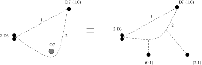
Figure 1: The hypermultiplets from two $D3$ branes and one $D7$ brane.

one obtains two hypermultiplets as desired. For notational purposes we will call this state 1. But there are other possibilities for the compact case where, due to global seven brane charge conservation, we require definite numbers of orientifold planes and seven branes. Now we can have a string that goes all the way across an orientifold plane and comes back to the $D7$ brane (we call this state 2 in the figure). Under non-perturbative corrections, the $O7$ planes will in general split into pairs of seven branes which we denote as (0,1) and (2,1) seven branes, the numbers being the charges measured with respect to axion and dilaton, respectively (in this notation, a $D7$ brane will be denoted as (1,0)). The splitting of the orientifold plane into seven branes create branch cuts on the $\mathbb{P}^{1}$. Therefore the strings reaching the $D7$ brane undergo changes in their charge distribution [50]. If we call the strings leaving from $D3$ as $\pmatrix{1\cr 0}$, then the condition for them to reach the $D7$ brane will be

$$M_{[2,1]}\cdot M_{[0,1]}\cdot\pmatrix{1\cr 0}=\pmatrix{-1\cr~{}0},$$ (3.13)

where $M_{[p,q]}$ are the monodromy matrices whose explicit form can be taken from [50]. One can check that this condition is met for our case. The masses of the strings stretched between the $D3$ branes and $D7$ brane can be calculated and will in general be much heavier than state 1. Some of these states may even be non-BPS. Since all these states are much heavier than the state 1 we can effectively ignore those states for our purposes and concentrate only on the state 1.

Before we end this section, let us mention a few words on the cosmology of this model. One first notes that the $SU(2)$ coupling of the two $D3$ branes (at far distance from $D7$) can no longer be much smaller than the $U(1)$ gauge coupling of the $D7$ brane unless the compactification volume is very small. Hence, the $SU(2)$ gauge symmetry can no longer be treated as effectively global as we mentioned earlier. D-term inflation for such a more complicated gauge group has not yet been studied. Therefore, in this paper, we will focus on a $D3/D7$ brane model with two $D7$ branes and two hypermultiplets in the effective $U(1)$ gauge theory with global $SU(2)$ symmetry.

3.3 Analysis of the warp factor

Now that we have seen how global symmetries and hypermultiplets appear in our setup, it is time to go back to the issue of warp factors that we briefly mentioned at the beginning of this section. Since we have isolated two $D7$ branes from a system of branes and orientifold planes, we have to carefully consider the equation of the warp factor. In the notations that we used above, we keep a probe $D3$ at a point $z={\tilde{z}}_{1}$ on the $\mathbb{P}^{1}$. The two $D7$ branes are located at $z=z_{1}$. The metric ansatz that we used in (3.5) involves two things: (a) the metric on the sphere $\mathbb{P}^{1}$, and (b) the warp factor $\Delta$ (we will not be too concerned with the metric of $K3$ here). Let us first tackle the metric on the $\mathbb{P}^{1}$. In terms of the eta-function $\eta$ we can express the metric near two $D7$ branes on top of each other as [54]:

$$ds^{2}_{\mathbb{P}^{1}}=g_{z\bar{z}}~{}|dz|^{2}\simeq{\rm Im}~{}\tau(z)~{}\big{|}\eta^{2}(\tau)~{}(z-z_{1})^{-{1\over 6}}dz\big{|}^{2}$$ (3.14)

Putting a probe $D3$ brane and additional fluxes only introduces a warp factor $\Delta$ to the system as discussed above in (3.5). The equation for the warp factor can be approximated near the $D7$ branes as:

$$\begin{array}[]{c}\displaystyle{\ast\square~{}\Delta^{2}=~{}~{}H_{NS}\wedge H_{RR}+(4\pi^{2}\alpha^{\prime})^{2}~{}\delta^{2}(z-{\tilde{z}}_{1})~{}\delta^{4}_{K3}+}\\ \\ \displaystyle{~{}~{}~{}~{}~{}+{(\alpha^{\prime}\pi)^{2}\over 64}[{\rm tr}~{}({\cal R}\wedge{\cal R})-{\rm tr}~{}({\cal F}\wedge{\cal F})]~{}\delta^{2}(z-z_{1})}\end{array}$$ (3.18)

where the factor of ${1\over 64}$ comes from the gravitational couplings on the two $D7$ branes. In writing the above relation we have ignored the effect of other seven branes that are placed far away from the two $D7$ branes. The position of the $D3$ brane on the $K3$ is denoted symbolically by the delta function $\delta^{4}_{K3}$.

The solution to the above equation involve various things: (a) the choice of the three forms $H_{NS}$ and $H_{RR}$, (b) the choice of the world volume gauge fluxes ${\cal F}$, and (c) the curvature tensor ${\cal R}$. The full solution to this equation has not been worked out, and therefore we will not try to address it here in details as this would lie beyond the scope of this paper. We only note that an approximate solution to the warp factor can be given in terms of Green’s function à la [55]. Using this one can show that the warp factor is typically of order 1 here as the additional factors are suppressed by the volume of the compact manifold. Since we take large internal volume (which earlier helped us to decouple the seven brane gauge interactions) we can safely ignore the warping effects here. Therefore instead of going to a more detailed analysis of the warp factor, we now turn to the analysis of semilocal strings in this model.

4 Semilocal BPS-strings in supergravity

Semilocal strings are a special class of vortex solutions that were first found in the extended Abelian Higgs model [31, 32]. In that model, the Higgs sector of the conventional Abelian Higgs model (which gives rise to the standard ANO-strings) is doubled so that the theory has a global $SU(2)_{g}$ symmetry, in addition to its local $U(1)_{l}$ gauge symmetry. In the last few sections we saw in detail how the $D3/D7$ system realizes easily the required global and local symmetries of this model, which is the main requirement for the presence of the semilocal strings. However, our model has much more structure, as it is also embedded into $\mathcal{N}=1$ supergravity. In this section, we make use of this extra structure and show how the semilocal strings can arise as $1/2$-BPS solitons in the extended Abelian Higgs model coupled to four-dimensional, $\mathcal{N}=1$ supergravity. While it is known that semilocal strings can satisfy BPS-type energy bounds in the case of critical coupling [31, 32, 34], the precise connection with local supersymmetry has so far not been established in a clear an precise way. Our treatment extends the discussion of ref. [23] for the locally supersymmetric ANO-vortex to the semilocal cosmic string. In the analysis below, we will ignore the effectively decoupled D7 brane gauge fields completely, dropping their kinetic term.

4.1 The Lagrangian

In section 2, we derived the essential features of the low energy effective action of a simple $D3/D7$ brane system in a $K3\times T^{2}/\mathbb{Z}_{2}$ compactification of type IIB string theory (see eq. (2.15) for the $\mathcal{N}=2$ supersymmetric non-gravitational part). As sketched in section 3, this system can be generalized to describe one $D3$ brane near two coincident $D7$ branes with gauge group $U(1)_{l}$ and an effectively global symmetry $SU(2)_{g}$. This global symmetry acts by rotating two (rigid) $\mathcal{N}=2$ hypermultiplets, $\left(\Phi_{+},\Phi_{-}\right)$ and $(\tilde{\Phi}_{+},\tilde{\Phi}_{-})$, into each other. The two hypermultiplets are accompanied by an $\mathcal{N}=2$ vector multiplet $(W_{\mu},S)$ corresponding to the gauged $U(1)_{l}$ symmetry (we are suppressing the fermions for the moment). It can be shown that the neutral and negatively charged scalar fields have to vanish on the string solution [57, 58]. So we will from now on set in this section

$$S=\Phi_{-}=\tilde{\Phi}_{-}=0$$ (4.1)

in equation (3.12). This collapses the superpotential, which we will henceforth set to zero. For the two remaining, positively charged, scalars $\Phi_{+}$ and $\tilde{\Phi}_{+}$, we employ the somewhat more convenient notation

$$\varphi_{1}=\Phi_{+},\qquad\varphi_{2}=\tilde{\Phi}_{+}\ .$$ (4.2)

Coupling this model to gravity reduces supersymmetry to $\mathcal{N}=1$, and the total field content including the fermions now derives from the $\mathcal{N}=1$ supergravity multiplet $(e_{\mu}^{a},\psi_{\mu})$, two chiral multiplets $(\chi_{i},\varphi_{i})$ $(i=1,2)$ and a vector multiplet $(W_{\mu},\lambda)$. Clearly, the two chiral multiplets carry an electric charge $+1$ under the local $U(1)_{l}$ symmetry gauged by $W_{\mu}$ and transform as a doublet under the global $SU(2)_{g}$ symmetry. In the following, we employ the supersymmetry conventions of ref. [16, 56]. In particular, we use $\varphi^{i}$ to denote the complex conjugate of $\varphi_{i}$ and indicate the chirality of their superpartners by $\chi_{i}$ (left handed) and $\chi^{i}$ (right handed).

Taking the Kähler potential and the gauge kinetic function to be minimal, the bosonic part of the Lagrangian then reads

$$e^{-1}{\cal L}_{\rm bos}=-{\textstyle\frac{1}{2}}M_{P}^{2}R-D_{\mu}\varphi_{i}\,D^{\mu}\varphi^{i}-{\textstyle\frac{1}{4}}F_{\mu\nu}F^{\mu\nu}-V^{D}\,,$$ (4.3)

where the D-term potential is defined by

$$V^{D}=\frac{1}{2}D^{2}\qquad D\,=g(\xi-\varphi^{i}\,\varphi_{i})\,$$ (4.4)

and

$$F_{\mu\nu}\equiv{\partial}_{\mu}W_{\nu}-{\partial}_{\nu}W_{\mu}\,,\qquad D_{\mu}\varphi_{i}\equiv({\partial}_{\mu}-{\rm i}gW_{\mu})\varphi_{i}\,$$ (4.5)

denote the usual Abelian field strength and the $U(1)_{l}$ covariant derivative. The transformation rules of the fermions in a purely bosonic background are

$$\delta\psi_{\mu L} = \left(\partial_{\mu}+{\textstyle\frac{1}{4}}\omega_{\mu}{}^{ab}(e)\gamma_{ab}+{\textstyle\frac{1}{2}}{\rm i}A_{\mu}^{B}\right)\epsilon_{L}\,,$$

$$\delta\chi_{i} = {\textstyle\frac{1}{2}}(\not\!{\partial}-{\rm i}g\not\!W)\varphi_{i}\epsilon_{R}\,,$$

$$\delta\lambda = {\textstyle\frac{1}{4}}\gamma^{\mu\nu}F_{\mu\nu}\epsilon+{\textstyle\frac{1}{2}}{\rm i}\gamma_{5}D\epsilon\,.$$ (4.6)

Here the (composite) gravitino $U(1)$ connection, $A_{\mu}^{B}$, is given by

$$A_{\mu}^{B} = \frac{1}{2M_{P}^{2}}{\rm i}\left[\varphi_{i}\partial_{\mu}\varphi^{i}-\varphi^{i}\partial_{\mu}\varphi_{i}\right]+\frac{1}{M_{P}^{2}}W_{\mu}D$$ (4.7)

$$= \frac{1}{2M_{P}^{2}}{\rm i}\left[\varphi_{i}D_{\mu}\varphi^{i}-\varphi^{i}D_{\mu}\varphi_{i}\right]+\frac{g}{M_{P}^{2}}W_{\mu}\xi\,.$$

4.2 Semilocal vortices with unbroken supersymmetry

Our goal here is to show how the above action can give rise to string-like defect solution that preserve one half of the original $\mathop{\mathcal{N}}=1$ supersymmetry. For simplicity, we restrict ourselves to non-singular configurations that are static and cylindrically symmetric, that is, we assume $(1+1)$-dimensional Poincaré symmetry on the ‘world sheet’ of the string as well as a rotational symmetry with orbits orthogonal to that world sheet. Using $(t,z)$ as the world sheet coordinates, we align the rotation axis of the string with the $z$-direction. The orthogonal distance from the rotation axis is denoted by $r$ and rotations about the axis are parameterized by an angular coordinate $\theta$. The space-time metric can be brought to the form

$${\rm d}s^{2}=-{\rm d}t^{2}+{\rm d}z^{2}+{\rm d}r^{2}+C^{2}(r){\rm d}\theta^{2}\,.$$ (4.8)

We use the vierbein with $e^{1}={\rm d}r$ and $e^{2}=C(r){\rm d}\theta$, which leads to the spin connection

$$\omega_{r}{}^{12}=0\,,\qquad\omega_{\theta}{}^{12}=-C^{\prime}(r)\,.$$ (4.9)

In order for the string to have finite energy per unit length, the potential and kinetic energy densities have to vanish sufficiently fast at large distances $r$ from the string axis. As for the potential energy, this means that the scalar fields $\varphi_{i}$ have to approach the vacuum manifold $S^{3}=\{\varphi_{i}:|\varphi_{1}|^{2}+|\varphi_{2}|^{2}=\xi\}$ of the potential $V^{D}$ as $r\rightarrow\infty$. A cosmic string in this model thus defines a mapping of the spatial circle $S^{1}_{\infty}$ at infinite $r$ into the vacuum manifold $S^{3}$.

If this was the only condition, one would conclude that there could be no topologically non-trivial vortices, as $\pi_{1}(S^{3})$={1}, i.e., any non-trivial mapping of $S^{1}_{\infty}$ could be deformed into the trivial map (i.e., the vacuum) at no cost of potential energy.

As was pointed out in [31, 32], however, the requirement of finite kinetic energy per unit length is of equal importance, as it implies that $D_{\mu}\varphi_{i}$ also vanish sufficiently fast at large $r$. This further restricts $(\varphi_{1},\varphi_{2})$ to approach a $U(1)_{l}$ gauge orbit (i.e., a great circle $S^{1}_{l}$) on $S^{3}$ as $r$ goes to infinity. The Higgs field $(\varphi_{1},\varphi_{2})$ at $r\rightarrow\infty$ thus really defines a map of $S^{1}_{\infty}$ into a gauge orbit $S^{1}_{l}$ of $U(1)_{l}$ on the vacuum manifold $S^{3}$. Any such map is characterized by a winding number $n\in\pi_{1}(S^{1}_{l})=\mathbb{Z}$ and an associated gauge connection that compensates the gradient energy from the angular dependence of the Higgs field. Stokes’s theorem and the requirement that $D_{\mu}\varphi_{i}\rightarrow 0$ as $r\rightarrow\infty$ then imply the presence of a magnetic flux through the $(r,\theta)$ plane:

$$\oint_{S^{1}_{\infty}}W_{\theta}d\theta=2\pi n\,.$$ (4.10)

As there are no gauge orbits perpendicular to the $U(1)_{l}$ gauge orbits (because $SU(2)_{g}$ is not gauged), any collective motion off such a $U(1)_{l}$ orbit (i.e., any unwinding of the string at infinity) would cost an infinite amount of gradient energy which could not be compensated for by an appropriate gauge connection. Thus, it is really the fundamental group of a gauge orbit $S^{1}_{l}$ on the vacuum manifold that matters for the stability against unwinding and not the naive fundamental group of the vacuum manifold $S^{3}$ itself [31, 32].

It is important to note, however, that the stability against unwinding (i.e., the conservation of the total magnetic flux as a topological invariant) does not necessarily mean that such defects are stable against other types of deformations. In particular, the magnetic flux need not be confined or localized in a small or thin region of spacetime, but may spread out to fill larger regions (while still being globally conserved). As was pointed out in [32, 33, 35], topological defects may be unstable against such ‘spreading’ if the full vacuum manifold is a non-trivial fiber bundle over a base manifold with the gauge orbit as the fiber such that the relevant homotopy group of the total bundle becomes trivial. To translate this to our situation, one notes that $S^{3}$ is a nontrivial $S^{1}_{l}$ bundle over $\mathbb{C}\mathbb{P}^{1}\cong S^{2}$, and $\pi_{1}(S^{3})=\{1\}$, whereas $\pi_{1}(S^{1}_{l})=\mathbb{Z}$. As we will see shortly, in our model this phenomenon manifests itself in the form of zero modes that describe a possible fattening and warping of the magnetic flux tube. This ability to spread out the flux is one of the properties that make these semilocal strings more appealing in a cosmological context, see the discussion in section 5.

Let us now describe the semilocal string solutions of our model in more detail. The above-mentioned asymptotic behavior for $r\rightarrow\infty$ and the cylindrical symmetry imply that $\Phi(r,\theta)\equiv(\varphi_{1}(r,\theta),\varphi_{2}(r,\theta))$ approaches a field configuration of the form

$$\Phi(r,\theta)\longrightarrow\Phi_{0}e^{in\theta},\qquad r\longrightarrow\infty$$ (4.11)

where $\Phi^{\dagger}_{0}\Phi_{0}=\xi$. The global $SU(2)_{g}$ symmetry allows us to align $\Phi_{0}$ with the $\varphi_{1}$ direction, and the most general Higgs field configuration consistent with cylindrical symmetry is then

$$\left(\begin{array}[]{c}\varphi_{1}(r,\theta)\\ \varphi_{2}(r,\theta)\end{array}\right)=\left(\begin{array}[]{c}f(r)e^{in\theta}\\ h(r)e^{im\theta}\end{array}\right),$$ (4.12)

whereas the gauge potential takes the form

$$gW_{\mu}\,{\rm d}x^{\mu}=n\alpha(r)\,{\rm d}\theta\,\quad\rightarrow\quad F={\textstyle\frac{1}{2}}F_{\mu\nu}\,{\rm d}x^{\mu}\,{\rm d}x^{\nu}={n\alpha^{\prime}(r)\over g}{\rm d}r\,{\rm d}\theta={n\alpha^{\prime}(r)\over gC(r)}e^{1}e^{2}\,.$$ (4.13)

Here, $f(r)$, $h(r)$ and $\alpha(r)$ are the profile functions of the Higgs fields and the vector field, whereas $m$ is an a priori arbitrary integer.

The desired asymptotic behavior at $r\rightarrow\infty$ and the assumed non-singular behavior at the origin impose the following boundary conditions on the functions $f(r)$, $h(r)$, $\alpha(r)$ and the metric function $C(r)$:

$$C(0)=0, C^{\prime}(0)=1$$

$$f(0)=0, f(r)\longrightarrow\sqrt{\xi}\quad\textrm{ as }r\longrightarrow\infty$$

$$h(0)=h_{0}\delta_{m0}, h(r)\longrightarrow 0\quad\,\,\,\,\,\,\textrm{ as }r\longrightarrow\infty$$

$$\alpha(0)=0, \alpha(r)\longrightarrow 1\quad\,\,\,\,\,\,\textrm{ as }r\longrightarrow\infty$$ (4.14)

where we have indicated that $h(0)$ might be non-zero for $m=0$, with $h_{0}$ being some constant.

Our goal now is to find profile functions $f(r)$, $h(r)$, $\alpha(r)$, $C(r)$, which describe a solution of the Lagrangian that preserves $1/2$ of the original supersymmetry. We thus have to find an appropriate Killing spinor $\epsilon(r,\theta)$ such that $\delta\psi_{\mu}=\delta\chi_{i}=\delta\lambda=0$ can be satisfied for a certain form of the profile functions. For simplicity, we will from now on assume

$$n>0\,.$$ (4.15)

In order to cancel the magnetic flux contribution to $\delta\lambda$, we choose the following projector for the Killing spinor

$$\gamma^{12}\epsilon\,=\,-{\rm i}\gamma_{5}\epsilon\,.$$ (4.16)

The BPS equations that follow from the vanishing of the transformation rules (4.6) for the chiral fields $\chi_{i}$ and for the gaugino $\lambda$ are then

$$\Bigl{(}C(r){\partial}_{r}\,+\,{\rm i}\,({\partial}_{\theta}-{\rm i}gW_{\theta})\Bigr{)}\varphi_{i}\,=\,0\,,$$

$$F_{12}\,-D\,=\,0\,,$$ (4.17)

which leads to

$$C(r)f^{\prime}(r) = n\left[1-\alpha(r)\right]f(r),$$ (4.18)

$$C(r)h^{\prime}(r) = \left[m-n\alpha(r)\right]h(r),$$ (4.19)

$$\alpha^{\prime}(r) = \frac{g^{2}C(r)}{n}\left[\xi-f^{2}(r)-h^{2}(r)\right].$$ (4.20)

These three equations are not completely independent, as solving eqs. (4.18) and (4.19) for $\alpha(r)$ and equating both expressions yields the relation

$$\partial_{r}\ln\left(\frac{h(r)}{f(r)}\right)=\frac{m-n}{C(r)}.$$ (4.21)

We make further use of this relation in Section 2.3 to derive an upper bound on the possible integers $m$.

It remains to determine the gravitino BPS equation, for which one needs the composite connection $A_{\mu}^{B}$:

$$A_{r}^{B}=0\,,\qquad A_{\theta}^{B}=\frac{1}{M_{P}^{2}}\left[nf^{2}(r)+mh^{2}(r)+n\alpha(r)\left(\xi-f^{2}(r)-h^{2}(r)\right)\right].$$ (4.22)

The gravitino BPS equation is now

$$\partial_{r}\epsilon=0\,,\qquad\left[\partial_{\theta}+{\textstyle\frac{1}{2}}iC^{\prime}(r)+{\textstyle\frac{1}{2}}{\rm i}A_{\theta}^{B}\right]\epsilon_{L}(\theta)=0\,.$$ (4.23)

The $\theta$ dependence of $\epsilon$ follows from the limit $r\rightarrow 0$, where $A_{\theta}^{B}$ goes to zero and $C^{\prime}(r)$ approaches $1$ so that (4.23) implies

$$\epsilon_{L}(\theta)={\rm e}^{-{\textstyle\frac{1}{2}}{\rm i}\theta}\epsilon_{0L}\,,$$ (4.24)

where $\epsilon_{0L}$ is the left handed part of a constant spinor satisfying the projection equation (4.16). Thus, the gravitino equation $\delta\psi_{\mu}=0$ boils down to

$$1-C^{\prime}(r)=A_{\theta}^{B}\,.$$ (4.25)

with $A^{B}_{\theta}$ as in (4.22).

4.3 Limiting cases

While no analytic solution to the BPS equations (4.18) – (4.20), (4.25) is known, a great deal of physical information can already be obtained by studying the limiting behavior at $r=0$ and $r\rightarrow\infty$.

We will first show how the limiting behavior constrains the possible integers $m$ in $\varphi_{2}(r,\theta)$. In the limit where $r$ approaches zero, $C(r)=r+\mathcal{O}(r^{2})$ (see eqs. (4.14)). As $\alpha(r)$ must be at least of linear order in $r$, the $\alpha$-term in the BPS equations (4.18) and (4.19) can be neglected to lowest order in $r$. To lowest non-trivial order, these two equations thus read

$$rf^{\prime}(r) = nf(r)$$ (4.26)

$$rh^{\prime}(r) = mh(r)$$ (4.27)

whence

$$f(r)=f_{n}r^{n}+\mathcal{O}(r^{n+1}),\qquad h(r)=h_{m}r^{m}+\mathcal{O}(r^{m+1})$$ (4.28)

with some non-vanishing coefficients $f_{n}$, $h_{m}$ ($h_{m}$ might be zero for $m=0$). Finiteness of $h(r)$ at $r=0$ then implies $m\geq 0$.

To derive also an upper limit on $m$, consider eq. (4.21). As $h(r)/f(r)\rightarrow 0$ for $r\rightarrow\infty$, the left hand side of (4.21) has to be negative, which, because of the positivity of $C(r)$ implies that $m<n$. We have thus obtained the bounds

$$0\leq m<n.$$ (4.29)

Let us now take a closer look at the limiting behavior at large $r$. As $r$ approaches infinity, $(f(r),h(r),\alpha(r))$ approach their asymptotic values $(\sqrt{\xi},0,1)$. It is easy to see, that the four BPS-equations are consistent with this behavior provided that asymptotically

$$C(r)\sim r\left(1-\frac{n\xi}{M_{P}^{2}}\right)\,.$$ (4.30)

This shows that asymptotically the string creates a locally-flat conical metric with an angular deficit angle which is due to the constant FI term $\xi$:

$${\rm d}s^{2}=-{\rm d}t^{2}+{\rm d}z^{2}+{\rm d}r^{2}+r^{2}\left(1-\frac{n\xi}{M_{P}^{2}}\right)^{2}{\rm d}\theta^{2}\,.$$ (4.31)

Notice also that in the limit $r\rightarrow\infty$ the full supersymmetry is restored because $F_{\mu\nu}=0$, $D=0$, $\partial_{r}\varphi_{i}=D_{\theta}\varphi_{i}=0$ and $R_{\mu\nu}{}^{ab}=0$ which corresponds to the enhancement of supersymmetry away from the core of the string. This is the same result as for the standard ANO vortex [23], however, it should be pointed out that the rate at which the asymptotic values of the profile functions $f(r)$, $h(r)$ and $\alpha(r)$ are obtained is in general no longer described by an exponential fall-off, but can change into a power law behavior depending on the values of certain moduli parameters of the semilocal string [32] . To understand this better, let us now turn to the behavior at small $r$.

Expanding the profile functions as power series of the form $f(r)=f_{0}+f_{1}r+f_{2}r^{2}+\ldots$ and similarly for $h(r)$, $\alpha(r)$ and $C(r)$, we know already that

$$f(r) = f_{n}r^{n}+\mathcal{O}(r^{n+1})$$ (4.32)

$$h(r) = h_{m}r^{m}+\mathcal{O}(r^{m+1})$$ (4.33)

$$C(r) = r+\mathcal{O}(r^{2})$$ (4.34)

In order to determine the lowest non-trivial power of $\alpha(r)$, we expand (4.20) to lowest order and obtain

$$\alpha(r)=\alpha_{2}r^{2}+\mathcal{O}(r^{3}),\qquad\textrm{ with }\qquad\alpha_{2}=\frac{g^{2}}{2n}[\xi-h_{0}^{2}]\,.$$ (4.35)

In a similar fashion one can now determine the higher coefficients order by order and arrives at recursion relations that determine all coefficients in terms of $\xi$ and the lowest non-trivial coefficients $f_{n}$ and $h_{m}$ of the Higgs fields. It is easy to see that the recursion relations are such that $f(r)$ contains only odd powers when $n$ is odd and only even powers when $n$ is even. Similarly, the function $h(r)$ is odd/even if $m$ is odd/even. $\alpha(r)$, by contrast is always even, whereas $C(r)$ only contains odd powers.

This power series expansion leaves the lowest Higgs coefficients $f_{n}$ and $h_{m}$ undetermined. In fact, the coefficient $h_{m}$ turns out to be a undetermined parameter of the solution, whereas $f_{n}$ can be fixed numerically by matching to the required asymptotic behavior at infinity. The numerical value of $f_{n}$ depends upon the parameter $h_{m}$.

The parameters $h_{m}$ can actually be taken to be complex, as one has the freedom to shift the phase of $\varphi_{2}=h(r)e^{im\theta}$ by a constant shift and absorb that phase into $h_{m}$. If one breaks the rotational invariance by either allowing linear combinations $\varphi_{2}(r,\theta)=\sum_{m=0}^{n-1}h^{(m)}(r)e^{im\theta}$ and/or by splitting an $n$-vortex into (up to $n$) vortices with smaller winding numbers and different positions in the $(r,\theta)$ plane, one expects supersymmetry to be preserved and finally arrives at a $2n$-complex-dimensional moduli space of semilocal vortices [34].

The physical interpretation of the moduli $h_{m}$ can most easily be illustrated for the parameter $h_{0}$ in the case $m=0$. In that case, eqs. (4.35) and (4.13) yield the magnetic field

$$F_{12}(0)=g(\xi-h_{0}^{2})$$ (4.36)

at the origin. In the limit $h_{0}\rightarrow 0$ this approaches the magnetic field in the core of the ANO-string [23]. This is not surprising, as $h_{0}=0$ implies $h(r)\equiv 0$ in the case of $m=0$ via the recursion relations that follow from the BPS equations. In that case, the BPS equations reduce to those of the ANO-string.

On the other hand, increasing $h_{0}$ from $0$ to $\sqrt{\xi}$, decreases the magnetic field in the core. As the total flux only depends on the winding number $n$, and thus is unaffected by changes in $h_{0}$, this means that the flux tube must become flatter and wider. Thus, $h_{0}$ is a measure for the width of the magnetic flux tube and encodes the possibility for semilocal strings to spread out their flux into larger space-time regions [32].

Another interesting quantity is the spacetime curvature $R=2C^{\prime\prime}/C$ in the center of the string. At $r=0$, this quantity reduces to $R(0)=12C_{3}$. $C_{3}$ can be easily obtained from the first non-trivial power of eq. (4.25), which leads to

$$R(0)=-4\left(\frac{f_{1}}{M_{P}}\right)^{2}-2\left(\frac{g(\xi-h_{0}^{2})}{M_{P}}\right)^{2}$$ (4.37)

We finally note that for high $n$ and $m$, the functions $f(r)$ and $h(r)$ are zero at least up to order $r^{m}$ (remembering $m<n$). Up to terms of order $r^{2m}$, the BPS equations (4.20) and (4.25) then simplify to

$$\alpha^{\prime}(r)=\frac{g^{2}\xi}{n}C(r)\,,\qquad 1-C^{\prime}(r)-nM_{P}^{-2}\xi\alpha(r)=0\,,$$ (4.38)

which, in view of the boundary conditions at $r=0$, can be solved as

$$\alpha(r) = \frac{M_{P}^{2}}{n\xi}\Bigl{(}1-\cos({g\xi\over M_{P}}r)\Bigr{)},$$

$$C(r) = {M_{P}\over\xi g}\sin({g\xi\over M_{P}}r)\,.$$ (4.39)

Up to terms of order $r^{2m+1}$, the metric at small $r$ is then:

$${\rm d}s^{2}=-{\rm d}t^{2}+{\rm d}z^{2}+{\rm d}r^{2}+\left[{M_{P}\over\xi g}\sin({g\xi\over M_{P}}r)\right]^{2}{\rm d}\theta^{2}\,,$$ (4.40)

whereas, up to terms of order $r^{m}$ for the Higgs and $r^{2m+2}$ for the gauge fields, one obtains

$$\varphi_{i}=0\,,\qquad W_{\theta}=\frac{M_{P}^{2}}{g\xi}\Bigl{(}1-\cos({g\xi\over M_{P}}r)\Bigr{)}\,,\qquad F_{r\theta}=M_{P}\sin({g\xi\over M_{P}}r)\,.$$ (4.41)

5 Cosmology and semilocal strings

5.1 Inflation

The semilocal strings embedded into supergravity were shown in the previous section to have an unbroken supersymmetry for a continuous range of the parameter $h_{0}$, which effectively measures the width of the flux tube and is not defined by the parameters in the action. Now we would like to study the properties of the semilocal strings in applications to cosmology.

The generalized D-term model after doubling the number of hypermultiplets corresponding to doubling the number of $D7$ branes in the $D3/D7$ model has the following potential:

$$V = \frac{g^{2}}{2}\left|\phi_{+}\phi_{-}-\tilde{\phi}_{-}\tilde{\phi}_{+}\right|^{2}+\frac{g^{2}}{8}\left[|\phi_{+}|^{2}+|\tilde{\phi}_{+}|^{2}-|\phi_{-}|^{2}-|\tilde{\phi}_{-}|^{2}-2\xi\right]^{2}+$$ (5.1)

$$\frac{g^{2}}{2}|s|^{2}\left[|\phi_{+}|^{2}+|\phi_{-}|^{2}+|\tilde{\phi}_{+}|^{2}+|\tilde{\phi}_{-}|^{2}\right].$$

Here all scalar fields have canonical kinetic terms, such as ${1\over 2}(\partial\phi)^{2}$. They are related to the chiral fields in the action (5.1) as follows: $\phi_{+}=\sqrt{2}\,\Phi_{+},s=\sqrt{2}\,S$ etc. The tree-level potential (5.1) has a supersymmetric minimum (a valley with $V=0$):

$$s=0\ ,\qquad\left|\phi_{+}\phi_{-}-\tilde{\phi}_{+}\tilde{\phi}_{-}\right|\ =\ 0\ ,$$

$$|\phi_{+}|^{2}+|\tilde{\phi}_{+}|^{2}-|\phi_{-}|^{2}-|\tilde{\phi}_{-}|^{2}\ =\ 2\xi\ .$$ (5.2)

The $U(1)$ gauge symmetry is broken in the minimum. In the absence of strings, the fields can take any values along this valley. When strings are present, the fields tend to drift towards the state with $\phi_{-}=\tilde{\phi}_{-}=0$, because $\phi_{-}=\tilde{\phi}_{-}=0$ for the BPS (lowest energy state) solutions [57, 58].

The potential has a second flat direction, $\phi_{\pm}=\tilde{\phi}_{\pm}=0$. Inflation occurs when the field $s$ rolls along this flat direction. At the classical level, the scalar potential (5.1) equals $\frac{g^{2}}{2}\xi^{2}$ for all values of $s$ at $\phi_{\pm}=\tilde{\phi}_{\pm}=0$; in order to study inflationary dynamics one should take into account one-loop corrections to the effective potential.

We will consider the models with $g^{2}\mathrel{\hbox{\hbox to0.0pt{\hbox{\lower 4.0pt\hbox{$\sim$}}\hss}\hbox{$>$}}}10^{-4}$, because it is more difficult to motivate much smaller coupling constant $g^{2}$ in string theory. As we will see, inflation in the model with $g^{2}\mathrel{\hbox{\hbox to0.0pt{\hbox{\lower 4.0pt\hbox{$\sim$}}\hss}\hbox{$>$}}}10^{-4}$ ends at $s\gg s_{c}=\sqrt{\xi}$. In this regime, the one-loop corrected potential of the field $s$ in the model with $C$ hypermultiplets of equal $g^{2}$ is given by [17, 30]

$$V_{\rm eff}=\frac{g^{2}}{2}\xi^{2}\left\{1+\frac{Cg^{2}}{8\pi^{2}}\left[\ln\frac{s^{2}}{s_{c}^{2}}\right]\right\}\ .$$ (5.3)

To study inflation, one should use the Friedmann equation

$$H={\dot{a}\over a}\approx\sqrt{V/3}\approx{g\xi\over\sqrt{6}}\ ,$$ (5.4)

where $a(t)$ is a scale factor of the universe. This leads to inflation

$$a(t)=a(0)~{}\exp{{{g\xi\ t\over\sqrt{6}}}}~{}.$$ (5.5)

During the slow-roll regime, the field $s$ obeys equation $3H\dot{s}=-V^{\prime}(s)$ [60], which gives

$$s^{2}(t)=s^{2}(0)-{Cg^{3}\xi~{}t\over 2\sqrt{6}\pi^{2}}\ .$$ (5.6)

Using equations (5.5), (5.6) one can find the value of the field $s_{{}_{N}}$ such that the universe inflates $e^{N}$ times when the field rolls from $s_{{}_{N}}$ to the bifurcation point $s=s_{c}$:

$$s_{{}_{N}}^{2}={s_{c}}^{2}+{Cg^{2}N\over 2\pi^{2}}={\xi}+{Cg^{2}N\over 2\pi^{2}}\ .$$ (5.7)

In this paper we will concentrate on the case ${Cg^{2}\over 2\pi^{2}}>\xi$. Density perturbations on the scale of the present cosmological horizon have been produced at $s\sim s_{N}\gg s_{c}$ with $N\sim 60$, and their amplitude is proportional to ${V^{3/2}\over V^{\prime}}$ at that time [60]. One can find $\xi$ using the COBE normalization for inflationary perturbations of the metric on the horizon scale [27]:

$$\delta_{H}={1\over 5\sqrt{3}\pi}{V^{3/2}\over V^{\prime}}\approx 1.9\times 10^{-5}\ .$$ (5.8)

This yields

$${V^{3/2}\over V^{\prime}}={2\sqrt{2}\pi^{2}\xi\over Cg}~{}s_{{}_{N}}\sim 2\pi\xi\sqrt{N\over C}\sim 5.2\times 10^{-4}\ .$$ (5.9)

In what follows, we will concentrate on the case with two hypermultiplets and take $N=60$. In this case

$$\xi\sim{5.2\times 10^{-4}\over 2\pi}\sqrt{C/N}\sim 1.5\times 10^{-5}\ .$$ (5.10)

This yields the scale of spontaneous symmetry breaking

$$\sqrt{\xi}\sim 9.3\times 10^{15}\,{\rm GeV}.$$ (5.11)

This model has a nearly flat spectrum of density perturbations, $n\approx 0.98$, and a very small amplitude of gravitational waves. Both of these features are in a good agreement with the observational data.

5.2 Semilocal strings in cosmology

After the field $s$ passes the bifurcation point $s_{c}=\sqrt{\xi}$, the fields $\phi_{\pm},\tilde{\phi}_{\pm}=0$ start rolling to the minimum of the effective potential at $|\phi_{+}|^{2}+|\tilde{\phi}_{+}|^{2}-|\phi_{-}|^{2}-|\tilde{\phi}_{-}|^{2}\ =\ 2\xi$. This leads to production of cosmic strings. One should check whether the semilocal cosmic strings produced during this process can affect the amplitude of large-scale density perturbations.

Cosmic strings lead to perturbations of the metric with flat spectrum if in the course of the evolution of the universe there always remains at least one string of length comparable to the size of the particle horizon $\sim ct$ [61]. We will call such strings infinite. Thus one needs to check whether infinite semilocal strings can form and survive long after the end of inflation.

This issue is rather nontrivial. Even though stability of semilocal strings is not protected by topological considerations, one could argue that infinitely long straight strings are protected because they are BPS solutions, so their energy cannot get any lower. On the other hand, the fact that the thin and thick BPS strings have the same tension indicates that strings can be unstable if it is possible to excite a zero mode which would lead to the growth of their thickness; see e.g. [32, 33, 34]. However, it would require infinite action to excite such a zero mode in an infinitely large universe [34]. Also, the growth of thickness of a single infinite string occurs with the speed smaller than the speed of light, and the string tension does not change in this process. Meanwhile (however strange this might seem), the diameter of the observable part of the universe grows with the speed 4 times greater than the speed of light in a universe dominated by ultrarelativistic particles, and with the speed 6 times greater than the speed of light in the cold dark matter dominated universe [60]. Thus, on the horizon scale, each separate infinite semilocal string will always look thin, and its expansion will not lead to the change of its tension. This means that the spreading of each individual BPS string would not change the amplitude of density perturbations which it produces.

However, the strings created at the end of inflation initially are not straight, infinite BPS strings. In contrast to the case of the standard Nielsen-Olesen cosmic strings, infinite semilocal strings do not appear at the moment of the phase transition. Typically, soon after the phase transition, strings look like a cloud of string segments of a size comparable to the correlation length at the moment of the cosmological phase transition. These string segments have global monopoles at their ends. Each global monopole attracts a nearby global anti-monopole with a force that does not depend on the distance between them. If the monopole and the antimonopole closest to it belong to the ends of two different strings, they attract each other, and the two strings tend to merge, forming one longer string. However, if a string is shorter than the distance between it and another string, the two monopoles on its ends are attracted to each other stronger than to other monopoles. As a result, either such short string segment shrinks and disappears due to its tension and monopole interactions, or in the beginning it forms a small loop, and then the loop shrinks and disappears.

Infinite semilocal strings responsible for the large scale density perturbations can appear only because of merging of short string segments. The probability of this process is expected to be small; it is not reinforced by topological considerations. In addition, the possibility of growth of thickness of the near-BPS string segments eventually may lead to their overlapping with other string segments, which may result in their de-localization and effective disappearance. (Note that it does not cost infinite energy or infinite action to excite the zero mode for each segment of a semilocal near-BPS string of a finite size.) A numerical investigation of this process was performed in [37], with the conclusion that infinite semilocal BPS strings are not formed, and therefore they do not lead to the problem of excessively large string-related metric perturbations.

One should exercise some caution before applying the results of Ref. [37] to the model (5.1). Indeed, numerical simulations performed in Ref. [37] did not fully take into account the quantum dynamics of spontaneous symmetry breaking in hybrid inflation. Instead of that, the authors simply made some plausible assumptions about the random distribution of the scalar field after the phase transition. Then they verified that their results are not very sensitive to these assumptions, but in their analysis they did not take into account the expansion of the universe. Also, the numerical analysis was performed in [37] for a simpler model, which did not contain the fields $\phi_{-},\tilde{\phi}_{-}$. One could argue [30] that these fields are not important because eventually the fields drift towards the state with $\phi_{-}=\tilde{\phi}_{-}=0$ since $\phi_{-}=\tilde{\phi}_{-}=0$ for the BPS solutions [57, 58]. The short string segments produced after inflation initially are not in the BPS state, and the process of disappearance of the fields $\phi_{-}=\tilde{\phi}_{-}=0$ could take a very long time [57], but the numerical simulations performed in [59] suggest that this time can be rather short.

We do believe that the results obtained in [37, 59] provide a strong evidence that the semilocal strings formed in the model (5.1) do not pose any cosmological problems, but the importance of this subject warrants its full quantum mechanical analysis. This can be done using the methods of Ref. [39], where the process of spontaneous symmetry breaking in the simplest versions of hybrid inflation was investigated. These methods allow to perform a complete quantum field theory investigation of string formation in the early universe [62]. Leaving this full analysis for a future investigation, we will discuss some important features of the processes which occur after inflation in the model (5.1). We will argue that the expansion of the universe does not lead to qualitative changes in the processes studied in [37], and that in the first approximation one can indeed ignore the effects related to the fields $\phi_{-},\tilde{\phi}_{-}$. Our analysis will provide a framework for the future numerical investigation of this issue.

5.3 Symmetry breaking and string formation at the end of inflation

According to [17, 30], the field $s$ at the last stages of inflation rolls down along the valley with $\phi_{\pm},\tilde{\phi}_{\pm}=0$ until it reaches the bifurcation point $s_{c}=\sqrt{\xi}$. Then it continues rolling along the ridge with $\phi_{\pm},\tilde{\phi}_{\pm}=0$ until the fields fall down from the ridge and spontaneous symmetry breaking occurs. When the fields $\phi_{\pm},\tilde{\phi}_{\pm}$ acquire nonvanishing (complex) expectation values, their initial distribution looks very chaotic, which can lead to string formation via the Kibble mechanism.

Even though the discussion of spontaneous symmetry breaking can be found in every book of quantum field theory, the dynamics of this process was understood only very recently, and the results were rather surprising [39]. For example, one could expect that when the fields fall down from the top of the effective potential to its minimum at $\phi\sim\sqrt{2\xi}$, they should enter a long stage of oscillations with the amplitude $\sim\sqrt{2\xi}$. However, a detailed investigation of this issue shows that because of the exponential growth of quantum fluctuations in the process of spontaneous symmetry breaking, the main part of the kinetic energy of the rolling fields becomes converted into the gradient energy of the inhomogeneous distribution of these fields within a single oscillation. The resulting distribution looks like a collection of classical waves of scalar fields moving near the minimum of the effective potential, the amplitude of these waves being much smaller than the amplitude of spontaneous symmetry breaking $\sqrt{2\xi}$. In other words, the main part of the process of symmetry breaking completes within a single oscillation of the field distribution [39].

In order to study this process in the context of the model (5.1), we need to know the speed of rolling of the field $s$ as it passes the bifurcation point $s_{c}$. This will allow us to find how far along the ridge the field $s$ can go until spontaneous symmetry breaking occurs. The estimates we are going to make will be very rough, but sufficient for our purposes.

According to (5.7) and (5.10), for $C=2$ and $g^{2}\gg 10^{-4}$ the slow-roll regime ends not at the bifurcation point, but earlier, at $s_{1}\sim{g\over\pi}\gg s_{c}$. At $s<s_{1}$ the field rolls down very fast, reaching the bifurcation point $s_{c}$ within the time smaller than the Hubble time $H^{-1}$. Therefore during this time the total energy density of the field $s$ is (approximately) conserved. This leads to an estimate ${1\over 2}\dot{s}^{2}\sim{g^{4}\xi^{2}\over 16\pi^{2}}\ln{g^{2}\over\pi^{2}\xi}$ for the velocity of the field $s$ at the bifurcation point.

Symmetry breaking happens at $s<s_{c}$ because the fields $\phi_{+},\tilde{\phi}_{+}$ acquire the tachyonic mass at $s<s_{c}$,

$$m_{+}^{2}=g^{2}(s^{2}-s_{c}^{2})<0\ .$$ (5.12)

This means that, after passing the bifurcation point, the tachyonic mass of the fields $\phi_{+},\tilde{\phi}_{+}$ grows as follows:

$$m_{+}^{2}\approx-2g^{2}\sqrt{\xi}\Delta s=g^{2}\sqrt{\xi}\,\dot{s}\,\Delta t\ ,$$ (5.13)

where $\Delta s=s_{c}-s$.

The process of spontaneous symmetry breaking occurs because of the exponential growth of quantum fluctuations of the fields with a tachyonic mass. Ignoring, in the first approximation, the time dependence of the tachyonic mass, one can find that quantum fluctuations of the fields with $m_{+}^{2}<0$ and momentum $k<|m_{+}|$ grow exponentially:

$$\delta\phi_{+}\sim\delta\tilde{\phi}_{+}\sim e^{i\sqrt{m_{+}^{2}+k^{2}}\ t}\sim e^{\sqrt{|m_{+}^{2}|-k^{2}}\ t}$$ (5.14)

Occupation numbers of quantum fluctuations grow as $e^{2\sqrt{|m_{+}^{2}|-k^{2}}\ t}$. When the occupation numbers become much greater than 1, growing quantum fluctuations can be interpreted as a classical scalar field. This means that the growing components of the scalar fields $\phi_{+},\tilde{\phi}_{+}$ will look inhomogeneous on the scale $|m_{+}|^{-1}$. The average initial amplitude of quantum fluctuations with $k<|m_{+}|$ is $O(10^{-1}|m_{+}|)$ [39]. Because of the exponential character of the growth, it takes the field distribution the time $\sim|m_{+}|^{-1}\ln{10\sqrt{\xi}\over|m_{+}|}$ before it reaches the minimum of the effective potential. In fact, the total duration will be somewhat smaller because the curvature of the effective potential grows in the process.

Note that in our case $|m_{+}|$ is vanishingly small at the bifurcation point; it becomes large only later. Therefore spontaneous symmetry breaking occurs only when the time that it takes for the rolling field $s$ to reach some point $s<s_{c}$ becomes comparable to $|m_{+}(s)|^{-1}\ln{10\sqrt{\xi}\over|m_{+}(s)|}$. This condition reads

$$2g^{2}\sqrt{\xi}\ \Delta s\ln^{-2}{10\sqrt{\xi}\over|m_{+}(s)|}\sim{\dot{s}^{2}\over(\Delta s)^{2}}\sim{g^{4}\xi^{2}\ln{g^{2}\over\pi^{2}\xi}\over 8\pi^{2}(\Delta s)^{2}}.$$ (5.15)

To find an approximate solution of this equation, we will take $|m_{+}(s)|=|m_{+}(0)|=g\sqrt{\xi}$ under the logarithm. This yields

$$\Delta s\sim F(g)\ g^{2/3}\sqrt{\xi}\ ,$$ (5.16)

where

$$F(g)=\left({\ln{g^{2}\over 4\pi\xi}\ln^{2}{10^{2}\over g^{2}}\over 64\pi^{2}}\right)^{1/3}.$$ (5.17)

Numerical evaluation of this expression shows, for example, that $F\sim 0.8$, and $\Delta s\sim 0.2\,s_{c}$ for $g^{2}\sim 10^{-2}$. Finally, we find the absolute value of the tachyonic mass of the fields $\phi_{+},\tilde{\phi}_{+}$ at the moment when the symmetry breaking occurs:

$$|m_{+}|\sim 2^{1/4}F^{1/2}(g)\ g^{4/3}\sqrt{\xi}\ =O(g^{4/3}\sqrt{\xi})\ .$$ (5.18)

Note that at this stage the only fluctuations experiencing the tachyonic growth are those of the fields $\phi_{+},\tilde{\phi}_{+}$; the fields $\phi_{-},\tilde{\phi}_{-}$ are not generated. On average, the amplitude of the complex fields $\phi_{+}$ and $\tilde{\phi}_{+}$ should be the same, but in different parts of the universe separated by a distance more than $m_{+}^{-1}$ the values of these fields as well as their phases can be different. Therefore the correlation length which determines the typical initial length of the string segments and the typical initial distance between the cosmic strings is expected to be

$$\Delta x=O(g^{4/3}\sqrt{\xi})\ .$$ (5.19)

For the range of parameters we are interested in, this correlation length can be two orders of magnitude smaller than the horizon size at that time, $H^{-1}\sim g^{-1}\,\xi^{-1}$, which means that the corresponding momenta are two orders of magnitude greater than $H$.

This implies, in particular, that one can neglect the expansion of the universe at the first stage of string formation. This removes one of the concerns related to the applicability of the results of Ref. [37] to the investigation of string formation after hybrid inflation.

The simple tachyonic description of the process of spontaneous symmetry breaking is valid only at the first stages of the process. The effective potential of the fields $s$ and $\phi_{+},\tilde{\phi}_{+}$ far away from the ridge $\phi_{+},\tilde{\phi}_{+}=0$ is very complicated, so one could expect that the fields will move down along a very complicated trajectory. Rather surprisingly, the field $s$ and the (quasi)homogeneous component of the fields $\phi_{+},\tilde{\phi}_{+}$ follow a linear trajectory. Once the amplitude of the fields $\phi_{+},\tilde{\phi}_{+}$ grows up to $O(\Delta s)$, they start falling down along the straight line

$$\tilde{\phi}_{+} = f\,\phi_{+}\ ,$$

$$\sqrt{1+f^{2}\over 2}\,\phi_{+}\,+\,s = \sqrt{\xi}\ \ ,$$ (5.20)

where $f$ is an arbitrary constant depending on the local value of the ratio between $\phi_{+}$ and $\tilde{\phi}_{+}$ when they approach the linear trajectory. A similar regime for the nearly homogeneous component of the scalar fields was found in [63] in a model containing only two time-dependent fields, $\phi_{+}$ and $s$.

Eventually the fields $s$, $\phi_{+}$, $\tilde{\phi}_{+}$ roll to the minimum of the potential at $s=0$, $\phi_{+}^{2}+\tilde{\phi}_{+}^{2}=2\xi$ and start oscillating there. When these fields reach the minimum and continue moving forward by inertia, a certain combination of the fields $\phi_{-},\tilde{\phi}_{-}$ acquires a tachyonic mass, and the corresponding fluctuations begin growing exponentially. However, this happens only during a very short period of time, of the same order as the inverse tachyonic mass of the fields $\phi_{-},\tilde{\phi}_{-}$ (without the important logarithmic factor $\ln{10\sqrt{\xi}\over|m_{+}|}$, which appears in the description of the growth of the fluctuations of the fields $\phi_{-},\tilde{\phi}_{-}$). As a result, the amplitude of the quantum fluctuations of the fields $\phi_{-},\tilde{\phi}_{-}$ does not grow much and remain much smaller than the amplitude of the fields $\phi_{+},\tilde{\phi}_{+}\sim\sqrt{\xi}$.

One should note that this description is a bit oversimplified. Strictly speaking, the solution (5.3), is valid only for homogeneous fields. In our case, the homogeneity is broken by tachyonic fluctuations on the scale $(g^{4/3}\,\sqrt{\xi})^{-1}$, but one can expect that, in the first approximation, Eq. (5.3) should still hold in each domain of size $(g^{4/3}\,\sqrt{\xi})^{-1}$ because the curvature of the effective potential along the main part of this trajectory is higher than $(g^{4/3}\,\sqrt{\xi})^{2}$. On a larger scale, the distribution of the fields $\phi_{+},\tilde{\phi}_{+}$ is very inhomogeneous. At the time when the fields reach the minimum of the effective potential, the field distribution looks like a collection of classical waves of all scalar fields. These waves may move, collide, and produce waves of all other fields, including the fields $\phi_{-},\tilde{\phi}_{-}$. However, as we already mentioned, a numerical investigation of similar models in [39] shows that the amplitude of the waves generated during this process is significantly smaller than the amplitude of the fields $\phi_{+},\tilde{\phi}_{+}=O(\sqrt{\xi})$.

This means, in particular, that in the first approximation one can neglect the role of the fields $\phi_{-},\tilde{\phi}_{-}$ in the process of symmetry breaking and string formation. This is an additional argument suggesting that the results of the investigation of string formation in Ref. [37] in the model not involving the fields $\phi_{-},\tilde{\phi}_{-}$ should remain valid for our model as well.

One should emphasize that the process described above is extremely complicated. Therefore it would be important to verify our analysis by performing a full numerical investigation of symmetry breaking in this model by the methods developed in [39]. We hope to return to this issue in a subsequent publication. However, on the basis of our analysis we do expect that the main argument contained in [30] and in our work should be valid: By adding a new hypermultipet to the inflationary model discussed above, one can avoid the excessive production of metric perturbations related to cosmic strings, while preserving the usual inflationary perturbations.

References

- [1] G. R. Dvali and S. H. H. Tye, “Brane inflation,” Phys. Lett. B 450, 72 (1999) [arXiv:hep-ph/9812483]; S. H. S. Alexander, “Inflation from D - anti-D brane annihilation,” Phys. Rev. D 65, 023507 (2002) [arXiv:hep-th/0105032]; C. P. Burgess, M. Majumdar, D. Nolte, F. Quevedo, G. Rajesh and R. J. Zhang, “The inflationary brane-antibrane universe,” JHEP 0107, 047 (2001) [arXiv:hep-th/0105204]; C. Herdeiro, S. Hirano and R. Kallosh, “String theory and hybrid inflation / acceleration,” JHEP 0112, 027 (2001) [arXiv:hep-th/0110271]; C. P. Burgess, P. Martineau, F. Quevedo, G. Rajesh and R. J. Zhang, “Brane antibrane inflation in orbifold and orientifold models,” JHEP 0203, 052 (2002) [arXiv:hep-th/0111025] B. s. Kyae and Q. Shafi, “Branes and inflationary cosmology,” Phys. Lett. B 526, 379 (2002) [arXiv:hep-ph/0111101]; J. Garcia-Bellido, R. Rabadan and F. Zamora, “Inflationary scenarios from branes at angles,” JHEP 0201, 036 (2002) [arXiv:hep-th/0112147]; J. H. Brodie and D. A. Easson, “Brane inflation and reheating,” JCAP 0312, 004 (2003) [arXiv:hep-th/0301138].
- [2] K. Dasgupta, C. Herdeiro, S. Hirano and R. Kallosh, “D3/D7 inflationary model and M-theory”, Phys. Rev. D65 (2002) 126002, [arXiv:hep-th/0203019]. .
- [3] S. Kachru, R. Kallosh, A. Linde, J. Maldacena, L. McAllister and S. P. Trivedi, “Towards inflation in string theory”, JCAP 0310 (2003) 013, [arXiv:hep-th/0308055].
- [4] S. Kachru, R. Kallosh, A. Linde and S. P. Trivedi, “De Sitter vacua in string theory”, Phys. Rev. D68 (2003) 046005, [arXiv:hep-th/0301240].
- [5] C. P. Burgess, R. Kallosh and F. Quevedo, “de Sitter string vacua from supersymmetric D-terms,” JHEP 0310, 056 (2003) [arXiv:hep-th/0309187].
- [6] F. Denef, M. R. Douglas and B. Florea, “Building a better racetrack,” [arXiv:hep-th/0404257].
- [7] O. DeWolfe, S. Kachru and H. Verlinde, “The giant inflaton,” [arXiv:hep-th/0403123]; N. Iizuka and S. P. Trivedi, “An inflationary model in string theory,” [arXiv:hep-th/0403203]; A. Buchel and A. Ghodsi, “Braneworld inflation,” [arXiv:hep-th/0404151]; M. Berg, M. Haack and B. Körs, “Loop corrections to volume moduli and inflation in string theory,” [arXiv:hep-th/0404087].
- [8] E. Silverstein and D. Tong, “Scalar speed limits and cosmology: Acceleration from D-cceleration,” [arXiv:hep-th/0310221]; M. Alishahiha, E. Silverstein and D. Tong, “DBI in the sky,” [arXiv:hep-th/0404084].
- [9] J. P. Hsu and R. Kallosh, “Volume stabilization and the origin of the inflaton shift symmetry in string theory,” JHEP 0404, 042 (2004) [arXiv:hep-th/0402047].
- [10] J. P. Hsu, R. Kallosh and S. Prokushkin, “On brane inflation with volume stabilization,” JCAP 0312, 009 (2003) [arXiv:hep-th/0311077].
- [11] F. Koyama, Y. Tachikawa and T. Watari, “Supergravity analysis of hybrid inflation model from D3-D7 system”, [arXiv:hep-th/0311191]; H. Firouzjahi and S. H. H. Tye, “Closer towards inflation in string theory,” [arXiv:hep-th/0312020].
- [12] R. Kallosh and S. Prokushkin, “Supercosmology,” [arXiv:hep-th/0403060].
- [13] C. Angelantonj, R. D’Auria, S. Ferrara and M. Trigiante, “K3 x T**2/Z(2) orientifolds with fluxes, open string moduli and critical points,” [arXiv:hep-th/0312019].
- [14] A. D. Linde, “Hybrid Inflation,” Phys. Rev. D 49, 748 (1994) [arXiv:astro-ph/9307002].
- [15] P. Binétruy and G. R. Dvali, “D-term inflation,” Phys. Lett. B 388, 241 (1996) [arXiv:hep-ph/9606342]; E. Halyo, “Hybrid inflation from supergravity D-terms,” Phys. Lett. B 387, 43 (1996) [arXiv:hep-ph/9606423].
- [16] P. Binétruy, G. Dvali, R. Kallosh and A. Van Proeyen, “Fayet-Iliopoulos Terms in Supergravity and Cosmology”, [arXiv:hep-th/0402046].
- [17] R. Kallosh and A. Linde, “P-term, D-term and F-term inflation,” JCAP 0310, 008 (2003), [arXiv:hep-th/0306058].
- [18] P. P. Avelino and A. R. Liddle, “Cosmological perturbations and the reionization epoch,” Mon. Not. Roy. Astron. Soc. 348, 105 (2004) [arXiv:astro-ph/0305357].
- [19] L. Pogosian and A. Vilenkin, “Early reionization by cosmic strings revisited,” [arXiv:astro-ph/0405606].
- [20] L. Kofman and A. Linde, “Problems with tachyon inflation,” JHEP 0207, 004 (2002) [arXiv:hep-th/0205121].
- [21] N. T. Jones, H. Stoica and S. H. H. Tye, “The production, spectrum and evolution of cosmic strings in brane inflation,” Phys. Lett. B 563, 6 (2003) [arXiv:hep-th/0303269].
- [22] G. Dvali and A. Vilenkin, “Formation and evolution of cosmic D-strings,” JCAP 0403, 010 (2004) [arXiv:hep-th/0312007].
- [23] G. Dvali, R. Kallosh and A. Van Proeyen, “D-term strings,” JHEP 0401, 035 (2004) [arXiv:hep-th/0312005].
- [24] E. Halyo, “Cosmic D-term strings as wrapped D3 branes,” JHEP 0403, 047 (2004) [arXiv:hep-th/0312268].
- [25] E. J. Copeland, R. C. Myers and J. Polchinski, “Cosmic F- and D-strings,” [arXiv:hep-th/0312067]; M. G. Jackson, N. T. Jones, J. Polchinski, “Collisions of Cosmic F- and D-strings,” [arXiv:hep-th/0405229]
- [26] G. Lazarides and C. Panagiotakopoulos, “Smooth hybrid inflation,” Phys. Rev. D 52, 559 (1995) [arXiv:hep-ph/9506325]; R. Jeannerot, S. Khalil, G. Lazarides and Q. Shafi, “Inflation and monopoles in supersymmetric SU(4)c x SU(2)L x SU(2)R,” JHEP 0010, 012 (2000) [arXiv:hep-ph/0002151].
- [27] D. H. Lyth and A. Riotto, “Particle physics models of inflation and the cosmological density perturbation,” Phys. Rept. 314, 1 (1999) [arXiv:hep-ph/9807278].
- [28] R. Kallosh, “N = 2 supersymmetry and de Sitter space,” [arXiv:hep-th/0109168].
- [29] M. Endo, M. Kawasaki and T. Moroi, “Cosmic string from D-term inflation and curvaton,” Phys. Lett. B 569, 73 (2003) [arXiv:hep-ph/0304126].
- [30] J. Urrestilla, A. Achúcarro and A.C. Davis, “D-term inflation without cosmic strings,” [arXiv:hep-th/0402032].
- [31] T. Vachaspati and A. Achúcarro, “Semilocal cosmic strings”, Phys.Rev. D44, 3067 (1991).
- [32] M. Hindmarsh, “Existence and Stability of Semilocal Strings”, Phys. Rev. Lett. 68, 1263 (1992).
- [33] M. Hindmarsh, “Semilocal Topological Defects”, Nucl.Phys. B392, 461 (1993), [arXiv:hep-ph/9206229].
- [34] G. W. Gibbons, M. E. Ortiz, F. Ruiz Ruiz and T. M. Samols, “Semi-local strings and monopoles”, Nucl. Phys. B385 (1992) 127, [arXiv:hep-th/9203023].
- [35] J. Preskill, “Semilocal defects”, Phys.Rev. D46 (1992) 4218, [arXiv:hep-ph/9206216].
- [36] J.D. Edelstein, “Semi-local Cosmic Strings and the Cosmological Constant Problem”, Phys.Lett. B390 (1997) 101, [arXiv:hep-th/9610163].
- [37] A. Achúcarro, J. Borrill and A. R. Liddle, “The formation rate of semilocal strings,” Phys. Rev. Lett. 82, 3742 (1999) [arXiv:hep-ph/9802306]; J. Urrestilla, A. Achúcarro, J. Borrill and A. R. Liddle, “The evolution and persistence of dumbbells in electroweak theory,” JHEP 0208, 033 (2002) [arXiv:hep-ph/0106282]. A. Achúcarro and T. Vachaspati, “Semilocal and electroweak strings,” Phys. Rept. 327, 347 (2000) [arXiv:hep-ph/9904229].
- [38] S. B. Giddings, S. Kachru and J. Polchinski, “Hierarchies from fluxes in string compactifications,” Phys. Rev. D 66, 106006 (2002) [arXiv:hep-th/0105097].
- [39] G. N. Felder, J. Garcia-Bellido, P. B. Greene, L. Kofman, A. D. Linde and I. Tkachev, “Dynamics of symmetry breaking and tachyonic preheating,” Phys. Rev. Lett. 87, 011601 (2001) [arXiv:hep-ph/0012142];G. N. Felder, L. Kofman and A. D. Linde, “Tachyonic instability and dynamics of spontaneous symmetry breaking,” Phys. Rev. D 64, 123517 (2001) [arXiv:hep-th/0106179].
- [40] J. Polchinski, “String Theory-II” Cambridge University Press (1998).
- [41] N. Seiberg and E. Witten, ”String Theory and Noncommutative Geometry,” JHEP 9909,032 (1999), [arXiv:hep-th/9908142].
- [42] C. V. Johnson, A. W. Peet and J. Polchinski, “Gauge theory and the excision of repulson singularities,” Phys. Rev. D 61, 086001 (2000) [arXiv:hep-th/9911161].
- [43] C. Vafa, “Evidence for F-Theory,” Nucl. Phys. B 469, 403 (1996),[arXiv:hep-th/9602022].
- [44] K. Dasgupta, G. Rajesh and S. Sethi, “M theory, orientifolds and G-flux,” JHEP 9908, 023 (1999), [arXiv:hep-th/9908088]; K. Becker and K. Dasgupta, “Heterotic strings with torsion,” JHEP 0211, 006 (2002) [arXiv:hep-th/0209077].
- [45] A. Sen, “F-theory and Orientifolds,” Nucl. Phys. B 475, 562 (1996),[arXiv:hep-th/9605150].
- [46] K. Dasgupta and S. Mukhi, “F-theory at constant coupling,” Phys. Lett. B 385, 125 (1996), [arXiv:hep-th/9606044].
- [47] J. Tate, “Algorithm for determining the type of a singular fiber in an elliptic pencil,” in Modular Functions of one Variable IV, Lecture Notes in Maths. Vol. 476, Springer-Verlag, Berlin (1975).
- [48] P. C. Argyres, M. Ronen Plesser, N. Seiberg and E. Witten, “New N=2 Superconformal Field Theories in Four Dimensions,” Nucl. Phys. B 461, 71 (1996) [arXiv:hep-th/9511154].
- [49] P. C. Argyres and M. R. Douglas, “New phenomena in SU(3) supersymmetric gauge theory,” Nucl. Phys. B 448, 93 (1995), [arXiv:hep-th/9505062].
- [50] M. R. Gaberdiel and B. Zwiebach, “Exceptional groups from open strings,” Nucl. Phys. B 518, 151 (1998) [arXiv:hep-th/9709013].
- [51] M. Hindmarsh, R. Holman, T. W. Kephart and T. Vachaspati, “Generalized semilocal theories and higher Hopf maps,” Nucl. Phys. B 404, 794 (1993) [arXiv:hep-th/9209088].
- [52] N. Seiberg and E. Witten, “Electric - magnetic duality, monopole condensation, and confinement in N=2 supersymmetric Yang-Mills theory,” Nucl. Phys. B 426, 19 (1994) [Erratum-ibid. B 430, 485 (1994)], [arXiv:hep-th/9407087].
- [53] O. Aharony, J. Sonnenschein, S. Yankielowicz and S. Theisen, “Field theory questions for string theory answers,” Nucl. Phys. B 493, 177 (1997), [arXiv:hep-th/9611222]; M. R. Douglas, D. A. Lowe and J. H. Schwarz, “Probing F-theory with multiple branes,” Phys. Lett. B 394, 297 (1997), [arXiv:hep-th/9612062].
- [54] B. R. Greene, A. D. Shapere, C. Vafa and S. T. Yau, “Stringy Cosmic Strings And Noncompact Calabi-Yau Manifolds,” Nucl. Phys. B 337, 1 (1990).
- [55] B. R. Greene, K. Schalm and G. Shiu, “Warped compactifications in M and F theory,” Nucl. Phys. B 584, 480 (2000), [arXiv:hep-th/0004103].
- [56] R. Kallosh, L. Kofman, A. Linde and A. Van Proeyen, “Superconformal Symmetry, Supergravity and Cosmology”, Class.Quant.Grav. 17 (2000) 4269, [arXiv:hep-th/0006179].
- [57] A. A. Penin, V. A. Rubakov, P. G. Tinyakov and S. V. Troitsky, “What becomes of vortices in theories with flat directions,” Phys. Lett. B 389, 13 (1996) [arXiv:hep-ph/9609257].
- [58] A. Achúcarro, A. C. Davis, M. Pickles and J. Urrestilla, “Vortices in theories with flat directions,” Phys. Rev. D 66, 105013 (2002) [arXiv:hep-th/0109097]; A. Achúcarro, A. C. Davis, M. Pickles and J. Urrestilla, “Fermion zero modes in N = 2 supervortices,” Phys. Rev. D 68, 065006 (2003) [arXiv:hep-th/0212125].
- [59] M. Pickles and J. Urrestilla, “Nielsen-Olesen strings in supersymmetric models,” JHEP 0301, 052 (2003) [arXiv:hep-th/0211240].
- [60] A.D. Linde, Particle Physics and Inflationary Cosmology, (Harwood, Chur, Switzerland, 1990).
- [61] A. Vilenkin and E.P.S. Shellard, Cosmic strings and other topological defects, Cambridge Univ. Press (Cambridge 1994).
- [62] I. Tkachev, S. Khlebnikov, L. Kofman and A. D. Linde, “Cosmic strings from preheating,” Phys. Lett. B 440, 262 (1998) [arXiv:hep-ph/9805209].
- [63] M. Bastero-Gil, S. F. King and J. Sanderson, “Preheating in supersymmetric hybrid inflation,” Phys. Rev. D 60, 103517 (1999) [arXiv:hep-ph/9904315].