Classical Physics and Quantum Loops

The standard picture of the loop expansion associates a factor of $\hbar$ with each loop, suggesting that the tree diagrams are to be associated with classical physics, while loop effects are quantum mechanical in nature. We discuss examples wherein classical effects arise from loop contributions and display the relationship between the classical terms and the long range effects of massless particles.

1 Introduction

It is commonly stated that the loop expansion in quantum field theory is equivalent to an expansion in $\hbar$. Although this is mentioned in several field theory textbooks, we have not found a fully compelling proof of this statement. Indeed, no compelling proof is possible because the statement is not true in general. In this paper we describe several exceptions - cases where classical effects are found within one loop diagrams - and discuss what goes wrong with purported “proofs”.

Most physicists performing quantum mechanical calculations eschew keeping track of factors of $\hbar$, and use units wherein $\hbar$ is set to unity—only when numerical results are needed are these factors restored. However, use of this procedure can cloak the difference between classical and quantum mechanical effects, since the former are distinguished from the latter merely by the absence of factors of $\hbar$. This is also the practice in many field theory texts, but there is often a discussion in such works about a one to one connection between the number of loops and the factors of $\hbar$[1]. The argument used in order to make this connection is a simple one, and is worth outlining here: In calculating a typical Feynman diagram, the presence of a vertex arises from the expansion of

$$\exp{i\over\hbar}\int{\cal L}_{int}(\phi_{in})d^{4}x$$

and so carries with it a factor of $\hbar^{-1}$. On the other hand the field commutation relations

$$[\phi(\vec{x}),\pi(\vec{y}]=i\hbar\delta^{3}(\vec{x}-\vec{y})$$

lead to a factor of $\hbar$ in each propagator

$$<0|T(\phi(x)\phi(y))|0>=\int{d^{4}k\over(2\pi)^{4}}{i\hbar e^{ik(x-y)}\over k^{2}-\frac{m^{2}}{\hbar^{2}}-i\epsilon}$$

The counting of factors of $\hbar$ then involves calculating the number of vertices and propagators in a given diagram. For a diagram with V vertices and I internal lines the number of independent momenta is $L=I-V+1$ and corresponds to the number of loops. Associating a factor of $\hbar^{-1}$ for the V vertices and $\hbar^{+1}$ for the I propagators yields an overall factor

$$\hbar^{I-V+1}=\hbar^{L}$$

which is the origin of the claim that the loop expansion coincides with an expansion in $\hbar$. We shall demonstrate in the next section, however, that this assertion in not valid.

2 A counterexample

Let us give an example where one obtains classical results from a one-loop calculation. This example is chosen because it is easy to identify the classical and quantum effects. We describe the one-loop QED calculation of the matrix element of the energy- momentum tensor between initial and final plane wave states[2]. For simplicity, we shall discuss below the case wherein these states are spinless, but the calculation was performed also for spin 1/2 systems and the results are the same.

The basic structure of the matrix element is given by

$$<p_{2}|T_{\mu\nu}(0)|p_{1}>={1\over\sqrt{4E_{2}E_{1}}}[2P_{\mu}P_{\nu}F_{1}(q^{2})+(q_{\mu}q_{\nu}-\eta_{\mu\nu}q^{2})F_{2}(q^{2})]$$ (1)

where $F_{1}(q^{2}),\,F_{2}(q^{2})$ are form factors, to be determined. In lowest order the energy-momentum tensor form factors are

$$F_{1}(q^{2})=1,\,\,F_{2}(q^{2})=-{1\over 2},$$ (2)

but these simple results are modified by loops, and the form factors will receive corrections of order $e^{2}$ at one loop order. One can evaluate these modifications using the diagrams shown in Figure 1, and the results are found to be[2]

$$F_{1}(q^{2})=1+{e^{2}\over 16\pi^{2}}{q^{2}\over m^{2}}\left({3\over 4}{m\pi^{2}\over\sqrt{-q^{2}}}-{8\over 3}+2\log{-q^{2}\over m^{2}}-{4\over 3}\log{\lambda\over m}\right)+\ldots$$

$$F_{2}(q^{2})=-{1\over 2}+{e^{2}\over 16\pi^{2}}\left({m\pi^{2}\over 2\sqrt{-q^{2}}}-\Omega-{26\over 9}+{4\over 3}\log{-q^{2}\over m^{2}}\right)+\ldots$$ (3)

where

$$\Omega={2\over\epsilon}-\gamma-\log{m^{2}\over 4\pi\mu^{2}}$$ (4)

The factors of $\hbar$ will be inserted in the discussion of the next section.

Figure 1: Feynman diagrams for spin 0 radiative corrections to $T_{\mu\nu}$.

It is easiest to separate the classical and quantum effects by going to coordinate space via a Fourier transform. The key terms are those that have a nonanalytic structure such as $\sqrt{-q^{2}/m^{2}}$ and $q^{2}\ln-q^{2}$. These both arise only from those diagrams where the energy momentum tensor couples to the photon lines. In particular, the square root term comes uniquely from Figure 1c. We will see that the square root turns into a well known classical correction while the logarithm generates a quantum correction. Specifically we take the transform

$$T_{\mu\nu}(\vec{r})=\int{d^{3}q\over(2\pi)^{3}}e^{i\vec{q}\cdot\vec{r}}T_{\mu\nu}(\vec{q})$$ (5)

Using

$$\int{d^{3}q\over(2\pi)^{3}}e^{i\vec{q}\cdot\vec{r}}|\vec{q}|=-{1\over\pi^{2}r^{4}}$$

as well as

$$\int{d^{3}q\over(2\pi)^{3}}e^{i\vec{q}\cdot\vec{r}}\vec{q}^{2}\log\vec{q}^{2}={3\over\pi r^{5}}$$

and including powers of $\hbar$ in the result, we find

$$T_{00}(\vec{r}) = m\delta^{3}(\vec{r})+{e^{2}\over 32\pi^{2}r^{4}}-{e^{2}\hbar\over 4\pi^{3}mr^{5}}+\ldots$$

$$T_{0i}(\vec{r}) = 0$$

$$T_{ij}(\vec{r}) = -{e^{2}\over 16\pi^{2}r^{4}}\left({r_{i}r_{j}\over r^{2}}-{1\over 2}\delta_{ij}\right)-{e^{2}\hbar\over 16\pi^{3}mr^{5}}(3\delta_{ij}-5{r_{i}r_{j}\over r^{2}})+\ldots$$ (6)

We see then that Eq. 6 includes both corrections which are independent of $\hbar$ as well as pieces which are linear in this quantity.

The interpretation of the classical terms is clear. Since the energy-momentum tensor for the electromagnetic field has the form[3]

$$T_{\mu\nu}^{EM}=-F_{\mu\lambda}F_{\nu}{}^{\lambda}+{1\over 4}\eta_{\mu\nu}F_{\lambda\delta}F^{\lambda\delta}$$ (7)

and, for a simple point charge, we have

$$\mathbf{E}=\frac{e}{4\pi r^{2}}\mathbf{\hat{r}}$$

we determine

$$T_{00}^{EM}(\vec{r}) = {1\over 2}E^{2}={e^{2}\over 32\pi^{2}r^{4}}$$

$$T_{0i}^{EM}(\vec{r}) = 0$$ (8)

$$T_{ij}^{EM}(\vec{r}) = -E_{i}E_{j}+{1\over 2}\delta_{ij}E^{2}=-{e^{2}\over 16\pi^{2}r^{4}}\left({r_{i}r_{j}\over r^{2}}-{1\over 2}\delta_{ij}\right)$$ (9)

which agree exactly with the component of Eq. 6 which falls as $1/r^{4}$. Despite arising from a loop calculation then this is a classical effect, due to the feature that the energy momentum tensor can couple to the electric field surrounding the particle as well as to the particle directly. At tree level, the energy momentum tensor represents only that of the charged particle itself. However, the charged particle has an associated classical electric field and that field also carries energy-momentum. The one loop diagrams where the energy momentum tensor couples to the photon lines correspond to the process whereby the charged particle generates the electric field, which is in turn and measured by the energy momentum tensor. From this point of view, it is not surprising that the calculation yields a classical term - there is energy in the classical field at this order in $e^{2}$ and a calculation at order $e^{2}$ must be capable of uncovering it.

Of course, the full loop calculation also contains additional physics, the leading piece of which is quantum mechanical in nature and falls as $\hbar/mr^{5}$. So we see that the one loop diagram contains both classical and quantum physics.

3 What Went Wrong?

The argument that the loop expansion is equivalent to an expansion in $\hbar$ clearly failed in the above calculation, and in this section we shall examine this failure in more detail.

One loophole to the original argument is visible in the propagator, which contains $\hbar$ in more than one location. When the propagator written in terms of an integral over the wavenumber, the mass carries an inverse factor of $\hbar$. This is because the Klein-Gordon equation reads

$$(\Box+\frac{m^{2}}{\hbar^{2}})\phi(x)=0$$

when $\hbar$ is made visible. This means that the counting of $\hbar$ from the vertices and the propagator is incomplete—one also needs to know how the mass enters the result, because there are factors of $\hbar$ attached therein also.

In the previously discussed loop calculation of the formfactors of the energy momentum tensor, we can display the factors of $\hbar$ in momentum space. Returning $\hbar$ to the formula for $F_{1}$ we find (we continue to use $c=1$)

$$F_{1}(k) = 1+{e^{2}\over 16\pi^{2}\hbar}{\hbar^{2}k^{2}\over m^{2}}\left({3\over 4}{m\pi^{2}\over\sqrt{-\hbar^{2}k^{2}}}-{8\over 3}+2\log{-\hbar^{2}k^{2}\over m^{2}}-{4\over 3}\log{\lambda\over m}\right)+\ldots$$ (10)

$$= 1+\frac{3e^{2}\sqrt{-k^{2}}}{64m}+\frac{\hbar e^{2}k^{2}}{16\pi^{2}m^{2}}\left(-{8\over 3}+2\log{-\hbar^{2}k^{2}\over m^{2}}-{4\over 3}\log{\lambda\over m}\right)+\ldots$$

Here we have written the momentum in terms of the wavenumber $q=\hbar k$, and we note that $e^{2}/\hbar$ is dimensionless in Gaussian units(with $c=1$). It is easy to see then that the coefficient of the square root nonanalytic behavior is independent of $\hbar$, while the logarithmic term has one power of $\hbar$ remaining. This is fully consistent with the coordinate space analysis of the previous section and illustrates the feature that terms which carry different powers of the momentum and mass can have different factors of $\hbar$.

We see then that the one loop result carries different powers of $\hbar$ because it contains different powers of the factor $q^{2}/m^{2}$. Moreover, we can be more precise. With the general expectation of one factor of $\hbar$ at one loop, there is a specific combination of the mass and momentum that eliminates $\hbar$ in order to produce a classical result. In order to remove one power of $\hbar$ requires a factor of

$$\sqrt{\frac{m^{2}}{-q^{2}}}=\frac{m}{\hbar\sqrt{-k^{2}}}$$ (11)

This is a nonanalytic term which is generated only by the propagation of massless particles. The emergence of the power of $\hbar^{-1}$ involves an interplay between the massive particle (whose mass carries the factor of $\hbar$) and the massless one (which generates the required nonanalytic form). This result suggests that one can generate classical results from one loop processes in the presence of massless particles, which have long range propagation and therefore generate the required nonanalytic momentum behavior.

4 Additional Examples

In this section we describe other situations where classical results are found in one loop calculations. All involve couplings to massless particles.

The calculation of the energy momentum tensor can be extended to include graviton loops as has been done in Ref.[4]. Here there exists a superficial difference in that the gravitational coupling constant carries a mass dimension and the one loop result involves the Newtonian gravitational constant $G_{N}$. This feature might be thought to change the counting in $\hbar$, but it does not. Again the important diagrams are those in which the energy momentum vertex couples to the graviton line. The resulting (spinless) form factors were found to be

$$F_{1}(q^{2}) = 1+{Gq^{2}\over\pi}({1\over 16}{\pi^{2}m\over\sqrt{-q^{2}}}-{3\over 4}\log{-q^{2}\over m^{2}})+\ldots$$

$$F_{2}(q^{2}) = -{1\over 2}+{Gm^{2}\over\pi}({7\over 8}{\pi^{2}m\over\sqrt{-q^{2}}}-2\log{-q^{2}\over m^{2}})+\ldots$$ (12)

corresponding to a co-ordinate space energy-momentum tensor:

$$T_{00}(\vec{r}) = m\delta^{3}(r)-{3Gm^{2}\over 8\pi r^{4}}-{3Gm\hbar\over 4\pi^{2}r^{5}}+\ldots$$

$$T_{0i}(\vec{r}) = 0$$

$$T_{ij}(\vec{r}) = -{7Gm^{2}\over 4\pi r^{4}}\left({r_{i}r_{j}\over r^{2}}-{1\over 2}\delta_{ij}\right)+{Gm\hbar\over 2\pi^{2}r^{5}}\left(9\delta_{ij}-15{r_{i}r_{j}\over r^{2}}\right)+\ldots$$ (13)

This result can be compared with that arising from the classical energy-momentum pseudo-tensor for the gravitational field[5]

$$8\pi GT_{\mu\nu}^{\rm grav} = -{1\over 2}h^{(1)\lambda\kappa}[\partial_{\mu}\partial_{\nu}h^{(1)}_{\lambda\kappa}+\partial_{\lambda}\partial_{\kappa}h^{(1)}_{\mu\nu}$$ (14)

$$- \partial_{\kappa}\left(\partial_{\nu}h^{(1)}_{\mu\lambda}+\partial_{\mu}h^{(1)}_{\nu\lambda}\right)]$$

$$- {1\over 2}\partial_{\lambda}h^{(1)}_{\sigma\nu}\partial^{\lambda}h^{(1)\sigma}{}_{\mu}+{1\over 2}\partial_{\lambda}h^{(1)}_{\sigma\nu}\partial^{\sigma}h^{(1)\lambda}{}_{\mu}-{1\over 4}\partial_{\nu}h^{(1)}_{\sigma\lambda}\partial_{\mu}h^{(1)\sigma\lambda}$$

$$- {1\over 4}\eta_{\mu\nu}(\partial_{\lambda}h^{(1)}_{\sigma\chi}\partial^{\sigma}h^{(1)\lambda\chi}-{3\over 2}\partial_{\lambda}h^{(1)}_{\sigma\chi}\partial^{\lambda}h^{(1)\sigma\chi})-{1\over 4}h^{(1)}_{\mu\nu}\Box h^{(1)}$$

$$+ {1\over 2}\eta_{\mu\nu}h^{(1)\alpha\beta}\Box h^{(1)}_{\alpha\beta}$$

Using the lowest order solution

$$h^{(1)}_{\mu\nu}(r)=-\delta_{\mu\nu}{2Gm\over r}$$ (15)

the $1/r^{4}$ components of Eqs. 13 and 14 are seen to agree. Equivalently, the expression of the energy momentum tensor can be used to calculate the metric around the particle[4]. Doing so yields the nonlinear classical corrections to order $G^{2}$ in the Schwarzschild metric (in harmonic gauge)

$$g_{00} = 1-2{Gm\over r}+2{G^{2}m^{2}\over r^{2}}+\ldots$$

$$g_{0i} = 0$$

$$g_{ij} = -\delta_{ij}\left(1+2{Gm\over r}+{G^{2}m^{2}\over r^{2}}\right)-{r_{i}r_{j}\over r^{2}}{G^{2}m^{2}\over r^{2}}+\ldots$$ (16)

as well as associated quantum corrections[4]. The classical correction arises from the square-root nonanalytic term in momentum space.

Again we see then that the one-loop term contains classical (and quantum) physics. Despite the dimensionful coupling constant, the key feature has again been the presence of square root nonanalytic terms.

Classical results can also be found in other systems, not just in energy momentum tensor form factors. An example from electromagnetism involves the interaction between an electric charge and a neutral system described by an electric/magnetic polarizability. The classical physics here is clear—the presence of an electric charge produces an electric dipole moment $\vec{p}$ in the charge distribution of the neutral system, the size of which is given in terms of the electric polarizability $\alpha_{E}$ via

$$\vec{p}=4\pi\alpha_{E}\vec{E}$$ (17)

However, a dipole also interacts with the field, via the energy

$$U=-{1\over 2}\vec{p}\cdot\vec{E}=-{1\over 2}4\pi\alpha_{E}\vec{E}^{2}$$ (18)

Since, for a point charge $\vec{E}={e\hat{r}\over 4\pi r^{2}}$, there exists a simple classical energy

$$U=-{1\over 2}{e^{2}\alpha_{E}\over 4\pi r^{4}}$$ (19)

This result can be also be seen to arise via a simple one loop diagram, as shown in Figure 2. Again, for simplicity, we assume that both systems are spinless. The two-photon vertex associated with the electric polarizability can be modelled in terms of a transition to a $J^{P}=1^{-}$ intermediate state (cf. Figure 2), yielding the Compton structure

$${\rm Amp}_{E} = {8\pi\over m}\alpha_{E}\left[\epsilon_{1}\cdot\epsilon_{2}P\cdot k_{2}P\cdot k_{1}+\epsilon_{1}\cdot P\epsilon_{2}\cdot Pk_{1}\cdot k_{2}\right.$$ (20)

$$- \left.\epsilon_{1}\cdot P\epsilon_{2}\cdot k_{1}P\cdot k_{2}-\epsilon_{2}\cdot P\epsilon_{1}\cdot k_{2}P\cdot k_{1}\right]$$

where $P={1\over 2}(p_{1}+p_{2})$ is the mean hadron four- momentum. One can also include the magnetic polarizability via transition to a $J^{P}=1^{+}$ intermediate state, yielding

$${\rm Amp}_{B} = {8\pi\over m}\alpha_{B}\left[\epsilon_{1}\cdot\epsilon_{2}P\cdot k_{2}P\cdot k_{1}+\epsilon_{1}\cdot P\epsilon_{2}\cdot Pk_{1}\cdot k_{2}\right.$$ (21)

$$- \left.\epsilon_{1}\cdot P\epsilon_{2}\cdot k_{1}P\cdot k_{2}-\epsilon_{2}\cdot P\epsilon_{1}\cdot k_{2}P\cdot k_{1}\right.$$

$$- \left.k_{1}\cdot k_{2}\epsilon_{1}\cdot\epsilon_{2}P\cdot P+\epsilon_{1}\cdot k_{2}\epsilon_{2}\cdot k_{1}P\cdot P\right]$$

Calculating Figure 2 via standard methods, and keeping the nonanalytic pieces of the various Feynman triangle integrals, one finds the threshold amplitude

$${\rm Amp}={e^{2}q^{2}m\over 4\pi}\left[2\alpha_{E}\pi^{2}\sqrt{M^{2}\over-q^{2}}+({11\over 3}\alpha_{E}+{5\over 3}\beta_{M})\right]$$ (22)

where we have indicated the separate contributions from pole and seagull diagrams. Including the normalization factor $1/4mM$ and Fourier transforming we find the potential energy

$$V_{2\gamma}(r)=-{1\over 2}{\alpha_{em}\alpha_{E}\over r^{4}}+{\alpha_{em}(11\alpha_{E}+5\beta_{M})\hbar\over Mr^{5}}+...$$ (23)

We see again that the one loop calculation has yielded the classical term accompanied by quantum corrections. It should be noted here that, although we have represented the two photon electric/magnetic polarizability coupling in terms of a simple contact interaction, as done by Bernabeu and Tarrach[6], the result is in complete agreement with a full box plus triangle diagram calculation by Sucher and Feinberg[7].

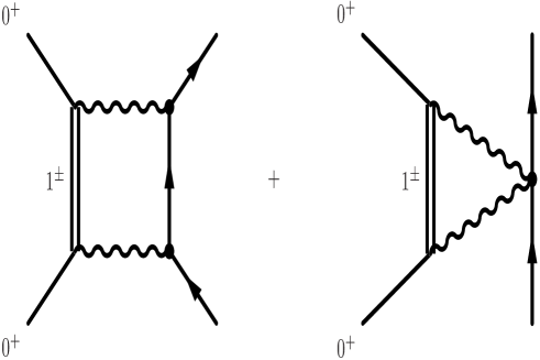
Figure 2: One loop diagrams used to model the interaction of a charged particle with a neutral polarizable system.

There exist additional examples—a similar result obtains by considering the generation of an electric quadrupole moment by an external field gradient. Defining the field gradient via

$$E_{ij}={1\over 2}(\nabla_{i}E_{j}+\nabla_{j}E_{i}))$$ (24)

and the quadrupole polarizability via

$$Q_{ij}=4\pi\alpha_{E2}E_{ij}$$ (25)

The classical energy due to interaction of this moment with the field gradient is given by

$$U=-{1\over 2}\alpha_{E2}E_{ij}E_{ij}$$ (26)

The quadrupole polarizability can be modelled in terms of excitation to a $J^{P}=2^{+}$ excited state and again, a simple one loop calculation finds a combination of classical and quantum terms. Similarly, in a gravitational analog, the presence of a point mass produces a field gradient which generates a gravitational quadrupole, which in turn interacts with the field gradient and leads to a classical energy.

Finally, the gravitational potential between two heavy masses has been treated to one loop in an effective field theory treatment of quantum gravity[8]. Again, the diagrams involving two graviton propagators in a loop yield square root nonanalytic terms which reproduce the nonlinear classical corrections to the potential which are predicted by general relativity[9]. This feature has been known for some time[10].

5 A dispersive treatment

The lesson here is clear—these examples all involve one loop diagrams which contain a combination of classical and quantum mechanical effects, wherein the classical piece is signaled by the presence of a square root nonanalyticity while the quantum component is associated with a $\ln-q^{2}$ term. These results violate the usual expectation of the loop-$\hbar$ expansion. We can further understand the association of classical effects with massless particles by studying a dispersive treatment. In this approach we can see directly that the classical terms are associated with the dispersion integral extending down to zero momentum, which is possible only if the particles in the associated cut are massless.

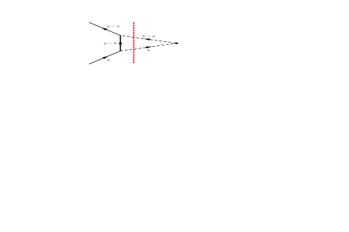
Figure 3: Generic triangle diagram used in dispersive analysis.

It is useful to use the Cutkosky rules to look at the absorptive component of the triangle diagram shown in Figure 3, wherein we assume (temporarily) that the exchanged particles have mass $\mu$. A simple calculation yields[11]

$$\gamma(q^{2})\equiv{\rm Abs}\int{d^{4}k\over(2\pi)^{4}}{1\over(k^{2}-\mu^{2})((k-q)^{2}-\mu^{2})((k-p)^{2}-M^{2})}$$ (27)

$$= \int{d^{4}k\over(2\pi)^{4}}{(2\pi i)^{2}\delta(k^{2}-\mu^{2})\delta((k-q)^{2}-\mu^{2})\over(k^{2}-\mu^{2})((k-q)^{2}-\mu^{2})((k-p)^{2}-M^{2})}$$

where

$$\gamma(q^{2})={1\over 8\pi\sqrt{q^{2}(4M^{2}-q^{2})}}{\rm tan}^{-1}{\sqrt{(q^{2}-4\mu^{2})(4M^{2}-q^{2})}\over q^{2}-2\mu^{2}}$$ (28)

The corresponding dispersion integral is given by

$$\Gamma(q^{2})={1\over\pi}\int_{4\mu^{2}}^{\infty}{dt\gamma(t)\over t-q^{2}-i\epsilon}$$ (29)

The argument of the arctangent vanishes at threshold and the dispersion integral yields a form of no particular interest. On the other hand in the limit $\mu\rightarrow 0$, the argument of the arctangent becomes infinite at threshold and instead we write

$$\gamma(q^{2})={1\over 8\pi\sqrt{q^{2}(4M^{2}-q^{2})}}\left[{\pi\over 2}-{\rm tan}^{-1}\sqrt{q^{2}\over(4M^{2}-q^{2})}\right]$$ (30)

where we have separated the result into two components—the piece proportional to $\pi/2$, which arises from the on-shell (delta function) piece of the mass M propagator and the remaining terms which arise from the principal value integration. The dispersion integral now begins at zero and yields a logarithmic result from pieces of $\gamma(q^{2})$ which behave as a constant as $q^{2}\rightarrow 0$, while square root pieces arise from terms in $\gamma(q^{2})$ which behave as $1/\sqrt{q^{2}}$ in the infrared limit. From Eq. 30 we see that the former—the quantum component—arises from the principal value integration while the latter—the classical component—is associated with the on- shell contributions to $\gamma(q^{2})$. This is to be expected. A classical contribution should arise from the case where both initial/final and intermediate state particles are on shell and therefore physical.

In the electromagnetic case, we can understand how such a classical term arises by writing the Maxwell equation as

$$A_{\mu}={1\over\Box}j_{\mu}$$

Since the inverse D’Alembertian corresponds to the photon propagator, we see that components of the triangle integral involving the massive particle being on-shell leads to physical values of the charge density $j_{\mu}$ and therefore to physical values of the vector potential. Comparing with Eqn. 28 we see that if $\mu\neq 0$ then, there exists no possibility of a square root term and therefore no way for classical physics to arise. Thus the existence of classical pieces can be traced to the existence of two (or more!) massless propagators in the Feynman integration.

6 Conclusions

We have seen above that in the presence of at least two massless propagators, classical physics can arise from loop contributions, in apparent contradiction to the usual loop- $\hbar$ expansion arguments. The presence of classical corrections are associated with a specific nonanalytic term in momentum space. Using a dispersion integral the origin of this phenomenon has been traced to the infrared behavior of the Feynman diagrams involved, which is altered dramatically when the threshold of the dispersion integration is allowed to vanish, as can occur when two or more massless propagators are present. We conclude that the standard expectation that the loop expansion is equivalent to an $\hbar$ expansion is not valid in the presence of coupling to two or more massless particles.

Acknowledgements

We thank A. Zee for comments on the manuscript. This work was supported in part by the National Science Foundation under award PHY-02-44802.

References

-
[1]
See, e.g., R.J. Rivers, Path
Integral Methods in Quantum Field Theory, Cambridge Univ. Press, New York (1987),
sec. 4.6,
L. H. Ryder, Quantum Field Theory, Cambridge Univ. Press, New York (1985), p. 327,
C. Itzykson and J.-B. Zuber, Quantum Field Theory, McGraw Hill, New York (1980), sec. 6-2-1. - [2] J.F. Donoghue, B.R. Holstein, B. Garbrecht, and T. Konstandin, “Quantum corrections to the Reissner-Nordstroem and Kerr-Newman metrics,” Phys. Lett. B529, 132 (2002) [arXiv:hep-th/0112237].
- [3] J.D. Jackson, Classical Electrodynamics, Wiley, New York (1962).
- [4] N.E.J. Bjerrum-Bohr, J.F. Donoghue, and B.R. Holstein, ‘Quantum corrections to the Schwarzschild and Kerr metrics,” Phys. Rev. D68, 084005 (2003) [arXivhep-th/0211071].
- [5] S. Weinberg, Gravitation and Cosmology, Wiley, New York (1972).
- [6] J. Bernabeu and R. Tarrach, “Long Range Potentials And The Electromagnetic Polarizabilities,” Ann. Phys. (NY) 102, 323 (1976).
- [7] G. Feinberg and J. Sucher, Phys. Rev. A27, 1958 (1983).
- [8] N. E. J. Bjerrum-Bohr, J. F. Donoghue and B. R. Holstein, ‘Quantum gravitational corrections to the nonrelativistic scattering potential of two masses,” Phys. Rev. D67, 084033 (2003) [arXiv:hep-th/0211072].
-
[9]
J. F. Donoghue,“General Relativity As An Effective Field Theory: The Leading
Quantum Corrections,”
Phys. Rev. D50, 3874 (1994) [arXiv:gr-qc/9405057].
I. B. Khriplovich and G. G. Kirilin, arXiv:gr-qc/0402018 and JETP 95, 981 (2002) [arXiv:0207118]. -
[10]
S. N. Gupta and S. F. Radford, ‘Quantum Field Theoretical Electromagnetic And
Gravitational Two Particle Potentials,”
Phys. Rev. D21, 2213 (1980).
D. G. Boulware and S. Deser, ‘Classical General Relativity Derived From Quantum Gravity,” Ann. Phys. (NY) 89, 193 (1975). - [11] S. Scherer, Adv. Nucl. Phys. 27, 277 (2003). [arXiv hep-ph/0210398].