Lab/UFR-HEP0403/GNPHE/0403/IFTCSIC/0422
RG Cascades in Hyperbolic Quiver Gauge Theories

Abstract

In this paper, we provide a general classification of supersymmeric QFT₄s into three basic sets: ordinary, affine and indefinite classes. The last class, which has not been enough explored in literature, is shown to share most of properties of ordinary and affine super QFT₄s. This includes, amongst others, its embedding in type II string on local Calabi-Yau threefolds. We give realizations of these supersymmetric QFT₄s as D-brane world volume gauge theories. A special interest is devoted to hyperbolic subset for its peculiar features and for the role it plays in type IIB background with non zero axion. We also study RG flows and duality cascades in case of hyperbolic quiver theories. Comments regarding the full indefinite sector are made.

Keywords: Indefinite Lie algebras, Super Quiver Gauge Theories, Type IIB strings, Hyperbolic gauge model, Cascades and Dualities, Weyl Transformations.

1 Introduction

The study of 4D supersymmetric quiver ADE gauge theories and their affine extensions has attracted a lot of attention in the last few years. In fact, this interest is mainly due to their specific realization as D-brane world volume gauge theories [1] and also to the role they play in low energy type II superstring compactifcations [2]-[5]. Supersymmetric quiver gauge theories were at the basis in deriving Dijkgraaf-Vafa (DV) theory [6]-[8] and generally in the study of large N duality and geometric transitions [9] in type II string compactification on Calabi-Yau threefolds (CY3) with ADE geometries [10]-[12].

One of the objectives of the present study is to extend results of 4D $\mathcal{N}$$=2$ and $\mathcal{N}$$=1$ ordinary and affine ADE quiver gauge models to more general supersymmetric gauge theories. The new class we will consider here, which we dub indefinite class, concerns those 4D super QFTs that are associated with the indefinite sector of simply laced Lie algebras [13]-[15]. Like for affine ADE models with their special properties such as super-conformal invariance and RG cascades [16]-[19], these new quiver gauge theories exhibit as well very remarkable features despite they are not conformally invariant [20]. They appear as low energy field theory limit of type II strings on CY3 with indefinite geometries and have D-brane realizations quite similar to those realizing affine models. Throughout this study, we also complete the picture on 4D supersymmetric quiver gauge theories that may be embedded in type IIB string compactified on more general local CY3s. In particular, we show that indefinite symmetries have remarkably a special hyperbolic sub-invariance which:
(1) serves as a laboratory to explore the indefinite class of quiver gauge theories,
(2) push a step further Fiol analysis [27] extending Klebanov-Strassler affine A${}_{1}^{2}$ model [17, 18] and,
(3) appears, surprisingly, as a symmetry in type IIB background with non zero axion.
The last property gives an explicit evidence for the role played by hyperbolic invariance in type IIB string theory and opens an issue to look for hidden symmetries in string theory. We also study field dualities in hyperbolic model and show that, like in affine case, these theories have duality cascades.

The presentation of this work is as follows. In section 2, we give general features on indefinite quiver gauge theories; in particular on the special hyperbolic subset; its roots system and hyperbolic Weyl group. We show that these objects play a key role in the geometric engineering of hyperbolic quiver QFT₄s and their duals. In section 3, we develop the general setting of indefinite 4D quiver gauge theories embedded in type IIB strings on Calabi-Yau threefolds. Particular interest is given to the hyperbolic subset. In section 4, we study the RG flows for hyperbolic theories and analyze there duality cascades. Section 5 is devoted to summarize our findings and to make an outlook. Two appendices on indefinite Lie algebras and hyperbolic ADE quiver gauge models are given in section 6.

2 Indefinite quiver gauge theories

In this section we want to extend results of four dimensional supersymmetric ADE quiver gauge theories and their affine extensions to other supersymmetric gauge models with more general symmetries. To begin, note that as far as $\mathcal{N}=2$ supersymmetric QFT₄s are concerned, one immediately realizes that affine quiver gauge theories are not the unique possible generalization of ordinary ADE QFT₄s. There are infinitely many others that may be constructed, these concern the class of indefinite quiver gauge theories that interests us here. A more interesting thing in this issue is that the mysterious indefinite set contains the subset of hyperbolic gauge models which have the property of being closer to the standard affine Kac-Moody (KM) models.

In what follows, we give a classification theorem of all possible 4D supersymmetric $\Pi_{i}U\left(N_{i}\right)$ quiver gauge theories. This theorem allows us to have a full picture on 4D super-quiver field models and opens a window on the role of indefinite Lie symmetries in field and string theories. We will mainly focus on 4D $\mathcal{N}=2$ quiver gauge models to elaborate the results, but by switching on non linear adjoint matter self interactions, one gets the corresponding $\mathcal{N}=1$ ones.

2.1 Classification of Super QFT₄s

In classifying 4D supersymmetric quiver gauge theories, we use two standard results:

(1) the field theoretical correspondence between Dynkin diagrams $\mathcal{D}\left(g\right)$ of Lie algebras $g$ on one hand and matter and gauge content in 4D supersymmetric quiver gauge theories on the other hand [10]. This correspondence is defined by associating to each diagram $\mathcal{D}\left(g\right)$ of a ( simply laced ) Lie algebra, a quiver SQFT₄,

$$\mathcal{D}\left(g\right)\mathcal{\qquad\longleftrightarrow\qquad}\text{Super-QFT}_{4}.$$ (2.1)

This means that degrees of freedom in supersymmetric quiver QFT₄ are completely encoded in the graph $\mathcal{D}\left(g\right)$. In $\mathcal{N}=1$ superspace language, the explicit rule is as follows: (a) The i-th node of $\mathcal{D}\left(g\right)$ encodes a gauge multiplet $V_{i}$ and a chiral matter $\Phi_{i}$ superfield both transforming in the adjoint representation of $U\left(N_{i}\right)$. (b) Links $\left|K_{ij}^{q}\right|$ between i-th and j-th nodes of $\mathcal{D}\left(g\right)$ give the number of bi-fundamental matter chiral multiplets $Q_{ij}\oplus Q_{ji}$ transforming in $\left(N_{i},\overline{N}_{j}\right)$ representation of $U\left(N_{i}\right)\times U\left(N_{j}\right)$.

(2) Classification of possible Dynkin diagrams $\mathcal{D}\left(g\right)$ of Lie algebras. This classification is given by two fundamental Lie algebraic theorems: (a) Vinberg theorem [21] asserting that in general there are three basic subsets of Dynkin diagrams which, for convenience, we denote them as,

$$\mathcal{D}^{+}\left(g\right)\text{;\qquad}\mathcal{D}^{0}\left(g\right)\text{;\qquad}\mathcal{D}^{-}\left(g\right).$$ (2.2)

These are respectively associated with finite dimensional Lie algebras, affine KM extension and indefinite generalization. (b) Cartan type classifications [22, 23] of above Dynkin diagrams eq(2.2) encoded in the following statement (i) The usual Cartan classification of Dynkin diagrams $\mathcal{D}^{+}\left(g\right)$,

$$\mathcal{D}^{+}\left(A_{r}\right),\qquad\mathcal{D}^{+}\left(D_{r}\right),\qquad\mathcal{D}^{+}\left(E_{6,7,8}\right),$$ (2.3)

where A_r, D_r and E_r are the usual rank $r$ simply laced finite dimensional Lie algebras. (ii) KM classification of affine Lie algebras with co-rank one graphs $\mathcal{D}^{0}\left(g\right)$,

$$\mathcal{D}^{0}\left(\widehat{A}_{r}\right),\qquad\mathcal{D}^{0}\left(\widehat{D}_{r}\right),\qquad\mathcal{D}^{0}\left(\widehat{E}_{6,7,8}\right),$$ (2.4)

where $\widehat{A}$ stands for the affine extension of $A$ and so on. (iii) For the classification of Dynkin diagrams $\mathcal{D}^{-}\left(g\right)$ of indefinite simply laced Lie algebras, there have been many attempts but unfortunately with partial results only since a complete classification does not exist yet. However, there is an interesting partial classification which can be used to approach the indefinite sector. This partial classification [24, 14], which will be considered in the present study, deals with the W. Li hyperbolic Dynkin diagrams denoted as $\mathcal{D}^{-}\left(H_{r}^{s}\right)$ where r and s are integers. Results in this matter are reported in appendix A, for a general analysis and other conventional notations see [24, 25].

2.2 Theorem

As far as Dynkin graphs of simply laced Lie algebras are concerned, there are three kinds of four dimensional supersymmetric quiver gauge theories:

(1) The usual four dimensional supersymmetric ordinary ADE quiver gauge theories. Their content in gauge and matter super multiplets are encoded by the ordinary simply laced ADE Dynkin diagrams according to the rule given above. These theories are not scale invariant, they appear as type II strings low energy limits and have realization as gauge theories in the world volume of partially wrapped D-branes.

(2) The well common supersymmetric affine $ADE$ quiver gauge theories which can be viewed as the simplest extension of the previous ones. They are obtained by adding more gauge and matter multiplets according to the structure of affine $ADE$ Dynkin diagrams. These supersymmetric quantum field models are specific gauge theories, they may be conformal and have a remarkable realization as D3-brane world volume gauge theories.

(3) An indefinite sector of supersymmetric quiver QFT₄s. These gauge theories have not been enough explored in the literature, they can be thought of as given by the set of all remaining possible generalizations of ordinary quiver gauge theories except affine KM extensions. Indefinite quiver gauge theories include the hyperbolic quiver gauge models as a special subset.

2.3 Supersymmetric Action

From the classification above, we deduce that given a Cartan matrix $K^{q}\left(g\right)$ and Dynkin diagram $\mathcal{D}^{q}\left(g\right)$, with $q=1,0,-1$ referring respectively to ordinary simply laced Lie algebras, affine KM extension and indefinite generalization, one can determine the appropriate number of propagating degrees of freedom of the corresponding supersymmetric quiver QFT₄. The rule is as follows [5]: To the i-th node of $\mathcal{D}^{q}$, one associates a gauge multiplet $V_{i}$ and a chiral matter one $\Phi_{i}$ transforming in adjoint representation of $U\left(N_{i}\right)$. For $\left|K_{ij}^{q}\right|$ ($K_{ij}^{q}=0,-1$ for present case), links between i-th and j-th nodes of $\mathcal{D}^{q}$, one associates bi-fundamental matter $Q_{ij}$ transforming in $\left(N_{i},\overline{N}_{j}\right)$ representation of $U\left(N_{i}\right)\times U\left(N_{j}\right)$. With these superfield degrees of freedom, we can write down the general supersymmetric action describing their classical dynamics. In the $N=1$ formalism, the general superfield action $\mathcal{S}_{q}$ reads as:

$$\mathcal{S}_{q} = \int d^{4}xd^{4}\theta\left[\sum_{i,j}Tr\left(Q_{ij}^{\ast}\left[\exp\left(K_{ij}^{q}V_{j}\right)\right]Q_{ji}\right)\right]+\sum_{i}\zeta_{i}\int d^{4}xd^{4}\theta Tr\left(V_{i}\right)$$

$$+\left(\int d^{4}xd^{2}\theta\left[\sum_{i,j}G_{\left[ij\right]}^{q}\lambda_{ij}Tr\left(Q_{ij}\Phi_{j}Q_{ji}\right)+\sum_{i}Tr\left[\mathrm{W}\left(\Phi_{i}\right)\right]\right]+hc\right)$$

$$+\left(\int d^{4}xd^{2}\theta\left[\sum_{i}Tr\left(\Phi_{i}^{\ast}e^{K_{ii}^{q}adV_{i}}\Phi_{i}\right)\right]+\int d^{4}xd^{2}\theta\left[\sum_{i}\frac{1}{g_{i}^{2}}Tr\left(W_{\alpha}^{i}W_{i}^{\alpha}\right)\right]+hc\right),$$

where $W_{i}^{\alpha}$ stand for the spinor gauge field strength. The constants $g_{i}$, $\zeta_{i}$, $\lambda_{ij}$ as well as those contained in $\mathrm{W}\left(\Phi_{i}\right)$, which is a polynomial in adjoint matter ($\mathrm{W}=\sum z_{i}\Phi_{i}+m_{i}\Phi_{i}^{2}...$), are the usual bare coupling constants. Obviously $\mathcal{N}=2$ supersymmetry requires linear adjoint matter superpotentials; i.e $\mathrm{W}=\sum z_{i}\Phi_{i}$, otherwise it is broken down to $\mathcal{N}=1$. Note that the $z_{i}$s should be compared with the FI coupling $\zeta_{i}$; they will play a crucial role in next sections when we study Seiberg like field duality. Note also that since Cartan matrices of simply laced Lie algebras are symmetric, they can be expressed in terms of the $T_{ij}^{q}$ triangle matrices ($i\geq j$) and their transpose $T_{ji}^{q}$ as $K_{ij}^{q}=T_{ij}^{q}+T_{ji}^{q}$. These $T_{ij}^{q}$s are also used in writing the $G_{\left[ij\right]}^{q}$ antisymmetric matrices appearing in above relation as $G_{[ij]}^{q}=T_{ij}^{q}-T_{ji}^{q}$. Finally, observe that the above quiver gauge theory has an interpretation in type IIB string theory as world volume theories on regular D3-branes and partially wrapped D5 ones. We will turn to this representation later when we consider the brane realization of hyperbolic gauge theories. From the action above, one can determine the superfield eqs of motion. For the matter’s case and up on dropping kinetic terms non sensitive to complex deformations, we obtain the following superfield equations of motion,

$$Q_{ij}Q_{ji}-Q_{ji}Q_{ij} = W_{i}^{{}^{\prime}},$$

$$Q_{ij}\Phi_{j} = \Phi_{i}Q_{ij}.$$ (2.6)

For linear superpotential $W$, these eqs describe, for each gauge group factor, an $O(-2)\oplus O(0)$ Calabi-Yau threefold and the quiver gauge theory has $\mathcal{N}=2$ supersymmetry. For generic polynoms in $\Phi_{i}$s however, $\mathcal{N}=2$ supersymmetry is explicitly broken down to $\mathcal{N}=1$. The new geometry of the Calabi-Yau threefolds associated with each gauge group factor is now $O(-1)\oplus O(-1)\rightarrow P^{1}$. Following DV theory, this manifold may undergo a geometric transition where the blow down $S^{2}$ spheres are replaced by $S^{3}$ and the partially wrapped D5-branes by three form fluxes. At this level nothing requires a distinction between indefinite quiver gauge theories and the ordinary and affine ones. This property let understand that basic results on the familiar supersymmetric quiver gauge theories are also valid for the indefinite case. Therefore like for ordinary and affine ADE quiver gauge models which are known as QFT limits of type II string on CY3 with ordinary and elliptic ADE singularities respectively, it is natural to think about the indefinite quiver gauge theories defined above as also following from type II string compactification on CY3 with indefinite singularities. The structure of these indefinite singularities and the underlying singularity theory is still an open question; but we fortunately dispose of some explicit examples realizing CY3 manifolds with indefinite singular CY3s. For details on this issue; we refer to [15, 16].

3 Hyperbolic Quiver Gauge models

Hyperbolic quiver gauge models constitute a special subset of indefinite quiver gauge theories that are based on hyperbolic Lie algebras. Some of these hyperbolic models may be also viewed as simplest extension of the usual supersymmetric affine ADE theories. Moreover, they can be also obtained as low energy limit of type IIB string on CY3s with hyperbolic singularities and have a realization as D-brane world volume gauge theories. In order to show how these special supersymmetric theories are built, we first review some useful properties on hyperbolic Lie algebras as well as their algebraic geometry analog. Then, we consider their realization as world volume gauge theories of D-branes wrapping cycles in CY3s with hyperbolic geometries.

3.1 Roots and Homology in Hyperbolic ADE Geometries

Roughly speaking, there are two main classes of hyperbolic simply laced Lie algebras: standard hyperbolic algebras and the so called strictly hyperbolic ones. For precise definitions on these two varieties of indefinite Lie algebras see [25],[26],[15]. In this paper we will be interested in standard hyperbolic algebras, they can be thought of as particular extension of affine simply laced Kac-Moody invariance. Note that the hyperbolic symmetries we will be considering here are very special, we will refer to them as hyperbolic ADE algebras, a matter of keeping in mind that these symmetries contain the usual finite ADE Lie algebras and their affine analog as Lie subalgebras.

Roots and cycles in hyperbolic model

Since hyperbolic ADE Lie algebras are simplest extensions of affine KM ones, one can easily make an idea on this larger structure. More precisely, basic tools of these hyperbolic ADE Lie algebras are quite same as those used in affine KM symmetries. Of course there are also novelties, but these can be extracted by using similarity arguments to be specified later on. Let comment briefly how these hyperbolic ADE algebras can be obtained from the underlying affine ones; for a rigorous derivation and details see [21].

Simple roots:  Starting from a rank r affine simply laced Kac-Moody algebra with the usual simple roots $\alpha_{i},$ with $i=0,1,...,r$ where $\alpha_{0}=\delta-\sum_{i=1}^{r}d_{i}\alpha_{i}$ with $\delta$ being the usual imaginary root and the other $\alpha_{i}$s the simple real ones, we can write down several relations for hyperbolic ADE Lie algebras just by using intuition and similarity arguments. The rule is as follows: Once an affine ADE Cartan matrix $K_{ij}^{0}=\alpha_{i}.\alpha_{j}$ and corresponding Dynkin diagram $\mathcal{D}^{0}$ are fixed, a hyperbolic ADE generalization of Cartan matrix and Dynkin graph are obtained by adding an extra simple root $\alpha_{-1}$ to the game with the property,

$$\alpha_{-1}.\alpha_{-1}=2;\qquad\alpha_{-1}\alpha_{0}=-1;\qquad\alpha_{-1}\alpha_{i}=0.$$ (3.1)

It happens that, because of the Lorentzian nature of the root lattice of hyperbolic ADE algebras, this extra simple root is realized in a different manner comparing to what we do in ordinary and affine cases. In addition to standard simple roots $\alpha_{i}$, with $i=0,1,...,r$, we have,

$$\alpha_{-1}=\gamma-\delta;\qquad\gamma^{2}-2\gamma.\delta+\delta^{2}=2,$$ (3.2)

with $\gamma$ a second basic imaginary root related to the standard imaginary root $\delta$ of affine KM as well as to the previous real simple roots $\alpha_{i}$ of finite subalgebra as follows,

$${\gamma}^{2} = {\delta}^{2}=0;\qquad{\gamma}{\delta}=-1,$$

$${\gamma.}\alpha_{0} = 1;\qquad{\gamma.}\alpha_{i}=0,\ i>0.$$ (3.3)

Therefore our hyperbolic ADE Lie algebras have two basic imaginary roots $\gamma$ and $\delta$ which a priori should play a completely symmetric role. This property will be one of the main arguments that allow us to extract part of remaining information on the hyperbolic ADE structure that are not captured by affine KM subsymmetry.  Note that the symmetric role between $\gamma$ and $\delta$ is not hazardous; but it reflects invariance of hyperbolic root system under Weyl transformations. For details we refer to the above mentioned paper.

Cycles:  In the present study we are also interested in type IIB string interpretation on CY3s of the 4D supersymmetric quiver gauge theories based on the Dynkin diagrams of hyperbolic algebras. It is then interesting to find a geometric meaning of the $\gamma$ and $\delta$ imaginary roots in homology of CY3s with hyperbolic ADE geometry. Formal analogy with affine models shows that $\gamma$ and $\delta$ should correspond to two homological two cycles of CY3s. Extending results on type II string interpretation of affine models to the hyperbolic ADE case, we see that geometrically speaking, $\gamma$ and $\delta$ generate a two torus; or more precisely two heterotic torii $T_{\pm}^{2}$. The latters may be thought of as holomorphic T${}_{z}^{2}$ and anti-holomorphic T${}_{\overline{z}}^{2}$ two cycles in Kahler threefolds. This observation constitutes a key point in our analysis of hyperbolic ADE quiver gauge models. It allows us to construct the complex two dimension homology of the needed CY3s.

In what follows, we build the explicit root system of hyperbolic ADE Lie algebras without using involved technical details. The corresponding hyperbolic algebraic geometry is recovered by using the standard dictionary on this matter relating Lie algebra roots and algebraic geometry corresponding quantities.

Hyperbolic root system

As noted before, the $\gamma$ and $\delta$ imaginary roots allow us to get many precious informations not only on hyperbolic Lie algebra, but also on corresponding algebraic geometry analog. We focus our attention on the derivation of the root system of hyperbolic ADE Lie algebras from which we directly determine the corresponding CY3s homological cycles. To that purpose, note that from construction the imaginary roots $\gamma$ and $\delta$ play a completely symmetric role. This symmetric property, which corresponds to a Weyl rotation, turns out to have important implications on the construction of hyperbolic ADE root system, the derivation H₂ homology classes of the CY3 with hyperbolic geometry and on the study of hyperbolic quiver gauge theories. One of these implications follows from the fact that as roots, $\gamma$ and $\delta$ can be usually expanded in terms of the simple roots $\left\{\alpha_{i};-1\leq i\leq r\right\}$ of the hyperbolic algebra as,

$$\delta=\sum_{i=0}^{r}d_{i}\alpha_{i};\qquad\gamma=\sum_{i=-1}^{r}d_{i}\alpha_{i},$$ (3.4)

where $d_{i}$, $0\leq i\leq r$ are the usual Dynkin weights and where $d_{-1}$, which is equal to one, is their analog for the hyperbolic node. In the present study, we will think about all these $d_{i}$s ( $-1\leq i\leq r$) as generic positive integers and treat them on equal footing. While in affine KM symmetries, $\delta=\sum_{i=0}^{r}d_{i}\alpha_{i}$ is a standard relation, $\gamma=\sum_{i=-1}^{r}d_{i}\alpha_{i}$ is a specific one for the hyperbolic case. Note that upon setting $d_{0}=0$ in the expansion of $\gamma$, we see that $\gamma^{\ast}=\gamma|_{d_{0}=0}$ can play perfectly the role of a KM imaginary root in the same manner as does $\delta$. A way to see this property is to rename the $\alpha_{-1}$simple root as $\alpha_{-1}|_{d_{0}=0}=\alpha_{0}^{\ast}$ and notes that the restriction ( projection) $\delta|_{d_{0}=0}$ is just the maximal root $\psi$ of the usual underlying finite dimensional Lie algebra. Moreover in homology language the above relations correspond to the two cycles,

$$T_{+}^{2}=\sum_{i=0}^{r}d_{i}S_{i}^{2};\qquad T_{-}^{2}=\sum_{i=-1}^{r}d_{i}S_{i}^{2},$$ (3.5)

where naively the $S_{i}^{2}$s are the usual real two spheres of type II strings on CY3s with deformed ADE singularities. Using results of affine KM invariance and the symmetric role between $\gamma$ and $\delta$, we can derive the hyperbolic root ( two cycles) system $\Delta_{hyp}$ (in CY3s). Following [21], the full set $\Delta_{hyp}$ of roots of hyperbolic Lie algebras is as follows,

$$\Delta_{hyp}\cup\{0\}=\{a=n\gamma+m\delta+l\alpha;n,m\in Z;l=0,\pm 1;\alpha\in\Delta_{finite}\},$$ (3.6)

where $\Delta_{finite}$ stands for the roots system of finite dimensional ADE Lie sub-algebras. A rigorous way to get the system $\Delta_{hyp}$ is to solve constraint eqs required by the hyperbolic structure [21]. Nevertheless, there is also short path to get this result. The idea, which is done in two steps, is as follows:

(1) Observe that our hyperbolic Lie algebra $g_{hyp}$ has remarkably two special affine Kac-Moody sub-algebras $g_{aff}^{\gamma}$ and $g_{aff}^{\delta}$ in one to one correspondence with the two imaginary roots $\gamma$ and $\delta$ encountered above. So root system $\Delta_{hyp}$ should contain as subsystems $\Delta_{aff}^{\gamma}$ and $\Delta_{aff}^{\delta}$ respectively generated by $\gamma$ and $\delta$. This is clearly seen on above relation from which it is not difficult to see that the root systems of $g_{aff}^{\gamma}$ and $g_{aff}^{\delta}$ are respectively given by,

$$\Delta_{aff}^{\gamma}\cup\{0\} = \{a=n\gamma+l\alpha;n\in Z;l=0,\pm 1;\alpha\in\Delta_{finite}\},$$

$$\Delta_{aff}^{\delta}\cup\{0\} = \{a=m\delta+l\alpha;m\in Z;l=0,\pm 1;\alpha\in\Delta_{finite}\},$$ (3.7)

where $\gamma$ and $\delta$ play the role of the basic imaginary root in each sector.

(2) Think about hyperbolic Lie algebra just as an interpolation between these two affine sub-symmetries where roots $n\gamma+m\delta+l\alpha$ are between $n\gamma+l\alpha$ and $m\delta+l\alpha$ recovered by solving the constraint eq $nm=0$. The special case $m=n=0$ corresponds just to root system of underlying finite dimensional ADE. This way of doing can be also used to derive Weyl group $W_{hyp}$, it is given by $W_{finite}\ltimes T$; i.e the semi-direct product of ordinary Weyl group $W_{finite}$ with the group of translations $T$ in the hyperbolic co-root lattice.

3.2 Hyperbolic gauge model

As already noted, hyperbolic quiver gauge theories can be thought of as the simplest extension of supersymmetric affine ADE ones. All what we know on affine quiver gauge models can be extended to the hyperbolic case. Let us consider the extension of those quantities that are relevant for the present study by using the similarity argument.

To make a parallel between hyperbolic and affine supersymmetric quiver theories as well as their type II string interpretations, one has to answer a basic question regarding string coupling $g_{s}$. As we know, this coupling is strongly linked with the imaginary root $\delta$ ( two torus) of the deformed elliptic singularity of CY3 on which type II string is compactified. In hyperbolic quiver gauge models, one has two fundamental imaginary roots $\gamma$ and $\delta$ ( two heterotic torii) and so one should expect two kinds of basic moduli. This is not a problem in type IIB string since we have two candidates for these moduli namely the dilaton field $\phi$ and the RR axion $\chi$. In addition to type II string compactification on CY3s with elliptic singularities, we see that we also have solutions involving CY3 folds with hyperbolic singularities. A way to motivate this class of backgrounds is to note that the usual type IIB string coupling constant,

$$g_{s}=exp\phi,$$ (3.8)

can be usually promoted to $g_{\pm}$ by considering non zero values for the RR axion field $\chi$. This may be done by mimicking the construction used in the derivation of F-theory. The idea consists to shift string coupling $g_{s}$ as follows,

$$g_{s}^{-1}=exp(-\phi)\qquad\rightarrow\qquad g_{\pm}^{-1}=exp(-\phi)\pm\chi,$$ (3.9)

but still keeping reality condition. This leads however to an indefinite product $g_{+}g_{-}$ since the quantity $g_{+}^{-1}g_{-}^{-1}=g_{s}^{-2}-\chi^{2}$ has a Lorentzian signature. Upon performing a Wick rotation of the RR axion moduli ($\chi\longrightarrow i\chi$), the inverse string coupling $g_{+}^{-1}$ becomes $g_{\tau}^{-1}=exp(-\phi)-i\chi$ which should be compared with the complex moduli $i\tau_{IIB}$ of the holomorphic two torus used in F-theory compactification on elliptic K3 [26]. The other coupling $g_{-}^{-1}$ becomes $g_{\overline{\tau}}^{-1}=exp(\phi)+i\chi$ and should be associated with the complex moduli $-i\bar{\tau}_{IIB}$ of the anti-holomorphic torus obtained by taking complex conjugation. Moreover demanding positivity of the $g_{\pm}$ couplings constants oblige the range of $\phi$ and $\chi$ moduli to satisfy a constraint. Taking the dilaton as the basic modulus with an arbitrary real value, the range of the axion RR field should like,

$$\left|\chi\right|\leq exp(-\phi).$$ (3.10)

To get the relation between $g_{\pm}$ and the $g_{i}$ moduli of the hyperbolic quiver gauge theory, it is enough to recall the relation between the string coupling $g_{s}$ and the $g_{i}$ gauge couplings in the affine model.

$$g_{s}^{-1}=\sum_{i=0}^{r}d_{i}g_{i}^{-2},$$ (3.11)

where $d_{i}$s are the Dynkin weight encountered above. This relation can be viewed as just corresponding to the special case of a zero axion field. For the general case where there is a non zero axion, we have two couplings $g_{\pm}$ and so the previous relation generalizes as follows:

$$g_{-}^{-1}=\sum_{i=0}^{r}d_{i}g_{i}^{-2};\qquad g_{+}^{-1}=\sum_{i=-1}^{r}d_{i}g_{i}^{-2};$$ (3.12)

where $g_{-1}$ is the gauge coupling of the gauge group engineered on the hyperbolic node of the Dynkin diagram $\mathcal{D}^{-}$. From above relation, we also see that the parameters $g_{\pm}$ are linked as follows,

$$g_{+}^{-1}=g_{-1}^{-2}+g_{-}^{-1},$$ (3.13)

Substituting $g_{+}^{-1}$ and $g_{-}^{-1}$ by the dilaton and the axion expressions, we get $g_{-1}^{-2}=2\chi$. This show that the RR axion field is identified with the volume of the hyperbolic node in the hyperbolic ADE geometry. Taking $\chi=0$, one recovers the usual affine model with all desired features.

3.3 Brane realization

A way to get the D-brane realization of hyperbolic ADE gauge theories living in D-brane world volume is as follows. Start from the usual D-brane representation of the affine ADE quiver gauge model and appropriately deform the gauge system towards the hyperbolic case. This can be done by help of the root system of the hyperbolic ADE algebras and their algebraic geometry analog.

Affine model

To begin recall that in affine ADE model, one has in general $N_{0}$ coincident regular D3-branes and $N=\sum_{i=1}^{r}N_{i}$ fractional D5-branes. Each block of the $r$ sets of $N_{i}$ D5-branes is wrapped over two cycles of the deformed ADE geometry of the local CY3. The homological properties of these $r$ real two cycles can be obtained from the properties of simple roots of ADE Lie algebra. One of these features is that the irreducible components $\mathbb{P}_{i}^{1}$ of the homological chain $\sum_{i}d_{i}\mathbb{P}_{i}^{1}$ are not free but rather glued as follows,

$$C_{\psi}=\sum_{i=1}^{r}d_{i}\mathbb{P}_{i}^{1};\qquad C_{\psi}^{2}=-2;\qquad\mathbb{P}_{i}^{1}.\mathbb{P}_{j}^{1}=-K_{ij}^{+}.$$ (3.14)

In this relation the two cycle $C_{\psi}$ is the open two-chain corresponding to the maximal root $\psi=\sum_{i}d_{i}\alpha_{i}$ of finite ADE Lie algebra. In fact the $C_{\psi}$ chain should be thought of as just a part of the following closed two-chain

$$C_{\delta}=\sum_{i=0}^{r}d_{i}\mathbb{P}_{i}^{1}=C_{0}+C_{\psi};\qquad\mathbb{P}_{i}^{1}.\mathbb{P}_{j}^{1}=-K_{ij}^{0};\qquad C_{\delta}^{2}=0,$$ (3.15)

which is associated with the imaginary root $\delta$ of affine ADE Kac-Moody algebras. In the above eqs, $K_{ij}^{+}$ and $K_{ij}^{0}$ are as before, they stand for the usual ordinary and affine ADE Cartan matrices respectively. From these eqs, it is not difficult to see that $N_{0}$ is the number of regular D-branes filling space time and living on the loop $C_{\delta}$. Therefore the gauge group of the $\mathcal{N}=2$ supersymmetric affine ADE quiver QFT₄ is,

$$\prod_{i=0}^{r}U\left(\widehat{N}_{i}\right)=U\left(N_{0}\right)\times\prod_{i=1}^{r}U\left(N_{i}+d_{i}N_{0}\right)$$ (3.16)

where for convenience we have set the $\widehat{N}_{i}$s ranks as [13],

$$\widehat{N}_{0}=N_{0};\qquad\widehat{N}_{i}=N_{0}d_{i}+N_{i};\qquad 1\leq i\leq r.$$ (3.17)

Knowing the gauge group, one can go ahead and study the quantum dynamics of these supersymmetric quiver gauge theories. Of particular interest is the beta functions $\beta_{i}=\beta\left(g_{i}\right)$ for the gauge couplings $g_{i}$ and the RG flows $\beta_{i}=\beta_{i}\left(\mu\right)$. We will turn to this aspect after giving the brane realization for hyperbolic gauge models.

Hyperbolic Model

In hyperbolic quiver gauge theories extending the previous affine ADE ones, we have also regular coincident D3-branes and fractional D5 ones. But now with a quiver gauge group given by,

$$\prod_{i=-1}^{r}U\left(\widehat{N}_{i}\right)=U\left(N_{-1}\right)\times U\left(N_{0}+d_{0}N_{-1}\right)\times\prod_{i=1}^{r}U\left(N_{i}+d_{i}\left(N_{-1}+N_{0}\right)\right),$$ (3.18)

that is one factor more and an extra stuck of $N_{-1}$ D3-branes. The point is that in case of hyperbolic symmetries, the underlying geometry involves two heterotic torii $C_{\delta}$ and $C_{\gamma}$. The first one is same as the two torus $C_{\delta}$ of eq(3.15), which we call $C^{-}$ and the second is the new closed heterotic chain $C_{\gamma}\equiv C^{+}$ built as,

$$C^{+}=C^{-}+\mathbb{P}_{-1}^{1};\qquad C^{\pm}.C^{\pm}=0;\qquad C^{-}.C^{+}=1.$$ (3.19)

Mimicking the analysis we have done for affine ADE models, we immediately get the D-brane representation of hyperbolic ADE quiver gauge theories. The D-brane system realizing hyperbolic quiver gauge model depends on the sign of the axion modulus and is as follows:

(a) Minimal realization ($\chi<0$):  Besides the previous $N_{0}$ D3-branes on $C^{-}$ and the wrapped $N$ D5 ones ($N=\sum_{i=1}^{r}N_{i}$), we have moreover an extra subset of $N_{-1}$ D3-branes filling the four space time and living on $C^{+}$. These $N_{-1}$ D3-branes capture the hyperbolic extension; and though they look like $N_{0}$ D3-branes from space time view, they carry different internal quantum numbers as they live on a different internal geometry cycle. Therefore D-branes of hyperbolic quiver gauge theories have brane charges $\widehat{N}_{i}$ given by,

$$\widehat{N}_{-1}=N_{-1};\qquad\widehat{N}_{0}=N_{0}+d_{0}N_{-1};\qquad\widehat{N}_{i}=\left(N_{0}+N_{-1}\right)d_{i}+N_{i};\qquad 1\leq i\leq r.$$ (3.20)

These numbers, which can be also read from the algebraic relation (3.4), are direct extension of the affine ADE model considered before. Note that setting $N_{-1}=0$, one recovers the standard affine model and setting $N_{0}=0$ one gets the second supersymmetric quiver CFT₄ hidden in the hyperbolic model; see eqs(3.6-3.7). It would be interesting to deepen the study which link the two critical behaviours inside hyperbolic model.

(b) Non minimal realization ($\chi>0$):  Along with the above representation of the hyperbolic gauge system, we may also have a set of $M_{-1}$ fractional D5-branes wrapping the two cycle

$$C^{-}-C^{+}$$ (3.21)

In this case, eq(3.20) are replaced as

$$\widehat{N}_{-1}=d_{-1}N_{-1}+M_{-1}$$ (3.22)

and the other $\widehat{N}_{i}$ as before. Note that since wrapping D5-branes over two cycles involve positive volumes, non zero $M_{-1}$ requires positive axion moduli, $\chi>0$.

4 RG flows in Hyperbolic model

To fix the ideas, consider the hyperbolic ADE quiver gauge model described by the action (2.3) with all real FI couplings $\zeta_{i}$ set to zero ( $\zeta_{i}=0$). Then focus on linear adjoint matter self-couplings $W\left(\Phi_{i}\right)=z_{i}\Phi_{i}$ so that the gauge theory has $\mathcal{N}=2$ supersymmetry.

4.1 Running couplings

Recall that in the special case where there is no Kahler deformation, the gauge couplings $g_{i}\sim\sqrt{\zeta_{i}^{2}+z_{i}z_{i}^{\ast}}$ of the $\prod_{j=0}^{r}U\left(\widehat{N}_{j}\right)$ symmetry reduce to

$$8\pi^{2}{g_{i}^{-2}}=\left|z_{i}\right|^{2}\geq 0,$$ (4.1)

where $\left|z_{i}\right|=\sqrt{z_{i}z_{i}^{\ast}}$. Since these $z_{i}$s can be varied freely in the moduli space of the hyperbolic quiver QFT₄, the corresponding complex deformations induce variations of the ${g_{i}^{-2}}$s. These variations have a quantum field theoretic interpretation in terms of renormalization group flows ${g_{i}=g_{i}}\left(\mu\right)$. But before going into details, note that for $\zeta_{i}=0$, the real gauge moduli ${g_{i}^{-2}}$ can be usually split as the product of holomorphic factor ${G}{{}_{i}^{-1}}=z_{i}\sqrt{\frac{1}{8\pi^{2}}}$ and its complex conjugate as ${g_{i}^{-2}}={G}{{}_{i}^{-1}}\left({G}{{}_{i}^{-1}}\right)^{\ast}$. This is an expected feature in absence of Kahler deformations; it reflects just holomorphy of complex deformations in $\mathcal{N}=2$ supersymmetric gauge theories. In fact this splitting is not inherent to $\mathcal{N}=2$ supersymmetry; it is also valid for $\mathcal{N}=1$ models for which the previous complex gauge couplings ${G}{{}_{i}}$ generalize as

$${G}{{}_{i}^{-1}}=\frac{1}{2\pi\sqrt{2}}W_{i}^{\prime};\qquad W_{i}^{\prime}=\frac{\partial W}{\partial\Phi_{i}}.$$ (4.2)

Under the change of one or several of the $z_{i}$s in the moduli space of the hyperbolic quiver QFT₄, the corresponding ${g_{i}^{-2}}$ gauge couplings vary too. A physically interesting feature of this change concerns the case where one of the $z_{i}$s vanishes ( ${z}_{i}=0$). In this particular situation, the underlying CY3 geometry in type IIB string compactification becomes singular and the corresponding supersymmetric QFT₄ confine at some gauge scale $\Lambda_{i}$. This property has a quantum field theoretic description in terms of running coupling constants ${g_{i}^{-2}=g_{i}^{-2}}\left(\mu\right)$, which read at ( $\mathcal{N}=2$ exact) one loop as,

$$g_{i}^{-2}\left(\mu\right)=\frac{\beta_{i}}{8\pi^{2}}\ln\left(\frac{\mu}{\Lambda_{i}}\right);\qquad-1\leq i\leq r,$$ (4.3)

where $\beta_{i}=-2\pi\mathrm{i}\beta\left(\tau_{i}\right)$ is the usual holomorphic beta functions with $2\pi\mathrm{i}\tau_{j}=-8\pi^{2}g_{j}^{-2}+\mathrm{i}\vartheta_{j}$ and $\Lambda_{i}$ is the gauge confinement scale we referred to above. Comparing eqs(4.1) and (4.3), we get the following relation between the $z_{i}$ moduli and the running scale $\frac{\mu}{\Lambda_{i}}$,

$$\left|z_{i}\right|=\beta_{i}\ln\left(\frac{\mu}{\Lambda_{i}}\right),$$ (4.4)

linking hyperbolic ADE singularity in the CY3 of the IIB string compactification with the quantum field scale $\mu=\Lambda_{i}$. Note that $\left|z_{i}\right|$ positivity condition, $\left|z_{i}\right|=\beta_{i}\ln\left(\frac{\mu}{\Lambda_{i}}\right)\geq 0$, of the gauge coupling constants can be solved in two ways according to the value of the renormalization scale $\mu$ and the parameter $\Lambda_{i}$. We have:

(a) $\beta_{i}>0$ and $\ln\left(\frac{\mu}{\Lambda_{i}}\right)>0$ which requires $\mu>\Lambda_{i}$, or

(b) $\beta_{i}<0$ and $\ln\left(\frac{\mu}{\Lambda_{i}}\right)<0$ requiring $\mu<\Lambda_{i}$.

The singular limit $\left|z_{i}\right|=0$ corresponds either to $\mu=\Lambda_{i}$ or to $\beta_{i}=0$ independently of the renormalization group scale’s value. At this point, the hyperbolic gauge theory confines and its interpretation as D-branes world volume is sensitive to the sign of the beta functions which we propose to discuss now.

4.2 Holomorphic Beta functions

Following [15], the holomorphic beta function factors $\beta_{i}=\beta\left(g_{i}\right)$ of $\mathcal{N}=2$ supersymmetric $\Pi_{i=-1}^{r}U\left(\widehat{N}_{i}\right)$ quiver gauge theories depend linearly on the $\widehat{N}_{i}$ ranks. They are proportional to the Cartan matrix $K_{hyp}^{-}$ of the underlying hyperbolic quiver symmetry; $\beta_{i}\sim K_{ij}^{-}\widehat{N}_{j}$. For an explicit treatment, we will first consider the particular example of hyperbolic A_r QFT₄. The results for hyperbolic DE cases are given in appendix B.

Hyperbolic A_r model:  In the example of $\mathcal{N}=2$ supersymmetric hyperbolic A_r model, the beta functions for the quiver gauge group can be easily determined. They read as;

$$\beta_{-1} = 2\widehat{N}_{-1}-\widehat{N}_{0};\qquad\beta_{0}=-\widehat{N}_{-1}+2\widehat{N}_{0}-\widehat{N}_{1}-\widehat{N}_{r},$$

$$\beta_{i} = 2\widehat{N}_{i}-\widehat{N}_{i-1}-\widehat{N}_{i+1};\qquad 1\leq i\leq r-1,\qquad\beta_{r}=2\widehat{N}_{r}-\widehat{N}_{r-1}-\widehat{N}_{0}.$$ (4.5)

where $\widehat{N}_{i}$ are as in eq(3.20) and (3.22) according to the sign of the axion modulus.

$(i)$ Minimal representation:  Up on using eqs(3.20) defining the minimal realization of the hyperbolic gauge theory, the previous relations simplify to,

$$\beta_{-1} = N_{-1}-N_{0};\qquad\beta_{0}=-N_{-1}-N_{1}-N_{r};\qquad\beta_{1}=2N_{1}-N_{2},$$

$$\beta_{r} = 2N_{r}-N_{r-1};\qquad\beta_{i}=2N_{i}-N_{i-1}-N_{i+1};\qquad 2\leq i\leq r-1,$$ (4.6)

where one recognizes the usual beta functions for finite dimensional A_r quiver gauge model. One also has the usual $\beta_{0}$ which is independent of the $N_{0}$ number of D3-brane living on the C^- heterotic cycle but does depend on the number $N_{-1}$ of D3-branes living on the C⁺ heterotic cycle. This is a key point which turn out to have a drastic consequence on conformal invariance. Finally $\beta_{-1}$ is proportional to the difference between the numbers of regular branes living on the two heterotic torii. In addition to these quantities, we have the following extra relations,

$$\beta_{\psi}=\left(\beta_{1}+...+\beta_{r}\right);\qquad\beta_{\delta}=\beta_{0}+\beta_{\psi};\qquad\beta_{\gamma}=\beta_{-1}+\beta_{\delta},$$ (4.7)

where $\beta_{\delta}$ and $\beta_{\gamma}$ are the holomorphic beta functions of the diagonally embedded groups $U_{D}\left(N_{-1}\right)$ and $U_{D}\left(N_{0}\right)$ respectively. These groups are in one to one with the closed two chains of two cycles $C^{\pm}$ ; they are also in one to one with the two basic imaginary roots $\delta$ and $\gamma$. The factor $\beta_{\psi}$ is the beta function associated with the maximal root $\psi=\sum_{i=1}^{r}\alpha_{i}$ of affine A_r algebra. Before proceeding further, note that in this hyperbolic A_r model, we have the following results:

(a) The beta function $\beta_{0}$ of hyperbolic A_r theory is negative. This shows that the confining scale $\Lambda_{0}$ associated with the running coupling $g_{0}\left(\mu\right)$ should tend to infinity in perfect agreement with the string interpretation of quiver gauge theories.

(b) From the value of $\beta_{\psi}=N_{1}+N_{r}$ it follows that

$$\beta_{\delta}=-N_{-1}$$ (4.8)

is negative definite contrary to the affine case where it is null. This clearly shows that even in the absence of wrapped D5-branes, hyperbolic quiver gauge theory is not conformal invariant in opposition to affine model.

(c) Because of symmetric role played by $\delta$ and $\gamma$, we should expect here also that

$$\beta_{\gamma}=-N_{0}.$$ (4.9)

This is exactly what we find by substituting the value $\beta_{-1}=N_{-1}-N_{0}$ into $\beta_{\gamma}=\beta_{-1}+\beta_{\delta}$. Note that for the special case $N_{-1}=N_{0}$, the factor $\beta_{-1}$ vanishes but $\beta_{0}=-N_{-1}-N_{1}-N_{r}$ vanishes only if $-N_{-1}-N_{1}-N_{r}=0$ which requires $N_{-1}=N_{1}=N_{r}=0$. The vanishing of the other $\beta_{i}$ factors require furthermore $N_{i}=0$.

So hyperbolic theories as realized above are not conformal invariant.

$(ii)$ Non minimal representation:  As we noted before, this concerns models with positive values of the axion field. In this case, one may also have $M_{-1}$ D5-branes wrapping the hyperbolic irreducible cycle and the beta functions given by eqs(4.6) are now modified to,

$$\beta_{-1} = 2M_{-1}+N_{-1}-N_{0};\qquad\beta_{0}=-M_{-1}-N_{-1}-N_{1}-N_{r};;\qquad\beta_{1}=2N_{1}-N_{2},$$

$$\beta_{r} = 2N_{r}-N_{r-1};\qquad\beta_{i}=2N_{i}-N_{i-1}-N_{i+1};\qquad 2\leq i\leq r-1,$$ (4.10)

This extension can no longer have $\beta_{0}=0$ as far as D-brane world volume gauge theories are concerned. A part the shift of $\beta_{-1}$, the introduction of extra $M_{-1}$ D5-branes does bring nothing new. Consequently, we fix our attention, in what follows, on the study of minimal representation ($M_{-1}=0$) of hyperbolic theories. To do so, let us begin by making some comments on hyperbolic brane system having no D5-brane at all, $M_{-1}=0$ and $N_{i}=0$, $i=1,...,r$.

Comments on hyperbolic D3-Brane system:  This is a very special representation since there is no fractional D5-branes in the hyperbolic quiver gauge model. Therefore the set of beta functions $\beta_{i}$ with $i=1,..r$ are identically zero ( $\beta_{i}=0$) and those associated with the hyperbolic node and affine one are as follows,

$$\beta_{-1} = N_{-1}-N_{0};\qquad\beta_{0}=-N_{-1};\qquad\beta_{i}=0;\qquad i=1,...,r,$$

$$\beta_{\delta} = -N_{-1};\qquad\beta_{\gamma}=-N_{0}.$$ (4.11)

Since there is no non trivial solution for the vanishing of these beta functions, this particular hyperbolic gauge theory can never be made conformal contrary to the underlying affine model corresponding to taking $N_{-1}=0$. In addition to this property, the D3 system realizing the hyperbolic model exhibits other interesting features which we comment here below.

(a) Signs of $\beta_{i}$:  First note that as far as $N_{-1}\neq 0$, the gauge factor $U\left(\widehat{N}_{0}\right)$ with beta function $\beta_{0}$ is not asymptotically free and so the corresponding gauge degrees of freedom are confined. For the case $0<N_{-1}<N_{0}$, the situation is worst as the gauge degrees of freedom of the gauge group factor $U\left(\widehat{N}_{-1}\right)$ associated with the hyperbolic node are confined as well. However for $N_{-1}>N_{0}$, the beta function $\beta_{-1}>0$ and so the gauge group $U\left(\widehat{N}_{-1}\right)$ is asymptotically free. Since the beta functions for $U\left(\widehat{N}_{i}\right)$ with $1\leq i\leq r$ are null ($\beta_{i}=0$ ), this situation is very special in the sense that it formally resembles to the $\mathcal{N}=1$ supersymmetric Klebanov Strassler affine A₁ model. There, beta functions with opposite signs is the necessary condition for the existence of RG cascades. In the pure D3 system realizing hyperbolic theories, we have here also $\beta_{-1}$ and $\beta_{0}$ with opposite signs as shown below,

$$\beta_{-1}>0>\beta_{0},\qquad\beta_{i}=0;\qquad i=1,...,r.$$ (4.12)

This behavior can be viewed as interesting indication for existence of RG cascades in hyperbolic gauge theories. To avoid confusion in what follows, we will refer to these beta functions as $\beta_{i}^{\left(0\right)}$, $-1\leq i\leq r$ where the upper index refers to the fact that we are dealing with the original theory. More generally, we denote the beta functions of the n-th step of the RG cascades as $\beta_{i}^{\left(n\right)}$. 

(b) Dual models:  Using Seiberg like duality transformation idea and following [13], we can dualize the above hyperbolic theory as usual by using Weyl transformations of hyperbolic A_r Lie algebra. The previous beta functions get now replaced by their Weyl transformed ones,

$$\beta_{-1}^{\left(1\right)} = -N_{0};\qquad\beta_{0}^{\left(1\right)}=N_{-1},$$

$$\beta_{1}^{\left(1\right)} = \beta_{r}^{\left(1\right)}=-N_{-1};\qquad\beta_{i}^{\left(1\right)}=0,\qquad i=2,...,r-1.$$ (4.13)

As we see, these beta functions have changed their signs ( $\beta_{1}^{\left(1\right)},\beta_{r}^{\left(1\right)}<0<\beta_{0}^{\left(1\right)}.$). The initial gauge group $G_{hyp}^{{}^{\left(0\right)}}=U\left(N_{-1}\right)\times U\left(N_{-1}+N_{0}\right)^{r+1}$ of the original regular quiver gauge model is now mapped to,

$$G_{hyp}^{{}^{\left(1\right)}}=U\left(N_{-1}\right)\times U\left(2N_{-1}+N_{0}\right)\times U\left(N_{-1}+N_{0}\right)^{r},$$ (4.14)

which can determine us the gauge and matter content of the dual gauge theory. By performing the next dualization on the node $\beta_{1}^{\left(1\right)}$, we get the second dual generation. Its gauge group is $G_{hyp}^{{}^{\left(2\right)}}=U\left(N_{-1}\right)\times U\left(2N_{-1}+N_{0}\right)^{2}\times U\left(N_{-1}+N_{0}\right)^{r-1}$ and the corresponding beta functions are

$$\beta_{-1}^{\left(2\right)} = -N_{0};\qquad\beta_{0}^{\left(2\right)}=0;\qquad\beta_{1}^{{}^{\left(2\right)}}=N_{-1},$$

$$\beta_{2}^{\left(2\right)} = \beta_{r}^{\left(2\right)}=-N_{-1};\qquad\beta_{i}^{\left(2\right)}=0,\qquad i=3,...,r-1.$$ (4.15)

Note that we get the same result if one chooses to dualise the node $\beta_{r}^{\left(1\right)}$ instead of $\beta_{1}^{\left(1\right)}$.

In general, we have for the n-th dualization with $n=0,...,r-1$,

$$G_{hyp}^{{}^{\left(n\right)}}=U\left(N_{-1}\right)\times U\left(2N_{-1}+N_{0}\right)^{n}\times U\left(N_{-1}+N_{0}\right)^{r+1-n}.$$ (4.16)

The beta functions are

$$\beta_{-1}^{{}^{\left(n\right)}} = -N_{0};\qquad\beta_{0}^{{}^{\left(n\right)}}=0=\beta_{i}^{\left(n\right)}=0;\qquad i\neq n-1,n,r$$

$$\beta_{n-1}^{\left(n\right)} = N_{-1};\qquad\beta_{n}^{\left(n\right)}=\beta_{r}^{\left(n\right)}=-N_{-1}$$ (4.17)

This construction can be also worked out for $n\geq r$.

4.3 RG Cascades

Here we consider minimal hyperbolic quiver gauge model and study RG flows towards infrared. We first illustrate the method on hyperbolic A₂ example; the results for generic hyperbolic ADE case are reported in appendix. For other discussions regarding RG cascades in supersymmetric quiver gauge theories see [18] for affine $\widehat{A}_{1}$ gauge theory and [27] for the hyperbolic model based on the non simply laced Cartan matrix,

$$K_{Fiol}=\left(\begin{array}[]{cc}2&-k\\ -k&2\end{array}\right).$$ (4.18)

In this particular hyperbolic model, $k$ is a positive integer greater than two.

Hyperbolic A₂ model:  First, recall that hyperbolic A₂ quiver gauge model as constructed in the present paper can be viewed as one of possible generalizations of affine A₁ quiver gauge theory known to exhibit impressive features including RG cascades. This behaviour is then a common property shared by all affine supersymmetric quiver theories, but also shared by their hyperbolic extensions. For affine case, RG cascades were considered in different occasions [28], but a remarkable Lie algebraic proof was given in [13]. There, it was shown that RG cascades has much to do with translation sub-symmetries of affine Weyl group $W_{aff}=W_{finite}\ltimes T$. Here, we will show that this feature is also true for hyperbolic models.

It is interesting to recall the RG cascade’s procedure in affine A₂ quiver gauge model before giving its proof in hyperbolic case.

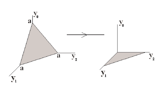
Figure 1: Figure 1a represents the Coxeter box of affine A₂ in the 3-space $\left(y_{0},y_{1},y_{2}\right)$. This is a triangle in 3-space with edges normal to the simple roots. Figure 1b gives its projection on the $\left(y_{1},y_{2}\right)$ plane which is also a triangle (a planar triangle).

The general group of quiver gauge symmetry in the UV regime involves obviously three factors as $U\left(N_{0}\right)\times U\left(N_{0}+N_{1}\right)\times U\left(N_{0}+N_{2}\right)$ with running gauge coupling constants $g_{0}$, $g_{1}$ and $g_{2}$ respectively. The factor $U\left(N_{0}\right)$ is engineered on the affine node of the Dynkin diagram of affine A₂ and $U\left(N_{0}+N_{1}\right)\times U\left(N_{0}+N_{2}\right)$ on the two other ordinary nodes. Along with these factors, there is also a diagonal $U_{D}\left(N_{0}\right)$ sub-symmetry that turns out to play a central role in the study of RG flows. It deals with the fundamental imaginary root $\delta$ of affine A₂ and has a zero vanishing beta function $\beta_{\delta}$. Its coupling constant is given by the type IIB string coupling constant $g_{s}$. In [13], RG cascades towards infrared has been shown to be accompanied by a decreasing of the charge of D3-branes ( $\Delta N_{0}<0$). This property has an interpretation not only in terms of Weyl reflections (Seiberg like duality) but also as translations in the root lattice generating the affine RG cascades. The decreasing of D3 charge is easily seen on the Cachazo et al picture using a formal analogy between flows in supersymmetric quiver gauge theories and dynamics of a classical particle with coordinates $X=\sum_{j=0}^{r}y_{j}\lambda_{j}$, $\alpha_{i}.\lambda_{j}=\delta_{ij}$, here $\lambda_{j}$s are the fundamental weights of the affine Lie algebra (affine A₂). Up to translations, the dynamics of the $X$ particle is restricted inside the affine A₂ Coxeter box defined by,

$$g_{i}^{-2}\left(X\right)=\alpha_{i}\cdot X=y_{i}\geq 0,$$ (4.19)

where $\alpha_{i}$s are the usual simple roots of affine A₂. Note that this 3-dimensional particle is attached to the walls of the Coxeter box by $N_{0}+N_{1}+N_{2}$ strings. The particle is attached on each i-th Coxeter wall by $N_{i}$ strings of equal tension and their length is obviously given by $g_{i}^{-2}\left(X\right)=y_{i}$. Note also that for the case where the X particle is on the i-th wall, we have $g_{i}^{-2}\left(X\right)=0$. So divisors $y_{i}=0$ are in one to one correspondence with the simple roots $\alpha_{i}$ of the affine $A_{2}$ algebra. In this case, the $X$ vector is normal to $\alpha_{i}$. Figure 1a gives the Coxeter box for affine $A_{2}$ model in the plane $\left(y_{1},y_{2}\right)$.

Figure 2: It represents hyperbolic A₂ Coxeter box. We have four variables related as $g_{-}^{-1}=y_{0}+y_{1}+y_{2}$ and $g_{+}^{-1}=y_{-1}+g_{-}^{-1}$, ($a=g_{-}^{-1},$ $b=g_{+}^{-1}$). Note that $b-a$ is proportional to axion $\chi$. In the limit $\chi\rightarrow 0,$ this figure coincides with figure 1b..

Now using Cachazo et al mechanical analogy, RG flows in affine quiver gauge model have a nice representation as,

$$\frac{dX}{dt}=F,$$ (4.20)

where the force $F$ acting on the particle is given by $F=\sum_{j=0}^{2}\alpha_{j}N_{j}$. This equation of evolution is immediately obtained by using the explicit expression of the running gauge couplings ${g_{i}^{-2}}\left(\mu\right)=\frac{\beta_{i}}{8\pi^{2}}\ln\frac{\mu}{\Lambda_{i}}$ and setting $8\pi^{2}y_{i}\left(t\right)=\beta_{i}\left(t_{i}-t\right)$ with $t=-\ln\mu$ ( $dt=-d\mu/\mu>0$ for flows towards IR). In this picture Seiberg like duality is nicely described in terms of Weyl reflections on walls of the Coxeter box. They map $y_{i}$ variables to

$$y_{i}^{\prime}=y_{i}-K_{ij}y_{j},$$ (4.21)

where $K_{ij}$ is the affine $A_{2}$ Cartan matrix. Geometrically, this is interpreted as flop transition where a dual $S^{2}$ is blown up. An analogous description is valid for RG cascades except now they are associated with Weyl translations. However, in this case, the particle is diffused outside the fundamental domain of the Coxeter box. Nevertheless Weyl translations act as shift operators and allow to bring the particle back inside the fundamental domain. In hyperbolic A₂ model, the method is quite similar although the theory is non conformal. The gauge group is $U\left(N_{-1}\right)\times U\left(M_{0}\right)\times U\left(M_{0}+N_{1}\right)\times U\left(M_{0}+N_{2}\right)$, where we have set $M_{0}=N_{-1}+N_{0}$, and the corresponding gauge couplings are $g_{-1\text{,}}$ $g_{0}$, $g_{1}$ and $g_{2}$ respectively. This hyperbolic model has two diagonal sub-symmetries $U_{D}\left(N_{-1}\right)$ and $U_{D}\left(M_{0}\right)$ in one to one with the two fundamental imaginary roots $\delta$ and $\gamma$ and the $g_{-}$ and $g_{+}$ couplings eq(3.9). In the UV regime of $\mathcal{N}=2$ hyperbolic A₂, viewed as a deformation of affine A₂ UV theory, one is interested in positive definite beta functions ensured by requiring,

$$\beta_{1}=2N_{1}-N_{2}>0;\qquad\beta_{2}=2N_{2}-N_{1}>0.$$ (4.22)

These relations fix the range of allowed UV values of part of the gauge group ranks namely $U\left(M_{0}+N_{1}\right)\times U\left(M_{0}+N_{2}\right)$. For the other ranks $N_{0}$ and $N_{-1}$, the situation is a little bit subtle, the $U_{D}\left(N_{-1}\right)$ and $U_{D}\left(M_{0}\right)$ gauge factors are no longer conformal. The corresponding beta functions $\beta_{\gamma}$ and $\beta_{\delta}$ are negative because $\beta_{\gamma}=-N_{0}$ and $\beta_{\delta}=-N_{-1}$. But this is not a problem since what interest us in the study of RG flows is not the diagonal group but rather the gauge factors $U\left(N_{0}\right)$ and $U\left(N_{-1}\right)$ associated with the affine and hyperbolic nodes respectively. Like in affine case and because of stringy origin, their beta functions $\beta_{0}$ ( $\beta_{0}=-\left(N_{-1}+N_{1}+N_{2}\right)$) and $\beta_{-1}$ ( $\beta_{-1}=N_{-1}-N_{0}$) are not required to be positive. Therefore, we have to distinguish between different cases according to signs of these beta functions. Moreover, since $\beta_{0}$ is negative exactly like in affine case, it is then natural to adopt the same condition one uses in the affine model namely $N_{0}$ large enough with respect to the ranks $N_{1}$ and $N_{2}$; i.e,

$$2N_{0}>>N_{1}+N_{2}.$$ (4.23)

For the rank $N_{-1}$, it is fixed by the sign of $\beta_{-1}$. For $\beta_{-1}$ positive ( negative) definite, we should have $N_{-1}>N_{0}$ ($N_{-1}<N_{0}$) and for $\beta_{-1}=0$ we have $N_{-1}=N_{0}$. So in the UV regime of hyperbolic theory with positive $\beta_{-1}$, we should have the following conditions,

$$N_{-1}>N_{0}>N_{1};\qquad N_{-1}>N_{0}>N_{2}.$$ (4.24)

In this case, we dispose at least of two beta functions with opposite signs.

Cascades in hyperbolic theory:  To study RG cascades in hyperbolic A₂ quiver gauge model, we have to compute the variations of $N_{0}$ and $N_{-1}$ during cascading towards infrared and prove that the variation of the total charge of D3-branes $M_{0}=N_{0}+N_{-1}$ is negative. This condition, which extends what we know about cascades in affine quiver gauge theories, follows also from the fact that in hyperbolic gauge models the role of $\Delta N_{0}$ of affine models is played by $\Delta M_{0}$ as can be seen on the structure of the quiver gauge group. These two quantities should be related with the structure of the Weyl group in hyperbolic theory. Remember that like in affine case, the Weyl group W_hyp of hyperbolic algebras is also a semi-direct product between reflections W_finite and translations T. The main difference between W_hyp and W_aff groups is that in the former the set of translations is larger. This property follows from the fact that in hyperbolic symmetries one has two basic imaginary roots $\delta$ and $\gamma$ and so two fundamental translations T${}_{\alpha}^{\delta}$ and T${}_{\alpha}^{\gamma}$. These translations are indeed the generators of RG cascades in hyperbolic gauge models.

To get the variations of $N_{0}$ and $N_{-1}$, we borrow results from geometric unification of dualities in ordinary and affine supersymmetric quiver gauge theories and prove the following statements.

$$\Delta M_{0}<0;\qquad\text{\ but \ }\Delta N_{0}\text{ \ and \ }\Delta N_{-1}\text{ \ have indefinite sign}$$ (4.25)

To do so we start by recalling the way we get the negative sign of $\Delta N_{0}$ in $\mathcal{N}=1$ affine quiver gauge models. There, one uses a geometric approach which expresses $\Delta N_{0}$ as the product of the fluxes of $H_{NS}$ and $H_{RR}$ field strengths of F1 and D1 strings [13, 29],

$$\Delta N_{0}=8\pi^{2}\int_{B_{\delta}}H_{NS}\wedge\int_{A_{\delta}}H_{RR},$$ (4.26)

where the NS-NS and RR fields strengths can be usually decomposed as $H=\Sigma_{j}\alpha_{j}H^{\left(j\right)}$ and where A_δ and B_δ are three cycles to be described in a moment. This method of doing has an interpretation in terms of geometric transition in the underlying Calabi-Yau threefold Y₀ on which type IIB string is compactified. The point is that while Weyl reflections on walls of the Coxeter box are associated with Seiberg like duality, Weyl translations require crossing Coxeter box walls. This may be naively interpreted as associated with a geometric transition as suggested by geometric unification of dualities. This means that after transition, the initial variety Y₀ with an elliptic A₂ geometry get replaced by a new one denoted Y${}_{0}^{\prime}$ with dual pairs of three cycles. In field theory language, this geometric transition corresponds to switching on the non linear adjoint matter self-interactions $W\left(\Phi_{i}\right)=\sum_{l=1}^{k+1}\xi_{l}\Phi^{l}$, so $\mathcal{N}=2$ supersymmetry is partially broken and the affine quiver gauge theory has $\mathcal{N}=1$ supersymmetry. Because of non linearity of $W\left(\Phi_{i}\right)$, the Calabi-Yau threefold Y₀ undergo a geometric transition where the two cycles S${}_{i}^{2}$ of the deformed elliptic singularity get replaced by three cycles involving S${}_{i}^{3}$s. Moreover D5-branes get replaced by their fluxes. The resulting generalized conical geometry Y${}_{0}^{\prime}$ contains then a particular pair of dual three cycles A_δ and B_δ, the sub-index $\delta$ recalls that they have been generated out of the closed two cycle C_δ of Y₀. By integration of the relations,

$$\int_{B_{\delta}}H_{NS}^{\left(i\right)}=\Delta\left(g_{i}^{-2}\right)=R_{i};\qquad\int_{A_{\delta}}H_{R}^{\left(i\right)}=N_{i},$$ (4.27)

and using the fact that $\Delta\left(g_{i}^{-2}\right)=-\beta_{i}\ln\frac{\mu_{1}}{\mu_{2}}$ ($\mu_{1}>\mu_{2}$) which in mechanical analogy can be also put in the form $R_{i}=-aN_{i}$ [13], we get $\Delta N_{0}=-aN^{2}$ which is negative definite as far as there are D5-brane charges. Negativity of $\Delta N_{0}$ follows of course from the fact that eigenvalues of ordinary A₂ Cartan matrix are positive definite. In the $\mathcal{N}=1$ hyperbolic quiver gauge model, the situation is quite similar to the above affine discussion. By switching on the non linear potential $W$, the initial Calabi-Yau threefold Y_- with hyperbolic geometry ( extending previous Y₀ having an elliptic geometry) undergoes a geometric transition leading to Y${}_{-}^{\prime}$. The two cycles S${}_{i}^{2}$ of initial Y_- get replaced by three cycles S${}_{i}^{3}$. The resulting generalized conical geometry Y${}_{-}^{\prime}$ contain then two pairs of dual closed three cycles $\left(A_{\delta},B_{\delta}\right)$ and $\left(A_{\gamma},B_{\gamma}\right)$. Extending the previous affine analysis, we can write down immediately the variations $\Delta M_{0}$ and $\Delta N_{-1}$ during cascading in hyperbolic theory. For the value of $\Delta M_{0}$, we have a similar relation as in eq(4.26),

$$\Delta M_{0}=8\pi^{2}\int_{B_{\delta}}H_{NS}\wedge\int_{A_{\delta}}H_{RR},$$ (4.28)

which, by help of previous results, reads as $\Delta M_{0}=-a\sum_{i,j=0}^{r}K_{ij}N_{i}N_{j}$, $a>0$. Because of the identity $\sum_{i,j=0}^{r}K_{ij}d_{i}d_{j}=0$, this is a negative quantity as far as $N_{i}$’s are non zero. This proves our first statement. For the second statement, it is enough to note that the variation $\Delta N_{-1}$ is linked with the imaginary root $\gamma$. So we have,

$$\Delta N_{-1}=8\pi^{2}\int_{B_{\gamma}}H_{NS}\wedge\int_{A_{\gamma}}H_{RR}.$$ (4.29)

The evaluation of this relation is similar to the computation of $\Delta M_{0}$ (4.28), except now we have more general sums as shown on the following explicit expression $\Delta N_{-1}=-aN^{2}=-a\sum_{i,j=-1}^{r}K_{ij}N_{i}N_{j}$. Since in hyperbolic Lie algebras, $N^{2}$ has an indefinite sign, we find that the sign of the variation of $N_{-1}$ during cascades towards infrared is indeed indefinite. Finally by help of the relation $M_{0}=N_{0}+N_{-1}$, we can compute the variation of $N_{0}$, we get $\Delta N_{0}=\Delta M_{0}-\Delta N_{-1}$ which has also an indefinite sign.

5 Conclusion and Comments

In this paper, we have studied the classification of four dimensional supersymmetric quiver gauge theories which can be embedded in type II strings on Calabi-Yau threefolds. We have shown that there are three basic classes in one to one with Vinberg classification theorem of Lie algebras. We have given their D-brane realizations and analyzed the corresponding RG flows towards infrared. Among our results, we quote the following:

(1) Along with supersymmetric ordinary and affine ADE quiver gauge models, there is an indefinite class associated with the indefinite sector of Lie algebras sharing most features of usual ordinary and affine supersymmetric quiver gauge models. Except few tentatives for extensions such the one on duality walls [27, 28], see also [30], this indefinite sector has not been explored before. This is mainly due to the lack of complete Lie algebraic results in this matter. However despite this difficulty, we have shown that one can make a quite precise idea about the structure of indefinite quiver gauge theories by looking at their interesting hyperbolic subset. The latter which may be thought of as simplest generalizations of affine models, can be used as a laboratory to establish characteristic results of indefinite gauge theories.

(2) As far as hyperbolic models are concerned, we have shown that these supersymmetric gauge theories have very special features. They can be viewed as low energy limit of type IIB string on CY3s with hyperbolic ADE geometry and are, surprisingly, strongly linked with the RR axion $\chi$. They have D-brane realizations depending on the sign of $\chi$ modulus interpreted as the volume of the cycle $S_{\chi}^{2}$ associated with the hyperbolic node. According to the signs of $\chi$, we have distinguished three kinds of models:
(i) Minimal hyperbolic model associated with $\chi<0$. The word minimal means that there is no D5-brane wrapping the hyperbolic two cycle.
(ii) Non minimal hyperbolic model with $\chi>0$ and partially wrapped D5-branes on $S_{\chi}^{2}$.
(iii) Finally models with $\chi=0$ coinciding exactly with the usual affine quiver gauge theory.

(3) We have studied RG cascades in hyperbolic quiver gauge theories. We have shown that they are also linked with Weyl translations generating a part of automorphisms of the root system of hyperbolic Lie algebras as in case of affine gauge models. We have found that during cascading towards infrared the variations of the D3-brane charges $\Delta N_{0}$ and $\Delta N_{-1}$ have indefinite signs but their sum $\Delta N_{0}+\Delta N_{-1}$ giving the total D3-brane charge is negative. This result has been derived by help of the mechanical analogy of [13], but might be done as well by using the Klebanov-Strassler and Fiol procedures.

On the other hand and as far as supersymmertic field theory is concerned, we believe that the field theoretical results we have got for hyperbolic model such as computation of beta functions and cascades are valid as well for supersymmetric indefinite quiver gauge theories. Moreover and despite that these are non conformal, we have shown that hyperbolic, and more generally indefinite, quiver gauge theories share features we have in ordinary and affine cases. For instance, starting from a $\mathcal{N}=2$ hyperbolic (indefinite) gauge model, we can build $\mathcal{N}=1$ ones from geometric transition scenario. In field theoretical approach, it is enough to switch on the non linear adjoint matter self-interactions $W\left(\Phi_{i}\right)=\sum_{l=1}^{k+1}\xi_{l}\Phi^{l}$ with mass scales $W_{i}^{\prime\prime}=\Delta$ and proceed following [11, 13]. One can also study RG flows à la Klebanov-Strassler by computing the $\mathcal{N}=1$ physical beta functions $\beta_{i}^{phys}$. For running energies $\mu$ larger than scales $\Delta$, the superpotentials may be neglected and the $\mathcal{N}=1$ one loop holomorphic beta functions remain quite same as in $\mathcal{N}=2$ case,

$$\beta_{i}^{N=1}\sim\beta_{i}^{N=2};\qquad\Lambda_{i}^{\mathcal{N}=1}\sim\Lambda_{i}\qquad\mu>>\Delta.$$ (5.1)

Below $\Delta$, adjoint matter acquires mass and the $\mathcal{N}=1$ holomorphic beta functions $\beta_{i}^{low}$ as well as the corresponding gauge scales $\Lambda_{i}^{low}$ get modified as,

$$\beta_{i}^{low}=N_{i}+\beta_{i};\qquad\ln\left(\Lambda_{i}^{low}\right)=\frac{\beta_{i}}{\beta_{i}^{low}}\ln\left(\Lambda_{i}\right)+\frac{N_{i}}{\beta_{i}^{low}}\ln\left(\Delta\right).$$ (5.2)

To get the RG flows in $\mathcal{N}=1$ hyperbolic ( indefinite) quiver gauge theories described by the action (2.3), one rather needs the NSVZ physical beta functions for gauge and matters[31]. These are obtained by extending affine analysis of [13] to the hyperbolic (indefinite) case.

Above $\Delta$, we get

$$\beta_{i}^{phys}=\sum_{j}K_{ij}^{-}N_{j}+\mathrm{\gamma}_{i}N_{i}+\sum_{j\neq i}\mathrm{\eta}_{ij}\left|K_{ij}^{-}\right|N_{j};\qquad\beta_{ij}^{phys}=\beta_{ij}=\mathrm{\gamma}_{i}+2\mathrm{\eta}_{ij},$$ (5.3)

where $\mathrm{\gamma}_{i}=\mathrm{\gamma}\left(\Phi_{i}\right)$ and $\mathrm{\eta}_{ij}=\mathrm{\eta}\left(Q_{ij}\right)$ are respectively the anomalous dimensions of massive adjoint and bi-fundamental matters and where we have set $\beta_{i}^{phys}=\beta\left(g_{i}^{phys}\right)$ and $\beta_{ij}^{phys}=\beta\left(\lambda_{ij}^{phys}\right)$. The above eq can be also rewritten into a combined form as $\beta_{i}^{phys}=\frac{\mathrm{\gamma}_{i}+2}{2}\left[2N_{i}-\sum_{j\neq i}\frac{\left(\beta_{ij}-\mathrm{\gamma}_{i}-2\right)}{\mathrm{\gamma}_{i}+2}K_{ij}^{-}N_{j}\right]$.

Below $\Delta$, the $\mathrm{\gamma}_{i}$ anomalous dimensions can be set to one, so the above beta functions reduces to $\beta_{i}=\frac{3}{2}\left(2N_{i}+\sum_{j\neq i}\frac{\left(\beta_{ij}-\mathrm{3}\right)}{\mathrm{3}}\left|K_{ij}\right|N_{j}\right)$. For marginal quartic superpotential $Tr\left[\left(Q_{ij}Q_{ij}\right)^{2}\right]$ and if moreover $\beta_{ij}=0$, the anomalous dimensions $\mathrm{\eta}_{ij}$ become minus half and so the above $\mathcal{N}=1$ beta functions reduce to $\beta_{i}=\frac{\mathrm{\gamma}_{i}+2}{2}K_{ij}N_{j}$ which should be compared with the value of $\mathcal{N}=2$ hyperbolic (indefinite) quiver gauge model.

In the end of this discussion, we would like to make a note concerning embedding of indefinite quiver gauge theories in type IIB string compactification on CY threefolds. While hyperbolic quiver gauge models have a meaningful type IIB string interpretation, indefinite generalizations need however more explorations. For instance in the former subset, the gauge coupling associated with the hyperbolic node is strongly linked with the RR axion field, but for indefinite case the situation deserves more analysis.

Acknowledgement 1

This research work on brane physics enters in the framework of Protars III/D12-25/CNR (2003) Rabat. E.H Saidi would like to thank CNR/CSIC for support and Cesar Gomez for kind hospitality at ITF Madrid where part of this work has been done. The work of A.Belhaj is supported by Ministerio de Educación Cultura y Deportes, (Spain) grant SB 2002-0036. R.Ahl Laamara and L.B.Drissi are so grateful to high Energy section of ICTP for kind hospitality.

6 Appendices

Here we give two appendices, one regarding root system of indefinite Lie algebras and the other deals with hyperbolic ADE quiver gauge theories.

6.1 Appendix A: Indefinite Lie algebras

Like for ordinary and affine Kac-Moody ADE Lie algebras, a nice way to approach indefinite simply laced Lie algebras is in terms of simple roots $\alpha{{}_{i};}$ ${i=1,...,n}$ and corresponding Cartan matrices $K_{ij}$. From axiomatic point of view, these require the knowledge of the triplet $(\mathbf{\hbar},\Pi,\Pi^{\nu})$ defining respectively commuting Cartan generators ${H_{i}}$, the basis of simple roots ${\alpha}{{}_{i}}$ and the basis of their duals. In representation theory; and too particularly in quantum field theory, this triplet corresponds to specifying the commuting observables and the basic quantum excitation operators. With these simple roots, one may encode most of algebraic features of Lie algebras including indefinite ones. For instance, whenever there exists a bi-linear form (,), the Cartan matrix of simply laced indefinite Lie algebras can be realized as usual as

$$K_{ii}=2;\qquad K_{ij}=2\frac{(\alpha_{i},\alpha_{j})}{(\alpha_{i},\alpha_{i})}\in\mathbb{Z}_{-}\text{ \ for\ \ }i\neq j,$$ (6.1)

which is equal to $K_{ij}=\alpha_{i}.\alpha_{j}$ seen that $\mathbf{(}\alpha_{i},\alpha_{i}\mathbf{)}=2$. For this class of indefinite symmetrizable simply laced Lie algebras, the statement that $K_{ij}$ is the Cartan matrix of an indefinite Lie algebra means that for some real positive definite vector $\mathbf{x}\in\mathbf{\hbar}$, we have,

$$K_{ij}x_{j}=-y_{i}<0;\qquad i,j=1,2,...,n,$$ (6.2)

where $x_{j}>0$, $j=1,2,...,n$ are components of $\mathbf{x}$ and $y_{i}$ are also positive, hence $\left(-y_{i}\right)$ are negative definite. The negative sign in front of $(-y_{i})$ is remarkable since it has an interesting geometric interpretation indicating that the space $\mathbf{\hbar}$ has an indefinite signature with a pseudo-euclidean metric. This metric extends the Lorentzian signature of usual affine symmetries. Because of this indefinite signature, indefinite Lie algebras are still a mathematical open subject. For instance their classification has not yet been achieved. Nevertheless, there are some subsets of these indefinite symmetries where there are exact results. One of these subsets the hyperbolic sub-class considered in this paper. According to W. Li classification, there are $238$ hyperbolic Lie algebras containing the following special simply laced list,

$$\mathcal{H}_{1}^{4},\quad\mathcal{H}_{2}^{4},\quad\mathcal{H}_{3}^{4},\quad\mathcal{H}_{1}^{5},\quad\mathcal{H}_{8}^{5},\quad\mathcal{H}_{1}^{6},\quad\mathcal{H}_{5}^{6},\quad\mathcal{H}_{6}^{6},\quad\mathcal{H}_{1}^{7},$$

$$\mathcal{H}_{1}^{7},\quad\mathcal{H}_{1}^{8},\quad\mathcal{H}_{4}^{8},\quad\mathcal{H}_{5}^{8},\quad\mathcal{H}_{1}^{9},\quad\mathcal{H}_{4}^{9},\quad\mathcal{H}_{5}^{9},\quad\mathcal{H}_{1}^{10},\quad\mathcal{H}_{4}^{10}.$$ (6.3)

For instance, $\mathcal{H}_{3}^{4}$ is just the hyperbolic extension of affine A${}_{2}^{\left(1\right)}$. More details on this sub-classification as well as applications of hyperbolic invariance may be found in [24],[25],[14, 15] and refs therein.

6.2 Appendix B: Hyperbolic ADE models

Depending on the values of quiver gauge group ranks given by the charge of regular D3 and fractional D5-branes, beta function components in hyperbolic ADE models can have arbitrary signs. In general, each $\beta_{i}$ factor can be either positive ( $\beta_{i}>0$), zero ( $\beta_{i}=0$) or negative ( $\beta_{i}<0$). This last property shows that the study of the RG flows in hyperbolic gauge models depends on these signs. To have an idea on how to get and fix these signs, we start from the general formula of holomorphic beta functions in $\mathcal{N}=2$ hyperbolic gauge models,

$$\beta_{i} = \sum_{j=-1}^{r}K_{ij}\widehat{N}_{j};\qquad-1\leq i\leq r,$$

$$\beta_{\delta} = \sum_{i=0}^{r}d_{i}\beta_{i}=d_{0}\beta_{0}+\beta_{\psi},$$ (6.4)

$$\beta_{\gamma} = \sum_{i=-1}^{r}d_{i}\beta_{i}=d_{-1}\beta_{-1}+\beta_{\delta},$$

then solve them by using Lie algebra results. First note that because of the identity $\sum_{j=0}^{r}K_{ij}d_{j}=0$ and using the fact that $K_{-1j}=0$ for $1\leq j\leq r$, the first relation of above eqs has a kernel which leads to a remarkable simplification. Indeed taking the ranks as $\widehat{N}_{i}=Md_{i}$, we have

$$b_{i}=\sum_{j=-1}^{r}K_{ij}\widehat{N}_{j}=M\left(K_{-1i}d_{-1}+\sum_{j=0}^{r}K_{ij}d_{j}\right)=MK_{-1i}d_{-1}$$ (6.5)

which is non zero only for $b_{-1}=2Md_{-1}$ and $b_{0}=-Md_{-1}$. As a consequence of this feature, the beta functions $\beta_{i}$, $1\leq i\leq r$ of hyperbolic ADE quiver gauge theories are independent on the number of regular branes; they behave exactly as in ordinary ADE quiver gauge models. So, the quantity $\sum_{j=-1}^{r}K_{ij}\widehat{N}_{j}$ reduces to

$$\beta_{-1} = N_{-1}-N_{0};\qquad\beta_{0}=-\left(N_{-1}+\sum_{j=1}^{r}\left|K_{0j}\right|N_{j}\right)<0,$$ (6.6)

$$\beta_{i} = \sum_{j=1}^{r}K_{ij}N_{j};\qquad 1\leq i\leq r,$$

showing that the previous results gotten for hyperbolic A_r models are also valid for hyperbolic DE ones. Therefore in hyperbolic ADE gauge theories, $\beta_{0}$ is usually negative and the sign of $\beta_{-1}$ is given by the signature of $\left(N_{-1}-N_{0}\right)$. To get the sign of remaining $\beta_{i}$; we consider the UV regime where $\mu>\Lambda_{i}$ with $1\leq i\leq r$. This domain can be represented in a simpler way by ordering gauge scales $\Lambda_{i}$ as $\Lambda_{1}>\Lambda_{2}>...>\Lambda_{r}$. In this parameterizations, positivity condition of beta components translates into $\mu>\Lambda_{1}$. This domain has a nice interpretation in Lie algebra language. Precisely it corresponds to the Vinberg phase which states that there usually exists a configuration

$$\mathbf{N}=\left(N_{1}^{\left(0\right)},...,N_{r}^{\left(0\right)}\right);\qquad N_{i}>0,$$ (6.7)

such that $\beta_{i}>0$ with $1\leq i\leq r$. So UV regime in ordinary supersymmetric quiver gauge theories corresponds to Vinberg configuration in finite dimensional Lie algebras. As Vinberg theorem is in connection with RG flows in supersymmetric quiver gauge theories, we will give details on this issue. The system (6.4) defining $\beta_{i}$s is very impressive; it recalls the Vinberg theorem on Lie algebras classification. This theorem states that for any Lie algebra, there exists two positive real vector $\mathbf{u}=\left(u_{1},...,u_{n}\right)$ and $\mathbf{v}=\left(v_{1},...,v_{n}\right)$ such that,

$$\sum_{\rho}K_{\mu\rho}^{\left(q\right)}u_{\rho}=qv_{\rho}$$ (6.8)

where $K_{\mu\rho}^{\left(q\right)}$ with $q=+1,0,-1$ stand respectively for the Cartan matrices of ordinary, affine and hyperbolic ( indefinite) Lie algebras. In our case, the correspondence is given by $\mathbf{u\longleftrightarrow N}=\left(N_{-1},...,N_{r}\right)$ and $\mathbf{v\longleftrightarrow\beta}=\left(\beta_{-1},...,\beta_{r}\right)$. Following this theorem and using known results on geometric engineering on $\mathcal{N}=2$ supersymmetric QFT₄s [2, 14] stating that holomorphic beta functions are proportional to Lie algebra Cartan matrices, one sees that in general supersymmetric quiver gauge theories have three remarkable phases parameterized by the quantum number $q=-1,0,-1$. This quantum number captures the global signs of the beta function vector $\mathbf{\beta}=\left(\beta_{-1},...,\beta_{r}\right)$ and so we have the following correspondence:

$$q = +1\qquad\Longleftrightarrow\qquad\text{UV free }\mathcal{N}=2\text{ QFT}_{4}$$

$$q = 0\qquad\ \ \Longleftrightarrow\qquad\text{Conformal }\mathcal{N}=2\text{ QFT}_{4}$$ (6.9)

$$q = -1\qquad\Longleftrightarrow\qquad\text{Confined }\mathcal{N}=2\text{ QFT}_{4}.$$

According to $\beta_{i}$ signs (i.e $\beta_{i}>0$, $\beta_{i}=0$, $\beta_{i}<0$ ), there are $3^{n}$ others more.

References

- [1] A. Hanany, E. Witten, Type IIB Superstrings, BPS Monopoles, And Three-Dimensional Gauge Dynamics, Nucl.Phys. B492 (1997) 152-190, hep-th/9611230
-
[2]
S. Katz, A. Klemm and C. Vafa, Geometric Engineering of Quantum
Field Theories, Nucl.Phys. B497 (1997) 173-195, hep-th/9609239,
S. Katz, P. Mayr, C. Vafa, Mirror symmetry and Exact Solution of 4D N=2 Gauge Theories I, Adv.Theor.Math.Phys. 1 (1998) 53-114, hep-th/9706110 -
[3]
A. Belhaj, A. Elfallah and E.H. Saidi, On the affine D4 mirror
geometry, Class. Quantum Grav. 16 (1999) 3297-3306.
A. Belhaj, A. Elfallah and E.H. Saidi, On the non-simply laced mirror geometries in type II strings, Class. Quantum Grav. 17 (2000) 515-532. A. Belhaj, E.H. Saidi, Toric Geometry, Enhanced non Simply laced Gauge Symmetries in Superstrings and F-theory Compactifications, hep-th/0012131 - [4] A. Belhaj, L.B. Drissi, J. Rasmussen, On N=1 gauge models from geometric engineering in M-theory, Class.Quant.Grav. 20 (2003) 4973-4982, hep-th/0304019.
- [5] M. Ait Ben Haddou, E.H. Saidi, Explicit Analysis of Kahler Deformations in 4D N=1 Supersymmetric Quiver Theories, Physics Letters B575 (2003)100-110, hep-th/0307103.
- [6] R. Dijkgraaf, C. Vafa, Matrix Models, Topological Strings, and Supersymmetric Gauge Theories, Nucl.Phys. B644 (2002) 3-20, hep-th/0206255.
- [7] R. Dijkgraaf, C. Vafa, A Perturbative Window into Non-Perturbative Physics, hep-th/0208048.
- [8] R. Gopakumar, C. Vafa, On the Gauge Theory/Geometry Correspondence Adv.Theor.Math.Phys. 3 (1999) 1415-1443, hep-th/9811131
- [9] C. Vafa, Superstrings and Topological Strings at Large N, J.Math.Phys. 42 (2001) 2798-2817, hep-th/0008142
- [10] F. Cachazo, K. Intriligator, C. Vafa, A Large N Duality via a Geometric Transition, Nucl.Phys. B603 (2001) 3-41, hep-th/0103067.
- [11] F. Cachazo, S. Katz, C. Vafa, Geometric Transitions and N=1 Quiver Theories, hep-th/0108120.
-
[12]
F. Cachazo, C. Vafa, N=1 and N=2 Geometry from Fluxes,
hep-th/0206017.
R. Ahl Laamara, Memoire de DESA-PHE, Lab/UFR-HEP, Faculté des Sciences de Rabat (2003). - [13] F. Cachazo, B. Fiol, K. Intriligator, S. Katz, C. Vafa, A Geometric Unification of Dualities, Nucl.Phys. B628 (2002) 3-78, hep-th/0110028.
- [14] M. Ait Ben Haddou, A. Belhaj, E.H. Saidi, Geometric Engineering of N=2 CFT4s based on Indefinite Singularities: Hyperbolic Case, Nucl.Phys. B674 (2003) 593-614, hep-th/0307244
- [15] M. Ait Ben Haddou, A. Belhaj, E.H. Saidi, Classification of N=2 supersymmetric CFT4s: Indefinite Series, hep-th/0308005.
- [16] E.H Saidi (Ed), Contributions to Eigth workshop on QFT, Geometry and non perturbative physics, Proceedings on High Energy Physics, Lab/UFR-HEP, Rabat, (2003).
- [17] I.R. Klebanov, M. J. Strassler, Supergravity and a Confining Gauge Theory: Duality Cascades and SB-Resolution of Naked Singularities, JHEP 0008 (2000) 052, hep-th/0007191.
- [18] I.R. Klebanov, supergravity dual of cascading confining gauge theory, lecture notes at spring school on superstring theory and related topics, ICTP 2004.
- [19] D. Berenstein, On the universality class of the conifold, JHEP 0111 (2001) 060, hep-th/0110184,
- [20] M. Ait Ben Haddou, E.H. Saidi, Hyperbolic ADE Invariance: Root system and Weyl symmetries, Lab/UFR-HEP 0401/GNPHE 0401 (2004)
- [21] M. Ait Ben Haddou, These de doctorat, Algèbres de Lie affine, Formes hermitiennes et leurs Representations, Département de Mathématique, Faculté des Sciences de Rabat (1994).
- [22] J. Humphreys, Introduction to Lie algebras and Representation Theory, Springer Verlag (1972)
- [23] P. Goddard, D. Olive, Introduction to affine Kac-Moody algebras, Int Jour Mod Phys V1 (1996) 1.
- [24] W. Li, Classification of generalized Cartan Matrices of hyperbolic type, Chinese Annals of Math 9B (1988)68
- [25] V.G Kac, Infinite dimensional Lie algebras, Cambridge University Press (1990)
- [26] C. Vafa, Evidence for F-Theory, Nucl.Phys. B469 (1996) 403-418, hep-th/9602022.
- [27] B. Fiol, Duality cascades and duality walls, JHEP 0207 (2002) 058, hep-th/0205155.
- [28] A. Hanany, J. Walcher, On Duality Walls in String Theory, JHEP 0306 (2003) 055, hep-th/0301231
- [29] B. Giddings, S. Kachru, J. Polchinski, Hierarchies from Fluxes in String Compactifications, Phys.Rev. D66 (2002) 106006, hep-th/0105097.
-
[30]
A. Kleinschmidt, I. Schnakenburg, P. West, Very-extended
Kac-Moody algebras and their interpretation at low levels, Class.Quant.Grav.
21 (2004) 2493-2525, hep-th/0309198.
M. Henneaux, B. Julia, Hyperbolic billiards of pure D=4 supergravities, JHEP 0305 (2003) 047, JHEP 0305 (2003) 047 -
[31]
M. Shifman and A. Vainshtein, Nuc.Phys. B277 (1986) 456; Nuc.Phys. B539 (1991) 571,;
V.Novikov, M.Shifman, A. Vainshtein, and V.Zakharov, Nuc.Phys. B229 (1983) 381