The properties of Q-balls in the general case of a sixth order potential have been studied using analytic methods. In particular, for a given potential, the initial field value that leads to the soliton solution has been derived and the corresponding energy and charge have been explicitly evaluated. The proposed scheme is found to work reasonably well for all allowed values of the model parameters.

1 Introduction

A scalar field theory with a spontaneously broken $U(1)$ symmetry may contain stable nontopological solitons, the so-called Q-balls [1]-[2]. Q-balls are coherent states of complex scalar fields that carry a global $U(1)$ charge and can be understood as bound states of scalar particles which appear as stable classical solutions carrying a rotating time dependent internal phase. They are characterized by a conserved nontopological charge $Q$ (Noether charge) that ensures existence and stability [3]-[4].

The concepts associated with these solutions are quite general and occur in a wide variety of physical contexts [5]. Q-balls are allowed in supersymmetric extensions of the standard model that allow flat directions in the scalar potential. Flat directions in the Minimal Supersymmetric Standard Model (MSSM) [6] have been shown to exist. The conserved charge is associated with the $U(1)$ symmetries of baryons and leptons, while, the relevant $U(1)$ fields correspond to either squark or slepton particles. Thus, Q-balls can be thought of as condensates of a large number of either squark or slepton particles which can affect baryogenesis via the Affleck-Dine mechanism [7] during the post-inflationary period of the early universe. The Q-ball stability is cosmologically important since if stable Q-balls are formed in the early universe they can contribute to its dark matter content. These can be huge balls with charges of order $10^{20}$; however, very small Q-balls can also be considered as dark matter constituents [8]. Decaying Q-balls can also be of crucial cosmological significance. If Q-balls decay after the electroweak phase transition, they can protect baryons from the erasure of baryon number due to sphaleron transitions. Furthermore, the Q-ball decay may contribute to dark matter production in the form of the lightest supersymmetric particle, explaining the baryon to dark matter ratio of the universe [9].

Consider the $U(1)$ Goldstone model Lagrangian describing a single complex scalar field $\phi$ in three spatial dimensions given by

$${\cal L}=\frac{1}{2}\partial_{\mu}\phi\,\partial^{\mu}\bar{\phi}-U(|\phi|).$$ (1)

$U(|\phi|)$ has a single minimum at $\phi=0$ which is equivalent of stating that there is a sector of scalar particles (mesons) carrying $U(1)$ charge with mass equal to $\sqrt{\frac{1}{2}U^{\prime\prime}(0)}$. The corresponding energy functional is given by

$$E=\int\left(\frac{1}{2}|\dot{\phi}|^{2}+\frac{1}{2}|\nabla\phi|^{2}+U(|\phi|)\right)d^{3}x$$ (2)

while the conserved Noether current (due to the global $U(1)$ symmetry) is

$$J_{\mu}=\frac{1}{2i}\left(\bar{\phi}\,\partial_{\mu}\phi-\phi\,\partial_{\mu}\bar{\phi}\right)$$ (3)

with charge given by

$$Q=\frac{1}{2i}\int\left(\bar{\phi}\,\partial_{t}\phi-\phi\,\partial_{t}\bar{\phi}\right)d^{3}x.$$ (4)

The stationary Q-ball solution can be obtained by assuming that

$$\phi=e^{i\omega t}f(r)$$ (5)

where $f(r)$ is a real radial profile function that satisfies the ordinary differential equation

$$\frac{d^{2}f}{dr^{2}}+\frac{2}{r}\frac{df}{dr}=-\omega^{2}f+U^{\prime}(f)$$ (6)

with boundary conditions $f(\infty)=0$ and $f^{\prime}(0)=0$. In each case, the effective potential is defined as $U_{eff}(f)=\omega^{2}f^{2}/2-U(f)$, while, the existence of Q-ball solutions leads to constraints on the potential $U(f)$ and the frequency $\omega$: (i) The effective mass of $f$ must be negative, so, by assuming that $U(0)=U^{\prime}(0)=0$ and $U^{\prime\prime}(0)=\omega_{+}^{2}>0$ one can deduce that $\omega<\omega_{+}$. (ii) The minimum of $U(f)/f^{2}$ must be attained at some positive value of $f$ (say $0<f_{0}<\infty$) and existence of the solution requires that $\omega>\omega_{-}$ where $\omega_{-}^{2}=2U(f_{0})/f_{0}^{2}$. Hence, Q-balls exist for all $\omega$ in the range $\omega_{-}<|\omega|<\omega_{+}$.

The charge (4) and energy (2) of a stationary Q-ball solution (5) take the simple form

$$Q = 4\pi\omega\int r^{2}f^{2}(r)\,dr\$$ (7)

$$E = \frac{1}{2}\omega^{2}Q^{2}\,+4\pi\int\left(\frac{f^{\prime}{}^{2}}{2}+U(f)\right)r^{2}\,dr.$$ (8)

Numerical and analytical methods have shown that when the internal frequency is close to the minimal value $\omega_{-}$ the profile function is almost constant, implying that the charge (7) is large (thin-wall approximation). On the other hand, when the internal frequency approaches the maximal value $\omega_{+}$ the profile function falls off very quickly (thick-wall approximation). In the thick-wall approximation the behavior of $Q$ depends on the particular form of the potential and the number of dimensions [11].

The choice of the potential is not unique since the only requirement is that the ratio $U(f)/f^{2}$ has a local minimum at some value of $f$ different from zero. There are several natural types to be considered, two of which are shown below:

$$\mbox{I}:\hskip 14.22636ptU(f) = \frac{m_{1}^{2}}{2}f^{2}-\lambda_{1}f^{4}+\mu_{1}f^{6},$$

$$\mbox{II}:\hskip 14.22636ptU(f) = m_{3}f^{2}\left(1-K\log(\lambda_{3}f^{2})\right)+\mu_{3}f^{2p}.$$ (9)

In each case, two of the parameters can be removed by rescaling, thus, the potentials of type I have one free parameter while potentials of type II have two for fixed $p$. The type I potential is the simplest allowed one which is a polynomial in $f^{2}$, while type II mimics the D-flat direction in MSSM. Here, $p\geq 6$ is some integer that ensures the growth of the potential for large $f$, but does not destroy the flatness property for intermediate values of $f$. None of these types are the kind which might be associated with a renormalizable quantum field theory, but, they are typical of effective theories incorporating radiative or finite temperature corrections to a bare potential. In this paper, we shall be dealing with type I potentials only, for which $\omega_{+}=m_{1}$ and $\omega_{-}=\sqrt{\frac{2m_{1}^{2}\mu_{1}-\lambda_{1}^{2}}{2\mu_{1}}}$ . Stable Q-balls exist for $\sqrt{\frac{2m_{1}^{2}\mu_{1}-\lambda^{2}}{2\mu_{1}}}<\omega<m_{1}$. The equation of motion (6) is

$$\frac{d^{2}f}{dr^{2}}+\frac{2}{r}\frac{df}{dr}=\alpha^{2}f-4\lambda_{1}\,f^{3}+6\mu_{1}\,f^{5}.$$ (10)

where we have defined $\alpha^{2}=m_{1}^{2}-\omega^{2}$.

Q-balls can be studied either analytically [1, 11, 14], or numerically [3]-[13]. In a recent work [15, 16], we employed analytic arguments in order to construct an approximate profile function of the symmetrized Woods-Saxon type, expected to be valid in the thin-wall limit. This approximate profile led to an explicit energy-charge relation which, to our surprise, was found to yield valid results for a region far exceeding the expected limits of the thin-wall approximation. The calculation was carried out for a specific form of type I potential i.e. $\lambda_{1}=2$, $\mu_{1}=1$ and $m=2$. In this paper, the aforementioned work is being extended to include the general case of type I potentials (where the parameters are taken to be arbitrary) in both regimes, thin-wall and thick-wall respectively. This way, the soliton energy and charge as well as the initial field value $f(0)$ can be accurately derived as functions of $\alpha$ for the whole allowed range of the model parameters.

2 Potential Energy

From a mechanical point of view, a Q-ball solution describes the motion of a particle moving with friction in the potential

$$U_{eff}(f)=-\frac{1}{2}\,\alpha^{2}\,f^{2}+\lambda_{1}f^{4}-\mu_{1}f^{6},\hskip 14.22636pt\hskip 14.22636pt\lambda_{1},\mu_{1}>0.$$ (11)

The corresponding equation of motion is given by (10). Upon rescaling $r\rightarrow r/\alpha$ and letting $f(r)=f(0)\psi(ar)$ for $\psi(0)=1$, equation (10) transforms to

$$\frac{d^{2}\psi}{dr^{2}}+\frac{2}{r}\frac{d\psi}{dr}=\psi-4\lambda\psi^{3}+6\mu\psi^{5}$$ (12)

where $\lambda=\frac{\lambda_{1}f(0)^{2}}{\alpha^{2}}$ and $\mu=\frac{\mu_{1}f(0)^{4}}{\alpha^{2}}$ and the effective potential (11) becomes

$$U(\psi)=-\frac{1}{2}\,\psi^{2}+\lambda\,\psi^{4}-\mu\,\psi^{6}.$$ (13)

After some algebra, it can be shown that equation (12) implies that

$$\int_{0}^{\infty}r^{n-1}\left(\frac{d\psi}{dr}\right)^{2}dr=\frac{2n}{4-n}\int_{0}^{\infty}r^{n-1}\left(-\frac{1}{2}\psi^{2}+\lambda\psi^{4}-\mu\psi^{6}\right)dr,\hskip 14.22636ptn\neq 0.$$ (14)

For the special cases $n=3$ and $n=0$, we get that

$$\frac{1}{2}\int_{0}^{\infty}r^{2}\left(\frac{d\psi}{dr}\right)^{2}dr = 3\int_{0}^{\infty}r^{2}\left(-\frac{1}{2}\psi^{2}+\lambda\psi^{4}-\mu\psi^{6}\right)dr$$ (15)

$$2\int_{0}^{\infty}r^{-1}\left(\frac{d\psi}{dr}\right)^{2}dr = -\frac{1}{2}\psi(0)^{2}+\lambda\psi(0)^{4}-\mu\psi(0)^{6}$$ (16)

$$\equiv U(1).$$

The first condition is Derrick’s (or virial) theorem which states that, for a three dimensional model, the kinetic energy equals three times the potential energy; the second condition describes the energy dissipation of the mechanical system.

The mechanical analogue imposes several constraints on $U(1)$. Consider a particle initially located at the point $\psi(0)=1$ which starts rolling down the potential wall to eventually stop at the point $\psi(\infty)=0$. (Here $r$ corresponds to the time variable). Then, the potential energy (13) at the origin $U(1)=-\frac{1}{2}+\lambda-\mu$ has to be consumed by the friction term $\frac{2}{r}\frac{d\psi}{dr}$, therefore $U(1)$ has to be bounded both from below and above: since for $U(1)$ large the particle will overshoot the top point while for $U(1)$ small it will not reach it.

The initial potential energy $U(1)$ has to be positive implying that

$$\mu\leq\lambda-\frac{1}{2}$$ (17)

and, also, $U^{\prime}(1)$ has to be positive (attractive “force”) leading to

$$\mu\leq\frac{1}{6}\left(4\lambda-1\right).$$ (18)

These conditions are satisfied for $\lambda>1$ when (18) holds while for $1/2<\lambda<1$ when (17) holds. Note that for $\lambda<1$ no Q-ball solutions can be found. Depending on the shape of the potential (i.e. the actual values of $\lambda$ and $\mu$) the following two distinct cases occur:

I. Thin-Wall Approximation: In this case, $\psi(0)$ lies near the maximum of the effective potential which is deep. Then $U^{\prime}(1)=-1+4\lambda-6\mu\approx 0$ has to be positive and close to zero (slow roll) while $U^{\prime\prime}(1)$ is negative (convex region) and of order unity. The Q-ball solutions lie approximately on the line

$$\mu=\frac{1}{6}\left(4\lambda-1\right)$$ (19)

and the initial potential energy depends linearly on $\lambda$:

$$U(1)=\frac{1}{3}\left(\lambda-1\right),\hskip 14.22636pt\hskip 14.22636pt\lambda>1.$$ (20)

II. Thick-Wall Approximation: Here, the potential is shallow and the maxima are high up while $U^{\prime}(1)$ is positive and large (concave region) and $\mu$ is small. The initial potential energy $U(1)$ increases with $\lambda$ and reaches its maximal value when $\mu\rightarrow 0$. This value can be determined numerically and is found to be: $\lambda_{max}\simeq 4.70137$. The actual functional dependence of $U(1)$ on $\lambda$ however, is unknown and needs to be determined.

To that end, let us assume a leading power law behaviour

$$U(1)=\kappa\lambda^{n}.$$ (21)

Then, (13) implies that the Q-ball solutions lie on the line

$$\mu=-\frac{1}{2}+\lambda-\kappa\lambda^{n}$$ (22)

which determines $\kappa$ in terms of $\lambda_{max}$ (since $\mu(\lambda_{max})=0$):

$$\kappa=\frac{2\lambda_{max}-1}{2\lambda_{max}^{n}}.$$ (23)

In order to determine the value of $n$ in (21), we require that the transition from the thick-wall region to the thin-wall one be smooth implying that, $U^{\prime}(1)$ is small for small values of $\lambda$ ($\simeq 1)$, i.e.

$$U^{\prime}(1)=2(1-\lambda)+6\kappa\lambda^{n}\approx 0.$$ (24)

Its minimum value occurs at the point $\lambda_{\min}=\left(3n\kappa\right)^{\frac{1}{{1-n}}}$. Substituting $\lambda_{\min}$ in (24) one gets that $U^{\prime}(1)$ vanishes for $n=2.82187$ in which case $\lambda_{\min}=1.54889$ (in agreement to our hypothesis). Assuming that $n$ can only take integer or half integer values (otherwise the structure of the model on the complex plane would be very complicated), Figure [1] shows that for $n=3$, the transition is indeed satisfactorily smooth. For this case, we get that $\kappa=\frac{1}{24.75}$ . This way, we get the $\mu(\lambda)$ relation for the thin-wall (19) and thick-wall (22) limits depicted in Figure [2] against numerical data.

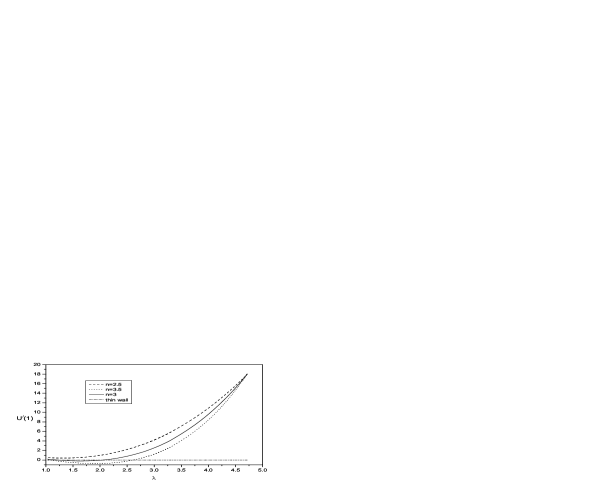
Figure 1: The potential energy gradient in terms of $\lambda$ for different values of $n$.

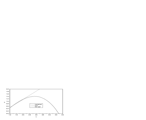
Figure 2: The $\mu(\lambda)$ relation for $n=3$ against numerical data.

3 Properties of Q-balls

Using the rescaling formulae of the previous section, the $\alpha$ dependence of the functions $E$, $Q$ and $f(0)$ can now be analytically determined. The initial field value $f(0)$ that leads to a Q-ball solution is given by

$$f(0)=\alpha\sqrt{\frac{\lambda}{\lambda_{1}}},\hskip 14.22636pt\alpha=\sqrt{\frac{\mu}{\mu_{1}}}\frac{\lambda_{1}}{\lambda}.\$$ (25)

Figure [3] depicts predicted values of $f(0)$ in terms of $\alpha$ against numerically calculated ones for sample values $\lambda_{1}=2$, $\mu_{1}=1$, $m=2$ (as in [16]).

Figure 3: Predicted initial field values $f(0)$ against numerical data.

The corresponding charge (7) and energy (8) functionals are given by:

$$Q = \frac{4\pi\omega}{\alpha}\frac{\lambda}{\lambda_{1}}\int_{0}^{\infty}\psi^{2}\,r^{2}dr$$ (26)

$$E = \frac{\alpha^{2}+2\omega^{2}}{2\omega}\,Q+4\pi\alpha\frac{\lambda}{\lambda_{1}}\int_{0}^{\infty}\left(\frac{1}{2}\,\psi^{\prime}{}^{2}-\lambda\,\psi^{4}+\mu\,\psi^{6}\right)r^{2}dr\ \cdot$$ (27)

It was shown in [16] that a trial function satisfying the boundary conditions and having the right asymptotic behavior, is the symmetrized Woods-Saxon profile

$$\phi(r)=\frac{c}{\sqrt{1+c_{1}\cosh\left(br\right)}}.$$ (28)

This function satisfies the exact differential equation

$$\phi^{\prime\prime}=\frac{b^{2}}{4}\phi-\frac{b^{2}}{c^{2}}\phi^{3}+\frac{3}{4}\frac{b^{2}}{c^{4}}\left(1-c_{1}^{2}\right)\phi^{5}$$ (29)

and the approximate one

$$\phi^{\prime\prime}+\frac{2}{r}\phi^{\prime}=\frac{b^{2}}{4}\left(1-\frac{4}{br}\right)\phi-\frac{b^{2}}{c^{2}}\left(1-\frac{1}{br}\right)\phi^{3}+\frac{3b^{2}}{4c^{4}}\left((1-c_{1}^{2})+\frac{2}{3}\frac{c_{1}^{2}}{br}~{}\right)\phi^{5}+O\left(\phi^{7}\right).$$ (30)

Here, $c$, $c_{1}$ and $b$ are arbitrary parameters which need to be determined in order that (28) fits the exact profile function $\psi(r)$ in the best possible way. Note that only two of the three parameters in (28) are independent since the initial condition $\phi(0)=1$ implies that $c=\sqrt{1+c_{1}}$.

First note that (28) satisfies the following relations:

$$\phi^{\prime}{}^{2} = \frac{b^{2}}{4}\,\phi^{2}-\frac{1}{2}\,\frac{b^{2}}{c^{2}}\,\phi^{4}+\frac{1}{4}\frac{b^{2}}{c^{4}}\left(1-c_{1}^{2}\right)\phi^{6}$$

$$\phi^{4} = c^{2}\phi^{2}+c^{2}c_{1}\frac{d}{dc_{1}}\phi^{2}$$

$$\phi^{6} = c^{4}\phi^{2}+2c^{4}c_{1}\frac{d}{dc_{1}}\phi^{2}+\frac{1}{2}c^{4}c_{1}^{2}\frac{d^{2}}{dc_{1}^{2}}\phi^{2}$$ (31)

in terms of which the charge (26) and energy (27) functionals can be explicitly evaluated:

$$Q = \frac{4\pi\omega}{\alpha}\frac{\lambda}{\lambda_{1}}\,\frac{c^{2}}{3b^{3}}\,i_{0}$$ (32)

$$E = 4\pi\frac{c^{2}}{3b^{3}}\sqrt{\frac{\mu}{\mu_{1}}}\bigg{\{}\left(\frac{\left(m^{2}+\omega^{2}\right)}{2\alpha}\frac{\lambda}{\lambda_{1}}\sqrt{\frac{\mu_{1}}{\mu}}+\mu c^{4}-\lambda c^{2}-\frac{1}{8}b^{2}c_{1}^{2}\right)i_{0}+\left(2\mu c^{4}-\lambda c^{2}-\frac{1}{4}b^{2}c_{1}^{2}\right)c_{1}\frac{di_{0}}{dc_{1}}$$ (33)

$$+\frac{1}{2}\left(\mu c^{4}+\frac{1}{8}b^{2}\left(1-c_{1}^{2}\right)\right)c_{1}^{2}\frac{d^{2}i_{0}}{dc_{1}^{2}}\bigg{\}}.$$

Here $i_{0}$ is a function of $c_{1}$ given by

$$i_{0}\left(c_{1}\right)=\frac{1}{\sqrt{1-c_{1}^{2}}}\,\mbox{arccosh}\left(\frac{1}{c_{1}}\right)\left[\pi^{2}+\mbox{arccosh}\left(\frac{1}{c_{1}}\right)^{2}\right],\hskip 14.22636pt\mbox{for}\hskip 14.22636ptc_{1}<1.$$ (34)

Note that $\lambda_{1}$, $\mu_{1}$, $m$ are fixed external parameters, $\lambda$ varies continuously between $1$ and $4.70137$ and $\mu$ is a known function of $\lambda$ given by (19) or (22) depending on the regime.

The profile parameters $b$ and $c_{1}$ can be determined by imposing the conditions (15) and (16) on $\phi(r)$, that is

$$\frac{1}{2}\,b^{2}c_{1}^{2}\,c^{2}\int_{0}^{\infty}\frac{dr}{r}\frac{\sinh^{2}r}{\left(1+c_{1}\cosh r\right)^{3}}=U(1)\hskip 14.22636pt\hskip 14.22636pt\hskip 14.22636pt\hskip 14.22636pt\hskip 14.22636pt\hskip 14.22636pt$$ (35)

$$\left(\frac{1}{2}-\lambda c^{2}+\mu c^{4}-\frac{b^{2}c_{1}^{2}}{24}\right)i_{0}+\left(2\mu c^{4}-\frac{b^{2}c_{1}^{2}}{12}-\lambda c^{2}\right)c_{1}\frac{di_{0}}{dc_{1}}+\frac{c_{1}^{2}}{2}\left(\mu c^{4}+\frac{b^{2}}{24}\left(1-c_{1}^{2}\right)\right)\frac{d^{2}i_{0}}{dc_{1}^{2}}=0.$$ (36)

Equations (35) can be written in a compact form

$$b=\,\frac{1}{c_{1}c}\,\sqrt{\frac{2U(1)}{i_{1}}}$$ (37)

where

$$i_{1}=\int_{0}^{\infty}\frac{dr}{r}\,\frac{\sinh^{2}r}{\left(1+c_{1}\,\cosh r\right)^{3}}$$ (38)

in terms of which (36) becomes

$$\left(\frac{1}{2}-\lambda c^{2}+\mu c^{4}-\frac{1}{12c^{2}}\,\frac{U(1)}{i_{1}}\right)i_{0}+\left(2\mu c^{4}-\frac{1}{6c^{2}}\,\frac{U(1)}{i_{1}}-\lambda c^{2}\right)c_{1}\frac{di_{0}}{dc_{1}}+\frac{c_{1}^{2}}{2}\left(\mu c^{4}+\frac{\left(1-c_{1}^{2}\right)}{12c_{1}^{2}c^{2}}\frac{U(1)}{i_{1}}\right)\frac{d^{2}i_{0}}{dc_{1}^{2}}=0.$$ (39)

Equation (39) determines $c_{1}$ in terms of $\lambda$ and and is depicted in Figure [4]. Note that the values of $c_{1}$ and $b$ obtained this way are universal since they do not depend on the geometrical parameters of the potential. Nevertheless, the values of the energy and charge do depend on the specific form of the potential i.e. the values of $\lambda_{1}$, $\mu_{1}$ and $m$. These values tend to infinity in both limits since (i) in the thin-wall limit $c_{1}\rightarrow 0$ while (ii) in the the thick-wall limit $b\rightarrow 0$.

Figure 4: The $c_{1}(\lambda)$ relation obtained from (39).

Figures [5] and [6] presents the $\alpha$ dependence of the charge (32) and energy (33) against values obtained numerically, for $\lambda_{1}=2$, $\mu_{1}=1$, $m=2$. It is interesting to realize that the range of validity of the thick-wall approximation is very wide and gives satisfactory results even in the thin-wall region. It appears that in this class of theories the Q-balls prefer to be “thick”.

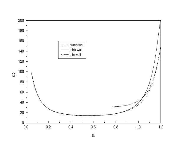
Figure 5: The $\alpha$ dependence of $Q$ given by (32).

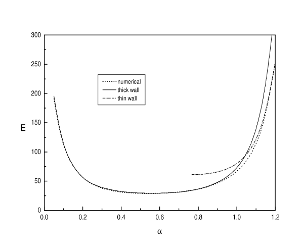
Figure 6: The $\alpha$ dependence of $E$ given by (33).

4 Conclusions

In this paper we have extended our earlier work [16] and investigated phenomenologically relevant properties of Q-balls in a universal way. In particular, we have addressed the following problem: Given the geometrical characteristics of the scalar potential find the initial field value that will lead to a Q-ball solution as well as the corresponding charge and energy of the soliton. For a particular class of potentials (sixth order polynomials), after parameter rescaling, the problem can be tackled in a universal way. The Q-ball profile can be accurately approximated by means of a two-parameter symmetrized Woods-Saxon function which can be analytically calculated in all cases. This scheme is found to yield satisfactory results in the whole parameter region so that we do not have to rely on approximations like thin-wall or thick-wall. The soliton energy and charge can subsequently be analytically calculated and compared against numerically calculated values taken from an earlier work [15].

We believe that a similar line of argument can be applied to study the profile function and the energy-charge dependence in all types of potentials.

References

- [1] S. Coleman, Nucl. Phys. B 262, 263 (1985)
- [2] T.D. Lee, Particles Physics and Introduction to Field Theory, Harwood, London (1981)
- [3] J.K. Drohm, L.P. Yok, Y.A. Simonov, J.A. Tyon and V.I. Veselov, Phys. Lett. B 101, 204 (1981)
- [4] T.I. Belova and A.E. Kudryavtsev, JETP 68, 7 (1989)
- [5] D.K. Hong, J. Low Temp. Phys. B 71, 483 (1998)
- [6] A. Kusenko, Phys. Lett. B 405, 108 (1997)
- [7] I. Affleck, M. Dine, Phys. Lett. B 249, 361 (1985)
- [8] A. Kusenko, M. Shaposhnikov, Phys. Lett. B 418, 46 (1998)
- [9] K. Enqvist, J. McDonald, Nucl. Phys. B 538, 321 (1999)
- [10] A. Kusenko, Phys. Lett. B 404, 285 (1997)
- [11] F. Paccetti Correia, M.G. Schmidt, Eur. Phys. J. C 21, (2001) 181
- [12] G. Rosen, J. Math. Phys. 9, 996 (1968)
- [13] M. Axenides, S. Komineas, L. Perivolaropoulos, M. Floratos, Phys. Rev. D 61, 085006 (2000)
- [14] T. Multamaki, I. Vilja, Nucl. Phys. B 574, 139 (2002);
- [15] T. Ioannidou, V. Kopeliovich and N.D. Vlachos, Nucl. Phys. B 660, 156 (2003)
- [16] T. Ioannidou and N.D. Vlachos, J. Math. Phys 44, 3562 (2003)