WU-AP/185/04

OU-HET 473

hep-th/0405205

Inflation from M-Theory with Fourth-order Corrections and Large Extra Dimensions

Kei-ichi Maeda^a,b,c and Nobuyoshi Ohta^d
aDepartment of Physics, Waseda University, Shinjuku, Tokyo 169-8555, Japan
^b Advanced Research Institute for Science and Engineering, Waseda University, Shinjuku, Tokyo 169-8555, Japan 

^c Waseda Institute for Astrophysics, Waseda University, Shinjuku, Tokyo 169-8555, Japan 

^dDepartment of Physics, Osaka University, Toyonaka, Osaka 560-0043, Japan

Abstract

We study inflationary solutions in the M-theory. Including the fourth-order curvature correction terms, we find three generalized de Sitter solutions, in which our 3-space expands exponentially. Taking one of the solutions, we propose an inflationary scenario of the early universe. This provides us a natural explanation for large extra dimensions in a brane world, and suggests some connection between the 60 e-folding expansion of inflation and TeV gravity based on the large extra dimensions.

1 Introduction

Recently there has been renewed interest in obtaining accelerating universe from higher-dimensional gravitational theories. The study of this subject gets its urgency from the recent discovery of the accelerated expansion of the present universe as well as the confirmation of the existence of the early inflationary epoch [1]. Though it is not difficult to construct cosmological models with these features, it is desirable to derive such a model from the fundamental theories of particle physics that incorporate gravity. The most promising candidate for such theories are the ten-dimensional superstrings or eleven-dimensional M-theory, which are hoped to give models of accelerated expansion of the universe upon compactification to four dimensions.

It has been shown that models with certain period of accelerated expansion can be obtained from the higher-dimensional vacuum Einstein equation if one takes the internal space hyperbolic and its size depending on time [2]. It has been shown [3] that this class of models is obtained from what are known as S-branes [4, 5] in the limit of vanishing flux of three-form fields (see also [6]). It is found that this wider class of solutions gives accelerating universes for internal spaces with zero and positive curvatures as well if the flux is introduced. Further discussion of this class of models has been given in refs. [7]-[9].

It turns out, however, that the model thus obtained does not give enough e-folds necessary to explain the cosmological problems such as horizon and flatness problems [3, 7]. Some efforts to overcome this problem were made in the present framework in ref. [9].

We note that the scale when the acceleration occurs in this type of models is basically governed by the Planck scale in the higher (ten or eleven) dimensions. With phenomena at such high energy, it is expected that we cannot ignore higher order corrections in the theories at least in the early universe. In fact there are terms of higher orders in the curvature to the lowest effective supergravity action coming from superstrings or M-theory. In four dimensions, many studies have been done with such correction terms [10].

The cosmological models in higher dimensions were also studied intensively in the 80’s by many authors [11, 12]. Among them, the model with Gauss-Bonnet term is very interesting for the above reason [12]. It was shown that there are two exponentially expanding solutions, which may be called generalized de Sitter solutions since the size of the internal space depends on time (otherwise there is no solution of this type). In both solutions, the external space inflates, while the internal space shrinks exponentially. (There are also two time-reversed solutions, i.e. the external space shrinks exponentially but the internal space inflates.) One solution is stable and the other is unstable. Since the present universe is not in the phase of de Sitter expansion with this energy scale, we cannot use the stable solution for a realistic universe. If we adopt the unstable solution, on the other hand, we may not find sufficient inflation unless we fine-tune the initial values. The higher-order curvature terms called Lovelock gravity were also considered in higher-dimensional cosmology [13].

However, most of the work considered powers of scalar curvature or Lovelock gravity, which are not the types of corrections arising in type II superstrings or M-theory. In particular, it is known that the coefficient of the Gauss-Bonnet terms vanishes and the first higher order corrections start with $R^{4}$ terms (one is the fourth order Lovelock gravity and the other contains higher derivatives) [14]. The purpose of this paper is to examine how these corrections in the fundamental theories modify the above cosmological models and whether we can get interesting cosmological scenario with large e-folds. We focus on the solutions to the vacuum Einstein equations with these higher order corrections in this paper since the basic feature can be obtained in this simple setting.

We find interesting models with power law as well as exponential expansions. These seem to give enough e-folds, and the solutions suggest that the fundamental Planck scale is rather small as $\,\mbox{\raisebox{-4.30554pt}{$\stackrel{{\scriptstyle\textstyle<}}{{\textstyle\sim}}$}}\,10^{3}$ TeV and the size of internal space grows rather large with the scale $\,\mbox{\raisebox{-4.30554pt}{$\stackrel{{\scriptstyle\textstyle<}}{{\textstyle\sim}}$}}\,10$ TeV^-1. These may provide the models of large extra dimensions discussed by Arkani-Hamed et al. [15]. We have found similar results for several superstrings and M-theory, but here we present only the results of exponential expansions for M-theory, leaving other details to a separate paper [16].

2 Vacuum Einstein Equations with $R^{4}$ corrections

We consider the low-energy effective action for the M-theory:

$$S = S_{\rm EH}+S_{4},$$ (1)

where

$$S_{\rm EH} = \frac{1}{2\kappa_{11}^{2}}\int d^{11}x\sqrt{-g}R,$$ (2)

$$S_{4}\! = \frac{1}{2\kappa_{11}^{2}}\int d^{11}x\sqrt{-g}\left[\gamma\tilde{J}_{0}+2\beta\tilde{E}_{8}\;\!\right]\,.$$ (3)

$$\tilde{E}_{8} = -{1\over 2^{4}\times 3!}\epsilon^{\alpha\beta\gamma\mu_{1}\nu_{1}\ldots\mu_{4}\nu_{4}}\epsilon_{\alpha\beta\gamma\rho_{1}\sigma_{1}\ldots\rho_{4}\sigma_{4}}R^{\rho_{1}\sigma_{1}}{}_{\mu_{1}\nu_{1}}\cdots R^{\rho_{4}\sigma_{4}}{}_{\mu_{4}\nu_{4}}\,,$$ (4)

$$\tilde{J}_{0} = R^{\lambda\mu\nu\kappa}R_{\alpha\mu\nu\beta}R_{\lambda}{}^{\rho\sigma\alpha}R^{\beta}{}_{\rho\sigma\kappa}+\frac{1}{2}R^{\lambda\kappa\mu\nu}R_{\alpha\beta\mu\nu}R_{\lambda}{}^{\rho\sigma\alpha}R^{\beta}{}_{\rho\sigma\kappa}.$$ (5)

Here we have dropped contributions from forms, $\kappa_{11}^{2}$ is an eleven-dimensional (11D) gravitational constant, and we leave the coefficients $\beta$ and $\gamma$ free although we know them for the M-theory [14] as

$$\beta=-{\kappa_{11}^{2}~{}T_{2}\over 3^{2}\times 2^{10}\times(2\pi)^{4}},\qquad\gamma=-{\kappa_{11}^{2}~{}T_{2}\over 3\times 2^{4}\times(2\pi)^{4}}\,,$$ (6)

where $T_{2}=({2\pi^{2}/\kappa_{11}^{2}})^{1/3}$ is the membrane tension. Type II superstring has the same couplings in 10 dimensions, so we can discuss this case if we keep the dilaton field constant, but we consider 11D theory in this paper. Here we should note that contributions of the Ricci tensor $R_{\mu\nu}$ and scalar curvature $R$ are not included in the fourth-order corrections (3) because these terms are not uniquely fixed.

Since we are interested in a cosmological time-dependent solution, we take the metric of our spacetime as

$$ds_{11}^{2} = -e^{2u_{0}(t)}dt^{2}+e^{2u_{1}(t)}\sum_{i=1}^{3}(dx^{i})^{2}+e^{2u_{2}(t)}\sum_{a=5}^{11}(dy^{a})^{2}\,,$$ (7)

where we assume that the external 3-space and the internal 7-space are flat. Taking variation of the action with respect to $u_{0}$, $u_{1}$, and $u_{2}$, we obtain three basic equations, whose explicit forms will be given in a forthcoming paper [16].

2.1 Generalized de Sitter Solutions

In cosmology, de Sitter inflationary expanding spacetime is the most important solution in the early universe. Hence, let us first look for such solutions. Assuming the metric form of a generalized de Sitter spacetime as

$$u_{0}=0,\,\,u_{1}=\mu t,\,\,u_{2}=\nu t,\,\,$$ (8)

where $\mu$ and $\nu$ are some constants, we obtain three algebraic equations:

$$\mu^{2}+7\mu\nu+7\nu^{2}+20160\beta\mu\nu^{5}\Big{[}7\mu^{2}+7\mu\nu+\nu^{2}\Big{]}$$

$$-7\gamma\Big{[}12\mu^{8}+7\mu^{2}\nu^{2}(\mu^{2}+\nu^{2}+\mu\nu)^{2}+168\nu^{8}+7\mu^{4}\nu^{2}(2\mu+\nu)^{2}+21\mu^{2}\nu^{4}(\mu+2\nu)^{2}\Big{]}$$

$$+4\gamma(3\mu+7\nu)\Big{[}6\mu^{7}+42\nu^{7}+7\mu^{2}\nu^{2}(\mu+\nu)(\mu^{2}+\nu^{2}+\mu\nu)\Big{]}=0,$$ (9)

$$3\mu^{2}+14\mu\nu+28\nu^{2}+20160\beta\nu^{5}\Big{[}6\mu^{3}+24\mu^{2}\nu+14\mu\nu^{2}+\nu^{3}\Big{]}$$

$$+3\gamma\Big{[}12\mu^{8}+7\mu^{2}\nu^{2}(\mu^{2}+\nu^{2}+\mu\nu)^{2}+168\nu^{8}+7\mu^{4}\nu^{2}(2\mu+\nu)^{2}+21\mu^{2}\nu^{4}(\mu+2\nu)^{2}\Big{]}$$

$$-2\gamma\mu(3\mu+7\nu)\Big{[}48\mu^{6}+7\nu^{2}(3\mu^{2}+2\mu\nu+\nu^{2})(\mu^{2}+\nu^{2}+\mu\nu)$$

$$~{}~{}~{}~{}~{}~{}~{}~{}~{}~{}~{}~{}~{}~{}~{}~{}~{}~{}~{}~{}+14\mu^{2}\nu^{2}(2\mu+\nu)(3\mu+\nu)+42\nu^{4}(\mu+2\nu)(\mu+\nu)\Big{]}$$

$$+2\gamma\mu(3\mu+7\nu)^{2}\Big{[}12\mu^{5}+7\nu^{2}(\mu+\nu)(\mu^{2}+\nu^{2}+\mu\nu)\Big{]}=0,$$ (10)

$$2\mu^{2}+6\mu\nu+7\nu^{2}+2880\beta\mu\nu^{4}\Big{[}15\mu^{3}+46\mu^{2}\nu+38\mu\nu^{2}+6\nu^{3}\Big{]}$$

$$+\gamma\Big{[}12\mu^{8}+7\mu^{2}\nu^{2}(\mu^{2}+\nu^{2}+\mu\nu)^{2}+168\nu^{8}+7\mu^{4}\nu^{2}(2\mu+\nu)^{2}+21\mu^{2}\nu^{4}(\mu+2\nu)^{2}\Big{]}$$

$$-2\gamma\nu(3\mu+7\nu)\Big{[}96\nu^{6}+\mu^{2}(\mu^{2}+2\mu\nu+3\nu^{2})(\mu^{2}+\nu^{2}+\mu\nu)$$

$$~{}~{}~{}~{}~{}~{}~{}~{}~{}~{}~{}~{}~{}~{}~{}~{}~{}~{}~{}~{}+2\mu^{4}(2\mu+\nu)(\mu+\nu)+6\mu^{2}\nu^{2}(\mu+2\nu)(\mu+3\nu)\Big{]}$$

$$+2\gamma\nu(3\mu+7\nu)^{2}\Big{[}12\nu^{5}+\mu^{2}(\mu+\nu)(\mu^{2}+\nu^{2}+\mu\nu)\Big{]}=0\,.$$ (11)

Since these equations are very complicated, we have solved them numerically. If $\gamma$ does not vanish, rescaling $\beta$, $\gamma$, $\mu$ and $\nu$ as

$$\tilde{\beta}=\beta/|\gamma|\,\,,\tilde{\gamma}=\gamma/|\gamma|~{}(=1~{}{\rm or}~{}-1)\,\,,\tilde{\mu}=\mu|\gamma|^{1/6}\,,\,{\rm and}\,\,\tilde{\nu}=\nu|\gamma|^{1/6}\,,$$ (12)

we can always set $\gamma$ to $-1$ if it is negative (or 1 if positive). We also have to rescale time coordinate as $\tilde{t}=|\gamma|^{-1/6}t$. The typical dynamical time scale is then given by $|\gamma|^{1/6}\sim 0.181818m_{11}^{-1}$, where $m_{11}=\kappa_{11}^{-2/9}$ is the fundamental Planck scale. After this scaling, we have only one free parameter $\tilde{\beta}$. In Fig. 1, we depict numerical solutions N${}_{i}(\tilde{\mu}_{i},\tilde{\nu}_{i})$ ($i=1\sim 5$) with $\tilde{\mu}_{i}\geq 0$ with respect to $\tilde{\beta}$ for the case of $\gamma<0$. We note that there are always time-reversed solutions N${}^{\prime}_{i}(\tilde{\mu}^{\prime}_{i},\tilde{\nu}^{\prime}_{i})$ ($i=1\sim 5$) obtained by $(\tilde{\mu}^{\prime}_{i},\tilde{\nu}^{\prime}_{i})=-(\tilde{\mu}_{i},\tilde{\nu}_{i})$ which are not shown explicitly. We find that M-theory ($\tilde{\gamma}=-1,\tilde{\beta}=\tilde{\beta}_{S}=-1/(3\times 2^{6})\approx-0.0052083$) has three solutions

$${\rm N}_{2}(\tilde{\mu}_{2},\tilde{\nu}_{2}) = (0.45413,0.45413),$$

$${\rm N}_{3}(\tilde{\mu}_{3},\tilde{\nu}_{3}) = (0.79802,0.10781),$$ (13)

$${\rm N}_{4}(\tilde{\mu}_{4},\tilde{\nu}_{4}) = (0.50754,0.43025).$$

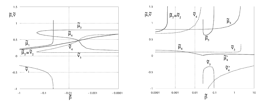
Figure 1: Five generalized de Sitter solutions ${\rm N}_{i}(\tilde{\mu}_{i},\tilde{\nu}_{i})$ ($i=1\sim 5$) with $\tilde{\mu}_{i}\geq 0$ with respect to $\tilde{\beta}$ for $\gamma<0$. Each pair of points $(\tilde{\mu}_{i},\tilde{\nu}_{i})$ with the same value of $\tilde{\beta}$ gives one solution. Number of solutions changes with the value of $\tilde{\beta}$. There is another set of time-reversed solutions ${\rm N}^{\prime}_{i}$ with $\tilde{\mu}_{i}\leq 0$.

If $\gamma>0$, we find three solutions P${}_{i}(i=1\sim 3)$ for $\beta<0$, while just one P₄ for $\beta>0$. We depict these solutions in Fig. 2 (for $\tilde{\gamma}=1$). There is no solution for $\beta=0$.

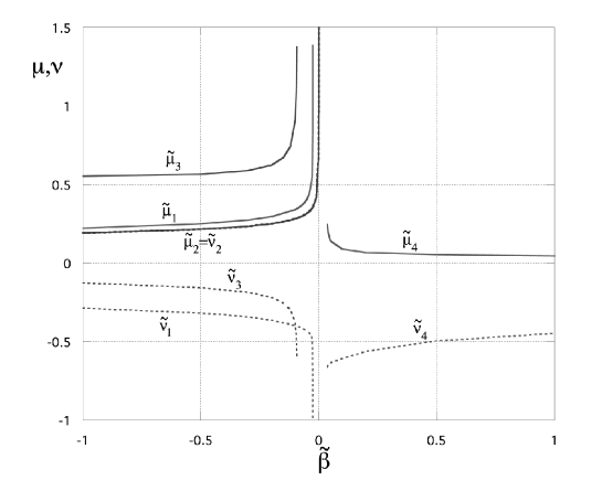
Figure 2: Four generalized de Sitter solutions ${\rm P}_{i}(\tilde{\mu}_{i},\tilde{\nu}_{i})$ ($i=1\sim 4$) with $\tilde{\mu}_{i}>0$ with respect to $\tilde{\beta}$ for $\gamma>0$. Each pair of points $(\tilde{\mu}_{i},\tilde{\nu}_{i})$ with the same value of $\tilde{\beta}$ gives one solution. Number of solutions changes with the value of $\tilde{\beta}$. There is another set of time-reversed solutions ${\rm P}^{\prime}_{i}$ with $\tilde{\mu}^{\prime}_{i}<0$. No solution exists for $\gamma>0$ and $\beta=0$.

In Table 1, we summarize their properties.

Table 1: Generalized de Sitter solutions ${\rm N}_{i}(\tilde{\mu}_{i},\tilde{\nu}_{i})$ ($i=1\sim 5$) and ${\rm P}_{i}(\tilde{\mu}_{i},\tilde{\nu}_{i})$ ($i=1\sim 4$) with $\tilde{\mu}_{i}\geq 0$ for various values of $\tilde{\beta}$ in the cases of $\tilde{\gamma}=-1$ and of $\tilde{\gamma}=1$, respectively. The solution ${\rm N}^{\prime}_{4}$ is the partner of the solution ${\rm N}_{4}$ with $\tilde{\mu}_{4}<0$, which is found when it is extended to the range of $\tilde{\beta}>0.025668$. Five eigen modes for linear perturbations are also shown. ($m$s,$n$u) means that there are $m$ stable modes and $n$ unstable modes. The solution has many stable modes if its 10-volume expansion rate ($3\tilde{\mu}+7\tilde{\nu}$) is positive.

$\gamma$	solution	property	range	stability	$3\tilde{\mu}+7\tilde{\nu}$
	${\rm N}_{1}$	$\tilde{\mu}_{1}>0>\tilde{\nu}_{1}$	$\tilde{\beta}<-0.04342$	(1s,4u)	$-$
	${\rm N}_{2}$	$\tilde{\mu}_{2}=\tilde{\nu}_{2}>0$	$\tilde{\beta}<-0.00418$	(4s,1u)	$+$
			$-0.00418<\tilde{\beta}<0.0004464$	(5s,0u)	$+$
$\tilde{\gamma}=-1$	${\rm N}_{3}$	$\tilde{\mu}_{3}>\tilde{\nu}_{3}>0$	$-0.202867<\tilde{\beta}<2.141$	(4s,1u)	$+$
	${\rm N}_{4}$	$\tilde{\mu}_{4}>\tilde{\nu}_{4}>0$	$-0.202867<\tilde{\beta}<-0.00418$	(5s,0u)	$+$
		$\tilde{\nu}_{4}>\tilde{\mu}_{4}>0$	$-0.00418<\tilde{\beta}<0.025668$	(4s,1u)	$+$
	${\rm N}^{\prime}_{4}$	$\tilde{\mu}_{4}^{\prime}>0>\tilde{\nu}_{4}^{\prime}$	$\tilde{\beta}>0.025668$	(1s,4u)	$-$
	${\rm N}_{5}$	$\tilde{\mu}_{5}>0>\tilde{\nu}_{5}$	$0.025668<\tilde{\beta}<0.09247$	(1s,4u)	$-$
	${\rm P}_{1}$	$\tilde{\mu}_{1}>0>\tilde{\nu}_{1}$		(1s,4u)	$-$
$\tilde{\gamma}=1$	${\rm P}_{2}$	$\tilde{\mu}_{2}=\tilde{\nu}_{2}>0$	$\tilde{\beta}<0$	(4s,1u)	$+$
	${\rm P}_{3}$	$\tilde{\mu}_{1}>0>\tilde{\nu}_{1}$		(4s,1u)	$+$
	${\rm P}_{4}$	$\tilde{\mu}_{1}>0>\tilde{\nu}_{1}$	$\tilde{\beta}>0$	(1s,4u)	$-$

If $\gamma=0$ and $\beta\neq 0$, we can always set $\beta$ to $-1$ if it is negative (or 1 if positive), by rescaling $\beta$, $\mu$ and $\nu$ as $\bar{\beta}=\beta/|\beta|~{}(=1~{}~{}{\rm or}~{}~{}-1)\,\,,\bar{\mu}=\mu|\beta|^{1/6}\,,\,{\rm and}\,\,\bar{\nu}=\nu|\beta|^{1/6}\,.$ We then find two solutions [$(\bar{\mu},\bar{\nu})=(0.22046,-0.28771),(0.19168,0.19168)$] for $\bar{\beta}=-1$, while just one [$(\bar{\mu},\bar{\nu})=(0.04467,-0.45111)$] for $\bar{\beta}=1$. There is no solution for $\beta=\gamma=0$.

2.2 Stability

Since the solutions obtained above correspond to fixed points in our dynamical system, we have to analyze their stabilities in order to see which solutions are more generic. We have performed a linear perturbation analysis around those fixed points. Setting $d{u}_{1}/d\tilde{t}=\tilde{\mu}_{i}+A_{i}e^{\sigma\tilde{t}}$ and $d{u}_{2}/d\tilde{t}=\tilde{\nu}_{i}+B_{i}e^{\sigma\tilde{t}}$, where $|A_{i}|,|B_{i}|\ll 1$, we write down the perturbation equations. There are five modes ($\sigma=\sigma_{a}^{(i)},~{}a=1,2,\cdots,5$) because the basic equations for $\dot{u}_{1}$ and $\dot{u}_{2}$ are two third-order differential equations plus one constraint which is second order. We show the results in Tables 1 and 2. In Table 1, we just give the number of stable and unstable modes. For example, there are one stable and four unstable modes for the solution N${}_{1}(\tilde{\mu}_{1},\tilde{\nu}_{1})$. Hence this solution may not be generic because we have many unstable modes. The M-theory has three solutions (2.1). Two solutions (${\rm N}_{2}$ and ${\rm N}_{3}$) have four stable and one unstable modes. The third solution (${\rm N}_{4}$) has five stable modes, which means that this solution is stable against linear perturbations (see Table 2).

Table 2: The eigenvalues of linear perturbation equations for $\tilde{\gamma}=-1$. We show two cases of $\tilde{\beta}$: $\tilde{\beta}=\tilde{\beta}_{S}$ and one for which we find an interesting scenario.

$\tilde{\beta}$	solution	$\tilde{\mu}_{i}$	$\tilde{\nu}_{i}$	five eigenvalues ($\sigma_{a}^{(i)},\,a=1,2,\cdots 5$)
	${\rm N}_{2}$	0.45413	0.45413	$(\,-4.5893,-4.5413,-3.6670,-0.87426,\,0.048032\,)$
$-0.0052083$	${\rm N}_{3}$	0.79802	0.10781	$(\,-4.1012,-3.1488,-2.3823,-0.76653,\,0.95268\,)$
	${\rm N}_{4}$	0.50754	0.43025	$(\,-4.5344,-4.4768,-3.6344,-0.89998,-0.057629\,)$
	${\rm N}_{1}$	0.28195	$-0.39104$	$(\,-10.2506,\,0.9457\pm 1.8339i,\,1.8914,\,12.1421\,)$
$-0.2025$	${\rm N}_{2}$	0.25005	0.25005	$(\,-5.0572,-2.5005,-1.2502\pm 5.7723i,\,2.5567\,)$
	${\rm N}_{3}$	0.71567	0.12395	$(\,-3.0268,-3.0147,-1.5073\pm 3.0912i,\,0.01217\,)$
	${\rm N}_{4}$	0.70803	0.12661	$(\,-3.01038,-2.9986,-1.5052\pm 3.2449i,-0.011765\,)$

From this stability analysis, one may conclude that the solution ${\rm N}_{4}$ is most preferable spacetime in this model. We have inflationary expansion not only in 3D external space but also in 7D internal space. The expansion rates in both spaces ($\mu,\nu$) are, however, almost the same. Hence, we would find our present world in which scales of two spaces are not so different. This solution also predicts that inflation never ends because it is stable. For a realistic cosmological model, the solution must be unstable because inflation should end. On the other hand, we also want such a solution to be rather generic which requires some sort of stability. This would be achieved if the solution contains only one unstable mode, and then the generic spacetime may first approach this solution and gradually leave it, recovering the present Friedmann universe, where we expect the higher order terms become irrelevant. We find that the solution ${\rm N}_{3}$ may give one possible candidate for such a model. We now discuss a new scenario obtained from this solution in the next section.

3 A Scenario for Large Extra Dimensions

Let us discuss the evolution of the early universe for the solution ${\rm N}_{3}(\tilde{\mu}_{3},\tilde{\nu}_{3})=(0.79802,0.10781)$ with $\beta=\beta_{S}$. The scale factor of the external space expands as $e^{0.79802\tilde{t}}$. For a successful inflation (resolution of flatness and horizon problems), we need at least 60 e-foldings. Let us assume that inflation will end after 60 e-foldings, i.e. $0.79802\tilde{t}_{\rm end}\approx 60$. The inflation will end because ${\rm N}_{3}$ has one unstable mode. During inflation the internal space also expands exponentially. When inflation ends, its scale becomes $e^{0.10781\tilde{t}_{\rm end}}\approx 4000$ times larger than the initial scale length, which we assume to be the 11D Planck length ($m_{11}^{-1}$). After inflation, if the internal space settles down to static one, the present radius of extra dimensions is $R_{0}\sim 4000m_{11}^{-1}$. Since this is slightly larger than the fundamental scale length, we may adopt the model of large extra dimensions, which was first proposed as a brane world by Arkani-Hamed et al. [15]. In this model, the 4D Planck mass is given by

$$m_{4}^{2}\sim R_{0}^{7}m_{11}^{9}\sim 1.6\times 10^{25}m_{11}^{2}\,.$$ (14)

We then find

$$m_{11}\sim 2.5\times 10^{-13}m_{4}\sim 600{\rm TeV}\,.$$ (15)

This is our fundamental energy scale. The present scale of extra dimensions is $4000m_{11}^{-1}\sim 7$ TeV^-1, which could be observed in the accelerators of next generation.

We can also put our argument in a different way. Suppose that the e-folding of inflation is $N$, which is related to the stability of the solution. The 3-space expands as $e^{N}=e^{\tilde{\mu}\tilde{t}_{\rm end}}$, while the internal space becomes $e^{\tilde{\nu}\tilde{t}_{\rm end}}$ times larger. It follows from Eq. (14) that

$$m_{11}\sim e^{-{7\nu\over 2\mu}N}m_{4}\,.$$ (16)

Since $m_{11}\,\mbox{\raisebox{-4.30554pt}{$\stackrel{{\scriptstyle\textstyle>}}{{\textstyle\sim}}$}}\,1$ TeV from the present experiments, we have a constraint on the e-folding as $N\,\mbox{\raisebox{-4.30554pt}{$\stackrel{{\scriptstyle\textstyle<}}{{\textstyle\sim}}$}}\,10\mu/\nu$. Then if we have TeV gravity and $\mu\,\mbox{\raisebox{-4.30554pt}{$\stackrel{{\scriptstyle\textstyle>}}{{\textstyle\sim}}$}}\,6\nu(>0)$, we can naturally explain why the e-folding of inflation is about 60 and but not so large. Recall that the solution ${\rm N}_{3}$ with $\gamma<0$ gives $5.72<\mu/\nu<10.22$ (corresponding to $57\,\mbox{\raisebox{-4.30554pt}{$\stackrel{{\scriptstyle\textstyle<}}{{\textstyle\sim}}$}}\,N\,\mbox{\raisebox{-4.30554pt}{$\stackrel{{\scriptstyle\textstyle<}}{{\textstyle\sim}}$}}\,102$) for any value of $\beta$.

Although the above solution ${\rm N}_{3}$ has one unstable mode, its eigenvalue $\sigma_{5}^{(3)}$ is of the same order of magnitude as other eigenvalues of stable modes as seen from Table 2 and is a little too large to give enough expansion. If the eigenvalue of the unstable mode is much smaller than those of other four stable modes, a preferable generalized de Sitter solution is naturally obtained for a wide range of initial conditions. Can we find such a possibility in superstrings or M-theory? We note that our starting Lagrangian has some ambiguity, that is, the fourth-order correction term $S_{4}$ is fixed up to the Ricci curvature tensors. If we include correction terms including the Ricci curvature tensors, our basic equations will be modified. We might effectively take their effect into account by changing the value of our coefficient $\gamma$ or $\tilde{\beta}$ after the rescaling. Thus we may look for a preferable solution by changing $\tilde{\beta}$. We find that the solution ${\rm N}_{3}$ with $\tilde{\beta}=-0.2025$ shows interesting behaviors (see Table 2). Four modes are stable and the eigenvalue of one unstable mode is very small, i.e. $\sigma^{(3)}_{5}=0.01217$. Then the time scale in which this unstable mode becomes important is evaluated as $\tilde{t}_{\rm us}\approx(\sigma^{(3)}_{5})^{-1}\sim 82$. Since the eigenvalues of other stable modes are of order unity, for a wide range of initial conditions, general solutions first approach the solution ${\rm N}_{3}$, which gives us an inflationary stage, after one dynamical time ($\tilde{t}\sim O(1)$). The unstable mode becomes important at $\tilde{t}\sim\tilde{t}_{\rm us}$, and then the inflation ends. We may have enough e-folding time of inflation ($N\approx\tilde{\mu}_{3}\tilde{t}_{\rm us}\sim 58.8$). In this case, we find $m_{11}\sim 3.3\times 10^{-16}m_{4}\sim 0.8$ TeV, which gives us a TeV gravity theory.

Although we find a successful exponential expansion and its natural end, this is not enough for a successful inflation. We need a reheating mechanism and have to create a density fluctuation as a seed of cosmic structure. A gravitational particle creation may provide a reheating mechanism [17], because the background spacetime is time dependent and there might have some oscillation when the internal space settles down to static one which is required to explain our present universe. As for a density perturbation, our model may not give a good scenario because our energy scale is $|\gamma|^{-1/6}\sim 5m_{11}\sim 4$ TeV. We have to invoke other mechanism for density perturbations such as a curvaton model [18].

References

- [1] For recent WMAP data, see http://map.gsfc.nasa.gov/.
- [2] P.K. Townsend and N.M.R. Wohlfarth, Phys. Rev. Lett. 91 (2003) 061302, hep-th/0303097.
-
[3]
N. Ohta, Phys. Rev. Lett. 91 (2003) 061303, hep-th/0303238;
N. Ohta, Prog. Theor. Phys. 110 (2003) 269, hep-th/0304172. -
[4]
C.-M. Chen, D.V. Gal’tsov and M. Gutperle, Phys. Rev. D 66 (2002) 024043,
hep-th/0204071;
N. Ohta, Phys. Lett. B 558 (2003) 213, hep-th/0301095. -
[5]
M. Kruczenski, R.C. Meyers and A.W. Peet, JHEP 0205 (2002) 039,
hep-th/0204144;
V.D. Ivashchuk, Class. Quant. Grav. 20 (2003) 261, hep-th/0208101. See also H. Lu, S. Mukherji, C.N. Pope and K.W. Xu, Phys. Rev. D 55 (1997) 7935. -
[6]
C.P. Burgess, P. Martineau, F. Quevedo, G. Tasinato and I. Zavala,
JHEP 0303 (2003) 050, hep-th/0301122;
A. Buchel and J. Walcher, JHEP 0305 (2003) 069, hep-th/0305055. - [7] N.M.R. Wohlfarth, Phys. Lett. B B563 (2003) 1, hep-th/0304089.
-
[8]
S. Roy, Phys. Lett. B 567 (2003) 322, hep-th/0304084;
R. Emparan and J. Garriga, JHEP 0305 (2003) 028, hep-th/0304124;
C.-M. Chen, P.M. Ho, I. Neupane and J.E. Wang, JHEP 0307 (2003) 017, hep-th/0304177;
M. Gutperle, R. Kallosh and A. Linde, JCAP 0307 (2003) 001, hep-th/0304225. - [9] C.-M. Chen, P.M. Ho, I. Neupane, N. Ohta and J.E. Wang, JHEP 0310 (2003) 058, hep-th/0306291.
-
[10]
A.A. Starobinski, Phys. Lett. B 91 (1980) 99;
K. Maeda, Phys. Lett. B 166 (1986) 59;
J. Ellis, N. Kaloper, K.A. Olive and J. Yokoyama, Phys. Rev. D 59 (1999) 103503, hep-ph/9807482. - [11] See, e.g. Modern Kaluza-Klein Theories, Chap. VI, ed. by T. Appelquist, A. Chodos and P.G.O. Freund (1987, Addison-Wesley).
- [12] H. Ishihara, Phys. Lett. B 179 (1986) 217.
- [13] N. Deruelle and L. Fariña-Busto, Phys. Rev. D 41 (1990) 3696.
-
[14]
A. Tseytlin, Nucl. Phys. B 584 (2000) 233, hep-th/0005072;
K. Becker and M. Becker, JHEP 0107 (2001) 038, hep-th/0107044. -
[15]
N. Arkani-Hamed, S. Dimopoulos and G. Dvali, Phys. Lett. B 429 (1998)
263, hep-ph/9803315;
I. Antoniadis, N. Arkani-Hamed, S. Dimopoulos and G.R. Dvali, Phys. Lett. B 436 (1998) 257, hep-ph/9804398. - [16] K. Maeda and N. Ohta, in preparation.
-
[17]
L. H. Ford, Phys. Rev. D 35 (1987) 2955;
B. Spokoiny, Phys. Lett. B 315 (1993) 40. -
[18]
D.H. Lyth and D. Wands, Phys. Lett. B 524 (2002) 5, hep-ph/0110002;
T. Moroi and T. Takahashi, Phys. Lett. B 522 (2001) 215, hep-ph/0110096.