The static potential in QED₃ with non-minimal coupling

Abstract

Here we study the effect of the non-minimal coupling $j^{\mu}\epsilon_{\mu\nu\alpha}\partial^{\nu}A^{\alpha}$ on the static potential in multiflavor QED₃. Both cases of four and two components fermions are studied separately at leading order in the $1/N$ expansion. Although a non-local Chern-Simons term appears, in the four components case the photon is still massless leading to a confining logarithmic potential similar to the classical one. In the two components case, as expected, the parity breaking fermion mass term generates a traditional Chern-Simons term which makes the photon massive and we have a screening potential which vanishes at large inter-charge distance. The extra non-minimal couplings have no important influence on the static potential at large inter-charge distances. However, interesting effects show up at finite distances. In particular, for strong enough non-minimal coupling we may have a new massive pole in the photon propagator while in the opposite limit there may be no poles at all in the irreducible case. We also found that, in general, the non-minimal couplings lead to a finite range repulsive force between charges of opposite signs.

PACS-No.: 11.15.Bt , 11.15.-q

1 Introduction

One of the most intriguing and longstanding problems in high energy physics is a complete understanding of the mechanism of color confinement in 4D QCD. Several models and techniques have been used to gain a deeper insight on this problem. In particular, supersymmetry has been used in the four dimensional theory treated in [1] while bosonization has played an important role in the analysis of screening/confinement issues in $D=2$ models [2, 3, 4]. Those models have in common that it is necessary to have massive fermions to produce confinement. This happens also in parity preserving QED in $2+1$ dimensions [5] which will be treated in this work altogether with the parity breaking (2 components fermions) case. Technically, although bosonization is not so well developed in $D>2\,$, we can always integrate perturbatively over the fermionic fields (see [6, 7, 8, 9, 10, 11])and derive an effective bosonic action for the vector field. Such effective action is in general non-local even in $D=2$ [3]. From this bosonic action we have an expression for the vector boson propagator including vacuum polarization or even higher order effects. A detailed analysis of the analytic structure of the propagator already reveals, qualitatively, the large distance behavior of the interaction. In fact, even in other non-equivalent approaches to study confinement, like Schwinger-Dyson equations, see e.g. [5], the infrared properties of the vector field propagator including vacuum polarization corrections play a key role. Here we formally minimize the effective action and calculate the energy $V(L)$ between two static charges separated by a distance $\,L\,$ by solving the resulting differential equation. Basically, this is the route followed in [12, 13, 14] in the case of $QED_{3}$ with two components fermions (irreducible QED). In that case an usual, linear in momentum, Chern-Simons term is generated which makes the photon massive [15] leading to a screening potential in opposition to what happens classically. In [16] we have added a quartic interaction of Thirring type ${\cal L}_{Th}=g^{2}(\bar{\psi}^{i}\gamma^{\mu}\psi^{i})^{2}/N$ and checked that the screening scenario prevails again in multiflavor irreducible $QED_{3}$ , at least at leading order in $1/N$, see also [17, 18]. By passing, we noticed in [16] that in the case of four components fermions with a parity symmetric mass term, henceforth called reducible QED, the vacuum polarization is not strong enough to change the classical picture and the potential remains logarithmic confining at leading order in $1/N$. In all the works [12, 13, 14, 16] the fermions were minimally coupled to the eletromagnetic potential. The aim of this work is to analyze the effect on the screening/confining scenario of adding a non-minimal coupling term which preserves gauge symmetry and it is rather natural in $2+1$ dimensions, namely, we add $F_{\mu}j^{\mu}=\epsilon_{\mu\nu\alpha}\partial^{\nu}A^{\alpha}j^{\mu}$ to the minimally coupled QED action. In the irreducible case this extra coupling corresponds to a magnetic moment interaction of the Pauli type. Such non-minimal coupling has been considere before in [19, 20, 21, 22, 23, 24] in different contexts. It seems to lead to anyons without the need of a topological Chern-Simons term as argued in [21, 24] and [22] ( see however [23]). Our interest lies in the fact that $F_{\mu}j^{\mu}$ breaks parity explicitly and the presence of parity breaking terms is very important for the pole structure of the photon propagator.

We start with the partition function:

$$Z = \int\mathcal{D}A_{\mu}\,\prod_{r=1}^{N}\mathcal{D}\psi_{r}\,\mathcal{D}\bar{\psi}_{r}\,exp\left\{i\,\int\,d^{3}x\,\,\left[-\frac{1}{4}\,F_{\mu\nu}^{2}\,+\frac{\zeta}{2}\left(\partial_{\mu}A^{\mu}\right)^{2}\right.\right.$$ (1)

$$\left.\left.+\,\bar{\psi}_{r}\,(i\,\partial\!\!\!/\,-\,m\,-\,\frac{e}{\sqrt{N}}\,A\!\!\!/-\frac{\gamma}{\sqrt{N}}\,F\!\!\!\!/)\psi_{r}+(A_{\nu}+\mu F_{\nu})\,j_{\rm ext}^{\nu}\,\right]\right\}\ ,$$

where $F_{\mu}=\epsilon_{\mu\nu\alpha}\partial^{\nu}A^{\alpha}$. Summation over repeated flavor index $r$ ($r=1,2,...,N$) is assumed. The constant $\mu$ represents the magnetic moment of the static charge while $\gamma$ sets the strength of the dynamical fermions non-minimal coupling. Those couplings have mass dimension $-1$ and $-1/2$ respectively. The external current is generated by a static charge at the point $(x_{1},x_{2})=(L/2,0)$, i.e.,

$$j_{\rm ext}^{\nu}=Q\delta(x_{2})\delta({x_{1}}-{\frac{L}{2}})\delta^{\nu 0}$$ (2)

Integrating over the fermions we have an effective action for the photons:

$$Z = \int\mathcal{D}A_{\mu}exp\left\{\,i\,\int\,d^{3}x\,\left[\,-\frac{1}{4}\,F_{\mu\nu}^{2}\,+\,\frac{\zeta}{2}\left(\partial_{\mu}A^{\mu}\right)^{2}+(A_{\nu}+\mu F_{\nu})\,j_{\rm ext}^{\nu}\right]+\right.$$ (3)

$$\left.\qquad\qquad\qquad\qquad\quad+\quad N\,{\rm Tr}\,\ln\left[i\partial\!\!\!/\,-\,m\,-\,{\frac{(e\,A\!\!\!/\,+\,\gamma\,F\!\!\!\!/)}{\sqrt{N}}}\,\right]\,\right\}$$

$$= \int\mathcal{D}A_{\mu}exp\left\{+\,i\,\int\,d^{3}x\,\left[\,-\frac{1}{4}\,F_{\mu\nu}^{2}\,+\,\frac{\zeta}{2}\left(\partial_{\mu}A^{\mu}\right)^{2}+(A_{\nu}+\mu F_{\nu})\,j_{\rm ext}^{\nu}\right]\right.$$

$$\left.\qquad+\,\,\int\frac{d^{3}k}{2(2\pi)^{3}}\left[e\tilde{A}^{\mu}(k)+\gamma{\tilde{F}}^{\mu}(k)\right]\Pi_{\mu\nu}\left[e\tilde{A}^{\nu}(-k)+\gamma{\tilde{F}}^{\nu}(-k)\right]+{\cal O}(1/N)\right\}$$

The logarithm has been evaluated perturbatively in $1/N$. Due to Furry’s theorem, only even number of vertices contribute. Since each vertex is of order $1/\sqrt{N}$ the leading contribution with two vertices, that corresponds to the vacuum polarization diagram, will be $N$-independent due to the trace over the internal femion lines. The next to leading contribution with four vertices is of order $1/N$ and will be neglected henceforth. In particular, our results will be exact for $N\to\infty$. The quantities ${\tilde{A}}_{\mu}(k)$ and ${\tilde{F}}_{\mu}(k)$ represent the Fourier transformations of $A_{\mu}(x)$ and ${F}_{\mu}(x)$ respectively and $\Pi^{\mu\nu}$ is the polarization tensor:

$$\Pi^{\mu\nu}(k)=i\int\;\frac{d^{3}p}{(2\pi)^{3}}\;tr\left[\frac{1}{p\!\!\!/-m+i\epsilon}\gamma^{\mu}\frac{1}{(p\!\!\!/+k\!\!\!/)-m+i\epsilon}\gamma^{\nu}\right]$$ (4)

The calculation of $\Pi^{\mu\nu}$ is regularization dependent. Using dimensional regularization which preserves gauge symmetry and does not add any artificial parity breaking term, we have :

$$\Pi_{\mu\nu}(k)\,=\,\frac{f_{2}}{16\pi m}(k^{2}g_{\mu\nu}-k_{\mu}k_{\nu})+\frac{if_{1}}{8\pi}\epsilon_{\mu\nu\alpha}k^{\alpha}$$

Defining $z=k^{2}/(4m^{2})$, in the case of two components fermions, in the range $0\leq z<1$, we have

$$f_{1}\, = -\frac{1}{\sqrt{z}}\ln\frac{1+\sqrt{z}}{1-\sqrt{z}}$$

$$f_{2}\, = \frac{1}{z}\left(1+\frac{1+z}{2}f_{1}\right)$$ (5)

While for $\,z\leq 0\,$ ,

$$\tilde{f}_{1}\, = -\frac{2}{\sqrt{-z}}\arctan\sqrt{-z}$$

$$\tilde{f}_{2}\, = -\frac{1}{z}\left(1+\frac{1-z}{2}\tilde{f}_{1}\right)$$ (6)

Above the pair creation threshold $z>1$ the effective action will develop an imaginary part which we are not interested in and do not write it down here. In the simpler case of four components fermions we have instead: $f_{1}\to 0\,,\,f_{2}\to 2f_{2}$ ($\,\tilde{f}_{1}\to 0\,,\,\tilde{f}_{2}\to 2\tilde{f}_{2}\,$).

From (3) we can read off the effective action:

$$S_{\rm eff}\,=\,\int d^{3}x\,d^{3}y\left[A^{\mu}(x)\frac{D^{-1}_{\mu\nu}(x,y)}{2}A^{\nu}(y)+(A_{\nu}+\mu F_{\nu})j_{ext}^{\nu}\delta^{(3)}(x-y)\right]$$ (7)

Where $D^{-1}_{\mu\nu}(x,y)$ is the inverse of the propagator in the space-time. Minimizing the effective action we deduce:

$$A_{\beta}(y)\, = \,-\int d^{3}x\,D_{\beta\alpha}(y,x)\left[j^{\alpha}_{\rm ext}(x)+\mu\,\epsilon^{\alpha}_{\nu\gamma}\partial^{\nu}j^{\gamma}_{\rm ext}(x)\right]$$ (8)

$$= \,-\int\frac{d^{3}k}{(2\pi)^{3}}\,\tilde{D}_{\beta\alpha}(k)\int d^{3}xe^{ik\cdot(y-x)}\left[j^{\alpha}_{\rm ext}(x)+\mu\,\epsilon^{\alpha}_{\nu\gamma}\partial^{\nu}j^{\gamma}_{\rm ext}(x)\right]$$

Introducing the dimensionless couplings:

$$c_{1}\, = \,e^{2}/16\pi m$$ (9)

$$c_{2}\, = \,e\gamma/4\pi$$ (10)

We can write the propagator in momentum space as:

$$\tilde{D}_{\mu\nu}(k)\,=\,a\,g_{\mu\nu}+b\left(g_{\mu\nu}-\frac{k_{\mu}k_{\nu}}{k^{2}}\right)+c\,\epsilon_{\mu\nu\alpha}k^{\alpha}$$ (11)

For $0\leq z<1$ the coefficients are given by

$$a\, = \,\frac{1}{4m^{2}\zeta z}\,$$ (12)

$$a+b\, = \,\frac{c_{1}}{8m^{2}}\frac{D_{+}+D_{-}}{\sqrt{z}D_{+}D_{-}}$$ (13)

$$c\, = \,-\frac{ic_{1}}{16m^{3}z}\frac{D_{+}-D_{-}}{D_{+}D_{-}}$$ (14)

$$D_{\pm} = \,(c_{1}\pm\sqrt{z}c_{2})^{2}G_{\pm}-\sqrt{z}c_{1}\quad;\quad G_{\pm}\,=\,\sqrt{z}f_{2}\pm f_{1}$$ (15)

while for $z\leq 0$,

$$\tilde{a}\, = \,-\frac{1}{4m^{2}\zeta z}\,$$ (16)

$$\tilde{a}+\tilde{b}\, = \,\frac{c_{1}}{4m^{2}}\frac{(c_{1}^{2}+zc_{2}^{2})^{2}\left[(c_{1}^{2}-zc_{2}^{2})\tilde{f}_{2}-c_{1}(1+2c_{2}\tilde{f}_{1})\right]}{A^{2}+z\,B^{2}}$$ (17)

$$\tilde{c}\, = \,i\frac{c_{1}(c_{1}^{2}+zc_{2}^{2})^{2}\left[(c_{1}^{2}-zc_{2}^{2})\tilde{f}_{1}-2c_{1}c_{2}\tilde{f}_{2}z\right]}{16m^{3}z(A^{2}+z\,B^{2})}$$ (18)

$$A\, = \,(c_{1}^{2}+zc_{2}^{2})^{2}\tilde{f}_{1}-2zc_{1}^{2}c_{2}\quad;\quad B\,=\,(c_{1}^{2}+zc_{2}^{2})^{2}\tilde{f}_{2}-c_{1}(c_{1}^{2}-zc_{2}^{2})$$ (19)

Returning to the calculation of (8), since the external current is time independent the integral $\int dx_{0}e^{-ik_{0}x_{0}}=2\pi\delta(k_{0})$ allows us to exactly integrate over $k_{0}$ which amounts to set $k^{\mu}k_{\mu}=-k_{1}^{2}-k_{2}^{2}\equiv-k^{2}<0$ inside (8). We can integrate over $dx_{1}dx_{2}$ using $\delta(x_{1}-L/2)\delta(x_{2})$. The integral over the angle part of $d^{2}k=kdkd\theta$ gives rise to a $J_{0}$ Bessel function. Thus, we are left with the integral over $k=\sqrt{k_{1}^{2}+k_{2}^{2}}$. Placing the negative charge $-Q$ at $(x_{1},x_{2})=(-L/2,0)$ we finally have the energy of the pair separated by a distance $L$:

$$V(L) \,=\, \,-Q\,A_{0}(y_{1}=-L/2,y_{2}=0)$$ (20)

$$\,=\, -\frac{Q^{2}}{2\pi}\int_{0}^{\infty}dk\,k\,\left({\tilde{a}}+\tilde{b}+i\mu\tilde{c}k^{2}\right)J_{0}(kL)$$

The last formula shows that the non-minimal $\mu$-term can only contribute to $V(L)$ if the photon propagator contains a parity breaking piece ($\tilde{c}\neq 0$).

In the next two sections we split the discussion into the cases of four (reducible) and two (irreducible) components fermions.

2 Reducible QED ($4\times 4$ representation )

2.1 Effective action and pole analysis

In this case, the inclusion of vacuum polarization effects leads to the following non-local Lagrangian density:

$${\cal L}_{eff}\, = \,\frac{\zeta(\partial_{\mu}A^{\mu})^{2}}{2}\,-\frac{e\gamma}{4\pi m}\epsilon_{\mu\nu\alpha}A^{\mu}\Box f_{2}\partial^{\nu}A^{\alpha}$$ (21)

$$- \frac{F_{\mu\nu}}{4}\left[1-\left(\frac{e^{2}-4\gamma^{2}\Box}{8\pi m}\right)f_{2}\right]F^{\mu\nu}+(A_{\nu}+\mu F_{\nu})\,j_{\rm ext}^{\nu}$$

Where $f_{2}=f_{2}(-\Box/4m^{2})\,$ is given in (5) and (6). Notice that, within dimensional regularization $\Pi_{\mu\nu}$ is parity symmetric ($f_{1}=0$ ) but still, as a consequence of the parity breaking non-minimal coupling there appears a non-local Chern-Simons term in (21) which breaks parity .

Concerning the pole structure of the propagator, setting $f_{1}\to 0$ and $f_{2}\to 2f_{2}$ in (15) we obtain $D_{+}D_{-}=z\left[2(c_{1}+\sqrt{z}c_{2})^{2}f_{2}-c_{1}\right]\left[2(c_{1}-\sqrt{z}c_{2})^{2}f_{2}-c_{1}\right]$. Since $f_{2}\leq-4/3\,$ and $c_{1}>0\,$ it is clear that the only pole we have appears at the origin $\,z=0\,$. Therefore, quite surprisingly, the non-local Chern-Simons term in (21) is not able to make the photon massive like its local counterpart. Although parity is broken, the photon is still massless.

2.2 V(L)

For the calculation of $V(L)$ it is important to find the singularities of (17) and (18). By inspection we observe that the denominators of $\tilde{a}+\tilde{b}$ and $\tilde{c}$ can only vanish either for $z=0$ or $A=0=B$. However, since $\tilde{f}_{1}=0$ it is clear from (19) that the later possibility also requires $z=0$. Thus, we conclude that the expression to be integrated in $V(L)$ contains only one singular point which is a simple pole at $z=0$. By passing, this implies that we have no tachyons in the reducible case.

Substituting (17) and (18), with $\tilde{f}_{1}\to 0$ and $\tilde{f}_{2}\to 2\tilde{f}_{2}$, in (20) we derive, after trivial manipulations:

$$V(L)\,=\,\int_{0}^{\infty}\frac{dk}{k}J_{0}(kL)G(k)$$ (22)

Where, besides the Bessel function $J_{0}$, we have

$$G(k)\,=\,-\frac{Q^{2}c_{1}}{2\pi}\frac{c_{1}(1-2c_{1}\tilde{f}_{2})+2c_{2}z\tilde{f}_{2}(c_{2}-2\mu c_{1})}{(2zc_{2}^{2}\tilde{f}_{2}+c_{1})^{2}-4c_{1}^{3}\tilde{f}_{2}(1-c_{1}\tilde{f}_{2})}$$ (23)

Note that $\tilde{f}_{2}\leq-4/3$ which confirms that $k=0$ is the only singularity in (22). The way it stands, the integral in (22) does not exist since $J_{0}(0)=1$ and $G(0)=-3Q^{2}/[2\pi(3+8c_{1})]$ are both finite and non-vanishing . In order to eliminate the infrared divergence at $k=0$ we make a subtraction, namely :

$$V(L)-V(L_{0})\,=\,\lim_{x\to 0}\int_{x}^{\infty}\frac{dk}{k}[J_{0}(kL)-J_{0}(kL_{0})]G(k)$$ (24)

We can recover the classical result by taking $c_{1}=0=c_{2}$ which gives $G(k)=-Q^{2}/2\pi$. In this case the integral (24) can be easily calculated furnishing the well known confining potential:

$$V(L)-V(L_{0})\,=\,\frac{Q^{2}}{2\pi}\ln\frac{L}{L_{0}}$$ (25)

However, in the general case we have to calculate the integral numerically. One exception is the limit $m\to\infty$. First, notice that if we simply take $m\to\infty$ the effective action (21) becomes the classical Maxwell action at leading order and all quantum information is lost. On the other hand, if we take $m\to\infty$ while keeping $c_{1}$ and $c_{2}$ finite the effective action (21) becomes:

$${\cal L}_{eff}\,=\,-\frac{1}{4}\left(1+\frac{8c_{1}}{3}\right)F_{\mu\nu}F^{\mu\nu}+\frac{\zeta(\partial_{\mu}A^{\mu})^{2}}{2}+(A_{\nu}+\mu F_{\nu})\,j_{\rm ext}^{\nu}+{\cal O}\left(\frac{1}{m}\right)$$ (26)

Correspondingly, this amounts to substitute $G(k)$ by $G(0)$ in (24). Therefore we have :

$$V(L)-V(L_{0})\, = \,-G(0)\ln\left(L/L_{0}\right)\,=\,\frac{3Q^{2}}{[2\pi(3+8c_{1})]}\log\left(L/L_{0}\right)$$ (27)

$$= \,\frac{Q_{\rm scr.}^{2}}{2\pi}\log\left(L/L_{0}\right)$$

Where

$$Q_{\rm scr.}\,=\,\frac{Q}{\left[1+\frac{e^{2}}{6\pi m}\right]^{1/2}}$$ (28)

Thus, we see that at leading order in $1/m$ the vacuum polarization has a mild effect on the classical static potential. It leads to a screening of the static charges but it is not strong enough to change the confining nature of the potential. In particular, the non-minimal couplings introduced by the constants $\gamma\,$ and $\,\mu$ have no influence at all. In fact, this is not surprising since we are keeping $c_{1}$ and $c_{2}$ fixed and taking $m\to\infty$ which corresponds to $e\sim\sqrt{m}$ and $\gamma\sim 1/\sqrt{m}$. This is a situation where the minimal coupling certainly prevails against the non-minimal one.

In order to clearly outline the effect of the non-minimal coupling we must keep all parameters $(c_{1},c_{2},m)$ finite and calculate $V(L)$ numerically. Our results for the reducible case are shown in figure 1 (pure QED) and figure 2 (non-minimally coupled QED).

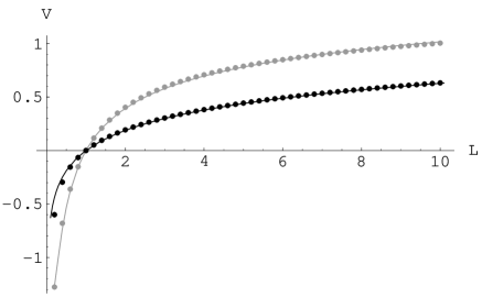
Figure 1: The static potential for pure $QED_{3}$ (reducible) with $(c_{1},c_{2},\mu)=(1,0,0)$ and $m=1$ (dark dots), $m=0.1$ (light dots). The dark solid curve corresponds to the $m\to\infty$ result $(3/11)\ln L$ and the light solid one to the fit $(3/11)\ln L-0.48/L+0.046/L^{2}+0.44$.

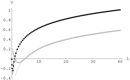
Figure 2: The static potential for $QED_{3}$ (reducible) with non-minimal coupling $(c_{1},c_{2},\mu)=(1,0.5,0)$ and $m=1$ (dark dots), $m=0.1$ (light dots). The dark solid curve corresponds to the $m\to\infty$ result $(3/11)Log[L]$ and the light solid one to the fit $(3/11)\ln L-0.42$.

Fixing $c_{1}=1$ we see that in both figures the value $m=1$ is already very close to the $m\to\infty$ case. This could also be interpreted as a confirmation of our numerical integration which is rather trick due to the oscillations of the Bessel function. The remarkable effect of the non-minimal coupling is a repulsive force in a finite range $0\leq L\leq L_{min}$. Numerically we have noticed that $L_{min}\sim 1/m$. In particular, in figure 2 $L_{min}\sim 2.5$ and $0.25$ respectively for $m=0.1$ and $m=1$. The effect produced by $c_{2}\neq 0$ and $\mu=0$ can be similarly caused by making $\mu\neq 0$ and $c_{2}=0$. Furthermore, they can also compete such that the repulsive force can be turned off if we set $\mu$ and $c_{2}$ accordingly. The same happens in the irreducible case (next section) and the figures we have are similar (for small $L$) to the figures 3-5. Therefore we skip them. The logarithmic fittings in figures 1 and 2 are in agreement with the analytic result derived in the appendix of [30] for pure QED (reducible), namely, $V(L)=-G(0)\ln L+{\rm constant}+h(L)$ where $h(L)$ should fall off at least as fast as $1/L$ as $L\to\infty$. In summary, the new couplings $\gamma$ and $\mu$ can only play a role at finite $L$. The point is that if we use a $4\times 4$ representation only a higher order Chern-Simons term will be generated due to the parity breaking non-minimal coupling but as $k\to 0$ this term will be negligible if compared to a Maxwell term and the photon remains massless as it is classically. Consequently, the origin $k=0$ will dominate the calculation of $V(L)$. Around that region the higher momenta coupling terms which multiply $\gamma$ and $\mu$ can be dropped.

3 Irreducible QED ($2\times 2$ representation )

3.1 Effective action and pole analysis

Due to the parity breaking term of $\Pi_{\mu\nu}\,$ the effective action now is more complicated:

$${\cal L}_{eff}\, = \,\frac{\zeta(\partial_{\mu}A^{\mu})^{2}}{2}\,-\epsilon_{\mu\nu\alpha}A^{\mu}\left[\frac{e\gamma\Box f_{2}}{8\pi m}+\left(\frac{e^{2}-4\gamma^{2}\Box}{16\pi}\right)f_{1}\right]\partial^{\nu}A^{\alpha}$$ (29)

$$- \frac{F_{\mu\nu}}{4}\left[1-\left(\frac{e^{2}-4\gamma^{2}\Box}{16\pi m}\right)f_{2}-\frac{e\gamma}{2\pi}f_{1}\right]F^{\mu\nu}+(A_{\nu}+\mu F_{\nu})\,j_{\rm ext}^{\nu}$$

Where $f_{2}=f_{2}(-\Box/4m^{2})$ and $f_{1}=f_{1}(-\Box/4m^{2})$ are given in (5) and (6) .

For finite fermion mass the analysis of the singularities of the photon propagator is much more involved. First of all, the pole at $z=0$ in (14),which also appears in the local Maxwell Chern-Simons theory, is not a physical one. In particular, it disappears if we look at the gauge invariant propagator $<F_{\mu}(k)F_{\nu}(-k)>$. Thus, the physical poles can only come from either $D_{+}=0$ or $D_{-}=0$. Since $G_{+}\leq-2$ the first possibility is ruled out, see (15). Therefore, we have to examine the equation $D_{-}=(c_{1}-\sqrt{z}c_{2})^{2}G_{-}-\sqrt{z}c_{1}\quad=0$ with $G_{-}$ being a monotonically decreasing function in the range $1\leq G_{-}\leq 2$. We have not been able to find an analytical solution to that equation but we have made a rather detailed analysis on the number of poles ($n$) in the region $0\leq k^{2}<4m^{2}$ according to different coupling values. One can show analytically that,

$$c_{2}\,>c_{1}+\sqrt{c_{1}}\quad \rightarrow \quad n=2$$ (30)

$$c_{2}\,<\,-1/4\quad \rightarrow \quad n=0$$ (31)

$$-1/4\,\leq\,c_{2}\,<\,c_{1}-\sqrt{c_{1}}\quad \rightarrow \quad n=0\quad{\rm if}\quad c_{1}\,\geq\,1$$ (32)

$$c_{1}-\sqrt{c_{1}}\,<\,c_{2}\,<\,c_{1}+\sqrt{c_{1}}\quad \rightarrow \quad n=1\quad{\rm if}\quad c_{1}\,\geq\,1$$ (33)

$$0\,<\,c_{2}\,<\,c_{1}+\sqrt{c_{1}}\quad \rightarrow \quad n=1\quad{\rm if}\quad c_{1}\,\leq\,1$$ (34)

The missing region $c_{1}<1$ and $-1/4\leq c_{2}<0\,$ is rather awkward and only numerical results have been obtained. In particular, besides $n=0,1,2$ poles we also found it possible to have $n=3$ poles if the QED coupling is very small $0<c_{1}<0.041$.

It is remarkable that for $c_{2}>0$, the poles follow basically the same pattern [16] of QED with a Thirring term ${\cal L}_{Th}=g^{2}(\bar{\psi}^{i}\gamma^{\mu}\psi^{i})^{2}/N$ [16] with the Pauli coupling $\gamma$ playing the role of $g$. Namely, for strong enough Pauli coupling, when compared to the QED coupling , a new pole appears besides the one we have in pure QED. If $\gamma$ is reduced this extra pole disappears. Besides, for very strong QED coupling we may have no real poles at all. That also happens in pure QED as we remarked in [16]. It is tempting to ascribe those similarities with the QED plus Thirring case to the fact that both couplings $g$ and $\gamma$ have the same mass dimension $m^{-1/2}$.

Finally, we stress that it is impossible to have a massless photon in the $2\times 2$ representation whatever value we choose for $c_{1}$ and $c_{2}$.

3.2 V(L)

Now the integral we need to evaluate is:

$$V(L)-V(L_{0})\,=\,\lim_{x\to 0}\int_{x}^{\infty}dk\,k\,[J_{0}(kL)-J_{0}(kL_{0})]H(k)$$ (35)

Where,

$$H(k)\,=\,-\frac{Q^{2}\,c_{1}}{8\pi m^{2}}\,\frac{(c_{1}^{2}+zc_{2}^{2})^{2}\left[(c_{1}^{2}-zc_{2}^{2}+2\mu mc_{1}c_{2}z)f_{2}+2c_{1}c_{2}f_{1}-\mu m(c_{1}^{2}-zc_{2}^{2})f_{1}-c_{1}\right]}{[(c_{1}^{2}+zc_{2}^{2})^{2}\tilde{f}_{1}-2zc_{1}^{2}c_{2}]^{2}+z[(c_{1}^{2}+zc_{2}^{2})^{2}\tilde{f}_{2}-c_{1}(c_{1}^{2}-zc_{2}^{2})]^{2}}$$ (36)

In the reducible case the integral for $V(L)$ was dominated by the pole at the origin $k=\sqrt{k_{1}^{2}+k_{2}^{2}}=0$. Now, in order to have a singularity both expressions inside brackets in the denominator of (36) must vanish at the same time. This will never happen at the origin since $\tilde{f}_{1}(0)=-2$ and $\tilde{f}_{2}(0)=-4/3$. A detailed analysis reveals that this can only happen for some real $k>0$ if we fine tune $c_{1}$ and $c_{2}$. The fine tuning is only possible in the small region $-1/4<c_{2}<0$ and $0<c_{1}<0.1354$. Since $k^{\mu}k_{\mu}=-k_{1}^{2}-k_{2}^{2}<0$ the singularity is interpreted as a tachyonic pole. Henceforth, we exclude the above fine tunning from the parameters space which guarantees that we are tachyon free. Consequently, there will be no singularity in the integration range of (35) and we need to calculate it numerically. An important consequence of the absence of singularities is that we can interchange the limit and the integral: $\lim_{L\to\infty}\int_{0}^{\infty}dk\,k\,J_{0}(kL)\,H(k)=\int_{0}^{\infty}dk\lim_{L\to\infty}k\,J_{0}(kL)\,H(k)=0$. Therefore, we certainly have a screening potential in this irreducible case no matter what we choose for the couple $(c_{1},c_{2})$ or for the external charge magnetic moment $\mu$. This result has been confirmed by our numerical calculations using MATHEMATICA software. For all cases the potential tends to zero as $L\to\infty$. The specific details of the potential are exhibited in the figures.

First, we show in figure 3 the effect of the external charges magnetic moment $\mu$ in the pure QED case without the Pauli term ($c_{2}=0$). It is interesting to notice that for large values of $\mu$ a repulsive force appears for finite $L$ which changes the form of the potential compared to what one has in previous works of pure QED [12, 13, 14].

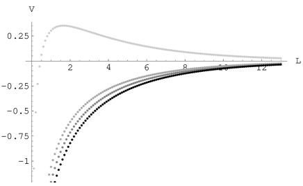
Figure 3: The static potential $V(L)$ for $QED_{3}$ (irreducible) with different values of the static charges magnetic moment $\mu=-2,0,2,20$ respectively from the darkest to the lightest curve. All curves were obtained for $m=0.1\,,\,c_{1}=1$ and vanishing non-minimal coupling $c_{2}=0$.

In figure 4 we take $\mu=0$ and analyze the effect of the magnetic moment of dynamical fermions ( Pauli term ) at fixed QED coupling $c_{1}=1$.

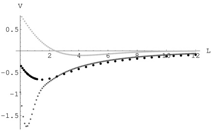
Figure 4: The static potential $V(L)$ for $QED_{3}$ (irreducible) with $\mu=0$ and different non-minimal couplings $c2=0.5,0.2,-0.5$ respectively from the darkest to the lightest curve. All curves were obtained for $m=0.1\,,\,c1=1$.

Similarly to the reducible case, the Pauli term leads also to a new, if compared to pure QED, repulsive force which is placed at small values of $L$. That happens even for tiny values of the Pauli coupling $c_{2}$. We have also let the couplings $\mu$ and $c_{2}$ appear altogether, the final output is shown in figure 5.

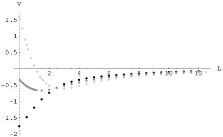
Figure 5: The static potential $V(L)$ for $QED_{3}$ (irreducible) with $\mu=3,0,-4$ respectively from the darkest to the lightest curve and $(c_{1},c_{2},m)=(1,0.5,0.1)$.

It is possible to turn the repulsive force which appears for a fixed value of $c_{2}$ into an attractive one by changing the static charges parameter $\mu$. Due to a term that depends on the product $\mu\,c_{2}$ , see (36), now the influence of $\mu$ is opposite to the pure QED ($c_{2}=0$) case. As we increase $\mu$ the repulsive force diminishes. In the specific case of fig.3, i.e., $(c_{1},c_{2},m)=(1,0.5,0.1)$ we checked that no repulsive force appears for $\mu\geq 1.67$.

3.3 Large mass limit

If we repeat the procedure of last section and send $m\to\infty$ while keeping $c_{1}$ and $c_{2}$ constant, the effective action (29) blows up at leading order. So we found more useful instead to take $m\to\infty$ and keep $e$ and $\gamma$ fixed in order to have a local theory, which becomes :

$${\cal L}_{eff}\, = \,-\left(1+\frac{e\gamma}{\pi}\right)\frac{1}{4}{F_{\mu\nu}F^{\mu\nu}}-\frac{1}{8\pi}\epsilon_{\mu\nu\alpha}A^{\mu}(e^{2}-4\gamma^{2}\Box)\partial^{\nu}A^{\alpha}+\frac{\zeta(\partial_{\mu}A^{\mu})^{2}}{2}$$ (37)

$$+ (A_{\nu}+\mu F_{\nu})\,j_{\rm ext}^{\nu}+{\cal O}\left(\frac{1}{m}\right)$$

Besides the well known generation of a Chern-Simons term, we also have a charge renormalization :

$$Q_{\rm ren}\,=\,\frac{Q}{\left(1+\frac{e\gamma}{\pi}\right)^{1/2}}\quad,$$ (38)

which is due to a cooperative effect with the Pauli interaction which in its turn also generates a higher order Chern-Simons term. This higher derivative term leads in general to an extra pole in the photon propagator. Both poles are real for $c2\geq-1/8\,(e\gamma/\pi\geq-1/2)$. The formula (20) becomes in this case:

$$V_{m\to\infty}(L)\,=\,-\frac{Q^{2}}{2\pi}\left(\frac{\pi(\pi+e\gamma)}{\gamma^{4}}\right)\int_{0}^{\infty}\frac{dk\,k\,J_{0}(kL)}{(k^{2}+m_{+}^{2})(k^{2}+m_{-}^{2})}$$ (39)

Where

$$m_{\pm}\,=\,\frac{\pi}{2\gamma^{2}}\left(1+\frac{e\gamma}{\pi}\pm\sqrt{1+\frac{2e\gamma}{\pi}}\right)$$ (40)

We can check that as $\gamma\to 0$ , which is the case of pure $QED_{3}$, $\gamma^{4}(k^{2}+m_{+}^{2})\to\pi^{2}$ while $m_{-}\to e^{2}/4\pi$. Thus, we are left with the well known massive photon of the Maxwell-Chern-Simons theory which is the effective action for pure $QED_{3}$ (irreducible) at $m\to\infty$. The simplicity of the photon propagator allows us to calculate $V(L)$ analytically. We just need the identity $1/(k^{2}+m_{-}^{2})-1/(k^{2}+m_{+}^{2})=(m_{+}^{2}-m_{-}^{2})/[(k^{2}+m_{+}^{2})(k^{2}+m_{-}^{2})]$. Consequently,

$$V_{m\to\infty}(L)\,=\,\frac{Q^{2}}{2\pi}\frac{1}{\sqrt{1+\frac{2e\gamma}{\pi}}}\left[K_{0}(m_{+}L)-K_{0}(m_{-}L)\right]$$ (41)

For $\gamma\to 0$ we reproduce, at leading order in $1/m$, the result of pure $QED_{3}$ obtained in [12]. Due to the relative sign among the modified Bessel functions the potential due to two different poles is now bounded for $L\to 0$, since $K_{0}(x\to 0)\to-\ln(x)$, and (41) becomes constant as $L\to 0$ (figure 7). Thus, the attractive force vanishes as $L\to 0$. For finite fermion mass the vanishing force can turn into a repulsive one. In figure 6 we compare the potential $V_{m\to\infty}$ with the numerical results obtained for $m=0.1,1$ in units such that $e^{2}/(16\pi)=0.1$ and $e\gamma/\pi=0.5$.

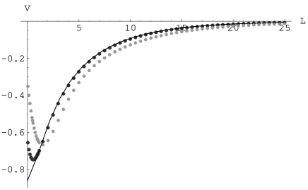
Figure 6: The static potential $V(L)$ for $QED_{3}$ (irreducible) for $m\to\infty$ (solid line), $m=1$ (dark dotts) and $m=0.1$ (light dotts) with couplings $mc_{1}=e^{2}/(16\pi)=0.1$ and $c_{2}=e\gamma/\pi=0.5$.

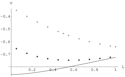
Figure 7: Blowing up the small $L$ region of figure 6.

The agreement, for most of the values of $L$, of the analytic formula (41) obtained at leading $1/m$ approximation with the numerical results already at $m=1$ is impressive. Of course, we have checked that larger values $m>1$ lead to an even better agreement. The repulsive force close to the origin only appears in the presence of a non-minimal coupling $\gamma\neq 0$ ( or $\mu\neq 0$ ) and a finite fermion mass.

4 Conclusion

In this work we have calculated, at leading order in $1/N$, the influence of a non-minimal coupling term on the static potential of QED with four and two components fermions. In the four components case the only effect of the vacuum polarization at large inter-charge separations is a screening of the original static charges. The potential keeps its classical shape $V(L)=-(Q_{\rm ren}^{2}/2\pi)\ln L$ at $L\to\infty$. Although parity is broken due to the non-minimal coupling the potential is still of confining type. The interesting point is that the generated Chern-Simons term is of higher order in the momentum and becomes negligible when compared with the Maxwell term as $k\to 0$. Consequently, the photon does not acquire mass which leads to a long range confining potential. Technically, the massless pole changes the factor $kJ_{0}(kL)$ in the integral for the potential $V(L)$ into $J_{0}(kL)/k$. Since the Bessel function is an oscillating function with decreasing amplitude, as $L\to\infty$ the integral is dominated by the region around $k=0$. In summary, the extra non-minimal couplings play no role in $V(L)$ for large distances as far as our $1/N$ approximation is valid.

In the irreducible case of pure QED it is well known that a traditional (linear in momentum) Chern-Simons term is generated and the classical pole at $k=0$ is replaced by a massive pole. This picture remains correct whatever values we choose for the new couplings $\gamma$ and $\mu$. Therefore we expect a short range screening potential as in pure irreducible QED. Indeed, we have obtained numerically $V(L\to\infty)\to 0$ as one can check in our figures of last section. Due to the lack of the pole at $k=0$ one can take the limit $L\to\infty$ before the integral in (24) is performed and the result will vanish as a consequence of $J_{0}(x\to\infty)\to 0$.

Concerning the presence of massive poles we have found basically three different regions in the coupling space. For strong enough Pauli coupling, when compared to the QED coupling ($c_{2}>c_{1}+\sqrt{c_{1}}$), we have a second massive pole besides the one generated by the usual Chern-Simons term. Our local limit $m\to\infty$ indicates that it is due to a higher order Chern-Simons term. If we decrease the Pauli coupling we reach an intermediate region and return to just one pole region as in pure QED. The most embarrassing result appears for very weak Pauli coupling ( or very strong QED coupling ), namely, we may have no poles at all. That happens, for instance, if $c_{2}<c_{1}-\sqrt{c_{1}}$ and $c_{1}>1$. In particular, it occurs in pure multiflavor QED ($c_{2}=0$) if $c_{1}=e^{2}/(16\pi m)>1$. Recalling that our effective action for the photon becomes exact for $N\to\infty$ the no pole region might indicate a breakdown of the $1/N$ expansion in the specific region $c_{2}<c_{1}-\sqrt{c_{1}}$ and ($c_{1}>1$).

Although at large distances the new couplings $\gamma$ and $\mu$ have not led us to new physical effects, at small distances we found a repulsive force of finite range between charges of opposite signs. This effect only appears for a finite fermion mass. As we increase the mass of the fermion the potential bents down and the repulsive effect disappears in agreement with our effective action (37) at $m\to\infty$. We do not have any explanation for the repulsive effect but we intent to return to that question by studying the existence of bound states in the future. We should remark that a repulsive effect between charges of opposite signs, similar to a centrifugal barrier, was observed before in [17] in irreducible $QED_{3}$ with a Thirring term with positive coefficient (opposite sign to the one used in [16]). However, we stress that our numerical calculations were obtained without any approximation for large masses or small couplings as in [17]. The similarity between the addition of the Thirring term and the non-minimal coupling might have its root in the fact that both the Thirring and the non-minimal coupling constants $\gamma$ used here have the same mass dimensionality $m^{-1/2}$. Studies of duality in vector models in $D=2+1$ coupled to fermionic matter [25, 26, 27] indicate that there might be a more direct relation between the Pauli and the Thirring term in $d=2+1$ dimensions.

Finally, we point out that another motivation to study the effect of a non-minimal coupling of the Pauli-type is the fact that this term is radioactively generated anyway (irreducible case), at least in a Maxwell Chern-Simons theory [28, 29]. Furthermore, it has been recently shown in [29] that if the Chern-Simons term is not present from the start the Pauli term will be generated with an infinite coefficient which points to the need of having this term from the beginning in order to have an infrared finite theory. In our calculations we suppressed a possible Chern-Simons term in the starting Lagrangian because we would like to single out the effect of the Pauli-type term. It is clearly desirable to have both terms from the start but the profusion of coupling constants make the analysis made here much more involved which is out of the scope of this work.

5 Acknowledgments

This work was partially supported by CNPq, FAPESP and CAPES-PROAP, Brazilian research agencies. Discussions with Antonio S. de Castro, Alvaro de Souza Dutra and Marcelo Hott are acknowledged. We also thank M. H. for bringing references [5, 20] to our attention.

References

- [1] N. Seiberg and E. Witten, Nucl. Phys. B426 (1994) 19.
- [2] H. J. Rothe, K. D. Rothe and J. A. Swieca, Phys. Rev. D 19 (1979) 3020.
- [3] D. J. Gross, I. R. Klebanov, A. V. Matytsin and A. V. Smilga, Nucl. Phys. B 461 (1996) 109.
- [4] E. Abdalla, R. Mohayee and A. Zadra, Int. J. Mod. Phys. A 12 (1997) 4539.
- [5] P. Maris, Phys. Rev. D 52(1995) 6087.
- [6] C.P. Burgess and F. Quevedo, Nucl. Phys. B421 (1994) 373, C.P. Burgess, C. Lutken and F. Quevedo, Phys. Lett. B336 (1994) 1894.
- [7] E. Fradkin and F. A. Schaposnik, Phys. Lett. B 338 (1994) 253. G. Rossini and F. A. Schaposnik, Phys. Lett. B 338 (1994) 465.
- [8] D. G. Barci, C.D. Fosco and L. E. Oxman, Phys. Lett. B 375 (1996) 367.
- [9] R. Banerjee, Nucl. Phys. 465 (1996) 157.
- [10] R. Banerjee and E. C. Marino, Phys. Rev. D 56 (1997) 3763.
- [11] D. Dalmazi, A. de Souza Dutra and M. Hott, Phys. Rev. D 67 (2003) 125012.
- [12] E. Abdalla and R. Banerjee, Phys. Rev. Lett (1998) 238.
- [13] E. Abdalla, R. Mohayee and A. Zadra, Int. J. Mod. Phys. A 12 (1997) 4539.
- [14] D. Dalmazi, A. de Souza Dutra and M. Hott, Phys. Rev. D 61 (2000) 125018.
- [15] S. Deser, R. Jackiw and S. Templeton, Annals of Phys. 140 (1982) 372.
- [16] E. M. C. Abreu, D. Dalmazi, A. de Souza Dutra and M. Hott, Phys.Rev. D65 (2002) 125030.
- [17] S. Ghosh, Journal of Physics A 33 (2000) 1915, ibidem page 4213.
- [18] P. Gaete, Phys.Rev. D64 (2001) 027702.
- [19] J. Stern, Phys. Lett. B265 (1991) 119.
- [20] Y. Georgelin and J.C. Wallet, Mod. Phys. Letters A7 (1992) 1149.
- [21] M. E. Carrington and G. Kunstatter, Phys.Rev. D51 (1995) 1903.
- [22] F.A.S. Nobre and C.A.S. Almeida, Phys.Lett.B455 (1999) 213.
- [23] C. R. Hagen, Phys.Lett. B470 (1999) 119.
- [24] N. Itzhaki, Phys.Rev. D67 (2003) 65008.
- [25] M. Gomes, L. C. Malacarne and A. J. da Silva, Phys. Lett. B439 (1998) 137.
- [26] M.A. Anacleto, A. Ilha, J.R.S. Nascimento, R.F. Ribeiro and C. Wotzasek, Phys. Lett. B504 (2001) 268.
- [27] D. Dalmazi, Journal of Physics A37 (2004) 2487.
- [28] I.I. Kogan and G.W. Semenoff, Nucl. Phys. B368 (1991) 718.
- [29] A. Das and S. Perez, Phys. Lett. B581 (2004) 182.
- [30] C. J. Burden, J. Praschifka and C. D. Roberts Phys.Rev. D46 (1992) 2695.