1 Introduction

In constructing unified theories with extra dimensions [1]–[3], it is crucial to obtain topological defects and localization of massless or nearly massless modes on the defect. Walls in five-dimensional theories are the simplest of the topological defects leading to the four-dimensional world-volume. In constructing topological defects, supersymmetric (SUSY) theories are helpful, since partial preservation of SUSY automatically gives a solution of equations of motion [4]. These states are called BPS states. The simplest of these BPS states is the wall [5, 6]. The resulting theory tend to produce an ${\cal N}=1$ SUSY theory on the world volume, which can provide realistic unified models with the desirable properties [7]. Although scalars and spinors can be obtained as localized modes on the wall [8], it has been difficult to obtain localized massless gauge bosons in five dimensions, in spite of many interesting proposals, especially in lower dimensions [9]–[16]. Recently a model of the localized massless gauge bosons on the wall has been obtained for Abelian gauge theories using SUSY QED interacting with tensor multiplets [14, 15]. Walls in non-Abelian gauge theories are called non-Abelian walls. They are expected to help obtaining non-Abelian gauge bosons localized on the world volume. Moreover, non-Abelian wall solutions have rich structures and are interesting in its own right. BPS walls in a non-Abelian SUSY gauge theories have recently been studied in lower dimensions in a particular context [16].

The purpose of this paper is to construct BPS walls in five-dimensional non-Abelian gauge theories with eight supercharges and to obtain the effective theories of moduli on the four-dimensional world-volume. In particular we study the $U(N_{\rm C})$ gauge theory with $N_{\rm F}(>N_{\rm C})$ flavors of hypermultiplets in the fundamental representation. To obtain discrete vacua, we consider non-degenerate masses for hypermultiplets, and the Fayet-Iliopoulos (FI) parameter is introduced [17]. By taking the limit of infinite gauge coupling, we obtain exact BPS multi-wall solutions with generic moduli parameters covering the complete moduli space. For a restricted class of moduli parameters called $U(1)$-factorizable moduli, we also obtain exact BPS multi-wall solutions for certain values of finite gauge coupling. We find that the total moduli space is a compact complex manifold, the Grassmann manifold $G_{N_{\rm F},N_{\rm C}}\equiv{SU(N_{\rm F})\over SU(N_{\rm C})\times SU(N_{\rm F}-N_{\rm C})\times U(1)}$ as reported in [18]. Each moduli parameter provides a massless field for the effective field theory on the world volume of walls. We find explicitly Nambu-Goldstone scalars associated with the spontaneously broken global symmetry. We also identify those massless scalars that are not explained by the spontaneously broken symmetry and are called quasi-Nambu-Goldstone scalars. We find it convenient to introduce a matrix function $S(y)$ as a function of the extra-dimensional coordinate and constant moduli matrices $H_{0}^{i}$ to describe the solution. The redundancy of the description is expressed as a global symmetry $GL(N_{\rm C},{\bf C})$ of these data $(S,H_{0}^{i})$. This symmetry turns out to be very useful and eventually be promoted to a local gauge symmetry when we consider effective theories on the world volume of walls. Therefore we call the symmetry the world-volume symmetry. We also obtain a general formula for the metric in moduli space which gives the effective theory of moduli fields on the world volume. The formula can be reduced to an explicit integral representation in the case of infinite gauge coupling. We also establish a duality between BPS wall solutions with $U(N_{\rm C})$ color and $N_{\rm F}$ flavor and those with $U(\tilde{N}_{\rm C}\equiv N_{\rm F}-N_{\rm C})$ color and $N_{\rm F}$ flavor.

Our solutions and their moduli space are unchanged under dimensional reduction to two, three and four space-time dimensions. In particular, in four space-time dimensions, there exists a long history for construction of BPS solitons and their moduli space in the gauge-Higgs system. A beautiful method for construction of instantons was given by Atiyah, Hitchin, Drinfeld and Manin (ADHM) [22]. It was modified by Nahm to the one for BPS monopoles [23]. Recently the moduli space for non-Abelian vortices has been constructed by Hanany and Tong [21]. However, a systematic method for construction of walls in non-Abelian gauge theories has not been obtained although there exist some for walls in Abelian gauge theories and/or nonlinear sigma models derivable from Abelian gauge theories [24, 25, 26, 27, 14]. Our method presents the last gap for the construction of solitons and moduli space in the gauge-Higgs system. Our wall moduli space as well as the moduli space of vortices are constructed by the Kähler quotient while moduli spaces of instantons and monopoles are constructed by the hyper-Kähler quotient. One interesting feature for non-Abelian walls may be that the total moduli space is finite dimensional in contrast to total moduli spaces for other solitons which are infinite dimensional.

Since we are interested in wall solutions with Poincaré invariance in the wall world-volume, only the extra-dimensional component $W_{y}$ may be nontrivial for the gauge field. One can always choose a gauge of the original local gauge symmetry to eliminate the extra-dimensional component $W_{y}$ of gauge field in the case of $U(1)$ gauge theories. Therefore all the explicit wall solutions so far obtained have vanishing gauge field configurations [25, 12, 14]. In the case of the non-Abelian gauge group, it is usually convenient to eliminate all the vector multiplet scalars for generators outside of the Cartan subalgebra ${\cal H}$, and all the gauge fields for generators in the Cartan subalgebra: $\Sigma^{I\not\in{\cal H}}=0$, $W_{y}^{I\in{\cal H}}=0$. We find that our BPS multi-wall solutions for generic moduli have nontrivial gauge field configurations: $W_{y}^{I\not\in{\cal H}}\not=0$. We will also give a gauge invariant description of these nontrivial vector multiplet configurations and evaluate these gauge invariant quantities for explicit examples.

The SUSY vacua in our $U(N_{\rm C})$ model are found to be the color-flavor locking form specified by the non-vanishing flavor $A_{r}$ for each color component $r$, such as $\langle A_{1}\cdots A_{N_{\rm C}}\rangle$ abbreviated as $\langle A\rangle$. BPS multi-wall solutions interpolate between two SUSY vacua which are specified by boundary conditions: a SUSY vacuum $\langle A_{1}\cdots A_{N_{\rm C}}\rangle$ at $y=\infty$ and another SUSY vacuum $\langle B_{1}\cdots B_{N_{\rm C}}\rangle$ at $y=-\infty$. The boundary condition at $\pm\infty$ defines a topological sector denoted as $\langle A_{1}\cdots A_{N_{\rm C}}\rangle\leftarrow\langle B_{1}\cdots B_{N_{\rm C}}\rangle$. The total moduli space is defined by a sum over $k$ of the moduli spaces of $k$-walls ${\cal M}^{k}_{N_{\rm F},N_{\rm C}}$, but may also be expressed as a sum over the topological sectors ${\cal M}^{\langle A\rangle\leftarrow\langle B\rangle}_{N_{\rm F},N_{\rm C}}$ defined by boundary conditions at $y=\pm\infty$:

$$G_{N_{\rm F},N_{\rm C}}=\sum_{k}{\cal M}^{k}_{N_{\rm F},N_{\rm C}}=\sum_{\langle A\rangle\leftarrow\langle B\rangle}{\cal M}^{\langle A\rangle\leftarrow\langle B\rangle}_{N_{\rm F},N_{\rm C}}.$$ (1.1)

Among various BPS walls, there are walls interpolating between two vacua with identical labels except one label that have adjacent flavors: $\langle A_{1}\cdots A_{N_{\rm C}}\rangle\leftarrow\langle B_{1}\cdots B_{N_{\rm C}}\rangle$ with $A_{j}=B_{j},\,j\not=i$, and $A_{i}+1=B_{i}$. These walls are building blocks of multi-walls and are called elementary walls. We find that a quantum number $(A_{i},A_{i}+1)$ can be ascribed to the elementary wall with $A_{i}+1=B_{i}$ and a matrix algebra can be formulated to describe the non-Abelian walls. Composite walls made of several elementary walls can be represented by a product of matrices corresponding to constituent elementary walls. If the matrices do not commute, the commutator gives a single wall made by compressing the two walls. We call such a wall compressed wall. This is the situation for Abelian walls. On the other hand, we can also have commuting matrices for non-Abelian walls. If the matrices are commuting, the two elementary walls are called penetrable, since the intermediate vacuum changes character while the constituent walls go through each other maintaining their identities by changing from one sign of the relative position to the other sign.

In Sec. 2, we introduce our model, work out SUSY vacua with a convenient diagrammatic representation, and obtain $1/2$ BPS equations. In Sec. 3, exact solutions of the BPS equations are obtained both for infinite and for finite gauge couplings, by introducing moduli matrices and the world-volume symmetry. In Sec. 4, explicit solutions at infinite coupling are presented for a number of illustrative examples. In Sec. 5, the topology and metric of the moduli space of the non-Abelian BPS wall solutions are studied. In Sec. 6, we discuss the implications of our results and future directions of research. A number of useful details are described in several Appendices.

2 The Model, SUSY Vacua and BPS Equations

2.1 The Model

Since we are interested in theories in five dimensions, we need eight supercharges. With this minimum number of supersymmetry (SUSY), simple building blocks are vector multiplets and hypermultiplets. Wall solutions require discrete vacua, which can be obtained by considering $U(1)$ factors besides semi-simple gauge group [17]. We denote the gauge group suffix and flavor group suffix in our fundamental theory by the uppercase letters G and F, respectively. The $U(1)_{\rm G}$ vector multiplet with coupling constant $g_{0}$ consists of a $U(1)_{\rm G}$ gauge field $W_{M}^{0}$, a real scalar field $\Sigma^{0}$, a $SU(2)_{R}$ triplet of real auxiliary field $Y^{a0}$, and an $SU(2)_{R}$ doublet of gauginos $\lambda^{i0}$. We denote space-time indices by $M,N,\cdots=0,1,2,3,4$, and $SU(2)_{R}$ triplet, doublet indices by $a,i$ respectively. The $U(1)_{\rm G}$ part of vector multiplets allows us to introduce the FI term which gives rise to discrete vacua once mass terms for hypermultiplets are introduced [17].

We also have a non-Abelian vector multiplet for a semi-simple gauge group $G$ with coupling constant $g$. It consists of a gauge field $W_{M}$, a scalar $\Sigma$, auxiliary fields $Y^{a}$, and gauginos $\lambda^{i}$, which are now in the adjoint representation of $G$. We use a matrix notation for these component fields, such as $\Sigma=\Sigma^{I}T_{I}$. We denote the Hermitian generators in the Lie algebra ${\cal G}$ of the gauge group $G$ as $T^{I}\in{\cal G}\ (I=1,2,\cdots,{\rm dim}(G))$, which satisfy the following normalization condition and commutation relation

$${\rm Tr}(T_{I}T_{J})=T({\cal R})\delta_{IJ},\ \ \ [T_{I},T_{J}]=if_{IJ}{}^{K}T_{K},$$ (2.1)

where $f_{IJ}{}^{K}$ are the structure constants of the gauge group $G$, and $T({\cal R})$ is the normalization constant for the representation ${\cal R}$. Furthermore, we denote the generators in the Cartan subalgebra ${\cal H}$ of ${\cal G}$ by a suffix $x$ as $T^{x}\in{\cal H}$. For later convenience, we denote the generator of the $U(1)$ factor group as $T^{0}$ with the same normalization as the non-Abelian group generators (2.1). Moreover, we collectively denote generators as $T^{I}$ with $I$ running over $I=0$ for the $U(1)$ and $I=1,\cdots,{\rm dim}({\cal G})$ for the non-Abelian group. We also denote gauge couplings as $g_{I}$ ($I=0,1,\cdots,{\rm dim}({\cal G})$), with $g_{I}\equiv g$ for $I=1,\cdots,{\rm dim}({\cal G})$. Similarly we also combine the $U(1)$ generator with those in the Cartan subalgebra to denote diagonal generators: $T^{x}$ with $x=0,1,\cdots,{\rm dim}({\cal H})$.

We have hypermultiplets as matter fields, consisting of $SU(2)_{R}$ doublet of complex scalar quark fields $H^{irA}$, $SU(2)_{R}$ doublet of auxiliary fields $F_{i}^{rA}$, and Dirac fields $\psi^{rA}$. Color indices $r,s,\cdots$ run over $1,2,\cdots,{\cal R}$ where ${\cal R}$ denotes the dimension of the representation of the hypermultiplet, whereas $A,B,\cdots=1,2,\cdots,N_{\rm F}$ stand for flavor indices. We consider $N_{\rm F}>N_{\rm C}$ to obtain disconnected SUSY vacua appropriate for constructing walls.

We shall consider a model with minimal kinetic terms for vector and hypermultiplets. The eight supercharges allow only a few parameters in our model: gauge coupling constants $g_{0}$ for $U(1)_{\rm G}$, and $g$ for the non-Abelian semi-simple gauge group $G$, the masses of $A$-th hypermultiplet $m_{A}$, and the FI parameters $\zeta^{a}$ for the $U(1)_{\rm G}$ vector multiplet. Then the bosonic part of our Lagrangian reads

$$\mathcal{L}_{\rm bosonic} \!\!\!= \!\!\!-\sum_{I\geq 0}\frac{1}{4g_{I}^{2}}F_{MN}^{I}(W)F^{IMN}(W)$$ (2.2)

$$\!\!\!+\sum_{I\geq 0}\frac{1}{2g_{I}^{2}}\mathcal{D}_{M}\Sigma^{I}\mathcal{D}^{M}\Sigma^{I}$$

$$\!\!\!{}-\zeta^{a}Y^{a0}+\sum_{I\geq 0}\frac{1}{2g_{I}^{2}}(Y^{aI})^{2}$$

$$\!\!\!{}+(\mathcal{D}_{M}H^{irA})^{*}\mathcal{D}^{M}H^{irA}-(H^{irA})^{*}[(\Sigma-m_{A})^{2}]^{r}{}_{s}H^{isA}$$

$$\!\!\!{}+(H^{irA})^{*}(\sigma^{a})^{i}{}_{j}(Y^{a})^{r}{}_{s}H^{jsA}+(F_{i}^{rA})^{*}F_{i}^{rA},$$

where the summation over group indices $I$ is explicitly denoted. In the following, however, we will suppress the summation with the understanding that the sum over repeated indices $I$ should be done including $I=0$, unless stated otherwise. Summation over repeated indices is also implied for other indices. The covariant derivatives are defined as $\mathcal{D}_{M}H^{irA}=(\partial_{M}\delta_{s}^{r}+i(W_{M}^{I})^{r}{}_{s})H^{isA}\ (I=0,1,\cdots,{\rm dim}(G))$, $\mathcal{D}_{M}\Sigma=\partial_{M}\Sigma+i[W_{M},\Sigma]$, and field strength is defined as $F_{MN}=\frac{1}{i}[\mathcal{D}_{M},\mathcal{D}_{N}]=\partial_{M}W_{N}-\partial_{N}W_{M}+i[W_{M},W_{N}]$ and our convention of metric is $\eta_{MN}={\rm diag}(+1,-1,-1,-1,-1)$.

In this paper, we assume non-degenerate mass parameters $m_{A}$ unless stated otherwise. Then the flavor symmetry reduces to

$$G_{\rm F}=U(1)_{\rm F}^{N_{\rm F}-1},$$ (2.3)

where $U(1)_{\rm F}$ corresponding to common phase is gauged by $U(1)_{\rm G}$ local gauge symmetry. We choose the order of the mass parameters as $m_{A}>m_{A+1}$ for all $A$.

2.2 SUSY Vacua and its Diagrammatic Representation

SUSY vacua can be obtained by requiring vanishing vacuum energy. Let us first write down equations of motion for auxiliary fields

$$Y^{a0} \!\!\!= \!\!g_{0}^{2}[\zeta^{a}-(H^{irA})^{*}(\sigma^{a})^{i}{}_{j}(T_{0})^{r}{}_{s}H^{jsA}],$$ (2.4)

$$Y^{aI} \!\!\!= \!\!\!-g^{2}(H^{irA})^{*}(\sigma^{a})^{i}{}_{j}(T_{I})^{r}{}_{s}H^{jsA},\ \ (I\not=0),$$ (2.5)

$$F_{i}^{rA} \!\!\!= \!\!\!0.$$ (2.6)

After eliminating auxiliary fields, we obtain the on-shell version of the bosonic part of the Lagrangian

$$\mathcal{L}_{\rm bosonic} \!\!\!= \!\!\!-\frac{1}{4g_{I}^{2}}F_{MN}^{I}(W)F^{IMN}(W){}+\frac{1}{2g_{I}^{2}}\mathcal{D}_{M}\Sigma^{I}\mathcal{D}^{M}\Sigma^{I}$$ (2.7)

$$\!\!\!{}+(\mathcal{D}_{M}H^{irA})^{*}\mathcal{D}^{M}H^{irA}-V,$$

where the scalar potential $V$ is given by

$$V \!\!\!= \!\!\!\frac{1}{2g_{I}^{2}}(Y^{aI})^{2}+(F_{i}^{rA})^{*}F_{i}^{rA}+(H^{irA})^{*}[(\Sigma-m_{A})^{2}]^{r}{}_{s}H^{isA}$$ (2.8)

$$\!\!\!= \!\!\!\frac{g_{I}^{2}}{2}[\zeta^{a}\delta_{0I}-(H^{irA})^{*}(\sigma^{a})^{i}{}_{j}(T^{I})^{r}{}_{s}H^{jsA}]^{2}$$

$$\!\!\!\hskip 56.9055pt{}+(H^{irA})^{*}[(\Sigma-m_{A})^{2}]^{r}{}_{s}H^{isA}.$$

The vanishing vacuum energy requires both contributions from vector and hypermultiplets to vanish. Conditions of vanishing contribution from vector multiplet can be summarized to one equation as

$$(H^{irA})^{*}(\sigma^{a})^{i}{}_{j}(T_{I})^{r}{}_{s}H^{jrA}=\zeta^{a}\delta_{0I},\ (I=0,1,\cdots,{\rm dim}(G)).\quad$$ (2.9)

The $SU(2)_{R}$ symmetry allows us to choose the FI parameters to lie in the third direction without loss of generality

$$\zeta^{a}=(0,\ 0,\ \zeta),\ \ \ \zeta>0.$$ (2.10)

Then the SUSY condition (2.9) for the vector multiplets is reduced to

$$a=3: \!\!\ (H^{1rA})^{*}(T_{I})^{r}{}_{s}H^{1sA}-(H^{2rA})^{*}(T_{I})^{r}{}_{s}H^{2sA}=\zeta\delta_{0I},\qquad$$ (2.11)

$$a=1,2: \!\!\ (H^{1rA})^{*}(T_{I})^{r}{}_{s}H^{2sA}=0,$$ (2.12)

where $r,s=1,2,\cdots,{\cal R}$, $A=1,2,\cdots,N_{\rm F}$ and $I=0,1,2,\cdots,{\rm dim}(G)$. Requiring the vanishing contribution to vacuum energy from hypermultiplets gives the SUSY condition for hypermultiplets as

$$(\Sigma^{0}T_{0}+\sum_{I\geq 1}^{{\rm dim}(G)}\Sigma^{I}T_{I}-m_{A}\mathbf{1}_{{\cal R}})^{r}{}_{s}H^{isA}=0,\$$ (2.13)

for each index $A$. By local gauge transformations of $G$, we can always choose $\Sigma^{I\not\in{\cal H}}=0$. To parametrize the remaining vector multiplet scalars belonging to the Cartan subalgebra ${\cal H}$, we introduce orthogonal matrices $T_{x}$ as

$$(T_{x})^{r}{}_{s} \equiv \delta^{r}{}_{s}n_{xr}({\cal R}),\quad{\rm for~{}}x=0,1,2,\dots,{\rm dim}({\cal H}),\qquad$$ (2.14)

where $n_{xr}$ is the $U(1)_{x}$-charge of the scalar carrying the color index $r$, and note that $n_{xr}$ have the following properties due to the traceless condition of $T_{x}$ and the normalization (2.1)

$$n_{0r}({\cal R})=\sqrt{T(\cal R)\over\cal R},\quad\sum_{r=1}^{\cal R}n_{x(\not=0)r}({\cal R})=0,\quad$$

$$\sum_{r=1}^{\cal R}n_{xr}({\cal R})n_{yr}({\cal R})=T({\cal R})\,\delta_{xy}.$$ (2.15)

Rewriting the condition (2.13) with $n_{xr}({\cal R})$, we obtain

$$\left\{\left({\Sigma^{0}\over\sqrt{2\cal R}}-m_{A}\right)+\sum_{x=1}^{{\rm dim}({\cal H})}\Sigma^{x}n_{xr}({\cal R})\right\}H^{irA}$$

$$=\left\{\sum_{x=0}^{{\rm dim}({\cal H})}\Sigma^{x}n_{xr}({\cal R})-m_{A}\right\}H^{irA}=0$$ (2.16)

for each index $A$. In order to have a non-vanishing hypermultiplet scalar $H^{irA}$ with the color $r$ and the flavor $A$, we need to require the corresponding coefficient in Eq. (2.16) to vanish:

$$(\Sigma)^{r}{}_{r}=\sum_{x=0}^{{\rm dim}({\cal H})}\Sigma^{x}n_{xr}({\cal R})=m_{A}.$$ (2.17)

Let us consider a $({\rm dim}({\cal H})+1)$-dimensional space $\vec{\Sigma}\equiv(\Sigma^{0},\Sigma^{x=1},\cdots,\Sigma^{x={\rm dim}({\cal H})})$ of the vector multiplet scalars. The condition (2.17) implies that the region in $\vec{\Sigma}$ for a non-vanishing hypermultiplet scalar $H^{irA}$ should be contained in a ${\rm dim}({\cal H})$-dimensional hyperplane, which contains a point $\vec{\Sigma}=(\sqrt{2\cal R}m_{A},0,\cdots,0)$ and is orthogonal to the vector $\vec{n}_{r}({\cal R})$ with component $(\vec{n}_{r})_{x}\equiv n_{xr}$. Obviously, two scalars $H^{irA}$ and $H^{irB}$ with the same color index $r$ can be non-vanishing only if $m_{A}=m_{B}$. Vacua with the $n$ non-vanishing scalars should lie in the $({\rm dim}({\cal H})+1-n)$-dimensional hyperplane in $\vec{\Sigma}$. These hyperplanes can easily be visualized diagrammatically in $\vec{\Sigma}$ space. These diagrams are quite useful to understand the structure of the vacua intuitively, and to construct the domain walls interpolating between these vacua as we see below.

We shall discuss mainly the cases where there are non-vanishing scalars carrying flavor $A_{r}$ for the $r$-th color component, ($H^{irA_{r}}\not=0$). In these cases, Eqs. (2.17) and (2.15) determine the scalar $\Sigma^{x}$ in terms of $n_{xr}(\cal R)$ as

$$\Sigma^{x}=\frac{1}{T({\cal R})}\sum_{r=1}^{\cal R}n_{xr}({\cal R})\,m_{A_{r}}.$$ (2.18)

In particular $\Sigma^{0}$ is given by an average value of the mass parameters,

$$\Sigma^{0}=\frac{1}{\sqrt{T({\cal R}){\cal R}}}\sum_{r=1}^{\cal R}\,m_{A_{r}},$$ (2.19)

which is independent of gauge-choices.

2.3 SUSY Vacua for $U(N_{\rm C})$ Gauge Group with $N_{\rm F}$ Flavors

The procedure to solve the SUSY conditions (2.11) and (2.12) for the vector multiplets depends on details of the system. In this paper, we mostly consider a simple example of the $U(1)\times G=U(N_{\rm C})$ gauge group, and $N_{\rm F}$ hypermultiplets in the fundamental representation of $U(N_{\rm C})$, for which we choose $T({\cal R})=1/2$. We assume non-degenerate mass parameters : with the ordering $m_{A}>m_{A+1}$ for all $A$ as was mentioned below Eq. (2.3).

It is convenient to combine the $N_{\rm F}$ hypermultiplets in the fundamental representation into the following $N_{\rm C}\times N_{\rm F}$ matrix

$$H^{i}\equiv\left(\begin{array}[]{cccc}H^{i11}&H^{i12}&\cdots&H^{i1N_{\rm F}}\\ H^{i21}&H^{i22}&\cdots&H^{i2N_{\rm F}}\\ \vdots&\vdots&\ddots&\vdots\\ H^{iN_{\rm C}1}&H^{iN_{\rm C}2}&\cdots&H^{iN_{\rm C}N_{\rm F}}\end{array}\right).$$ (2.24)

In the following, we will denote this matrix as $H^{i}$, while its $rA$ components are denoted as $H^{irA}$. We also use $N_{\rm F}\times N_{\rm C}$ matrix $H^{i}{}^{\dagger}$ whose components are $(H^{i}{}^{\dagger})_{Ar}\equiv(H^{irA})^{*}$. The SUSY condition (2.11) for vector multiplets can be rewritten in terms of this matrix as

$$H^{1}H^{1\dagger}-H^{2}H^{2\dagger}=2\zeta T_{0}=c\mathbf{1}_{N_{\rm C}},$$ (2.25)

where we rescaled the FI parameter $\zeta$ to define $c$

$$c\equiv\zeta\sqrt{2/N_{\rm C}}.$$ (2.26)

Another SUSY condition for vector multiplets, (2.12) becomes

$$H^{2}H^{1\dagger}=0.$$ (2.27)

Since we assume non-degenerate masses for hypermultiplets, we find from the conditions (2.16), (2.25) and (2.27) that only one flavor $A=A_{r}$ can be non-vanishing for each color component $r$ of hypermultiplet scalars $H^{irA}$ with

$$H^{1rA}=\sqrt{c}\,\delta^{A_{r}}{}_{A},\quad H^{2rA}=0,$$ (2.28)

since $c=\zeta\sqrt{2/N_{\rm C}}>0$ as defined in Eq. (2.10). Here we used global gauge transformations to eliminate possible phase factors. This is often called the color-flavor locking vacuum. The vector multiplet scalars $\Sigma^{x}$ is determined in $\vec{\Sigma}$ as intersection points of $N_{\rm C}$ hyperplanes defined by (2.17), as illustrated in Fig. 1

$${1\over\sqrt{2N_{\rm C}}}\Sigma^{0}+{1\over 2}\Sigma^{3}+{1\over\sqrt{3}}\Sigma^{8}+\cdots = m_{A_{1}},$$

$${1\over\sqrt{2N_{\rm C}}}\Sigma^{0}-{1\over 2}\Sigma^{3}+{1\over\sqrt{3}}\Sigma^{8}+\cdots = m_{A_{2}},$$

$${1\over\sqrt{2N_{\rm C}}}\Sigma^{0}\quad\qquad-{2\over\sqrt{3}}\Sigma^{8}+\cdots = m_{A_{3}},$$ (2.29)

$$\vdots$$ .

These discrete vacua are equivalently expressed in the matrix notation as

$$\Sigma={\rm diag.}(m_{A_{1}},\,m_{A_{2}},\,\cdots,\,m_{A_{N_{\rm C}}}).$$ (2.30)

We denote a SUSY vacuum specified by a set of non-vanishing hypermultiplet scalars with the flavor $\{A_{r}\}$ for each color component $r$ as

$$\langle A_{1}\,A_{2}\,\cdots\,A_{N_{\rm C}}\rangle.$$ (2.31)

Since global gauge transformations can exchange flavors $A_{r}$ and $A_{s}$ for the color component $r$ and $s$, respectively, the ordering of the flavors $A_{1},\cdots,A_{N_{\rm C}}$ does not matter in considering only vacua: $\langle 123\rangle=\langle 213\rangle$. Thus a number of SUSY vacua is given by [17]

$${}_{N_{\rm F}}C_{N_{\rm C}}={N_{\rm F}!\over N_{\rm C}!(N_{\rm F}-N_{\rm C})!}$$ (2.32)

and we usually take $A_{1}<A_{2}<\cdots<A_{N_{\rm C}}$.

Walls interpolate between two vacua at $y=\infty$ and $y=-\infty$. These boundary conditions at $y=\pm\infty$ define topological sectors, such as $\langle 12\rangle\leftarrow\langle 34\rangle$. (Multi-)walls are classified by the topological sectors. Clearly $\langle 12\rangle\leftarrow\langle 34\rangle$ is identical to $\langle 12\rangle\leftarrow\langle 43\rangle$.

When we consider walls, however, it is often convenient to fix a gauge in presenting solutions. The gauge transformations allow us to eliminate all the vector multiplet scalars $\Sigma^{I\not\in{\cal H}}$ for generators outside of the Cartan subalgebra ${\cal H}$, and all the gauge fields $W_{y}^{I\in{\cal H}}$ in the Cartan subalgebra ${\cal H}$. In this gauge, gauge fields $W_{y}^{I\not\in{\cal H}}$ can no longer be eliminated, since gauge is completely fixed. We shall usually use this gauge

$$\Sigma^{I\not\in{\cal H}}=0,\qquad W_{y}^{I\in{\cal H}}=0$$ (2.33)

in this paper unless otherwise stated. If we wish, we can choose another gauge where the extra dimension component $W_{y}^{I}$ of the gauge field vanishes for all the generators. Then all components of vector multiplet scalars $\Sigma^{I}$ including those out of Cartan subalgebra become nontrivial. In that gauge, our BPS multi-wall solutions are expressed by nontrivial vector multiplet scalars $\Sigma^{I}$ for all the generators, instead of gauge fields $W_{y}^{I}$.

When gauge is fixed in any one of these gauge choices, the ordering of flavors have physical significance, since changing one side of the boundary condition ($y=+\infty$) while keeping the other side ($y=-\infty$) requires local gauge transformations which will no longer be allowed. For example, we denote the wall connecting two vacua labeled by $\langle 12\rangle$ at $y=+\infty$ and $\langle 34\rangle$ at $y=-\infty$ as $\langle 12\leftarrow 34\rangle$ in the gauge fixed representation. The wall connecting vacua $\langle 12\rangle$ and $\langle 34\rangle$ is different from $\langle 12\rangle$ and $\langle 43\rangle$ in the gauge-fixed representation : $\langle 12\leftarrow 34\rangle\not=\langle 12\leftarrow 43\rangle$.

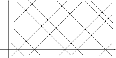
Figure 1: Diagrammatic representation of vacua for $N_{\rm C}=2$ case. Dashed lines are defined by $\Sigma^{0}+\Sigma^{3}=2m_{A}$ and $\Sigma^{0}-\Sigma^{3}=2m_{A}$. Vacua are given as intersection points of these lines except for $\Sigma^{3}=0$, because of Eq. (2.27).

2.4 Half BPS Equations for Domain Walls

We assume $g_{0}=g$ in the following. Let us obtain the BPS equations for domain walls interpolating between two SUSY vacua. The SUSY transformation laws of fermions of vector multiplets and hypermultiplets are given by

$$\delta_{\varepsilon}\lambda^{i} \!\!\!=\!\!\! \Bigl{\{}\frac{1}{2}\gamma^{MN}F_{MN}(W)+\gamma^{M}{\cal D}_{M}\Sigma\Bigl{\}}\varepsilon^{i}+i(Y^{a}\sigma^{a})^{i}{}_{j}\varepsilon^{j},\quad\ \$$ (2.34)

$$\delta_{\varepsilon}\psi \!\!\!=\!\!\! \sqrt{2}\Bigl{\{}-i\gamma^{M}{\cal D}_{M}H^{i}+\!\Sigma H^{i}-H^{i}M\Bigl{\}}\epsilon_{ij}\varepsilon^{j}+\!\sqrt{2}F_{i}\varepsilon^{i},\quad\ \$$ (2.35)

where we use $N_{\rm F}\times N_{\rm F}$ Hermitian mass matrix $M$ defined by

$$(M)^{A}{}_{B}\equiv m_{A}\delta^{A}{}_{B}.$$ (2.36)

To obtain wall solutions, we assume that all fields depend only on the coordinate of one extra dimension $x^{4}$ which we denote as $y$. We also assume the Poincaré invariance on the four-dimensional world volume of the wall, implying

$$F_{MN}(W)=0,\ \ W_{\mu}=0,$$ (2.37)

where we take $x^{\mu}=(x^{0},x^{1},x^{2},x^{3})$ as four-dimensional world-volume coordinates. Note that $W_{y}$ need not vanish. We demand that half of supercharges defined by

$$P_{+}\varepsilon^{1}=0,\ P_{-}\varepsilon^{2}=0,\quad(\gamma^{4}\varepsilon^{i}=-i(\sigma^{3})^{i}{}_{j}\varepsilon^{j}),$$ (2.38)

to be conserved [14]. By using these wall ansatz (2.37) and unbroken supercharges (2.38), the transformation laws (2.34), (2.35) on the background of the 1/2 BPS state reduce to

$$\delta_{\varepsilon}\lambda^{i}\Big{|}_{\rm background} = -i(\sigma^{3})^{i}{}_{j}\left(\mathcal{D}_{y}\Sigma-Y^{3}\right)\varepsilon^{j}+i(Y^{1}\sigma^{1}+Y^{2}\sigma^{2})^{i}{}_{j}\varepsilon^{j},$$ (2.39)

$$\delta_{\varepsilon}\psi\Big{|}_{\rm background} = \sqrt{2}\Bigl{\{}(\sigma_{3})^{i}{}_{k}\mathcal{D}_{y}H^{k}+\Sigma H^{i}-H^{i}M\Bigl{\}}\epsilon_{ij}\varepsilon^{j}+\sqrt{2}F_{i}\varepsilon^{i}.$$ (2.40)

Preservation of the half of supercharges requires these transformations (2.39) and (2.40) to vanish. Using Eqs. (2.4)-(2.6), we find the following BPS equations for domain walls in the matrix-notation

$$\mathcal{D}_{y}\Sigma = Y^{3}={g^{2}\over 2}\left(c{\bf 1}_{N_{\rm C}}-H^{1}H^{1}{}^{\dagger}+H^{2}H^{2}{}^{\dagger}\right),$$ (2.41)

$$0 = Y^{1}+iY^{2}=-g^{2}H^{2}H^{1}{}^{\dagger},$$ (2.42)

$$\mathcal{D}_{y}H^{1} = -\Sigma H^{1}+H^{1}M,$$

$$\mathcal{D}_{y}H^{2} = \Sigma H^{2}-H^{2}M.$$ (2.43)

The Bogomol’nyi completion of the energy density of our system can be performed as

$${\cal E} = \frac{1}{g^{2}}{\rm Tr}(\mathcal{D}_{y}\Sigma-Y^{3})^{2}+\frac{1}{g^{2}}{\rm Tr}[(Y^{1})^{2}+(Y^{2})^{2}]$$ (2.44)

$$+{\rm Tr}|\mathcal{D}_{y}H^{1}+\Sigma H^{1}-H^{1}M|^{2}$$

$${}+{\rm Tr}|\mathcal{D}_{y}H^{2}-\Sigma H^{2}+H^{2}M|^{2}$$

$${}+c\partial_{y}{\rm Tr}\Sigma-\partial_{y}\left\{{\rm Tr}\left[\left(\Sigma H^{1}-H^{1}M\right)H^{1}{}^{\dagger}\right.\right.$$

$$\hskip 80.00012pt{}\left.\left.+\left(-\Sigma H^{2}+H^{2}M\right)H^{2}{}^{\dagger}\right]\right\}.$$

Let us consider a configuration approaching to a SUSY vacuum labeled by $\langle A_{1}A_{2}\cdots A_{N_{\rm C}}\rangle$ at the boundary of positive infinity $y=+\infty$, and to a vacuum $\langle B_{1}B_{2}\cdots B_{N_{\rm C}}\rangle$ at the boundary of negative infinity $y=-\infty$. If the SUSY condition $\Sigma H^{i}-H^{i}M=0$ is satisfied at $y=\pm\infty$, the second term of the last line of Eq. (2.44) vanishes. Therefore the minimum energy is achieved by the configuration satisfying the BPS Eqs. (2.41)-(2.43), and the energy (per unit world-volume of the wall) for the BPS saturated configuration is given by

$$T_{\rm w} \!\!=\!\! \!\!\int^{+\infty}_{-\infty}dy{\cal E}=c\left[{\rm Tr}\Sigma\right]^{+\infty}_{-\infty}\!\!=\!c\left(\sum_{k=1}^{N_{\rm C}}m_{A_{k}}-\sum_{k=1}^{N_{\rm C}}m_{B_{k}}\right).\qquad$$ (2.45)

If a wall connects two SUSY vacua with identical labels except for a single label which are adjacent, such as $\langle B_{1},\cdots,B_{k},A-1,B_{k+2},\cdots,B_{N_{\rm C}}\leftarrow B_{1},\cdots,B_{k},A,B_{k+2},\cdots,B_{N_{\rm C}}\rangle$, its tension is given by

$$T_{\langle B_{1},\cdots,B_{k},A-1,B_{k+2},\cdots,B_{N_{\rm C}}\leftarrow B_{1},\cdots,B_{k},A,B_{k+2},\cdots,B_{N_{\rm C}}\rangle}=c\,(m_{A-1}-m_{A})>0.$$ (2.46)

Since the tension depends only on the two labels which are different in the two vacua, we denote it as $T_{\langle A-1\leftarrow A\rangle}$. Note that the tension $T_{\rm w}$ of general BPS multi-walls can be expressed by a sum of these minimal units. In this sense, these walls can be thought of building blocks of various walls. Therefore we call these walls $\langle B_{1},\cdots,B_{k},A-1,B_{k+2},\cdots,B_{N_{\rm C}}\leftarrow B_{1},\cdots,B_{k},A,B_{k+2},\cdots,B_{N_{\rm C}}\rangle$ as elementary walls.

For non-BPS walls, we obtain a lower bound for their tension by

$$\int^{+\infty}_{-\infty}{\cal E}dy>\Big{[}c{\rm Tr}\Sigma-{\rm Tr}\left\{\left(\Sigma H^{1}-H^{1}M\right)H^{1}{}^{\dagger}\right.$$

$$\left.{}+\left(-\Sigma H^{2}+H^{2}M\right)H^{2}{}^{\dagger}\right\}\Big{]}_{-\infty}^{\infty}.$$ (2.47)

3 BPS Wall Solutions

In this section, we construct solutions for BPS Eqs. (2.41)-(2.43) and examine their properties in detail.

3.1 The BPS Equations for Arbitrary Gauge Coupling

It is convenient to introduce an $N_{\rm C}\times N_{\rm C}$ invertible complex matrix function $S(y)$ defined by

$$\Sigma+iW_{y}\equiv S^{-1}\partial_{y}S.$$ (3.1)

Note that this differential equation determines the function $S(y)$ with $N_{\rm C}^{2}$ arbitrary complex integration constants, from which the world-volume symmetry emerges as we see later. Let us change variables from $H^{1},\,H^{2}$ to $N_{\rm C}\times N_{\rm F}$ matrix functions $f^{1},\,f^{2}$ by using $S$

$$H^{1}\equiv S^{-1}f^{1},\quad H^{2}\equiv S^{\dagger}f^{2}.$$ (3.2)

Substituting (3.1), (3.2) to the BPS Eq. (2.43) for $H^{i}$, we obtain

$$\partial_{y}f^{1}=f^{1}M,\quad\partial_{y}f^{2}=-f^{2}M$$ (3.3)

which can be easily solved as

$$f^{1}=H_{0}^{1}\,e^{My},\quad f^{2}=H^{2}_{0}e^{-My}$$ (3.4)

with the $N_{\rm C}\times N_{\rm F}$ constant complex matrices $H_{0}^{1},\,H^{2}_{0}$ as integration constants, which we call moduli matrices. Therefore $H^{i}$ can be solved completely in terms of $S$ as

$$H^{1}=S^{-1}H_{0}^{1}e^{My},\quad H^{2}=S^{\dagger}H_{0}^{2}e^{-My}.$$ (3.5)

The definitions (3.1), (3.2) show that a set $(S,H_{0}^{1},H_{0}^{2})$ and another set $(S^{\prime},H_{0}^{1}{}^{\prime},H_{0}^{2}{}^{\prime})$ give the same original fields $\Sigma,\,W_{y},H^{i}$, provided they are related by

$$S^{\prime}=VS,\quad H_{0}^{1}{}^{\prime}=VH_{0}^{1},\quad H_{0}^{2}{}^{\prime}=(V^{\dagger})^{-1}H_{0}^{2},$$ (3.6)

where $V\in GL(N_{\rm C},{\bf C})$. This transformation $V$ defines an equivalence class among sets of the matrix function and moduli matrices $(S,H_{0}^{1},H_{0}^{2})$ which represents physically equivalent results. This symmetry comes from the $N_{\rm C}^{2}$ integration constants in solving (3.1), and represents the redundancy of describing the wall solution in terms of $(S,H_{0}^{1},H_{0}^{2})$. We call this ‘world-volume symmetry’, since this symmetry will eventually be promoted to a local gauge symmetry in the world-volume of walls when we consider the effective action on the walls. It will turn out to play an important role to study moduli of solutions for domain walls.

Another BPS equation (2.42) reduces to the following condition for the moduli matrices

$$H^{1}_{0}H_{0}^{2}{}^{\dagger}=0.$$ (3.7)

With our choice of the direction of the FI parameter (2.10), $H^{2}$ vanishes in any SUSY vacuum as given in Eq. (2.28) corresponding to non-degenerate masses, which we consider here. Thus we expect that the moduli matrix for domain walls $H^{2}_{0}$ corresponding to the field $H^{2}$ also vanishes. Consequently the field $H^{2}$ for domain wall solutions vanishes identically in the extra dimension. In Appendix C, we prove this expectation with the aid of Eqs. (3.5) and (3.7), by requiring that the scalar fields $H^{1},\,H^{2}$ should converge at the boundaries. We also show that $H^{2}$ can be non-vanishing only as constant vacuum values fixed by boundary conditions, even in the case of degenerate mass parameters for hypermultiplets. Therefore we take

$$H^{2}_{0}=0,\qquad(H^{2}=0),\qquad H_{0}\equiv H^{1}_{0}.$$ (3.8)

Since the BPS equations for hypermultiplets are solved by means of the matrix function $S$ as in Eq. (3.5), the remaining BPS equations for the vector multiplets can be written in terms of the matrix $S$ and the moduli matrix $H_{0}$. Since the matrix function $S$ originates from the vector multiplet scalars $\Sigma$ and the fifth component of the gauge fields $W_{y}$ as in Eq. (3.1), the gauge transformations on the original fields $\Sigma,\,W_{y},\,H^{1},\,H^{2}$

$$H^{1} \rightarrow H^{1}{}^{\prime}=UH^{1},\qquad H^{2}\rightarrow H^{2}{}^{\prime}=UH^{2},$$

$$\Sigma+iW_{y} \rightarrow \Sigma^{\prime}+iW_{y}^{\prime}=U\left(\Sigma+iW_{y}\right)U^{\dagger}+U\partial_{y}U^{\dagger},\qquad$$ (3.9)

can be obtained by multiplying a unitary matrix $U^{\dagger}(y)$ from the right of $S$:

$$S\,\rightarrow\,S^{\prime}=SU^{\dagger},\quad U^{\dagger}U=1,$$ (3.10)

without causing any transformations on the moduli matrices $H_{0}$. Thus we define $\Omega$ out of $S$

$$\Omega\equiv SS^{\dagger},$$ (3.11)

which is invariant under the gauge transformations (3.10) of the fundamental theory. Note that this $\Omega$ is not invariant under the world-volume symmetry transformations (3.6):

$$\Omega\ \rightarrow\ \Omega^{\prime}=V\Omega V^{\dagger}.$$ (3.12)

Together with the gauge invariant moduli matrix $H_{0}$, the BPS equations (2.41) for vector multiplets can be rewritten in the following gauge invariant form

$$\partial_{y}^{2}\Omega-\partial_{y}\Omega\Omega^{-1}\partial_{y}\Omega=g^{2}\left(c\,\Omega-H_{0}\,e^{2My}H_{0}{}^{\dagger}\right),$$ (3.13)

where, we used the following equality

$${\cal D}_{y}\Sigma={1\over 2}S^{-1}\left(\partial_{y}^{2}\Omega-\partial_{y}\Omega\Omega^{-1}\partial_{y}\Omega\right)(S^{\dagger})^{-1}.$$ (3.14)

Needless to say, we can calculate uniquely the $N_{\rm C}\times N_{\rm C}$ complex matrix $S$ from the $N_{\rm C}\times N_{\rm C}$ Hermitian matrix $\Omega$ with a suitable gauge choice. Therefore, once a solution of $\Omega$ for Eq. (3.13) with a given moduli matrix $H_{0}$ is obtained, the matrix $S$ can be determined and then, all the quantities, $\Sigma,\,W_{y},\,H^{1}$ and $H^{2}$ are obtained by Eqs. (3.1) and (3.5).

The remaining task for us to obtain the general solutions of the BPS equations is only to solve Eq. (3.13) with given boundary conditions. Since we are going to impose two boundary conditions at $y=\infty$ and at $y=-\infty$ to the second order differential equation (3.13), the number of necessary boundary conditions precisely matches to obtain the unique solution. From this reason we expect that the nonlinear differential equation (3.13) supplemented by the boundary conditions determines the solution uniquely with no additional integration constants. Therefore there should be no more moduli parameters in addition to the moduli matrix $H_{0}$. This point will become obvious when we consider the case of infinite coupling in Sec. 3.6. For finite coupling, a detailed analysis of the nonlinear differential equation with boundary conditions at infinity become rather complicated. However, we have analyzed in detail the almost analogous nonlinear differential equation in the case of the Abelian gauge theory at finite gauge coupling in order to obtain BPS wall solutions [14]. We have worked out an iterative approximation scheme to solve the nonlinear differential equation, say from $y=\infty$, by imposing the boundary condition, and found that a series of exponential terms are obtained with just a single arbitrary parameter to fix the solution. This freedom of the arbitrary parameter can be used to satisfy the boundary condition at the other side $y=-\infty$. The only subtlety lies in the fact that the iterative scheme does not seem to converge uniformly in $y$, so that we need to do sufficiently large numbers of iterations to obtain a good approximation as we go to smaller and smaller values of $y$. For the case of non-Abelian gauge theories at finite gauge coupling, there is no reason to believe a behavior different from the Abelian counterpart. However, it is more desirable to show it rigorously, for instance by index theorems, one of which was given for the $N_{\rm C}=1$ case [28]. Thus we believe that we should consider only the moduli contained in the moduli matrix $H_{0}$, in order to discuss the moduli space of domain walls.

For an arbitrary gauge coupling $g$, an arbitrary mass matrix $M$ and an arbitrary moduli matrix $H_{0}$, it seems, however, quite difficult to solve the nonlinear differential equation (3.13) explicitly. In Sec. 3.6, we consider the case of the infinite gauge coupling, $g^{2}\rightarrow\infty$, where exact multi-wall solutions can be constructed explicitly for generic moduli and with arbitrary masses for hypermultiplets. In Sec. 3.7, we obtain solutions for finite, but particular gauge couplings and with particular masses for hypermultiplets. This class of solution exploits the previously solved cases with finite gauge coupling for Abelian gauge theories[14] and covers only restricted subspaces of the full moduli space.

3.2 Gauge Invariant Observables

Here, we give some useful identities to obtain gauge invariant quantities. It is tedious to calculate the gauge-variant matrix function $S$ from the gauge invariant matrix function $\Omega=SS^{\dagger}$. However, we can obtain the gauge invariant quantities without determining the explicit expression of the gauge-variant matrix function $S$. In almost all situations, we are interested in gauge invariant informations which can be obtained from the gauge invariant matrix $\Omega$. Thus we only give an explicit form of gauge invariant quantities without giving the matrix $S$ in most part of this paper. The Weyl invariants made of the scalar $\Sigma$ are given by

$${\rm Tr}((\Sigma)^{n}) = {1\over 2^{n}}{\rm Tr}\left((\Omega^{-1}\partial_{y}\Omega)^{n}\right),$$ (3.15)

where we used

$$\Sigma={\rm Re}\left(S^{-1}\partial_{y}S\right)={1\over 2}S^{-1}(\partial_{y}\Omega)\Omega^{-1}S.$$ (3.16)

In particular, the Weyl invariant for $n=1$

$$\Sigma^{I=0}=\sqrt{2\over N_{\rm C}}{\rm Tr}\left(\Sigma\right)={1\over\sqrt{2N_{\rm C}}}\partial_{y}\left(\log(\det\Omega)\right),$$ (3.17)

is important to obtain the tension of the walls. Information of the number of walls and their locations can be extracted from the profile of the function $\det\Omega$, as we explain in Appendix A. The field configurations of the hypermultiplet scalars $H^{1}$ are conveniently summarized in the following $N_{\rm F}\times N_{\rm F}$ matrix

$$H^{1}{}^{\dagger}H^{1}=e^{My}H_{0}{}^{\dagger}\Omega^{-1}H_{0}e^{My}.$$ (3.18)

The informations of the gauge field configurations can also be obtained by using the gauge invariant quantities. In the case of $N_{\rm C}=2$, for instance, it is useful to consider the following gauge invariant quantity

$$I_{\rm gauge}={1\over|\Sigma|^{2}}\left({|{\cal D}_{y}\Sigma|^{2}-(\partial_{y}|\Sigma|)^{2}}\right),$$ (3.19)

where the quantities in the right-hand side of the above formula are given by

$$|\Sigma|^{2} \equiv \sum_{I=1}^{3}(\Sigma^{I})^{2}=2{\rm Tr}((\Sigma)^{2})-({\rm Tr}(\Sigma))^{2}$$ (3.20)

$$= ({\rm Tr(\Sigma)})^{2}-4\det\Sigma=\left({\partial_{y}\det\Omega\over 2\det\Omega}\right)^{2}-{\det\partial_{y}\Omega\over\det\Omega}.\qquad$$

Here we used a property of a $2\times 2$ matrix $X$: ${\rm Tr}(X^{2})=({\rm Tr}(X))^{2}-2\det(X)$, and,

$$|{\cal D}_{y}\Sigma|^{2}\equiv\sum_{I=1}^{3}({\cal D}_{y}\Sigma^{I})^{2}$$

$$=\left(\partial_{y}\left({\partial_{y}\det\Omega\over 2\det\Omega}\right)\right)^{2}-{\det(\partial_{y}^{2}\Omega-\partial_{y}\Omega\Omega^{-1}\partial_{y}\Omega)\over\det\Omega}.\qquad$$ (3.21)

The gauge invariant (3.19) is ill-defined at $|\Sigma|=0$. If we choose a gauge fixing of vanishing fifth component gauge field $W_{y}=0$, the quantity (3.19) measures a twist of the trajectory for the wall solution in the space of the adjoint scalar $(\Sigma^{1},\Sigma^{2},\Sigma^{3})$ without changing the singlet scalar $\Sigma^{0}$ of the $U(1)$ vector multiplet. If we choose another gauge of $\Sigma^{1}=\Sigma^{2}=0$ and $W_{y}^{3}=0$ instead, we obtain $I_{\rm gauge}$ as the sum of squares of the gauge fields

$$I_{\rm gauge}=(W_{y}^{1})^{2}+(W_{y}^{2})^{2}.$$ (3.22)

Note that $I_{\rm gauge}$ is generically nontrivial around the regions where the walls have nontrivial profile as we will explain later. Regions far away from the walls are essentially close to vacua. In these regions, all fields $W_{y}$ and $\Sigma$ vanish or approach to a constant, resulting in $I_{\rm gauge}\simeq 0$. In Sec. 3.7, we will define the notion of a ‘factorizable moduli’ for models with the infinite gauge coupling. We will find that the above gauge invariant quantity $I_{\rm gauge}$ for walls with the factorizable moduli vanishes except at $\Sigma=0$ where $I_{\rm gauge}$ becomes ill-defined.

3.3 General Properties of the Moduli Matrix $H_{0}$

From the arguments of previous section, we should consider only the moduli contained in the moduli matrix $H_{0}$. Therefore the number of complex moduli parameters is given by

$$\dim_{\bf C}{\cal M}_{N_{\rm F},N_{\rm C}}\equiv N_{\rm C}N_{\rm F}-N_{\rm C}^{2}=N_{\rm C}\tilde{N}_{\rm C},$$ (3.23)

where we have denoted the moduli space by ${\cal M}_{N_{\rm F},N_{\rm C}}$ and have defined

$$\tilde{N}_{\rm C}\equiv N_{\rm F}-N_{\rm C}.$$ (3.24)

We now examine walls or vacua implied by the moduli matrices. Let us begin with the simplest case of the moduli matrix $H_{0}$ given by

$$(H_{0})^{rA}=\sqrt{c}\delta^{A_{r}}{}_{A},$$ (3.25)

where the flavor locked with the color $r$ is denoted as $A_{r}$ and is chosen as

$$1\leq A_{r}\not=A_{s}\leq N_{\rm F},\qquad{\rm for~{}}r\not=s.$$ (3.26)

Let us define a matrix $\sigma(M):\sigma(M)^{r}{}_{s}=m_{A_{r}}\delta^{r}{}_{s}$, which satisfies the relation, $H_{0}e^{My}=e^{\sigma(M)y}H_{0}$, with the moduli matrix (3.25). By using this relation, we find that

$$\Omega=e^{2\sigma(M)y},\quad(S=e^{\sigma(M)y})$$ (3.27)

gives a solution of the BPS equation (3.13) with the moduli matrix (3.25). This solution corresponds to a vacuum

$$\quad H^{1}=H_{0},\quad\Sigma=\sigma(M),\quad W_{y}=0,$$ (3.28)

apart from the freedom of gauge transformations. Since there is a one-to-one correspondence between the BPS solution and the moduli matrix $H_{0}$ after fixing the world-volume symmetry, this moduli matrix describes the vacuum. We denote the moduli matrix corresponding to the vacuum $\langle A\rangle\equiv\langle A_{1}\cdots A_{N_{\rm C}}\rangle$ as $H_{0\langle A\rangle}$.

The redundancy of moduli matrix $H_{0}$ due to the world-volume symmetry (3.6) can be fixed in several ways. The first possibility to fix the world-volume symmetry is to choose $H_{0}$ in the following form

$$\hskip 60.00009ptA_{1}\hskip 37.00002ptA_{2}\ \ \cdots\ \ \ A_{N_{\rm C}}$$

$$H_{0} \!=\! \sqrt{c}\left(\begin{array}[]{ccccccc}0\cdots 0&1&*\cdots*&0&*\cdots*&0&*\cdots*\\ 0\cdots 0&0&0\cdots 0&1&*\cdots*&0&*\cdots*\\ &&&\vdots&&&\\ 0\cdots 0&0&0\cdots 0&0&0\cdots 0&1&*\cdots*\\ \end{array}\right),\qquad$$ (3.33)

which is useful for some purposes. This is the so-called row-reduced echelon form. It is known in the theory of the linear algebra that any $N_{\rm C}\times N_{\rm F}$ matrix can be transformed into this form uniquely by using $GL(N_{\rm C},{\bf C})$ in Eq. (3.6).

We find, however, that the following form is more useful. Let us choose the form for the moduli matrix $H_{0}$ by using the transformation (3.6) as

$$\hskip 52.00005ptA_{1}\hskip 31.0001ptA_{2}\hskip 27.0pt\stackrel{{\scriptstyle y\rightarrow\infty}}{{\longleftarrow}}\hskip 26.00009ptB_{1}\hskip 42.00003ptB_{2}$$

$$H_{0} = \sqrt{c}\left(\begin{array}[]{cccccccccccc}\cdots 0&1&*\cdots&*&\cdots&&\cdots*&e^{v_{1}}&0\cdots\\ &&\cdots 0&1&*\cdots&&\cdots&&\cdots*&e^{v_{2}}&0\cdots\\ &&\vdots&&&&\vdots&&&&&\\ &&&&\cdots 0&1&*\cdots&\cdots*&e^{v_{N_{\rm C}}}&0\cdots\\ \end{array}\right).$$

$$\hskip 138.00023ptA_{N_{\rm C}}\hskip 52.00005ptB_{N_{\rm C}}$$

In the $r$-th row, all the elements before the $A_{r}$-th flavor are eliminated, the $A_{r}$-th flavor is normalized to be unity, and the last non-vanishing element $e^{v_{r}}$ ($\in{\bf C}-\{0\}$) occurs at the $B_{r}$-th flavor . We can choose these flavors $A_{r},B_{r}$ to be

$$1\leq A_{1}<A_{2}<\cdots<A_{N_{\rm C}}\leq N_{\rm F},$$ (3.39)

$$A_{r}\leq B_{r},$$ (3.40)

$$B_{r}\not=B_{s},\quad{\rm for~{}}r\not=s.$$ (3.41)

When the set of flavors $\{B_{r}\}$ are not ordered like $\{A_{r}\}$ in Eq. (3.39), we must eliminate some more elements to remove the redundancy due to the world-volume symmetry. This procedure to eliminate these elements can be unambiguously defined as is described in Appendix B. We call this form the “standard form”. We show in Appendix B that the general moduli matrix $H_{0}$ can be uniquely transformed to the standard form by means of the world-volume symmetry (3.6) and that the world-volume symmetry is completely fixed by transforming $H_{0}$ to the standard form.

In the standard form it is easy to read vacua at the both boundaries $y=\pm\infty$ for walls (or vacua) corresponding to the moduli matrix $H_{0}$. To see this point, note that the form of solution for $H^{1}$ in Eq. (3.5) implies the transformation of the moduli matrix

$$H_{0}\rightarrow H_{0}e^{My_{0}}$$ (3.42)

under a translation $y\rightarrow y+y_{0}$. Since the world-volume symmetry allows us to multiply the matrix $(V)^{r}{}_{s}=e^{-m_{A_{r}}y_{0}}\delta^{r}{}_{s}$ from the left of $H_{0}$, the matrix $VH_{0}e^{My_{0}}$ remains finite when taking the limit $y_{0}\rightarrow\infty$ to give

$$H_{0}^{rA}\simeq\left\{\begin{array}[]{cc}0&,A<A_{r}\\ \sqrt{c}&,A=A_{r}\\ O(e^{-(m_{A_{r}}-m_{A})y_{0}})&,A>A_{r}\end{array}\right.{\rightarrow}\sqrt{c}\delta^{A_{r}}{}_{A},\quad$$ (3.46)

where we used the property of the standard form (3.3). The symbol $\simeq$ denotes the equivalence by using the world-volume symmetry. Similarly, we can choose another transformation $(V)^{r}{}_{s}=e^{-m_{B_{r}}y_{0}-v_{r}}$ with $v_{r}$ defined in Eq. (3.3) in taking the limit $y_{0}\rightarrow-\infty$, to find that $H_{0}$ approaches to

$$H_{0}^{rA}\rightarrow\sqrt{c}\delta^{B_{r}}{}_{A}.$$ (3.47)

These observations mean that a multi-wall solution corresponding to the moduli matrix (3.3) interpolates between a vacuum labeled by $\langle A_{1}A_{2}\cdots A_{N_{\rm C}}\rangle$ at $y\rightarrow\infty$ and a vacuum $\langle B_{1}B_{2}\cdots B_{N_{\rm C}}\rangle$ at $y\rightarrow-\infty$. We will denote such a wall solution by $\langle A_{1}A_{2}\cdots A_{N_{\rm C}}\leftarrow B_{1}B_{2}\cdots B_{N_{\rm C}}\rangle$. One should note that we enclosed both boundary conditions at $y=\pm\infty$ into a single bracket $\langle\;\rangle$, since we have used a gauge fixed representation for the multi-wall solution, as described in Sec. 2.3. We denote the moduli matrix corresponding to the topological sector for a multi-wall interpolating between the vacuum $\langle A\rangle\equiv\langle A_{1}\cdots A_{N_{\rm C}}\rangle$ at $y=\infty$ and the vacuum $\langle B\rangle\equiv\langle B_{1}\cdots B_{N_{\rm C}}\rangle$ at $y=-\infty$ as $H_{0\langle A\leftarrow B\rangle}$.

For later convenience, we give some definitions for wall solutions associated with particular standard forms. We call a “single wall” if the solution is generated by $H_{0}$ in a particular standard form which contains only one non-vanishing element $e^{v_{s}}$ other than unit elements corresponding to the vacuum at $y=\infty$, namely if $B_{r}=A_{r}$ for $r\neq s$ and $B_{s}=A_{s}+l+1$ with $l(\geq 0)$ zero elements between $B_{s}$ and $A_{s}$, like

$$\hskip 52.00005ptA_{1}\hskip 30.00005ptA_{s}\hskip 38.99998ptB_{s}\hskip 80.00012pt$$

$$H_{0} = \sqrt{c}\left(\begin{array}[]{cccccccccccc}\cdots 0&1&0\cdots&0&\cdots&\vdots&\\ &&\vdots&&&0&\\ &&\cdots 0&1&\underbrace{0\cdots 0}_{l}&e^{v_{s}}&{\bf 0\vspace{-2.5ex}}\\ &&\vdots&&&0&\\ &&&&\cdots 0&\vdots&\\ \end{array}\right).$$ (3.53)

This $H_{0}$ generates a wall labeled by $\langle A_{1},A_{2},\cdots,A_{s},\cdots,A_{N_{\rm C}}\leftarrow A_{1},A_{2},\cdots,A_{s}+l+1,\cdots,A_{N_{\rm C}}\rangle$. We call $l$ the “level” of the single wall. We call a single wall an “elementary wall” or a “compressed wall” if its level $l$ is zero or non-zero, respectively.

3.4 Topological Sectors in Moduli Space

Any moduli matrix in the standard form has one-to-one correspondence with a point in the moduli space because of the uniqueness of the standard form as proved in Appendix B. The moduli manifold corresponding to a boundary condition $\langle A_{1}A_{2}\cdots A_{N_{\rm C}}\rangle$ at $y\rightarrow\infty$ and a boundary condition $\langle B_{1}B_{2}\cdots B_{N_{\rm C}}\rangle$ at $y\rightarrow-\infty$ defines a topological sector denoted by

$${\cal M}_{N_{\rm F},N_{\rm C}}^{\langle A_{1}A_{2}\cdots A_{N_{\rm C}}\rangle\leftarrow\langle B_{1}B_{2}\cdots B_{N_{\rm C}}\rangle}.$$ (3.54)

The standard form of the moduli matrix is quite useful to classify the moduli manifold into these topological sectors, since the boundary conditions can readily be read off as we have seen above. The boundary condition at $y\rightarrow\infty$ is uniquely specified by the standard form, whose label $\langle A_{1}A_{2}\cdots A_{N_{\rm C}}\rangle$ is ordered as in Eq. (3.39). A given boundary condition at $y=-\infty$, however, corresponds to several different standard forms, since different labels $\langle B_{1}B_{2}\cdots B_{N_{\rm C}}\rangle$ and $\langle C_{1}C_{2}\cdots C_{N_{\rm C}}\rangle$ stand for the same boundary condition if they are just different orderings of the same set $\{B_{r}\}=\{C_{r}\}$. Therefore a single topological sector cannot be covered by a single standard form. Several patches of the coordinates corresponding to several different moduli matrices in the standard form are needed to cover the whole moduli space in that topological sector.

On the other hand, the row-reduced echelon form (3.33) specifies only the vacuum $\langle A_{1}A_{2}\cdots A_{N_{\rm C}}\rangle$ at the boundary $y=\infty$. All possible BPS multi-wall solutions with that boundary condition at $y=\infty$ are covered by a single row-reduced echelon form, since the row-reduced echelon form does not distinguish the boundary condition at $y=-\infty$ at all. One topological sector is covered by only one patch of the coordinates in the row-reduced echelon form, which is not useful to classify topological sectors. Therefore the row-reduced echelon form (3.33) is useful to discuss the relation between submanifolds covered by different patches of coordinates in the standard form.

In this paper, we use the standard form, except otherwise stated. Once a topological sector is given, there exist $N_{\rm C}!$ moduli matrices $H_{0\langle A_{1}\cdots A_{N_{\rm C}}\leftarrow B_{1}\cdots B_{N_{\rm C}}\rangle}$ in the standard form (3.3) corresponding to the ordering of the label $\langle B_{1}B_{2}\cdots B_{N_{\rm C}}\rangle$ for the vacuum at $y=-\infty$. Components in each $H_{0}$ are coordinates in that topological sector, and every topological sector is completely covered by these sets of coordinate patches. Moreover every point in the topological sector is covered by only one of them without double counting, because the standard form is unique as shown in Appendix B.

If the label $\langle B_{1}B_{2}\cdots B_{N_{\rm C}}\rangle$ happens to be ordered

$$B_{1}\leq B_{2}\leq\cdots\leq B_{N_{\rm C}},$$ (3.55)

then the submanifold represented by the moduli matrix in the standard form has the maximal dimension in that sector, since the world-volume symmetry (3.6) is fixed completely to determine $A_{r}$ and $B_{r}$ and we have no more freedom to eliminate any elements between $A_{r}$ and $B_{r}$. Its real dimension is calculated straightforwardly as

$$\dim_{\bf C}{\cal M}^{\langle A\rangle\leftarrow\langle B\rangle}_{N_{\rm F},N_{\rm C}}=\left(\sum_{r=1}^{N_{\rm C}}B_{r}-\sum_{r=1}^{N_{\rm C}}A_{r}\right).$$ (3.56)

Thus we call such a moduli matrix in the standard form and the corresponding submanifold as the “generic moduli matrix” and the “generic submanifold” for each topological sector, respectively.

On the other hand, if $B_{r}$ in $H_{0}$ in the standard form is not ordered as (3.55) $H_{0}$ has smaller dimension than (3.56) because we have to eliminate some elements between $A_{r}$ and $B_{r}$ to fix (3.6) completely. Its dimension can be counted by the method given in (B.23) in Appendix B. Submanifolds represented by one coordinate patch other than the generic submanifold are considered to be “boundaries” of the generic submanifold. We will explain this in later sections.

The “maximal topological sector” is defined by the sector that represents domain walls interpolating between vacua $\langle 1,2,\cdots,N_{\rm C}\rangle\leftarrow\langle N_{\rm F}-N_{\rm C}+1,\cdots,N_{\rm F}-1,N_{\rm F}\rangle$. Its generic moduli matrix is given by

$$H_{0} = \sqrt{c}\left(\begin{array}[]{ccccccccc}1&*&*&\cdots&*&0&\cdots&0\\ 0&1&*&&&\ddots&\ddots&\vdots\\ \vdots&\ddots&\ddots&\ddots&&&*&0\\ 0&\cdots&0&1&*&\cdots&*&*\end{array}\right).$$

$$\hskip 90.00014pt\vspace{-4em}\underbrace{{}\hskip 80.00012pt}\vspace{4em}$$

$$\hskip 90.00014ptN_{\rm F}-N_{\rm C}+1$$

By using the formula (3.56), we find that the number of the complex moduli parameters, $N_{\rm C}\tilde{N}_{\rm C}$ given in Eq. (3.23), is equal to the complex dimension of the maximal topological sector:

$$\dim_{\bf C}{\cal M}^{\langle 1,2,\cdots,N_{\rm C}\rangle\leftarrow\langle N_{\rm F}-N_{\rm C}+1,\cdots,N_{\rm F}-1,N_{\rm F}\rangle}$$

$$=\dim_{\bf C}{\cal M}_{N_{\rm F},N_{\rm C}}(=N_{\rm C}\tilde{N}_{\rm C}).$$ (3.62)

Let us now count the number of topological sectors, which are defined by boundary conditions at $y=\pm\infty$. The restriction (3.40) of the labels in the standard form corresponds to the restriction for the boundary condition to allow BPS saturated domain walls. Due to this restriction, the number of different topological sectors in the moduli manifold which allow BPS domain walls is given by

$$N_{\rm BPS}\equiv{N_{\rm F}!\over N_{\rm C}!\tilde{N}_{\rm C}!}{(N_{\rm F}+1)!\over(N_{\rm C}+1)!(\tilde{N}_{\rm C}+1)!},$$ (3.63)

where we identified the BPS and anti-BPS walls with the boundary conditions at $y=\pm\infty$ exchanged and counted only once. We have confirmed this formula for lower values of $N_{\rm C}$ by actually counting the number of different maximal moduli matrices. A proof for general $N_{\rm C}$ and $N_{\rm F}$ is given in Appendix E.

If we allow both boundary conditions for BPS and non-BPS walls, we can choose arbitrary two vacua at the boundaries. Consequently the number of topological sectors is larger, and is given by

$$N_{\rm top.sec.}\equiv{1\over 2}{}_{N_{\rm F}}C_{N_{\rm C}}\left({}_{N_{\rm F}}C_{N_{\rm C}}+1\right),$$ (3.64)

where we identified two boundary conditions at $y=\pm\infty$ exchanged. The difference between (3.64) and (3.63) should be the number of topological sectors for non-BPS domain walls;

$$N_{\rm{non-BPS}}\equiv N_{\rm top.sec.}-N_{\rm BPS}$$

$$={1\over 2}{N_{\rm F}!\over N_{\rm C}!\tilde{N}_{\rm C}!}\left({N_{\rm F}!\over N_{\rm C}!\tilde{N}_{\rm C}!}-{2(N_{\rm F}+1)!\over(N_{\rm C}+1)!(\tilde{N}_{\rm C}+1)!}+1\right).\qquad$$ (3.65)

3.5 Wall Positions and (Quasi-)Nambu-Goldstone Modes

Now, let us discuss how to extract informations on positions of walls from the moduli matrix $H_{0}$. As explained in Appendix A, positions of walls are best read off from the profile of the energy density ${\cal E}=(c/2)\partial_{y}^{2}{\rm log}({\rm det}\Omega)$ given by Eqs. (2.44) and (3.17). We can, however, guess positions of walls roughly from the moduli matrix $H_{0}$ without an explicit solution for $\Omega$. For simplicity, let us discuss the case of $N_{\rm C}=1$ with a generic moduli matrix for the maximal topological sector

$$H_{0} = \sqrt{c}\left(e^{r_{1}},\,e^{r_{2}},\,\cdots,\,e^{r_{N_{\rm F}}}\right),\quad r_{1}\equiv 0,$$ (3.66)

where, $r_{A}$ are the complex moduli parameters. Let us define new complex parameters $Y_{A}$ by

$$Y_{A}\equiv-{r_{A}-r_{A+1}\over m_{A}-m_{A+1}},\quad A=1,\cdots,N_{\rm F}.$$ (3.67)

We denote ${\rm Re}(Y_{A})=y_{A}$. By using a translation (3.42) and the world-volume symmetry transformation (3.6) with $V=e^{-r_{B}-m_{B}y_{0}}$, the $B$-th flavor component of $H_{0}$ becomes unity

$$e^{-r_{B}-m_{B}y_{0}}H_{0}e^{My_{0}}=\hskip 160.00024pt$$

$$\sqrt{c}\left(\cdots,e^{(m_{B-1}-m_{B})(y_{0}-Y_{B-1})},\,1,\,e^{-(m_{B}-m_{B+1})(y_{0}-Y_{B})},\cdots\right).$$

If we assume $y_{1}\gg y_{2}\gg\cdots\gg y_{N_{\rm F}-1}$ for simplicity and consider the region of $y_{B-1}\gg y_{0}\gg y_{B}$, then the $B$-th flavor component is dominant whereas the other components become negligible

$$e^{-r_{B}-m_{B}y_{0}}\left(H_{0}e^{My_{0}}\right)^{A}\sim\sqrt{c}\delta^{AB},$$ (3.68)

corresponding to the vacuum specified by that flavor $B$. As $y_{0}$ decreases, the dominant element shifts to the right gradually in the flavor space (to larger values of flavor index) as: $\sqrt{c}\delta^{AB}\rightarrow\sqrt{c}\delta^{A(B+1)}\cdots$. This shift of the vacuum from $B$ to $B+1$ occurs around the transition point $y_{B}$. Therefore $y_{B}$ should approximately the position of the domain wall separating the vacuum $B$ and $B+1$. Thus we find that the number of moduli parameters for positions of walls is $N_{\rm F}-1$ for the maximal topological sector in this $N_{\rm C}=1$ case.

We can repeat the same argument for each color component in the general $N_{\rm C}$ case. Therefore the number of moduli parameters for positions of walls in the maximal topological sector is given by

$$N_{\rm wall}=N_{\rm C}(N_{\rm F}-N_{\rm C})=N_{\rm C}\tilde{N}_{\rm C},$$ (3.69)

which is nothing but the maximum number of distinct walls. One of them is the center of masses of a multi-wall configuration, which gives an exact Nambu-Goldstone mode corresponding to the broken translational symmetry. The others are approximate Nambu-Goldstone modes, since the position of each wall can be translated independently in the limit where the wall is infinitely separated from other walls.

There also exist Nambu-Goldstone modes for internal symmetry. In our case of non-degenerate mass, the global flavor symmetry acting on the hypermultiplets is $U(1)^{N_{\rm F}-1}$. It is spontaneously broken by wall configurations in the maximal topological sector (3.4) completely. We have $N_{\rm F}-1$ moduli parameters which can be attributed to the Nambu-Goldstone theorem associated with the spontaneously broken flavor symmetry. The remaining moduli parameters cannot be explained by the spontaneously broken symmetry. They are called the quasi-Nambu-Goldstone modes, and are required by unbroken SUSY to make the moduli space a complex manifold [29, 30]. The number of the quasi-Nambu-Goldstone modes is given by

$$N_{\rm QNG}\equiv 2N_{\rm C}\tilde{N}_{\rm C}-N_{\rm C}\tilde{N}_{\rm C}-(N_{\rm F}-1)=(N_{\rm C}-1)(\tilde{N}_{\rm C}-1).$$ (3.70)

When we construct effective field theories on walls, these (quasi-)Nambu-Goldstone modes are promoted to (quasi-)Nambu-Goldstone bosons. Together with fermionic zero modes, they constitute chiral multiplets. The effective theory is a nonlinear sigma model on a Kähler manifold as a target space. Corresponding to Nambu-Goldstone bosons, this target Kähler manifold admits $U(1)^{N_{\rm F}-1}$ isometry. We return to effective theories in Sec. 5.2.

3.6 Infinite Gauge Coupling and Nonlinear Sigma Models

SUSY gauge theories reduce to nonlinear sigma models in general in the strong gauge coupling limit $g_{0},\ g\to\infty$. In the case of theories with eight supercharges, they are hyper-Kähler (HK) nonlinear sigma models [31, 32] on the Higgs branch [33, 34] of gauge theories as their target spaces. Since the BPS equations are drastically simplified to become solvable in some cases, we often consider this limit. In fact the BPS domain walls in theories with eight supercharges were first obtained in HK nonlinear sigma models [6]. They have been the only known examples for models with eight supercharges [24, 25, 37, 38] until exact wall solutions at finite gauge coupling were found recently [39, 14, 15]. When hypermultiplets in gauge theories are massless, HK nonlinear sigma models do not have potentials, whereas a nontrivial potential is needed to obtain domain wall solutions. If hypermultiplets have masses, the corresponding nonlinear sigma models have potentials, which can be written as the square of the tri-holomorphic Killing vector on the target manifold [32]. These models are called massive HK nonlinear sigma models. By this potential most vacua are lifted leaving some discrete degenerate points as vacua, which are characterized by fixed points of the Killing vector. In these models interesting composite $1/4$ BPS solitons like intersecting walls [40], intersecting lumps [41, 42] and composite of wall-lumps [43, 44] were constructed.

The BPS equation (3.13) for the gauge invariant $\Omega$ reduces to an algebraic equation in the strong gauge coupling limit, given by

$$\Omega_{g\to\infty}=(SS^{\dagger})_{g\to\infty}=c^{-1}H_{0}e^{2My}H_{0}^{\dagger}.$$ (3.71)

Therefore in the infinite gauge coupling we do not have to solve the second order differential equation for $\Omega$ and can explicitly construct wall solutions once the the moduli matrix $H_{0}$ is given. We will work out the cases of $N_{\rm C}=2$ and $N_{\rm F}=3,4$ in detail as illustrative examples in Sec. 4. Qualitative behavior of walls for finite gauge couplings is not so different from that in infinite gauge couplings. This is because the right hand side of Eq. (3.13) tend to zero at both spatial infinities even for finite $g$. Hence wall solutions for finite $g$ asymptotically coincides with those for infinite $g$, and they differ only at finite region. In fact in [14] we have constructed exact wall solutions for finite gauge couplings and found that their qualitative behavior is the same as the infinite gauge coupling cases found in the literature [6, 24, 25, 37]. Unfortunately we have also found that the $1/g^{2}$ expansion does not converge uniformly in extra-dimensional coordinate $y$ [14].

Let us give the concrete action of nonlinear sigma models in the rest of this subsection. Since the gauge kinetic terms for $W_{M}$ and $\Sigma$ (and their superpartners) disappear in the strong coupling limit, they become auxiliary fields whose equations of motion enable us to express them in terms of hypermultiplets as

$$W^{I}_{M}=i(A^{-1})^{IJ}{\rm Tr}[(H^{i}\overleftrightarrow{\partial}_{M}H^{i\dagger})T_{J}],$$

$$\Sigma^{I}=2(A^{-1})^{IJ}{\rm Tr}(H^{i\dagger}T_{J}H^{i}M),$$ (3.72)

where $(A^{-1})^{IJ}$ is an inverse matrix of $A_{IJ}$ defined by

$$A_{IJ}={\rm Tr}(H^{i\dagger}\{T_{I},T_{J}\}H^{i}).$$ (3.73)

The auxiliary fields $Y^{a}$ serve as Lagrange multiplier fields to give constraints as their equations of motion

$$H^{1}H^{1\dagger}-H^{2}H^{2\dagger}=c{\bf 1}_{N_{\rm C}},\quad H^{2}H^{1\dagger}=0.$$ (3.74)

As a result, in the limit of infinite coupling, the Lagrangian reduces to

$$\mathcal{L}^{g\rightarrow\infty} \!=\! {\rm Tr}[({\cal D}_{M}H^{i})^{\dagger}{\cal D}^{M}H^{i}]$$ (3.75)

$${}+{\rm Tr}[(H^{i\dagger}\Sigma-MH^{i\dagger})(\Sigma H^{i}-H^{i}M)],$$

with the constraints (3.72) and (3.74). This is the HK nonlinear sigma model on the cotangent bundle over the complex Grassmann manifold [35, 17]

$${\cal M}^{M=0}_{\rm vac}\simeq T^{*}G_{N_{\rm F},N_{\rm C}}\simeq T^{*}\left[SU(N_{\rm F})\over SU(N_{\rm C})\times SU(\tilde{N}_{\rm C})\times U(1)\right]\,.$$ (3.76)

In our choice of the FI parameters, $H^{1}$ parametrize the base Grassmann manifold whereas $H^{2}$ its cotangent space as fiber. The isometry of the metric, which is the symmetry of the kinetic term, is $SU(N_{\rm F})$, although it is broken to its maximal Abelian subgroup $U(1)^{N_{\rm F}-1}$ by the potential. In the massless limit $M=0$, the potential $V$ vanishes and the whole manifold become vacua, the Higgs branch of our gauge theory. So we have denoted the target manifold by ${\cal M}^{M=0}_{\rm vac}$ in (3.76). Turning on the hypermultiplet masses, we obtain the potential allowing only discrete points as SUSY vacua [17], which are fixed points of the invariant subgroup $U(1)^{N_{\rm F}-1}$ of the potential. The number of vacua is of course $N_{\rm F}!/N_{\rm C}!\tilde{N}_{\rm C}!$, which is the same as the case (2.32) of the finite gauge coupling.

In the case of $N_{\rm C}=1$ the target space reduces to the cotangent bundle over the complex projective space $T^{*}{\bf C}P^{N_{\rm F}-1}=T^{*}[SU(N_{\rm F})/SU(N_{\rm F}-1)\times U(1)]$ [45] endowed with the Calabi metric [46]. Since the metric is invariant under the $SU(N_{\rm F})$ isometry, whose maximal Abelian subgroup is $U(1)^{N_{\rm F}-1}$, it is a toric HK manifold. This model has discrete $N_{\rm F}$ vacua and admits $N_{\rm F}-1$ parallel domain walls [24, 25]. Moreover if $N_{\rm F}=2$ the target space $T^{*}{\bf C}P^{1}$ is the simplest HK manifold, the Eguchi-Hanson space [47] (see Fig. 2). This model contains two vacua and a single BPS wall solution [6, 37].

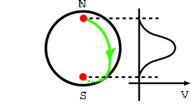
Figure 2: ${\bf C}P^{1}$ and the potential $V$. The base space of $T^{*}{\bf C}P^{1}$, ${\bf C}P^{1}\simeq S^{2}$, is displayed. This model contains two discrete vacua denoted by $N$ and $S$. The potential $V$ is also displayed on the right of the ${\bf C}P^{1}$. It admits a single wall solution connecting these two vacua expressed by a curve. The $U(1)$ isometry around the axis connecting $N$ and $S$ is spontaneously broken by the wall configuration.

From the target manifold (3.76) one can easily see that there exists a duality between theories with the same flavor and two different gauge groups in the case of the infinite gauge coupling [34, 17]:

$$U(N_{\rm C})\leftrightarrow U(\tilde{N}_{\rm C})=U(N_{\rm F}-N_{\rm C})\,.$$ (3.77)

This duality holds for the Lagrangian of the nonlinear sigma models, and leads to the duality of the BPS equations between these two theories. The BPS equation for a dual theory is discussed in Appendix D. This duality holds also for the moduli space of domain wall configurations.

3.7 Factorizable Moduli and Solutions with Finite Coupling

If the moduli matrix $H_{0}$ takes a certain restricted form which will be defined below as the ‘$U(1)$-factorizable moduli’, the BPS equation (3.13) for our non-Abelian case can be decomposed into a direct sum of BPS equations for the Abelian case. In such circumstances, we can construct exact solutions for finite, but special values of gauge coupling by using the solutions found in our previous paper [15].

The BPS equation (3.13) is covariant under the world-volume transformation (3.6), where the matrix $H_{0}e^{2My}H_{0}{}^{\dagger}$ transforms with multiplication of constant matrices $V$ and $V^{\dagger}$ from both sides of this matrix. The world-volume symmetry allows us to make this matrix $H_{0}e^{2My}H_{0}{}^{\dagger}$ diagonal at one point of the extra dimension, say, $y=y_{0}$. If the matrix $H_{0}e^{2My}H_{0}{}^{\dagger}$ with this gauge fixing remains diagonal at every other points in the extra dimension $y\not=y_{0}$,

$$H_{0}e^{2My}H_{0}{}^{\dagger}=c\,{\rm diag.}\left({\cal W}_{1}(y),{\cal W}_{2}(y),\cdots,{\cal W}_{N_{\rm C}}(y)\right),$$ (3.78)

then, we call that moduli matrix $H_{0}$ as ‘$U(1)$-factorizable’. Note that such a property is a characteristic inherent in each moduli matrix $H_{0}$, and is independent of the choice of the initial coordinate $y_{0}$. Thus the $U(1)$-factorizability is a property intrinsically attached to each point on the moduli manifold of the BPS solution. If the moduli matrix is $U(1)$-factorizable, off-diagonal components of the matrix $H_{0}e^{2My}H_{0}{}^{\dagger}$ vanishes at any point of the extra dimension $y$ by definition. This implies that each coefficient of $e^{2m_{A}y}$ in the off-diagonal components must vanish. We consider in this paper the case of non-degenerate masses, unless otherwise stated. In the non-degenerate case, the condition for the $U(1)$-factorizability can be written for each flavor $A$

$$(H_{0})^{rA}\left((H_{0}{})^{sA}\right)^{*}=0,\quad{\rm for~{}}r\not=s,$$ (3.79)

where we do not take sum over the flavor indices $A$. In other words, $(H_{0})^{rA}$ can be non-vanishing in only one color component $r$ for each flavor $A$. For instance, we can choose $H_{0}$ as

$$H_{0}=\sqrt{c}\left(\begin{array}[]{ccccc}0&0&e^{r_{3}}&0&\\ 0&0&0&0&\cdots\\ 0&e^{r_{2}}&0&e^{r_{4}}&\\ e^{r_{1}}&0&0&0&\\ &\vdots&&&\ddots\end{array}\right).$$ (3.85)

We can rearrange these moduli matrix to a standard form (an echelon form) in Eq. (3.3) with the world-volume symmetry keeping the forms (3.78),(3.79). Moduli matrices representing points of $U(1)$-factorizable moduli do not always satisfy the condition (3.79), because of the redundancy of the world- volume symmetry. We can always establish the $U(1)$-factorizability of moduli matrices by checking the condition (3.79) in the standard form.

For such a $U(1)$-factorizable moduli, it is sufficient to take an ansatz where only the diagonal components of the matrix $\Omega$ survive

$$\Omega={\rm diag.}\left(e^{2\psi_{1}},\,e^{2\psi_{2}},\,\cdots,e^{2\psi_{N_{\rm C}}}\right),$$ (3.86)

where $\psi_{r}(y)$’s are real functions. With this ansatz, the BPS equations (3.13) for the non-Abelian gauge theories with the $U(1)$-factorizable moduli with the condition (3.78) reduce to a set of the BPS equations [25, 14] for the Abelian gauge theory

$$\partial_{y}^{2}\psi_{r}={g^{2}c\over 2}\left(1-e^{-2\psi_{r}}{\cal W}_{r}\right),\qquad{\rm for~{}}r=1,2,\cdots N_{\rm C},$$ (3.87)

where the functions ${\cal W}_{r}$ defined in (3.78) are given by

$${\cal W}_{r}=\sum_{A\in{\cal A}_{r}}e^{2m_{A}y+2r_{A}}.$$ (3.88)

${\cal A}_{r}$ is a set of flavors of the hypermultiplet scalars whose $r$-th color component is non-vanishing. Note that the condition (3.79) of the $U(1)$-factorizability can be rewritten as ${\cal A}_{r}\cap{\cal A}_{s}=\phi$ for $r\not=s$. In this case, the vector multiplet scalars $\Sigma$ and the hypermultiplet scalars $H^{1rA}$ are given by [14]

$$\Sigma={\rm diag.}\left(\partial_{y}\psi_{1},\,\partial_{y}\psi_{2},\,\cdots,\,\partial_{y}\psi_{N_{\rm C}}\,\right),$$ (3.89)

$$H^{1rA}=\sqrt{c}e^{-\psi_{r}(y)+m_{A}(y-y_{0})+r_{A}},$$ (3.90)

with a gauge choice of $W_{y}=0$. The energy density ${\cal E}$ of the BPS multi-walls in Eq.(2.44) are obtained by a summation of energy density for each individual wall $c\partial_{y}^{2}\psi_{r}$ as

$${\cal E}=c\,\partial_{y}{\rm Tr}(\Sigma)=c\sum_{r=1}^{N_{\rm C}}\partial^{2}_{y}\psi_{r}.$$ (3.91)

Therefore, the profile of the energy density for the BPS multi-walls are obtained by a simple summation of those of individual wall generated from different $\psi_{r}$. Since moduli parameters contained in the BPS equation (3.87) for each $\psi_{r}$ are independent of each other, we find that the walls originated in different $\psi_{r}$ can have positive and negative relative positions other maintaining their identity. When two walls can go through each other like here, they are called penetrable each other. More generally, if we take up two sets of walls belonging to two diagonal entries of Eq. (3.89) of the $U(1)$-factorizable case, these two sets are mutually penetrable, in the sense that they can go through each other provided the relative distances between walls in the same diagonal entry are fixed.

We have found previously that the $U(1)$ gauge theories allow exact BPS solutions for finite gauge couplings [14]. These finite gauge couplings have been found to be restricted to specific values in relation to mass splittings: exact solutions for single-walls at $g^{2}c=4(m_{1}-m_{2})^{2}/k^{2}$, for $k=2,3,4$, and double wall at $g^{2}c=(m_{1}-m_{2})^{2}=(m_{2}-m_{3})^{2}$. A number of exact solutions of the BPS multi-walls for our non-Abelian gauge theory can be obtained in the $U(1)$-factorizable cases by embedding these known solutions into the equations (3.87) for the $U(1)$ factor groups. For example, in the case of $N_{\rm C}=2,\,N_{\rm F}=4$ with

$$g^{2}c=(\Delta m)^{2},\quad m_{1}-m_{2}=m_{3}-m_{4}\equiv\Delta m,$$ (3.92)

and with a $U(1)$-factorizable moduli matrix

$$H_{0}=\sqrt{c}\left(\begin{array}[]{ccccc}e^{-m_{1}y_{1}}&e^{-m_{2}y_{1}}&0&0\\ 0&0&e^{-m_{3}y_{2}}&e^{-m_{4}y_{2}}\end{array}\right)$$ (3.95)

with real parameters $y_{1},\ y_{2}$. Then an exact solution is given by two copies of the solution for $k=2$ as

$$\psi_{1} = \log\left(e^{m_{1}(y-y_{1})}+e^{m_{2}(y-y_{1})}\right),\quad$$

$$\psi_{2} = \log\left(e^{m_{3}(y-y_{2})}+e^{m_{4}(y-y_{2})}\right).$$ (3.96)

This solution represents a double wall that are located at $y=y_{1}$ and $y=y_{2}$. More complicated exact solutions can be obtained if we take a larger number of flavor and color. For instance, in the case of $N_{\rm C}=3,\,N_{\rm F}=7$ with

$$g^{2}c=4m^{2},\ M={\rm diag.}\left(2m,\,{3\over 2}m,\,m,\,0,\,-m,\,-{3\over 2}m,\,-2m\right)\quad$$ (3.97)

and with a $U(1)$-factorizable moduli matrix

$$H_{0}=\sqrt{c}\left(\begin{array}[]{ccccccc}e^{-2my_{1}}&0&0&e^{mR}&0&0&e^{2my_{1}}\\ 0&0&e^{-my_{2}}&0&e^{my_{2}}&0&0\\ 0&e^{-{3\over 2}my_{3}}&0&0&0&e^{-{3\over 2}my_{3}}&0\end{array}\right),\quad$$ (3.101)

we obtain an exact solution for a BPS four-walls

$$\psi_{1} = \log\left(e^{2m(y-y_{1})}+e^{-2m(y-y_{1})}+\sqrt{6+e^{2mR}}\right),$$

$$\psi_{2} = \log\left(e^{m(y-y_{2})}+e^{-m(y-y_{2})}\right),\quad$$

$$\psi_{3} = {3\over 2}\log\left(e^{m(y-y_{3})}+e^{-m(y-y_{3})}\right).$$ (3.102)

Although we have given only the solution for $\psi$, the vector multiplet scalar $\Sigma$ and the hypermultiplet scalar $H^{1}$ can be obtained readily from $\psi$ by using Eqs. (3.89) and (3.90).

4 Constructing Explicit Solutions at Infinite Coupling

In this section, as explicit examples, we construct BPS wall solutions and investigate their properties in the $N_{\rm C}=2$, $N_{\rm F}=3,4$ cases. General $N_{\rm C}$ and/or $N_{\rm F}$ cases are similar. In the first subsection, we work with the simplest case of $N_{\rm C}=2,\ N_{\rm F}=3$ to illustrate methods to construct the solutions and relations between the moduli matrices $H_{0}$ and profiles of solutions for domain walls. This case is, however, equivalent to the case of $N_{\rm C}=1,\,N_{\rm F}=3$ by duality $N_{\rm C}\leftrightarrow\tilde{N}_{\rm C}$, and thus the properties of walls are also equivalent to the Abelian case. In the second subsection, we consider the case of $N_{\rm C}=2,\,N_{\rm F}=4$, which is the simplest case that possesses characteristic properties of genuine non-Abelian walls. We will define matrix operators acting on the moduli space to create multi-wall solutions from a solution with walls less by one.

4.1 $N_{\rm C}=2,\ N_{\rm F}=3$ Case

In this case, there exist $3(={}_{3}C_{2})$ vacua and maximally $2(=N_{\rm C}\tilde{N}_{\rm C})$ walls interpolating between these vacua. Fig. 3 illustrates the diagram of SUSY vacua and walls in the space of the scalars of vector multiplets $\Sigma$. Let us construct explicit expressions of the exact solutions for the BPS equations. First of all, it is important to classify arbitrary $2\times 3$ moduli matrices $H_{0}$ in the standard form (3.3) into several types of matrices. The standard form matrices

$$H_{0\langle 12\rangle}=\sqrt{c}\left(\begin{array}[]{ccc}1&0&0\\ 0&1&0\end{array}\right),\ \ H_{0\langle 13\rangle}=\sqrt{c}\left(\begin{array}[]{ccc}1&0&0\\ 0&0&1\end{array}\right),\ \ H_{0\langle 23\rangle}=\sqrt{c}\left(\begin{array}[]{ccc}0&1&0\\ 0&0&1\end{array}\right)$$ (4.7)

correspond to the three vacua $\langle 12\rangle,\langle 13\rangle$ and $\langle 23\rangle$, respectively as illustrated in Fig. 3. The three matrices with complex parameters $r_{1},\,r_{2}$ and $r_{3}$,

$$H_{0}{}_{\langle 12\leftarrow 13\rangle} = \sqrt{c}\left(\begin{array}[]{ccc}1&0&0\\ 0&1&e^{r_{1}}\end{array}\right),\quad-\infty<{\rm Re}(r_{1})<\infty,$$ (4.10)

$$H_{0}{}_{\langle 13\leftarrow 23\rangle} = \sqrt{c}\left(\begin{array}[]{ccc}1&e^{r_{2}}&0\\ 0&0&1\end{array}\right),\quad-\infty<{\rm Re}(r_{2})<\infty,$$ (4.13)

$$H_{0}{}_{\langle 12\leftarrow 32\rangle} = \sqrt{c}\left(\begin{array}[]{ccc}1&0&e^{r_{3}}\\ 0&1&0\end{array}\right),\quad-\infty<{\rm Re}(r_{3})<\infty$$ (4.16)

describe single-wall configurations, where the suffix $\langle A_{1}A_{2}\leftarrow B_{1}B_{2}\rangle$ denotes a moduli matrix describing a BPS state interpolating from the vacuum $\langle B_{1}B_{2}\rangle$ at $y=-\infty$ to the vacuum $\langle A_{1}A_{2}\rangle$ at $y=+\infty$ . By these labels, we recognize the first two of the matrices (4.16) describe elementary walls and the last one a compressed wall of level one as defined in (3.53). As explained in Sec. 3.5, positions $y_{1},y_{2}$ and $y_{3}$ of the single-walls labeled by $\langle 12\leftarrow 13\rangle,\langle 13\leftarrow 23\rangle$ and $\langle 12\leftarrow 32\rangle$ can be guessed roughly as

$$y_{1} \equiv {{\rm Re}(r_{1})\over m_{2}-m_{3}},\quad y_{2}\equiv{{\rm Re}(r_{2})\over m_{1}-m_{2}},\quad y_{3}\equiv{{\rm Re}(r_{3})\over m_{1}-m_{3}},$$ (4.17)

respectively. Finally, the moduli matrix

$$H_{0}{}_{\langle 12\leftarrow 23\rangle} = \sqrt{c}\left(\begin{array}[]{ccc}1&e^{r_{2}}&0\\ 0&1&e^{r_{1}}\end{array}\right),\quad-\infty<{\rm Re}(r_{1})<\infty,\quad-\infty<{\rm Re}(r_{2})<\infty$$ (4.20)

corresponds to a double wall interpolating from the vacuum $\langle 23\rangle$ to the vacuum $\langle 12\rangle$ through the vicinity of the vacuum $\langle 13\rangle$. Note that we have distinguished the moduli matrix (4.20) from the third one in Eq. (4.16) by their orders of flavors. As described in Sec. 2.3, it is convenient to distinguish the vacua with different order of labels. This is because there are no freedom of local gauge transformation, if we fix the gauge by eliminating the off-diagonal components of the scalar $\Sigma$. In that gauge, the labels for moduli matrices reflect trajectories in the space of the diagonal components $(\Sigma^{0},\Sigma^{3})$ as illustrated in Fig. 3. This is the most convenient gauge to represent the solutions, which we usually use. Various types of walls are distinguished by arrows as explained in Fig. 4.

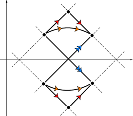
Figure 3: Walls for $N_{\rm C}=2$ and $N_{\rm F}=3$. This model admits three single walls. Two of them are elementary walls and the other is a compressed wall. The latter is obtained in a particular limit of the double wall configuration. Meaning of arrows is explained in Fig. 4.

Figure 4: An arrow with a single arrowhead denotes an elementary wall. An arrow with duplicate ($l$-uninterrupted) arrowhead denotes a compressed wall of level $1$ ($l-1$). An arrow with two separate arrowheads denotes a double wall consisting of two single walls with the relative distance as a moduli.

The above identification between moduli matrices and BPS objects are performed without constructing the exact solutions. It is also easy to investigate relations between these moduli matrices. For instance, the moduli matrix $H_{0}{}_{\langle 12\leftarrow 23\rangle}$ approaches $H_{0}{}_{\langle 12\leftarrow 13\rangle}$ in the limit of $r_{2}\rightarrow-\infty$. Since $y=y_{2}$ corresponds to the position of the wall interpolating between $\langle 23\rangle$ and $\langle 13\rangle$, $r_{2}\rightarrow-\infty$ implies expelling the wall to negative infinity $y_{2}\rightarrow-\infty$. This explains $H_{0}{}_{\langle 12\leftarrow 23\rangle}\rightarrow H_{0}{}_{\langle 12\leftarrow 13\rangle}$ in the limit of $r_{2}\rightarrow-\infty$. The moduli matrices $H_{0}{}_{\langle 12\leftarrow 32\rangle}$ for single-wall and $H_{0}{}_{\langle 12\leftarrow 23\rangle}$ for double wall describe BPS states interpolating between the same pair of the vacua at the boundaries, in other words these moduli matrices describes different submanifolds of the same topological sector. To understand how these submanifold connect with each others, it is convenient to consider these moduli matrices in the row-reduced echelon form (3.33). Let us perform the world-volume symmetry transformation (3.6) on the $H_{0\langle 12\leftarrow 23\rangle}$ so that the moduli matrix becomes a row-reduced echelon form.

$$H_{0\langle 12\leftarrow 23\rangle} \rightarrow \left(\begin{array}[]{cc}1&-e^{r_{2}}\\ 0&1\end{array}\right)H_{0\langle 12\leftarrow 23\rangle}=\sqrt{c}\left(\begin{array}[]{ccc}1&0&-e^{r_{1}+r_{2}}\\ 0&1&e^{r_{1}}\end{array}\right).$$ (4.25)

Here, if we take the limit of $r_{1}\rightarrow-\infty$, keeping the parameter

$$r_{3}=r_{1}+r_{2}+\pi i$$ (4.26)

finite ($r_{2}\rightarrow\infty$), we find that $H_{0\langle 12\leftarrow 23\rangle}$ in the row-reduced echelon form becomes $H_{0}{}_{\langle 12\leftarrow 32\rangle}$. This relation between $H_{0\langle 12\leftarrow 23\rangle}$ and $H_{0}{}_{\langle 12\leftarrow 32\rangle}$ is quite different from that between $H_{0\langle 12\leftarrow 23\rangle}$ and $H_{0}{}_{\langle 12\leftarrow 13\rangle}$, while one describes a double wall and the other describes a single wall in the both case. Since the boundary conditions are not changed by transition form $H_{0\langle 12\leftarrow 23\rangle}$ to $H_{0}{}_{\langle 12\leftarrow 32\rangle}$ in this case, the transition means that the two walls approach each other and are compressed to a single wall. In the region of $y_{1}\leq y_{2}$, a profile of the energy density of two constituent walls are compressed into a profile of a single peak. The parameters $y_{1}$ and $y_{2}$ do not represent positions of the walls. Instead, the parameter $y_{1}-y_{2}$ represents the extent of compression of the walls. The relation (4.26) implies the parameter $y_{3}$, which denotes the position of the single wall labeled by $\langle 12\leftarrow 32\rangle$, is related to the center of mass of the double wall formally

$$y_{3}={T_{\langle 2\leftarrow 3\rangle}y_{1}+T_{\langle 1\leftarrow 2\rangle}y_{2}\over T_{\langle 2\leftarrow 3\rangle}+T_{\langle 1\leftarrow 2\rangle}}.$$ (4.27)

We will discuss this compression of walls more using an exact solution in the latter part of this subsection. This phenomenon of compressed wall has also occurred in the Abelian case [24, 25, 14]. Actually, we find that this $N_{\rm C}=2,N_{\rm F}=3$ case is dual to the $N_{\rm C}=1,N_{\rm F}=3$ case, which is the case of the Abelian gauge theory.

Now let us construct exact solutions explicitly with the infinite gauge coupling by the formula for solutions (3.71) and discuss the behavior of solutions. As our first example, let us start with solutions for the moduli matrices $H_{0\langle 12\leftarrow 13\rangle}$ to confirm that $H_{0\langle 12\leftarrow 13\rangle}$ in fact gives a domain wall interpolating between SUSY vacua ${\langle 13\rangle}$ and ${\langle 12\rangle}$. Note that the moduli matrix $H_{0}{}_{\langle 12\leftarrow 13\rangle}$ are $U(1)$-factorizable and the $\Omega$ for above $H_{0}{}_{\langle 12\rangle}$ calculated by (3.71) forms a diagonal matrix, thus we can easily find $S$ as

$$S_{\langle 12\leftarrow 13\rangle} = \left(\begin{array}[]{cc}e^{m_{1}y}&0\\ 0&\sqrt{e^{2m_{2}y}+e^{2m_{3}y+2{\rm Re}(r_{1})}}\end{array}\right),$$ (4.30)

where we take the easiest gauge choice. Therefore, from (3.5), we obtain the following single wall solution

$$H^{1}=\sqrt{c}\left(\begin{array}[]{ccc}1&0&0\\ 0&\frac{e^{m_{2}(y-y_{1})}}{\sqrt{e^{2m_{2}(y-y_{1})}+e^{2m_{3}(y-y_{1})}}}&\frac{e^{m_{3}(y-y_{1})+i{\rm Im}(r_{1})}}{\sqrt{e^{2m_{2}(y-y_{1})}+e^{2m_{3}(y-y_{1})}}}\end{array}\right),$$ (4.33)

where ${\rm Im}(r_{1})$ is a moduli with respect to broken $U(1)_{\rm F}$-phase. $\Sigma$ and $W_{y}$ can also be calculated from $S$ as

$$\Sigma+iW_{y}=\left(\begin{array}[]{cc}m_{1}&0\\ 0&\frac{m_{2}e^{2m_{2}(y-y_{1})}+m_{3}e^{2m_{3}(y-y_{1})}}{e^{2m_{2}(y-y_{1})}+e^{2m_{3}(y-y_{1})}}\end{array}\right),$$ (4.36)

The components $\Sigma^{0},\ \Sigma^{3}$ read

$$\Sigma^{0} = m_{1}+\frac{m_{2}e^{2m_{2}(y-y_{1})}+m_{3}e^{2m_{3}(y-y_{1})}}{e^{2m_{2}(y-y_{1})}+e^{2m_{3}(y-y_{1})}},$$

$$\Sigma^{3} = m_{1}-\frac{m_{2}e^{2m_{2}(y-y_{1})}+m_{3}e^{2m_{3}(y-y_{1})}}{e^{2m_{2}(y-y_{1})}+e^{2m_{3}(y-y_{1})}},$$ (4.37)

while $\Sigma^{1},\,\Sigma^{2}$ and $W_{y}$ vanish due to the $U(1)$-factorizability of the moduli matrix $H_{0}{}_{\langle 13\rightarrow 12\rangle}$. These wall solution for $\Sigma^{0},\,\Sigma^{3}$ and $H_{0}$ are illustrated in Fig. 5.

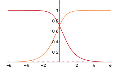
Figure 5: Configurations for $\Sigma^{0},\Sigma^{3}$ and $(H^{1})^{22},(H^{1})^{23}$, in the case of $(m_{1},\,m_{2},\,m_{3})=(1,0,-1)$ and $r_{1}=0$.

From these solutions, we confirm that the parameter $y_{1}$ defined by (4.17) is really the position of the wall in this case. The configuration approaches to the vacuum $\langle 13\rangle$ in the limit $y\rightarrow-\infty$

$$H^{1}=\sqrt{c}\left(\begin{array}[]{ccc}1&0&0\\ 0&0&1\end{array}\right),\quad\Sigma=\left(\begin{array}[]{cc}m_{1}&0\\ 0&m_{3}\end{array}\right),$$ (4.42)

and to the vacuum $\langle 12\rangle$ in the limit $y\rightarrow\infty$

$$H^{1}=\sqrt{c}\left(\begin{array}[]{ccc}1&0&0\\ 0&1&0\end{array}\right),\quad\Sigma=\left(\begin{array}[]{cc}m_{1}&0\\ 0&m_{2}\end{array}\right).$$ (4.47)

Moreover $\Sigma^{0}+\Sigma^{3}=2m_{1}$ implies that this one wall solution follows a straight line from ${\langle 13\rangle}$ to ${\langle 12\rangle}$ in the $(\Sigma^{0},\Sigma^{3})$-plane when $y$ varies from $-\infty$ to $+\infty$, as shown in Fig. 3. Generally, we find that the configuration of the solution for single wall is a straight line segment linking two vacua in the $(\Sigma^{0},\,\Sigma^{3})$-plane with the gauge choice of $\Sigma^{1}=\Sigma^{2}=0$.

The solution for the $H_{0}{}_{\langle 12\leftarrow 23\rangle}$ describing two walls can be obtained similarly. We are, however, faced with a little technical problem in this case. Substituting the explicit form of the moduli matrix (4.20) into the formula (3.71), we obtain

$$\Omega=\left(\begin{array}[]{cc}e^{2m_{1}y}+e^{2m_{2}y+2{\rm Re}(r_{2})}&e^{2m_{2}y+r_{2}}\\ e^{2m_{2}y+r_{2}^{*}}&e^{2my_{2}y}+e^{2m_{3}y+2{\rm Re}(r_{1})}\end{array}\right),$$ (4.50)

and hence, off-diagonal components appear. Therefore, we should consider the general case where $\Omega=SS^{\dagger}$ is given by

$$\Omega=SS^{\dagger}=\left(\begin{array}[]{cc}\omega_{+}&\omega_{0}^{*}\\ \omega_{0}&\omega_{-}\end{array}\right),$$ (4.53)

with $\omega_{\pm}\in\mathbf{R},\ \omega_{0}\in\mathbf{C}$. Since the $U(2)$ gauge symmetry can be fixed by choosing $S$ to be a lower triangular matrix, we obtain an explicit form of the matrix $S$

$$S = \left(\begin{array}[]{cc}\sqrt{\omega_{+}}&0\\ \frac{\omega_{0}}{\sqrt{\omega_{+}}}&\frac{\sqrt{\omega_{+}\omega_{-}-|\omega_{0}|^{2}}}{\sqrt{\omega_{+}}}\end{array}\right).$$ (4.56)

Although this gauge choice is appropriate to obtain an explicit form of the matrix $S$ from $\Omega$, it is not convenient to understand physics of walls since the off-diagonal part of both the vector multiplet scalars and the gauge fields are non-vanishing, $\Sigma^{I}\not=0,\,W_{y}\not=0$ in this gauge. We can, however, calculate the gauge-invariant quantities without the above explicit form of the matrix $S$ as we explained in Sec. 3.1. For simplicity, we set $M={\rm diag.}(m,\,0,\,-m),$ and $(r_{1},r_{2})=(mR/2+i\theta/2,-mR/2-i\theta/2)$, then the solutions for the scalar $\Sigma$ are obtained by the formula (3.17) and (3.20)

$$\Sigma^{0} = m{e^{2my}-e^{-2my}\over e^{2my}+e^{-2my}+e^{mR}}\sim\left\{\begin{array}[]{cc}\pm m,&2|y|\gg R,\quad y=\pm|y|\\ 0,&2|y|\ll R\end{array}\right.$$ (4.59)

$$|\Sigma| = 2m{\sqrt{(\cosh({2my})+e^{mR})^{2}-1}\over e^{2my}+e^{-2my}+e^{mR}}\sim\left\{\begin{array}[]{cc}m,&2|y|\gg R\\ 2m,&2|y|\ll R\end{array}\right.,$$ (4.62)

where $R$ represents the distance between the two walls if $R>0$. Configurations with several values of $R$ for this solution are illustrated in the $(\Sigma^{0},\Sigma^{3})$-plane with the gauge choice $\Sigma^{1}=\Sigma^{2}=0$ in Fig. 6, whereas a configuration corresponding to the $H_{0}{}_{\langle 12\leftarrow 32\rangle}$ is a straight line segment through the origin of the coordinate axis from $\langle 32\rangle(\not=\langle 23\rangle)$ to $\langle 12\rangle$ in the same gauge $\Sigma^{1}=\Sigma^{2}=0$.

Figure 6: Configuration for the double wall with $m=1,$ $R=3,0,-3$ and $c=1$. Fig. a) are paths of the solutions in the $(\Sigma^{0},\Sigma^{3})$-plane and Fig. b) are energy densities, ${\cal E}=(c/2)\partial_{y}^{2}{\rm log}({\rm det}\Omega)$. Note that the trajectory for $R<0$ passes through the vicinity of the point $(\Sigma^{0},\Sigma^{3})=(0,0)$, which is not vacuum, while the trajectory for $R>0$ passes through the vicinity of the vacuum $\langle 13\rangle$.

The difference between profiles of these solutions can be understood as follows. If we allow local gauge transformations to eliminate the off-diagonal components $\Sigma^{1},\Sigma^{2}$, we can rotate a vector $\vec{\Sigma}$ by $\pi$ around the $T^{1}$ axis only in a region of $y\ll 0$ so that the sign of $\Sigma^{3}$ is flipped. This interpretation can be strengthened by examining the gauge invariant quantity $I_{\rm gauge}$ in Eq. (3.19). While $I_{\rm gauge}$ for single wall vanishes, it is nontrivial for the double wall

$$I_{\rm gauge} = 4m^{2}e^{mR}{e^{2my}+e^{-2my}+e^{mR}\over((\cosh({2my})+e^{mR})^{2}-1)^{2}}\sim\left\{\begin{array}[]{cc}16m^{2}e^{-m(6|y|-R)},&2|y|\gg R\\ 4m^{2}e^{-2mR},&2|y|\ll R\end{array}\right..$$ (4.65)

Figure 7: Configuration of $\sqrt{I_{\rm gauge}}$ with $m=1$ $R=10,\,R=-10$. If we take the gauge $\Sigma^{1}=\Sigma^{2}=0$ and set $\theta=0$, then $\sqrt{I_{\rm gauge}}=W_{y}^{1}$ and $W_{y}^{2}=0$. Note that scales of the two figures are quite different. We find that a profile for $R\gg 0$ is a quite low plateau which has edges on the double wall, and a profile for $R\ll 0$ approaches to a delta function on the compressed single wall.

In the limit of $R\rightarrow-\infty$, a profile of $\sqrt{I_{\rm gauge}}$ approaches to a delta function as illustrated in Fig.7

$$\lim_{R\rightarrow-\infty}\sqrt{I_{\rm gauge}}=\pi\delta(y),$$ (4.66)

where the factor $\pi$ is obtained by integrating over the whole region of the coordinate $y$. Usually we use the gauge where $\Sigma^{1}=\Sigma^{2}=0,W_{y}^{3}=0$ unless otherwise stated. In that gauge the gauge invariant quantity is expressed in terms of gauge fields as in Eq.(3.22). Since the gauge invariant quantity $\sqrt{I_{\rm gauge}}$ can then be interpreted as $W_{y}^{1}=\pi\delta(y)$, we can devise a local gauge transformation to eliminate the $W_{y}^{1}$. The gauge transformation which fixes the boundary condition at $y=\infty$ is given by a step function $\Lambda(y)=\pi\Theta(-y)$

$$W_{y}^{1}\rightarrow W_{y}^{1^{\prime}}=W_{y}^{1}+\partial_{y}\Lambda(y)=0.$$ (4.67)

The resulting configuration turns out to be

$$\Sigma^{1^{\prime}}=\Sigma^{2^{\prime}}=0,\quad\Sigma^{3^{\prime}}=\Sigma^{3}\epsilon(y)\quad W_{y}^{1^{\prime}}=W_{y}^{2^{\prime}}=W_{y}^{3^{\prime}}=0$$ (4.68)

where $\epsilon(y)$ is a sign function. By this singular gauge transformation, a wall solution represented by a segment broken at $\Sigma^{0}=|\Sigma|=0$ is transformed to a straight line segment which is generated by the third matrix in (4.16). The result (4.66) appears to differ from the result $I_{\rm gauge}=0$ calculated from the moduli matrix $H_{0}{}_{\langle 12\leftarrow 32\rangle}$, in spite of the gauge-invariance of $I_{\rm gauge}$. This apparent discrepancy is due to the fact that $I_{\rm gauge}$ is ill-defined just at the point $|\Sigma|=0$.

We summarize all the topological sectors and the associated moduli matrices in the case of $N_{\rm C}=2,\,N_{\rm F}=3$ in Table 1.

Table 1: Six topological sectors in the case of $N_{\rm C}=2,\,N_{\rm F}=3$. $a_{1}$ and $a_{2}$ are matrices which generate wall configuration as will be explained in the next subsection.

top. sector	moduli matrix	dim.	objects
$\langle 12\rangle\leftarrow\langle 12\rangle$	$H_{0}{}_{\langle 12\rangle}$	0	vacuum $\langle 12\rangle$
$\langle 13\rangle\leftarrow\langle 13\rangle$	$H_{0}{}_{\langle 13\rangle}$	0	vacuum $\langle 13\rangle$
$\langle 23\rangle\leftarrow\langle 23\rangle$	$H_{0}{}_{\langle 23\rangle}$	0	vacuum $\langle 23\rangle$
$\langle 12\rangle\leftarrow\langle 13\rangle$	$H_{0}{}_{\langle 12\leftarrow 13\rangle}$	2	elementary wall $a_{2}$
$\langle 13\rangle\leftarrow\langle 23\rangle$	$H_{0}{}_{\langle 13\rightarrow 23\rangle}$	2	elementary wall $a_{1}$
$\langle 12\rangle\leftarrow\langle 23\rangle$	$H_{0}{}_{\langle 12\rightarrow 23\rangle}\oplus H_{0}{}_{\langle 12\rightarrow 32\rangle}$	4	double wall $(a_{1},a_{2})\oplus$ compressed wall $a_{1}a_{2}$

4.2 $N_{\rm C}=2,\ N_{\rm F}=4$ Case

The $N_{\rm C}=2,\ N_{\rm F}=4$ case is the simplest example containing characteristic properties originated from a non-Abelian gauge group. In this case, there are six SUSY vacua, and six elementary walls interpolating between these vacua. There exist 20 BPS topological sectors described by 25 kinds of moduli matrices in the standard form, which we show explicitly in Appendix F. Note that if we choose an arbitrary set of vacua at both boundaries, we find that there are 21 topological sectors, that is, there exists one non-BPS topological sector, which interpolates between vacua $\langle 14\rangle$ and $\langle 23\rangle$. If we consider the maximal topological sector interpolating between vacua $\langle 12\rangle$ and $\langle 34\rangle$, the moduli space is described by four complex moduli parameters, of which four real parameters represent positions of four walls, and other four real parameters represent the orientation of walls in the target space. Among them, relative phase of vacua separated by the wall can be understood as the Nambu-Goldstone mode. We will also obtain one moduli parameter which cannot be attributed to the spontaneously broken symmetry, namely the quasi-Nambu-Goldstone mode.

All single walls including elementary walls and compressed walls are displayed in Fig. 8.

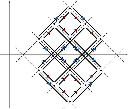
Figure 8: All single walls for $N_{\rm C}=2$ and $N_{\rm F}=4$. Lines with a single arrow are elementary walls, whereas lines with a double (triple) arrow are compressed single walls of level one (two).

Multi-wall solutions are displayed in Fig. 9.

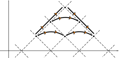
Figure 9: Multi-walls. a) All double wall configurations composed of two elementary walls are displayed. b) Examples of triple-wall and the four-wall configurations in the maximal topological sector are displayed.

A remarkable phenomenon in this case is that there exists a pair of walls whose positions can commute with each other. Let us show this property, considering the topological sector labeled by $\langle 13\rangle\leftarrow\langle 24\rangle$. A moduli matrix for this sector $H_{0\langle 13\leftarrow 24\rangle}$ is given by two complex moduli parameters $r_{2},r_{3}$ by

$$H_{0\langle 13\leftarrow 24\rangle}=\sqrt{c}\left(\begin{array}[]{cccc}1&e^{r_{3}}&0&0\\ 0&0&1&e^{r_{2}}\end{array}\right).$$ (4.71)

We notice that this moduli matrix is $U(1)$-factorizable, and a solution obtained with this moduli matrix is given by

$$\Sigma^{0}+\Sigma^{3} = {m_{1}e^{2m_{1}y}+m_{2}e^{2m_{2}y+2{\rm Re}(r_{3})}\over e^{2m_{1}y}+e^{2m_{2}y+2{\rm Re}(r_{3})}},$$

$$\Sigma^{0}-\Sigma^{3} = {m_{3}e^{2m_{3}y}+m_{4}e^{2m_{4}y+2{\rm Re}(r_{2})}\over e^{2m_{3}y}+e^{2m_{4}y+2{\rm Re}(r_{2})}}$$ (4.72)

and $\Sigma^{1}=\Sigma^{2}=W_{y}=0$, and

$$H^{1}=\sqrt{c}\left(\begin{array}[]{cccc}{e^{m_{1}y}\over\sqrt{e^{2m_{1}y}+e^{2m_{2}y+2{\rm Re}(r_{3})}}}&{e^{m_{2}y+r_{3}}\over\sqrt{e^{2m_{1}y}+e^{2m_{2}y+2{\rm Re}(r_{3})}}}&0&0\\ 0&0&{e^{m_{3}y}\over\sqrt{e^{2m_{3}y}+e^{2m_{4}y+2{\rm Re}(r_{2})}}}&{e^{m_{4}y+r_{2}}\over\sqrt{e^{2m_{3}y}+e^{2m_{4}y+2{\rm Re}(r_{2})}}}\end{array}\right).$$ (4.75)

Profiles of $\Sigma^{0}\pm\Sigma^{3}$ and $H^{1}$ are illustrated in Fig. 10.

Figure 10: Penetrable walls of $\langle 13\leftarrow 24\rangle$ in $N_{\rm C}=2$, $N_{\rm F}=4$ case. $M={\rm diag.}({3\over 2},{1\over 2},-{1\over 2},-{3\over 2})$. a) $r_{3}=5,\,r_{2}=-5$: the intermediate region shows $\langle 23\rangle$ vacuum. b) $r_{3}=-5,\,r_{2}=5$, $c=1$: the intermediate region shows $\langle 14\rangle$ vacuum.

This solution describes a configuration of double wall. In this case, position of the walls are exactly expressed by

$$y_{3}={{\rm Re}(r_{3})\over m_{1}-m_{2}},\quad y_{2}={{\rm Re}(r_{2})\over m_{3}-m_{4}}.$$ (4.77)

In a region $y_{2}>y_{3}$, the configuration interpolates between vacua $\langle 13\rangle$ and $\langle 24\rangle$ through the vicinity of the vacuum $\langle 14\rangle$. The wall at $y_{2}$ ($y_{3}$) interpolates between vacua $\langle 13\rangle$ and $\langle 14\rangle$ ($\langle 24\rangle$ and $\langle 14\rangle$). On the other hand, in a region $y_{3}>y_{2}$ the wall at $y_{3}$ ($y_{2}$) interpolates as $\langle 13\rangle\leftarrow\langle 23\rangle$ ($\langle 23\rangle\leftarrow\langle 24\rangle$). Note that while intermediate vacua are different from one region $(y_{3}>y_{2})$ to the other $(y_{3}<y_{2})$, the two parameters $y_{2},y_{3}$ retain the physical meaning as positions of the walls, in contrast to the example of the compressed wall in the last subsection. The wall represented by the position $y_{2}$ changes flavors of non-vanishing hypermultiplet scalar from 4 to 3 and changes the value of $\Sigma^{0}-\Sigma^{3}$, while the wall at $y_{3}$ changes flavors from 2 to 1 and changes $\Sigma^{0}+\Sigma^{3}$. Thus, it is quite natural to identify the wall represented by the same parameter, although interpolated vacua are different. With this identification, we interpret the above configuration as two walls commuting with each other.

In this and more generic cases with larger flavors and colors, we find many pairs of walls which commute with each other. On the other hand, there are also pairs of walls which do not commute with each other. These pairs are compressed to a single wall, if their relative distance go to the infinity to the direction where they do not commute. Here we propose an algebraic method to distinguish whether two walls commute with each other or are compressed. Our goal is to express the single walls as creation operators on the (Fock) space of vacua. To this end it is useful to define nilpotent matrices in the Lie algebra ${\cal SU}(N_{\rm F})$ by $(E_{i,j})_{kl}=\delta_{ik}\delta_{jl}$ ($1<i<j<N_{\rm F}$). The matrices $a_{i}\equiv E_{i,i+1}$ generate elementary wall as seen below. In our $N_{\rm F}=4$ case, they are $a_{1},a_{2},a_{3}$ given by

$$a_{1}=E_{12}=\left(\begin{array}[]{cccc}0&1&0&0\\ 0&0&0&0\\ 0&0&0&0\\ 0&0&0&0\end{array}\right),\ a_{2}=E_{23}=\left(\begin{array}[]{cccc}0&0&0&0\\ 0&0&1&0\\ 0&0&0&0\\ 0&0&0&0\end{array}\right),\ a_{3}=E_{34}=\left(\begin{array}[]{cccc}0&0&0&0\\ 0&0&0&0\\ 0&0&0&1\\ 0&0&0&0\end{array}\right).$$ (4.90)

We also define $a_{i}(r),E_{i,j}(r)$ by

$$a_{i}(r)\equiv e^{r}a_{i},\quad E_{i,j}(r)\equiv e^{r}E_{i,j}.$$ (4.91)

Then they act on the moduli matrices from the right like

$$H_{0}{}_{\langle 12\rangle}e^{a_{2}(r_{1})} = H_{0}{}_{\langle 12\rangle}({\rm 1}_{3}+a_{2}(r_{1}))=\sqrt{c}\left(\begin{array}[]{cccc}1&0&0&0\\ 0&1&0&0\end{array}\right)\left(\begin{array}[]{cccc}1&0&0&0\\ 0&1&e^{r_{1}}&0\\ 0&0&1&0\\ 0&0&0&1\end{array}\right)$$ (4.98)

$$= \sqrt{c}\left(\begin{array}[]{cccc}1&0&0&0\\ 0&1&e^{r_{1}}&0\end{array}\right)=H_{0}{}_{\langle 12\leftarrow 13\rangle}.$$ (4.101)

Similarly we find

$$H_{0}{}_{\langle 13\rangle}e^{a_{3}(r_{2})} = H_{0}{}_{\langle 13\leftarrow 14\rangle},\quad H_{0}{}_{\langle 13\rangle}e^{a_{1}(r_{3})}=H_{0}{}_{\langle 13\leftarrow 23\rangle},$$

$$H_{0}{}_{\langle 14\rangle}e^{a_{1}(r_{3})} = H_{0}{}_{\langle 14\leftarrow 24\rangle},\quad H_{0}{}_{\langle 23\rangle}e^{a_{3}(r_{2})}=H_{0}{}_{\langle 23\leftarrow 24\rangle},$$

$$H_{0}{}_{\langle 24\rangle}e^{a_{2}(r_{4})} = H_{0}{}_{\langle 24\leftarrow 34\rangle}.$$ (4.102)

In other cases, $e^{a_{i}(r)}$ acts on moduli matrices for vacua as the identity operator up to the world-volume symmetry. Thus these matrices $e^{a_{i}(r)}$ can be interpreted as operators generating elementary walls. The elementary wall defined in Sec. 3.3 changes the flavor by one unit $i\leftarrow i+1$ in the same color component and carries the tension $T_{\langle i\leftarrow i+1\rangle}$. This elementary wall is realized by the matrix $e^{a_{i}(r)}$ which we call as “elementary-wall operator”. Interestingly, the mass matrix $cM$ can be interpreted as Hamiltonian for elementary walls

$$[c\,M,a_{i}] = c(m_{i}-m_{i+1})a_{i}=T_{\langle i\leftarrow i+1\rangle}a_{i}.$$ (4.103)

Only the following matrices are generated from commutators of the matrices $a_{1},a_{2},a_{3}$

$$E_{13}=a_{1}a_{2}=[E_{12},E_{23}],\quad E_{24}=a_{2}a_{3}=[E_{23},E_{34}],$$ (4.104)

which generate level-$1$ compressed single walls made by compressing two elementary walls, for instance

$$H_{0}{}_{\langle 12\rangle}e^{E_{13}(r_{5})} = \sqrt{c}\left(\begin{array}[]{cccc}1&0&e^{r_{5}}&0\\ 0&1&0&0\end{array}\right)=H_{0}{}_{\langle 12\leftarrow 32\rangle}.$$ (4.107)

By further taking commutators including these new operators corresponding to compressed walls, we obtain a new operator

$$\quad E_{14}=a_{1}a_{2}a_{3}=[E_{12},E_{24}]=[E_{13},E_{34}],$$ (4.108)

which generates a level-$2$ compressed single wall made by compressing an elementary wall with a level-$1$ compressed wall.

Let us work out how to express arbitrary multi-wall states by these operators. An arbitrary complex upper triangular matrix ${\cal V}$ can be written by means of the matrices $E_{i,j}$

$${\cal V}\equiv{\bf 1}_{N_{\rm F}}+\sum_{i>j}f^{i,j}E_{i,j}=\prod_{\alpha}\exp\left({E_{i_{\alpha},j_{\alpha}}(r_{\alpha})}\right)$$ (4.109)

with complex parameters $f^{i,j}$ and $r_{\alpha}$. We thus find that an arbitrary moduli matrix in the row-reduced echelon form (3.33) can be constructed by multiplying this upper triangular matrix to the moduli matrices representing the vacua. However the moduli matrix in the row-reduced echelon form do not distinguish vacua at $y=-\infty$ and include several topological sectors in one matrix as was explained in Sec. 3.4. Therefore we have to throw away some parameters to obtain matrices describing a single topological sector. We propose an alternative method, which we call the operator method, to construct moduli matrices for a multi-wall by multiplying $e^{a_{i}(r)}$ from the right of moduli matrices for less walls by one. We will see that this operator method provides efficiently multi-wall solutions, but unfortunately they do not in general coincide with the moduli matrices in the standard form as seen below.

Moduli matrices for a double wall can be constructed by multiplying the operator for a single wall to the moduli matrix for a single wall, for instance

$$H_{0}{}_{\langle 13\leftarrow 14\rangle}e^{a_{1}(r_{3})} = \sqrt{c}\left(\begin{array}[]{cccc}1&e^{r_{3}}&0&0\\ 0&0&1&e^{r_{2}}\end{array}\right)=H_{0}{}_{\langle 13\leftarrow 24\rangle},$$ (4.112)

$$H_{0}{}_{\langle 12\leftarrow 13\rangle}e^{a_{1}(r_{3})} = \sqrt{c}\left(\begin{array}[]{cccc}1&e^{r_{3}}&0&0\\ 0&1&e^{r_{1}}&0\end{array}\right)=H_{0}{}_{\langle 12\leftarrow 23\rangle}.$$ (4.115)

As we observed, a pair of walls is either penetrable or impenetrable each other. The double wall constructed by these wall operators reproduce this distinction and facilitate its understanding as follows. Noting that $[a_{1},\,a_{3}]=0$, we obtain

$$H_{0}{}_{\langle 13\leftarrow 14\rangle}e^{a_{1}(r_{3})} = H_{0}{}_{\langle 13\rangle}e^{a_{3}(r_{2})}e^{a_{1}(r_{3})}=H_{0}{}_{\langle 13\rangle}e^{a_{1}(r_{3})}e^{a_{3}(r_{2})}=H_{0}{}_{\langle 13\leftarrow 23\rangle}e^{a_{3}(r_{2})}.$$ (4.116)

On the other hand, since $[a_{1},\,a_{2}]=E_{13}\not=0$, we obtain

$$H_{0}{}_{\langle 12\rangle}e^{a_{2}(r_{1})}e^{a_{1}(r_{3})}=H_{0}{}_{\langle 12\rangle}e^{a_{1}(r_{3})}e^{a_{2}(r_{1})-[a_{1}(r_{3}),\,a_{2}(r_{1})]}$$

$$\simeq H_{0}{}_{\langle 12\rangle}e^{a_{2}(r_{1})-[a_{1}(r_{3}),\,a_{2}(r_{1})]}=H_{0}{}_{\langle 12\rangle}e^{a_{2}(r_{1})-E_{13}(r_{1}+r_{3})},$$ (4.117)

where we used the world-volume symmetry as

$$H_{0}{}_{\langle 12\rangle}e^{a_{1}(r)}=\left(\begin{array}[]{cc}1&e^{r}\\ 0&1\end{array}\right)H_{0}{}_{\langle 12\rangle}\simeq H_{0}{}_{\langle 12\rangle}.$$ (4.120)

In the limit $r_{1}\rightarrow-\infty$ with $r^{\prime}\equiv r_{1}+r_{3}+\pi i$ fixed, the matrix in Eq. (4.117) approaches to a limit

$$H_{0}{}_{\langle 12\rangle}e^{a_{2}(r_{1})}e^{a_{1}(r_{3})}\rightarrow H_{0}{}_{\langle 12\rangle}e^{E_{13}(r^{\prime})}=H_{0}{}_{\langle 12\leftarrow 32\rangle}.$$ (4.121)

Therefore, we find the remarkable fact:

Two walls are penetrable each other, if they are generated by operators $E_{i,j},\,E_{k,l}$ which are commutative $[E_{i,j},E_{k,l}]=0$. If two operators are non-commutative each other, two walls are impenetrable, and are compressed to a single wall generated by the single operator $E_{i,l}=[E_{i,j},\,E_{k,l}]$, with $j=k$ not summed.

In the end, we obtain a moduli matrix for four walls interpolating between the vacuum $\langle 12\rangle$ and the vacuum $\langle 24\rangle$ in the maximal topological sector by the operator formalism as

$$H_{0}{}_{\langle 12\leftarrow 34\rangle} = H_{0}{}_{\langle 12\rangle}e^{a_{2}(r_{1})}e^{a_{3}(r_{2})+a_{1}(r_{3})}e^{a_{2}(r_{4})}=\sqrt{c}\left(\begin{array}[]{cccc}1&e^{r_{3}}&e^{r_{3}+r_{4}}&0\\ 0&1&e^{r_{1}}+e^{r_{4}}&e^{r_{1}+r_{2}}\end{array}\right).$$ (4.124)

This is a generic moduli matrix in the maximal topological sector. Note that the (2,3) element differs from that of the corresponding matrix in the standard form given in Appendix F.

The four walls sector exhibits several interesting phenomena. From the algebraic structure of the wall operators, we find a number of the corresponding pairs of walls which are penetrable each other. First, two elementary walls generated by the commuting operators $a_{1}$ and $a_{3}$ are penetrable in the same way with the two-wall sector explained at the beginning of this subsection. Second, two level-$1$ compressed walls generated by $a_{1}a_{2}$ and $a_{2}a_{3}$ are penetrable each other due to the relation $[a_{1}a_{2},a_{2}a_{3}]=0$ as shown in Fig. 11-a). Third, the elementary wall generated by $a_{2}$ and the level-$2$ compressed wall generated by $a_{1}a_{2}a_{3}$ are penetrable each other because of the relation $[a_{2},a_{1}a_{2}a_{3}]=0$. The third one is realized in two ways. One is shown in Fig. 11-b) and the other is realized as a mirror ($\Sigma^{3}\to-\Sigma^{3}$) of this figure.

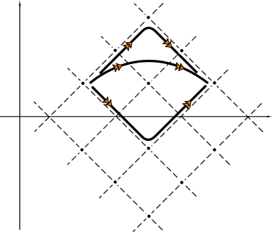
Figure 11: Compressed multi-walls in the maximal topological sector. a) Two level-$1$ compressed walls forming a double wall are penetrable. b) A level-$2$ compressed wall and a single wall forming a double wall are penetrable.

We summarize moduli matrices for all topological sectors in this model in Table 2.

Table 2: Topological sectors in the case of $N_{\rm C}=2,\,N_{\rm F}=4$

top. sector	moduli matrix	dim.	objects
$\langle 12\rangle\leftarrow\langle 12\rangle$	$H_{0}{}_{\langle 12\rangle}$	0	vacuum $\langle 12\rangle$
$\langle 12\rangle\leftarrow\langle 13\rangle$	$H_{0}{}_{\langle 12\leftarrow 13\rangle}$	2	elementary wall $a_{2}$
$\langle 12\rangle\leftarrow\langle 14\rangle$	$H_{0}{}_{\langle 12\leftarrow 14\rangle}$	4	double wall $(a_{2},a_{3})\oplus$ compressed wall $a_{2}a_{3}$
$\langle 12\rangle\leftarrow\langle 23\rangle$	$H_{0}{}_{\langle 12\leftarrow 23\rangle}\oplus H_{0}{}_{\langle 12\leftarrow 32\rangle}$	4	double wall $(a_{2},a_{1})\oplus$ compressed wall $a_{1}a_{2}$
$\langle 12\rangle\leftarrow\langle 24\rangle$	$H_{0}{}_{\langle 12\leftarrow 24\rangle}\oplus H_{0}{}_{\langle 12\leftarrow 42\rangle}$	6	$(a_{2},a_{3},a_{1})\oplus(a_{2}a_{3},a_{1})\oplus(a_{1}a_{2},a_{3})\oplus a_{1}a_{2}a_{3}$
$\langle 12\rangle\leftarrow\langle 34\rangle$	$H_{0}{}_{\langle 12\leftarrow 34\rangle}$	8	$(a_{2},a_{1},a_{3},a_{2})\oplus(a_{2}a_{3},a_{1},a_{2})\oplus(a_{2}a_{3},a_{1}a_{2})$
	$\oplus H_{0}{}_{\langle 12\leftarrow 43\rangle}$		$\oplus(a_{1}a_{2},a_{3},a_{2})\oplus(a_{1}a_{2}a_{3},a_{2})$
$\langle 13\rangle\leftarrow\langle 13\rangle$	$H_{0}{}_{\langle 13\rangle}$	0	vacuum $\langle 13\rangle$
$\langle 13\rangle\leftarrow\langle 14\rangle$	$H_{0}{}_{\langle 13\leftarrow 14\rangle}$	2	elementary wall $a_{3}$
$\langle 13\rangle\leftarrow\langle 23\rangle$	$H_{0}{}_{\langle 13\leftarrow 23\rangle}$	2	elementary wall $a_{1}$
$\langle 13\rangle\leftarrow\langle 24\rangle$	$H_{0}{}_{\langle 13\leftarrow 24\rangle}$	4	penetrable double wall $(a_{1},a_{3})$
$\langle 13\rangle\leftarrow\langle 34\rangle$	$H_{0}{}_{\langle 13\leftarrow 34\rangle}\oplus H_{0}{}_{\langle 13\leftarrow 43\rangle}$	6	$(a_{3},a_{1},a_{2})\oplus(a_{1},a_{2}a_{3})\oplus(a_{3},a_{1}a_{2})\oplus a_{1}a_{2}a_{3}$
$\langle 14\rangle\leftarrow\langle 14\rangle$	$H_{0}{}_{\langle 14\rangle}$	0	vacuum $\langle 14\rangle$
$\langle 14\rangle\leftarrow\langle 23\rangle$	-	-	(non-BPS state)
$\langle 14\rangle\leftarrow\langle 24\rangle$	$H_{0}{}_{\langle 14\leftarrow 24\rangle}$	2	elementary wall $a_{1}$
$\langle 14\rangle\leftarrow\langle 34\rangle$	$H_{0}{}_{\langle 14\leftarrow 34\rangle}$	4	double wall $(a_{1},a_{2})\oplus$ compressed wall $a_{1}a_{2}$
$\langle 23\rangle\leftarrow\langle 23\rangle$	$H_{0}{}_{\langle 23\rangle}$	0	vacuum $\langle 23\rangle$
$\langle 23\rangle\leftarrow\langle 24\rangle$	$H_{0}{}_{\langle 23\leftarrow 24\rangle}$	2	elementary wall $a_{3}$
$\langle 23\rangle\leftarrow\langle 34\rangle$	$H_{0}{}_{\langle 23\leftarrow 34\rangle}\oplus H_{0}{}_{\langle 23\leftarrow 43\rangle}$	4	double wall $(a_{3},a_{2})\oplus$ compressed wall $a_{2}a_{3}$
$\langle 24\rangle\leftarrow\langle 24\rangle$	$H_{0}{}_{\langle 24\rangle}$	0	vacuum $\langle 24\rangle$
$\langle 24\rangle\leftarrow\langle 34\rangle$	$H_{0}{}_{\langle 24\leftarrow 34\rangle}$	2	elementary wall $a_{2}$
$\langle 34\rangle\leftarrow\langle 34\rangle$	$H_{0}{}_{\langle 34\rangle}$	0	vacuum $\langle 34\rangle$

We now explain that the most of moduli parameters in the matrix (4.124) can be understood as Nambu-Goldstone modes except one moduli which is a quasi-Nambu-Goldstone mode. Let us concentrate on imaginary parts of moduli parameters in this moduli matrix. As described in Sec. 3.5, $(N_{\rm C}-1)(\tilde{N}_{\rm C}-1)$ quasi-Nambu-Goldstone parameters are contained in such parameters, while others are the Nambu-Goldstone parameters corresponding to broken global symmetry $U(1)^{N_{\rm F}-1}$. The case of $N_{\rm C}=2,N_{\rm F}=4$ is the simplest case containing quasi-Nambu-Goldstone parameters. We have only one quasi-Nambu-Goldstone mode: $(N_{\rm C}-1)(\tilde{N}_{\rm C}-1)=1$. Let us consider the global transformation of $U(1)^{N_{\rm F}-1}$,

$$H^{1} \!\rightarrow\! (H^{1})^{\prime}=H^{1}e^{i\Lambda},\ \Lambda={\rm diag.}(\lambda_{1},\lambda_{2},\lambda_{3},\lambda_{4}),\quad$$ (4.125)

with $\sum_{i=1}^{4}\lambda_{i}=0$. The operators for the elementary walls transform under this transformation as

$$a_{i}(r)\rightarrow(a_{i}(r))^{\prime}=e^{-i\Lambda}a_{i}(r)e^{i\Lambda}=e^{-i(\lambda_{i}-\lambda_{i+1})}a_{i}(r)=a_{i}(r^{\prime}),$$ (4.126)

and we find the complex moduli parameters $r_{i}$ to transform

$$r_{1} \rightarrow r_{1}^{\prime}=r_{1}-i(\lambda_{2}-\lambda_{3}),$$

$$r_{2} \rightarrow r_{2}^{\prime}=r_{2}-i(\lambda_{3}-\lambda_{4}),$$

$$r_{3} \rightarrow r_{3}^{\prime}=r_{3}-i(\lambda_{1}-\lambda_{2}),$$

$$r_{4} \rightarrow r_{4}^{\prime}=r_{4}-i(\lambda_{2}-\lambda_{3}).$$ (4.127)

Thus we find the solution in this $N_{\rm C}=2,\,N_{\rm F}=4$ case contains one quasi-Nambu-Goldstone parameter ${\rm Im}(r_{1}-r_{4})$.

5 Moduli Space for Non-Abelian Walls

In the first subsection, the moduli space for non-Abelian domain walls is shown to be homeomorphic to the complex Grassmann manifold. In the second subsection, we construct the moduli metric and show that it is a deformed Grassmann manifold.

5.1 Topology of the Wall Moduli Space

In this subsection we discuss the moduli space for non-Abelian domain walls. The $U(N_{\rm C})$ SUSY gauge theory with $N_{\rm F}$ hypermultiplets maximally admits $N_{\rm wall}$ parallel domain walls, with $N_{\rm wall}$ given in Eq. (3.69). All possible solutions can be constructed once the moduli matrix $H_{0}$ is given. The moduli matrix $H_{0}$ has a redundancy expressed as the world-volume symmetry (3.6) : $H_{0}\sim VH_{0}$ with $V\in GL(N_{\rm C},{\bf C})$. We thus find that the moduli space denoted by ${\cal M}_{N_{\rm F},N_{\rm C}}$ is homeomorphic to the complex Grassmann manifold:

$${\cal M}_{N_{\rm F},N_{\rm C}}\simeq\{H_{0}|H_{0}\sim VH_{0},V\in GL(N_{\rm C},{\bf C})\}\simeq G_{N_{\rm F},N_{\rm C}}\simeq{SU(N_{\rm F})\over SU(N_{\rm C})\times SU(\tilde{N}_{\rm C})\times U(1)}\,.$$ (5.1)

This is a compact (closed) set. On the other hand, for instance, scattering of two Abelian walls is described by a nonlinear sigma model on a non-compact moduli space [25, 26, 14]. We also find similar non-compact moduli such as relative distances and quasi-Nambu-Goldstone modes of orientational moduli in Sec. 3.5, and by an explicit analysis of multiple non-Abelian walls in Sec. 4. This fact of the compact moduli space consisting of non-compact moduli parameters can be consistently understood, if we note that the moduli space ${\cal M}_{N_{\rm F},N_{\rm C}}$ includes all BPS topological sectors (3.54) determined by the different boundary conditions. It is decomposed into

$${\cal M}_{N_{\rm F},N_{\rm C}}=\sum_{\rm BPS}{\cal M}^{\langle A_{1}A_{2}\cdots A_{N_{\rm C}}\rangle\leftarrow\langle B_{1}B_{2}\cdots B_{N_{\rm C}}\rangle}_{N_{\rm F},N_{\rm C}},\;$$ (5.2)

where the sum is taken over the BPS sectors. Note that it also includes the vacuum states with no walls $\langle A_{1}A_{2}\cdots A_{N_{\rm C}}\rangle\leftarrow\langle A_{1}A_{2}\cdots A_{N_{\rm C}}\rangle$ which correspond to $N_{\rm F}!/N_{\rm C}!\tilde{N}_{\rm C}!$ points on the moduli space. Although each sector (except for vacuum states) is in general not a closed set, the total space is compact. We call ${\cal M}_{N_{\rm F},N_{\rm C}}$ as the “total moduli space”. It is useful to rewrite this as a sum over the number of walls:

$${\cal M}_{N_{\rm F},N_{\rm C}}=\sum_{k=0}^{N_{\rm C}\tilde{N}_{\rm C}}{\cal M}_{N_{\rm F},N_{\rm C}}^{k}={\cal M}_{N_{\rm F},N_{\rm C}}^{0}\oplus{\cal M}_{N_{\rm F},N_{\rm C}}^{1}\oplus\cdots\oplus{\cal M}_{N_{\rm F},N_{\rm C}}^{N_{\rm C}\tilde{N}_{\rm C}}\,,$$ (5.3)

with ${\cal M}_{N_{\rm F},N_{\rm C}}^{k}$ the sum of the topological sectors with $k$-walls. Since the maximal number of walls is $N_{\rm C}\tilde{N}_{\rm C}$, ${\cal M}_{N_{\rm F},N_{\rm C}}^{N_{\rm C}\tilde{N}_{\rm C}}$ is identical to the maximal topological sector.

This decomposition can be understood as follows. Consider a $k$-wall solution and imagine a situation such that one of the outer-most walls goes to spatial infinity. We will obtain a ($k-1$)-wall configuration in this limit. This implies that the $k$-wall sector in the moduli space is an open set compactified by the moduli space of ($k-1$)-wall sectors on its boundary. Continuing this procedure we will obtain a single wall configuration. Pulling it out to infinity we obtain a vacuum state in the end. A vacuum corresponds to a point as a boundary of a single wall sector in the moduli space. The $k=0$ sector comprises a set of $N_{\rm F}!/N_{\rm C}!\tilde{N}_{\rm C}!$ points and does not have any boundary. Summing up all sectors, we thus obtain the total moduli space ${\cal M}_{N_{\rm F},N_{\rm C}}$ as a compact manifold. Note again that we include zero-wall sector, vacua without any walls.

These procedures are understood as a compactification in the mathematical theory of the moduli space. In the following we will see these in some simple examples.

1) Let us discuss the simplest example of $N_{\rm C}=1$ and $N_{\rm F}=2$. In the strong coupling limit $g\to\infty$ this model reduces to the massive HK nonlinear sigma model on $T^{*}{\bf C}P^{1}$ or the Eguchi-Hanson space (see Fig. 2). This model contains two vacua, $N$ and $S$ corresponding to the moduli matrices $H_{0}=(1,0)$ and $H_{0}=(0,1)$, respectively. Thus ${\cal M}_{2,1}^{k=0}\simeq N\oplus S$. It admits a single wall connecting them, corresponding to the moduli matrix $H_{0}=(1,e^{r})$ with $e^{r}\in{\bf C}-\{0\}$. This single wall possesses two real moduli parameters corresponding to a translational zero mode ${\rm Re}(r)$ and a zero mode ${\rm Im}(r)(\sim{\rm Im}(r)+2\pi n,\,n\in{\bf Z})$ arising from spontaneously broken internal $U(1)$ symmetry. So the moduli space for the one wall solution is homeomorphic to a cylinder without boundary: ${\cal M}_{2,1}^{k=1}\simeq{\bf R}\times S^{1}$. By taking a limit ${\rm Re}(r)\to-\infty$, the moduli matrix approaches to the vacuum $N$: $H_{0}\to(1,0)$. On the other hand, in the opposite limit ${\rm Re}(r)\to+\infty$, it approaches to the other vacuum $S$ as $H_{0}=(1,e^{r})\sim(e^{-r},1)\to(0,1)$, where we have multiplied $e^{-r}$ using the world-volume symmetry (3.6). Thus, adding two points $N$ and $S$ in ${\cal M}_{2,1}^{k=0}$ to two infinities of ${\cal M}_{2,1}^{k=1}$, we find that the total moduli space is homeomorphic to a sphere (see Fig. 12)

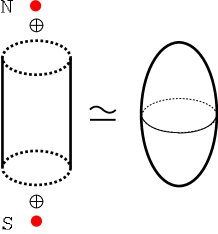
Figure 12: The total moduli space in the case of $N_{\rm F}=2$, $N_{\rm C}=1$. It is homeomorphic to a sphere, but its shape looks like a sausage when it is endowed with the metric.

$${\cal M}_{2,1}={\cal M}_{2,1}^{k=0}\oplus{\cal M}_{2,1}^{k=1}\simeq\{N\oplus S\}\oplus\{{\bf R}\times S^{1}\}\simeq S^{2}\simeq{\bf C}P^{1}\,.$$ (5.4)

This procedure of adding infinities is a two-point compactification in the mathematical moduli theory. Physically this corresponds to the following situation: Moving a wall to two spatial infinities, the configuration approaches to two vacuum states of this theory.

The moduli metric on this ${\bf C}P^{1}$ manifold is of course not the round Fubini-Study metric. It is deformed to break two isometries in $SU(2)$ preserving one $U(1)$ isometry. Therefore it locally looks like a sausage but the distance to the infinities diverges. We will return to this point in the end of this section but let us now make a comment on physical validity to consider the topology of the total moduli space instead of each topological sector. The authors in Ref. [43] constructed a solution of 1/4 BPS equation in a $D=4$, ${\cal N}=2$ SUSY theory. It is a composite soliton made of a wall and vortices (strings) ending on it. Topological stability of this composite soliton can be understood by interpreting vortices as sigma model lumps in the effective theory on the wall if and only if we consider the total moduli space (5.4) as the target space instead of the one-wall topological sector ${\cal M}_{2,1}^{k=1}\simeq{\bf R}\times S^{1}$. This is because the second homotopy group $\pi_{2}$ ensuring the topological stability of lumps is ${\bf Z}$ for ${\bf C}P^{1}$ but is trivial for ${\bf R}\times S^{1}$. The total moduli space (5.1) for general $N_{\rm F}$ and/or $N_{\rm C}$ provides the topological stability of more complicated composite solitons recently constructed by the present authors [44].

2) Next let us consider the case of $N_{\rm C}=1$ and $N_{\rm F}=3$. In the strong coupling limit $g\to\infty$ the model becomes the nonlinear sigma model on $T^{*}{\bf C}P^{2}$ homeomorphic to $T^{*}G_{3,2}$, the strong coupling limit of $N_{\rm C}=2$ and $N_{\rm F}=3$ discussed in Sec. 4.1. This model admits a double wall solution as the maximal topological sector. We will show that moduli space is homeomorphic to ${\bf C}P^{2}$. To this end it is useful to introduce a toric diagram. The toric diagrams for ${\bf C}P^{1}$ and ${\bf C}P^{2}$ are displayed in Fig. 13 .

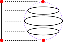
Figure 13: Toric diagrams. a) The toric diagram for ${\bf C}P^{1}$. ${\bf C}P^{1}$ admits one holomorphic $U(1)$ isometry as commuting $U(1)$ isometries. Dividing ${\bf C}P^{1}$ by this $U(1)$, we obtain the toric diagram for ${\bf C}P^{1}$ as a segment (1-simplex). It is parametrized by one $U(1)$ invariant which is the momentum map for the $U(1)$ action. ${\bf C}P^{1}$ is parametrized as a circle fibration over it. The circle shrinks at the endpoints of the segment. b) The toric diagram for ${\bf C}P^{2}$. The ${\bf C}P^{2}$ admits two commuting holomorphic $U(1)$ isometries. Dividing ${\bf C}P^{2}$ by $U(1)^{2}$ we obtain a toric diagram for ${\bf C}P^{2}$. It is parametrized by two $U(1)^{2}$ invariants which are the momentum maps for the $U(1)^{2}$ action. It consists of one triangle (2-simplex) without boundary, three open lines $A$-$B$, $B$-$C$ and $C$-$A$ on its edge and three points denoted by $A$, $B$ and $C$. ${\bf C}P^{2}$ is parametrized as a torus fibration over this toric diagram, and one cycle shrinks on three edge lines and both cycles shrink at three points $A$, $B$ and $C$. Three edges with circle fibers are ${\bf C}P^{1}$ submanifolds of ${\bf C}P^{2}$.

1. This model contains three discrete vacua at $A$, $B$ and $C$ corresponding to the moduli matrices $H_{0}=(0,0,1)$, $(0,1,0)$ and $(1,0,0)$, respectively. Therefore we have ${\cal M}_{3,1}^{k=0}=A\oplus B\oplus C$.

2. There exist two elementary walls interpolating between $A$ and $B$ and between $B$ and $C$ corresponding to the moduli matrices $H_{0}=(0,1,e^{s})$ and $(1,e^{r},0)$ ($e^{r},e^{s}\in{\bf C}-\{0\}\simeq{\bf R}\times S^{1}$), respectively. They approach to vacua as was seen above. A wall connecting $A$ and $C$ given by $H_{0}=(1,0,e^{s})$ is a compressed wall obtained from a double wall solution in a particular limit by compressing two walls without changing the topological sector or the wall tension, and so it is not included in ${\cal M}_{3,1}^{k=1}$. Therefore we have ${\cal M}_{3,1}^{k=1}\simeq{\bf R}\times S^{1}\oplus{\bf R}\times S^{1}$.

3. The moduli subspace for the double wall solution is generated by $H_{0}=(1,e^{r},e^{s})$ ($e^{r}\in{\bf C}$, $e^{s}\in{\bf C}-\{0\}$). It has a topology of ${\bf R}\times S^{1}\times{\bf C}$. It sweeps inside the triangle in Fig. 13-b) with the boundary line connecting $A$ and $C$ and without the both lines $A$-$B$ and $B$-$C$ (because they are elementary wall solutions ) and without three points $A$, $B$ and $C$. The torus fiber $({\rm Im}(r),{\rm Im}(s))\in T^{2}$ shrinks to ${\rm Im}(s)\in S^{1}$ at the line $A$-$C$ (${\rm Re}\,(r)\to-\infty$). Such a shrinking cycle ${\rm Im}(r)\in S^{1}$ with a moduli for distance ${\rm Re}(r)$ between two walls constitute $r\in{\bf C}$. The non-shrinking cycle ${\rm Im}(s)$ with center of mass position ${\rm Re}(s)$ comprise ${\bf R}\times S^{1}$. Therefore the moduli subspace for two walls is homeomorphic to ${\cal M}_{3,1}^{k=2}\simeq{\bf R}\times S^{1}\times{\bf C}$ (see Fig. 14).

   

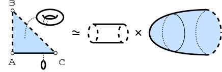
   Figure 14: The moduli subspace for the double wall configuration. It is homeomorphic to ${\bf R}\times S^{1}\times D$ with $D$ a two-dimensional disc without a boundary. The disc $D$ is endowed with the metric looking like a cigar.

   The factor ${\bf C}$ is homeomorphic to a disc $D$ without boundary. As found in [25, 26] $D$ is endowed with the metric looking like a cigar as shown in Fig. 14. It is also homeomorphic to the two dimensional Euclidean black hole metric. In this case, the metric for finite gauge coupling was also calculated exactly in [14] for particular values of $g$. The metric has the same topology, but is slightly deformed by $g$.

Combining all of these, we obtain ${\bf C}P^{2}$. We thus have found that the total moduli space is homeomorphic to ${\bf C}P^{2}$ (see Fig. 15):

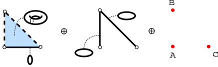
Figure 15: The sum ${\cal M}_{3,1}^{2}\oplus{\cal M}_{3,1}^{1}\oplus{\cal M}_{3,1}^{0}$. The double-wall and single-wall sectors are non-compact and the zero-wall (vacuum) sector is compact. The total space is ${\bf C}P^{2}$ in Fig. 13-b).

$${\cal M}_{3,1}={\cal M}_{3,1}^{k=0}\oplus{\cal M}_{3,1}^{k=1}\oplus{\cal M}_{3,1}^{k=2}$$

$$\hskip 28.45274pt\simeq\{A\oplus B\oplus C\}\oplus\{{\bf R}\times S^{1}\oplus{\bf R}\times S^{1}\}\oplus\{{\bf R}\times S^{1}\times D\}\simeq{\bf C}P^{2}\,.$$ (5.5)

The topological sectors ${\cal M}_{3,1}^{k=1}$ and ${\cal M}_{3,1}^{k=2}$ are open sets containing non-compact moduli parameters.

3) In the case of $N_{\rm C}=1$ and an arbitrary $N_{\rm F}$, the model reduces in the strong coupling limit to a nonlinear sigma model on $T^{*}{\bf C}P^{N_{\rm F}-1}$. In the same way we can write down a toric diagram parametrized by $N_{\rm F}-1$ invariants. The maximal number of walls is $N_{\rm F}-1$ and the ($N_{\rm F}-1$)-wall solutions given by the moduli matrix $H_{0}=(1,e^{r_{1}},\cdots,e^{r_{N_{\rm F}-1}})$ ($e^{r_{1}},\cdots,e^{r_{N_{\rm F}-2}}\in{\bf C}$, $e^{r_{N_{\rm F}-1}}\in{\bf C}-\{0\}$) sweep a ($N_{\rm F}-1$)-simplex of the maximal topological sector ${\cal M}_{N_{\rm F},1}^{k=N_{\rm F}-1}$ to which the $N_{\rm F}-1$ wall sector is homeomorphic. These parametrize almost all regions of ${\bf C}P^{N_{\rm F}-1}$ except for infinities (and so it is open). It is compactified by topological sectors with less numbers of walls by taking some limits.

1. If we take a limit ${\rm Re}\ (r_{I})\to-\infty$ for $1\leq I\leq N_{\rm F}-2$, the configuration remains in the maximal topological sector ${\cal M}_{N_{\rm F},1}^{N_{\rm F}-1}$, namely it does not give independent sectors.

2. On the other hand, in the limit of ${\rm Re}(r_{N_{\rm F}-1})\to-\infty$, we obtain $H_{0}=(1,e^{r_{1}},\cdots,e^{r_{N_{\rm F}-2}},0)$ in a different topological sector with walls less by one, ${\cal M}_{N_{\rm F},1}^{N_{\rm F}-2}$. Similarly in the limit of ${\rm Re}\,r_{N_{\rm F}-1}\to+\infty$ with keeping $r_{I}^{\prime}\equiv r_{I+1}-r_{1}$ ($1\leq I\leq N_{\rm F}-2$) finite and ${\rm Re}\,r_{1}\to\infty$, we obtain $H_{0}=(0,1,e^{r_{1}^{\prime}},\cdots,e^{r_{N_{\rm F}-2}^{\prime}})$ resulting again in ${\cal M}_{N_{\rm F},1}^{N_{\rm F}-2}$. Both sets of parameters parametrize almost all regions of ${\bf C}P^{N_{\rm F}-2}$’s except for infinities again.

The procedure 1. does not change topological sectors but 2. does. Continuing these two procedures 1. and 2. we reach at single walls. There exist ${}_{N_{\rm F}}C_{2}=\frac{1}{2}N_{\rm F}(N_{\rm F}-1)$ single wall solutions given by $H_{0}=(0,\cdots,0,1,0,\cdots,0,e^{r},0,\cdots,0)$ which correspond to one simplexes or ${\bf C}P^{1}$’s without two points. Among them, elementary walls in ${\cal M}_{N_{\rm F},1}^{1}$ are obtained as those given by the ($N_{\rm F}-1$) moduli matrices $H_{0}=(0,\cdots,0,1,e^{r},0,\cdots,0)$ with a pair of adjacent non-vanishing elements. The rest are subspaces in ${\cal M}_{N_{\rm F},1}^{k\geq 2}$. By adding $N_{\rm F}$ vacua $H_{0}=(0,\cdots,1,\cdots,0)$ as points in ${\cal M}_{N_{\rm F},1}^{0}$ further, we obtain the full moduli space as ${\bf C}P^{N_{\rm F}-1}$.

In the above discussion, we did not use the fact that we took the $g\to\infty$ limit, so this is true for finite $g$ (although the metric is deformed in general).

4) In more general cases, the strong coupling limit is the sigma model on $T^{*}G_{N_{\rm F},N_{\rm C}}$, which is not toric anymore. We do not have toric diagrams. However it is now obvious that all informations for the topology of the total moduli space is encoded into $H_{0}$. We thus have found that the total moduli space is homeomorphic to the complex Grassmann manifold, ${\cal M}_{N_{\rm F},N_{\rm C}}\simeq G_{N_{\rm F},N_{\rm C}}$, but the metric on it is not a homogeneous one. We construct the moduli metric in the next subsection.

It is interesting to observe that in our decomposition of the moduli space (5.3), the one wall sector ${\cal M}^{1}_{N_{\rm F},N_{\rm C}}$ includes elementary walls only, i.e. single walls that are not compressed walls. Compressed walls are contained in double- or multi-wall configurations as limits without changing boundary conditions. Therefore we can classify single walls into elementary or (non-elementary) compressed walls in terms of moduli space: moduli subspace for non-elementary walls belong to boundaries of moduli space of double or multi-walls, $\partial{\cal M}^{k\geq 2}_{N_{\rm F},N_{\rm C}}$, but elementary walls do not.

5.2 Metric on the Wall Moduli Space and Effective Field Theory

Effective theory on walls describes local fluctuations of moduli parameters depending on the world-volume coordinates $x^{\mu}$ ($\mu=0,\cdots,3$) and the Grassmann coordinates $\theta,\bar{\theta}$ in the $D=4$, ${\cal N}=1$ superspace (with four supercharges).

First we construct the effective action explicitly for the infinite gauge coupling limit $g\to\infty$. Following the Manton’s method [48] we promote moduli parameters in the moduli matrix $H_{0}$ to weakly varying fluctuating fields depending on the world-volume coordinates of walls. We deal with bosonic fluctuation described by complex scalars $\phi^{X}(x^{\mu})$ with $X=1,\cdots,N_{\rm C}\tilde{N}_{\rm C}$ for a while and then will promote them to chiral superfields later. Then $H^{1}$ and $H^{2}$ are given by

$$H^{1}(\phi,\phi^{*},y)=S^{-1}(\phi,\phi^{*},y)H_{0}(\phi)e^{My},\quad H^{2}=0\,.$$ (5.6)

Using the constraints (3.72) and (3.74) with $H^{2}=0$,

$$H^{1}H^{1}{}^{\dagger}=c{\bf 1}_{N_{\rm C}},\quad W_{\mu}=ic^{-1}(\partial_{\mu}H^{1})H^{1}{}^{\dagger},$$ (5.7)

the kinetic term in (3.75) reduces to

$${\cal L}_{\rm kin}={\rm Tr}\left({\cal D}_{\mu}H^{1}{}^{\dagger}{\cal D}^{\mu}H^{1}\right)={\rm Tr}\left(\partial_{\mu}H^{1}{}^{\dagger}\partial^{\mu}H^{1}({\bf 1}_{N_{\rm F}}-c^{-1}H^{1}{}^{\dagger}H^{1})\right).$$ (5.8)

Substituting (5.6) into this and using (3.71), we obtain the $y$-integrand of the effective Lagrangian

$${\cal L}_{\rm kin}=c\,\partial_{X}\partial_{X}^{*}\left({\rm Tr}\left[\log\Omega\right]\right)\partial_{\mu}\phi^{X}\partial^{\mu}\phi^{*X},$$ (5.9)

which is a Kähler nonlinear sigma model with the Kähler potential

$$K(\phi,\phi^{*},y)\equiv c{\rm Tr}\left[\log\Omega(\phi,\phi^{*},y)\right]=c\log\det\left[\Omega(\phi,\phi^{*},y)\right]\,.$$ (5.10)

Promoting bosonic fields $\phi^{X}$ to $D=4$, ${\cal N}=1$ chiral superfields $\phi^{X}(x,\theta,\bar{\theta})$ we obtain the effective Lagrangian for (multi) domain walls describing dynamics of moduli including fermionic superpartners as

$${\cal L}_{\rm walls}^{g\to\infty}=c\int d^{4}\theta\int dy\ \log\det\Omega_{g\to\infty}=c\int d^{4}\theta\int dy\ \log\det(H_{0}e^{2My}H_{0}{}^{\dagger})\;.$$ (5.11)

Note that this Lagrangian is invariant under a transformation of $H_{0}$

$$H_{0}\to H_{0}{}^{\prime}=e^{\Lambda}H_{0}\;$$ (5.12)

with an arbitrary $N_{\rm C}\times N_{\rm C}$ matrix of $D=4$, ${\cal N}=1$ chiral superfield $\Lambda(x,\theta,\bar{\theta})$. The Kähler potential receives a Kähler transformation

$$\log\det\Omega\to\log\det\Omega+\log\det\Lambda+\log\det\Lambda^{\dagger}$$ (5.13)

where the last two terms $\log\det\Lambda$ and $\log\det\Lambda^{\dagger}$ disappear under the $\theta$ integration in the Lagrangian (5.11). The transformation (5.12) is a local $U(N_{\rm C})$ gauge symmetry on the world volume of walls, although corresponding vector multiplet does not appear explicitly. It is actually enhanced to its complexification $U(N_{\rm C})^{\bf C}=GL(N_{\rm C},{\bf C})$ because the lowest component of $\Lambda$ are complex, and can be understood as a local symmetry originated from the global world-volume symmetry (3.6).

If the hypermultiplet masses are non-degenerate $M=0$, the integrand in the Lagrangian (5.11) is the Kähler potential for the Grassmann manifold with the maximal isometry $SU(N_{\rm F})$ acting on $H_{0}$ as $H_{0}\to H_{0}U$ with $U\in SU(N_{\rm F})$ [49]. In contrast, $SU(N_{\rm F})$ is explicitly broken down to $U(1)^{N_{\rm F}-1}$ by hypermultiplet masses $M$ for our non-degenerate mass case. Therefore the moduli space metric for non-Abelian domain walls is the deformed Grassmann manifold.

We have constructed the effective action on walls by the Manton’s method. Here we discuss a symmetry approach to the low-energy effective action in the spirit of the chiral Lagrangian in QCD. Since we use only symmetry to construct the action in this method, it determines the effective action only up to an ambiguity in the Kähler potential with an arbitrary function of invariants. The symmetry approach has an advantage of wide applicability, including the case of quantum corrections preserving the symmetry. In order to extract the true collective coordinates from the moduli matrix $H_{0}$ promoted to a matrix chiral superfield $H_{0}(x,\theta,\bar{\theta})$, we have to take account of the redundancy expressed by the world-volume symmetry (3.6). Since the moduli are promoted to fields on the world volume, it is most convenient to promote the world-volume symmetry $GL(N_{\rm C},{\bf C})$ into a local gauge symmetry on the world volume. One should note that this local gauge symmetry is described by an $N_{\rm C}\times N_{\rm C}$ matrix vector superfield $V(x,\theta,\bar{\theta})$ without kinetic terms. Hence $V(x,\theta,\bar{\theta})$ is a Lagrange multiplier field just to express the redundancy of the matrix chiral superfield $H_{0}(x,\theta,\bar{\theta})$ at least in the classical level. Then the world-volume gauge symmetry acts as

$$H_{0}\to e^{\Lambda}H_{0}\;,\hskip 14.22636pte^{V}\to e^{-\Lambda^{\dagger}}e^{V}e^{-\Lambda},$$ (5.14)

with $\Lambda(x,\theta,\bar{\theta})$ defined in (5.12). This gauge symmetry is complexified to $GL(N_{\rm C},{\bf C})$ but we call this gauge symmetry $U(N_{\rm C})$ as usual. Since the expression in Eq. (5.1) merely means the topology, the world-volume theory does not possess $SU(N_{\rm F})$ global symmetry. Instead $SU(N_{\rm F})$ was explicitly broken down to $U(1)^{N_{\rm F}-1}$ by the hypermultiplet masses. In this respect we decompose $H_{0}$ as

$$H_{0}=(h_{1},h_{2},\cdots,h_{N_{\rm F}}),$$ (5.15)

with $h_{A}(x,\theta,\bar{\theta})$ ($A=1,\cdots,N_{\rm F}$) an $N_{\rm C}$-vector of chiral superfields. The world-volume theory is invariant under $U(N_{\rm C})_{\rm local}\times U(1)^{N_{\rm F}-1}$ in which $U(1)^{N_{\rm F}-1}$ acts on $h_{A}$ as $h_{A}\to e^{i\alpha_{A}}h_{A}$ with a constraint $\sum_{A}\alpha_{A}=0$. We define invariants under these symmetries by

$$X_{A}\equiv h_{A}{}^{\dagger}e^{V}h_{A}\;.$$ (5.16)

When we construct the invariant Kähler potential for the low-energy effective Lagrangian these invariants bring in an ambiguity which cannot be determined by symmetry alone and depends on the detail of the theory. Thus the effective Lagrangian on the wall can be written by using an undetermined function $f_{g}$ of invariants $X_{A}$ which depends on the gauge coupling $g$ in the original gauge theory:

$${\cal L}_{\rm wall}^{g}=\int d^{4}\theta[f_{g}(X_{1},\cdots,X_{N_{\rm F}})-C\,{\rm tr}\,V],$$ (5.17)

where $C$ is the FI parameter for the world-volume gauge theory. Eliminating $V$ by its algebraic equation of motion we obtain the effective theory in terms of independent fields. This procedure is the Kähler quotient. We conjecture that Manton’s effective Lagrangian (5.11) may be contained in (5.17) as a particular form of $f_{g}$, although we have not yet succeeded to demonstrate it explicitly.

The effective theory (5.11) or (5.17) on the world volume of walls includes all topological sectors. Which sector it describes depends completely on which point on moduli space one chooses as the background. As far as one analyzes the effective theory perturbatively, it describes the topological sector to which the background belongs. This is consistent with the fact that the geodesic distance diverges if one wants to reach other topological sectors.

Here we make a comment on the difference between effective Lagrangians for walls and other solitons. Other solitons admit D-brane pictures. Instantons can be interpreted for instance by the D0-D4 system. The instanton moduli space is obtained as an effective field theory on the D0-branes as found in [19]. Taking its T-dual along the D4-brane world-volume it becomes D1-branes ending on D3-branes. The effective theory on D1-branes gives the monopole moduli space [20]. Effective Lagrangian for non-Abelian vortices has recently been derived by Hanany and Tong [21] in the Hanany-Witten brane configuration where vortices are identified with D1-branes. In all the cases, the gauge group $U(k)$ of these effective theories come from gauge invariance on $k$ D-branes. In contrast to these cases, in our wall case, the gauge group $U(N_{\rm C})$ on the wall effective Lagrangian is identical to that of the original gauge theory not related with the number of walls. We have not yet found brane constructions appropriate for the non-Abelian walls.

Before closing this section, we make a comment on a possible interpretation of our moduli space as a special Lagrangian submanifold. In the massless limit, the moduli space of vacua (the Higgs branch of the gauge theory) denoted as ${\cal M}_{\rm vac}^{M=0}$ was the cotangent bundle over the complex Grassmann manifold, ${\cal M}_{\rm vac}^{M=0}\simeq T^{*}G_{N_{\rm F},N_{\rm C}}$ (3.76). By introducing hypermultiplet masses, most points on ${\cal M}_{\rm vac}^{M=0}$ are lifted leaving some discrete points as vacua. The moduli space ${\cal M}_{N_{\rm F},N_{\rm C}}$ for walls is shown to be homeomorphic to $G_{N_{\rm F},N_{\rm C}}$ which is a base manifold of ${\cal M}_{\rm vac}^{M=0}$. It is a special Lagrangian submanifold of $T^{*}G_{N_{\rm F},N_{\rm C}}$. We expect that moduli space for non-Abelian domain walls in SUSY gauge theory with general gauge group and general matter contents is homeomorphic to a special Lagrangian submanifold in the massless Higgs branch of vacua ${\cal M}_{\rm vac}^{M=0}$ of that gauge theory.

6 Discussion

Let us list some of the interesting topics for future researches.

As was shown in (5.11), the moduli space metric is deformed by hypermultiplet masses. We assumed that all masses are non-degenerate, so the global symmetry was $U(1)^{N_{\rm F}-1}$. We expect that this expression is valid even in the case that there exist mass degeneracy. However Eq. (5.11) can contain non-normalizable modes also. This is most easily exhibited for the case of $M=0$. In that case, the Kähler potential inside the $y$-integration is the standard one for the complex Grassmann manifold with the $SU(N_{\rm F})$ isometry. Is is a base manifold of the massless moduli space of vacua $T^{*}G_{N_{\rm F},N_{\rm C}}$. The integrand is independent of $y$ and hence the $y$-integration diverges. For partially degenerate masses we will obtain some non-Abelian localized zero modes also. To obtain effective theory on the world volume of walls, we have to throw away non-normalizable modes. Degenerate mass should also provides richer global symmetry [16], which is likely to have implications to localization of non-Abelian gauge bosons on walls. The case of degenerate masses is one of the most interesting and immediate future problem.

We have found previously for Abelian gauge theories that coupling the tensor multiplet provides the localized massless Abelian gauge boson on the wall [14]. We wish to come back to the problem of coupling tensor multiplets to the non-Abelian gauge theories admitting non-Abelian walls. We hope to localize non-Abelian gauge bosons on the non-Abelian walls with four-dimensional world volume by coupling the tensor multiplets appropriately.

We have discussed only the topological sector containing BPS multi-walls. However, our model contains the topological sectors admitting no BPS walls also. The number of the topological sectors admitting no BPS walls has been given in (3.65), which is one for $N_{\rm C}=2$ and $N_{\rm F}=4$ and five for $N_{\rm C}=2$ and $N_{\rm F}=5$ as seen in Fig. 16. For larger $N_{\rm C}$ or $N_{\rm F}$, our model contains many more topological sectors admitting no BPS walls. For instance in the case of $N_{\rm C}=2$ and $N_{\rm F}=4$, a wall configuration $\langle 23\rangle\leftarrow\langle 14\rangle$ is made by a BPS wall $\langle 13\rangle\leftarrow\langle 14\rangle$ and an anti-BPS wall $\langle 23\rangle\leftarrow\langle 13\rangle$, or by a BPS wall $\langle 13\rangle\leftarrow\langle 14\rangle$ and an anti-BPS wall $\langle 23\rangle\leftarrow\langle 24\rangle$. The BPS bound for this topological sector is never saturated by these configurations, irrespective of the bound taking positive, zero, or negative values. We do not know if the walls composing these configurations are interacting or not. If they are interacting it is very interesting to investigate whether they form a stable bound state of walls or not, as was found in a simpler model in four dimensions [51]. The fate of $U(1)$ zero modes is also interesting.

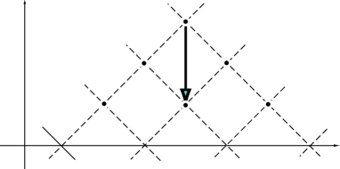
Figure 16: Non-BPS walls. a) $N_{\rm C}=2$ and $N_{\rm F}=4$. b) $N_{\rm C}=2$ and $N_{\rm F}=5$.

Even if non-BPS wall solutions are difficult to construct, we can construct the effective action by using the nonlinear realization method or the Green-Schwarz method, which has been worked out in four space-time dimensions [52].

Coupling with gravity has been discussed for single wall and multi-wall solutions in the case of Abelian gauge theories [53, 27]. In the limit of zero width of the wall, the BPS wall solution reduces to the Randall-Sundrum model. Therefore the Abelian wall embedded into supergravity can be regarded as a smooth regularization of the AdS space in the Randall-Sundrum model by finite wall width constructed by physical scalar fields. It has been found that the necessary gravitational deformations can have another parameter giving asymmetry of the bulk cosmological constant between left and right of the wall. To embed the globally SUSY nonlinear sigma model into supergravity, it has been difficult to obtain appropriate gravitational deformations of the target manifold. However, treating the model as a hyper-Kähler quotient using the gauge theory, it has been found to obtain the appropriate quaternionic manifold. It was essential to use the off-shell formalism [54] to couple the system to five-dimensional supergravity. Our formulation is a natural setting to embed the non-Abelian walls into the supergravity. We hope to complete the task in near future.

Moduli spaces for walls and vortices are Kähler whereas those for monopoles and instantons are hyper-Kähler. In [21] the vortex moduli space was shown to be a special Lagrangian submanifold of the ADHM instanton moduli space. Investigating our wall moduli space as some middle dimensional manifold of the monopole moduli space is an interesting future problem.

The moduli space for non-Abelian walls has turned out in this paper to be the complex Grassmann manifold. Taking a large $N_{\rm F}$ limit, $N_{\rm F}\to\infty$, it becomes the infinite dimensional Grassmann manifold. It is a famous fact that the moduli space of the KdV equation is the infinite dimensional Grassmann manifold. Therefore we suspect that there may be some deep connection between our model and integrable systems.

Appendix A Positions of Walls

In this Appendix we present the method to evaluate the positions of walls. With the infinite gauge coupling, det$\Omega$ can be calculated explicitly for a given moduli matrix $H_{0}$ as

$$\det(\,\Omega) = \det\left(\frac{1}{c}H_{0}e^{2My}H_{0}^{\dagger}\right)=\sum_{\langle A\rangle\in{\rm vacua}}\Big{|}{\rm det}\left(\frac{1}{c}H_{0}e^{My}H^{\dagger}_{0\langle A\rangle}\right)\Big{|}^{2}$$ (A.1)

$$= \sum_{\langle A\rangle\in{\rm vacua}}\Big{|}{\rm det}\left(\frac{1}{c}H_{0}H^{\dagger}_{0\langle A\rangle}\right)\Big{|}^{2}{\rm exp}\left({2\sum_{r=1}^{N_{\rm C}}m_{A_{r}}y}\right),$$

where sum is taken over the whole supersymmetric vacua labeled by $\langle A\rangle=\langle A_{1}A_{2}\cdots A_{r}\cdots A_{N_{\rm C}}\rangle$. Note that elements of the $N_{\rm C}\times N_{\rm C}$ matrix $H_{0}H^{\dagger}_{0\langle A\rangle}$ is given by $\left(H_{0}H^{\dagger}_{0\langle A\rangle}\right)^{r}{}_{s}=\sqrt{c}H_{0}^{rA_{s}}$. In vacua, the energy density vanishes $({c/2}){\partial_{y}^{2}}\log{\rm det}\Omega=0$ and the difference of $({c/2}){\partial_{y}}\log{\rm det}\Omega$ gives the topological charge of walls. We expect that det$\Omega$ exhibits a behaviour similar to the above formula (A.1) containing exponential factor of $\sum_{r=1}^{N_{\rm C}}m_{A_{r}}y$, even if we consider the case of finite gauge couplings.

By use of the form (A.1), we can guess positions of walls more accurately without calculating the energy density. For simplicity, let us consider the following $N_{\rm F}=3$ case,

$$\psi(y)\equiv\log{\rm det}\Omega = \log\left(e^{2f_{1}(y)}+e^{2f_{2}(y)}+e^{2f_{3}(y)}\right),$$

with linear functions $f_{i}(y)\equiv m_{i}y-u_{i},i=1,2,3$, and we assume $m_{1}>m_{2}>m_{3}$. Because of the exponential dependence in $y$, only one exponential factor in det$\Omega$ is dominant in each vacuum, thus $\psi(y)$ is close to the linear function of the dominant exponential

$$\psi(y)\simeq{\rm max}\left(f_{1}(y),\,f_{2}(y),\,f_{3}(y)\right).$$ (A.2)

As compared in Fig.17, the linear approximation (A.2) for $\psi(y)$ is accurate except near the transition region. Since $\partial_{y}^{2}\psi(y)$ gives the energy density of walls, position of walls are obtained as intersection points of the linear functions for each region defined by

$$y_{1} = {u_{1}-u_{2}\over m_{1}-m_{2}},\quad y_{2}={u_{2}-u_{3}\over m_{2}-m_{3}},\quad y_{12}={u_{1}-u_{3}\over m_{1}-m_{3}},$$ (A.3)

if the two linear functions are really dominant in that region of $y$. Note that if other linear functions are dominant, the intersection point is hidden by contributions from other terms and there is no wall at that point. Thus we observe that in the case $y_{1}>y_{2}$ there exist two walls whose positions are represented by $y_{1}$ and $y_{2}$, while in the case $y_{1}<y_{2}$ the configuration of walls looks approximately like one wall whose position is given by $y_{12}$. If we take the limit of $y_{2}\rightarrow\infty$ with $y_{12}$ fixed, we obtain a compressed wall located at $y_{12}$.

Figure 17: Comparison of the profile of $z=\psi(y),f_{1}(y),f_{2}(y),f_{3}(y)$ as functions of $y$. Linear functions $f_{i}$ are good approximations in their respective dominant regions.

Appendix B The Standard Form of $H_{0}^{1}$

In this Appendix, we show that any moduli matrix $H_{0}^{1}$ can be transformed to the standard form

$$H_{0}^{1}=\left(\begin{array}[]{c}\begin{picture}(380.0,90.0)(0.0,0.0)\put(10.0,-5.0){\scalebox{0.8}{\includegraphics{stand.eps}}} \end{picture}\begin{picture}(0.0,0.0)(-25.0,-37.0)\put(-400.0,-25.0){{\Huge$0$}} \put(-385.0,65.0){$A_{1}$} \put(-338.0,65.0){$A_{2}$} \put(-305.0,65.0){$\cdots$} \put(-248.0,65.0){$A_{N_{\rm C}}$} \put(-115.0,65.0){$B_{2}$} \put(-82.0,65.0){$B_{1}{\cdot}{\cdot}{\cdot}$} \put(-50.0,65.0){$B_{N_{\rm C}}$} \put(-385.0,39.0){1} \put(-338.0,39.0){0} \put(-275.0,39.0){0} \put(-338.0,21.0){1} \put(-260.0,2.0){0} \put(-248.0,-34.0){1} \put(0.0,-34.0){.} \put(-85.0,0.0){{\Huge$0$}} \end{picture}\end{array}\right)$$ (B.2)

Here, the matrix elements in gray color with flavor indices $A_{r}<A<B_{r}$ and in black color with flavor $B_{r}$ represent complex numbers which can and cannot vanish, respectively. Vanishing elements are fixed by the world-volume symmetry (3.6). We use the following simplified graphical representation

$$\begin{picture}(170.0,50.0)(-230.0,0.0)\put(-230.0,0.0){\scalebox{0.33333}{\includegraphics{def-mat1.eps}}} \put(-157.0,40.0){{\scriptsize 1}} \put(-133.0,31.0){{\scriptsize 1}} \put(-88.0,4.0){{\scriptsize 1}} \put(-170.0,20.0){$\equiv$} \end{picture},\qquad\begin{picture}(100.0,50.0)(0.0,0.0)\put(0.0,0.0){\scalebox{0.33333}{\includegraphics{def-mat2.eps}}} \put(30.0,20.0){$\equiv$} \end{picture}.$$ (B.3)

We now give a proof that an arbitrary moduli matrix $H_{0}^{1}$ can be brought to the standard form by the world-volume symmetry, and that no freedom of the world-volume symmetry remains once we have the standard form. Let us begin with arranging the left side of $H_{0}^{1}$. Let us assume that the first flavor index which has at least one non-vanishing element is $A_{1}$:

$$H_{0}^{1}=\left(\begin{array}[]{c}\begin{picture}(140.0,90.0)(0.0,0.0)\put(30.0,-5.0){\scalebox{0.3}{\includegraphics{h01--1.eps}}} \end{picture}\begin{picture}(0.0,0.0)(-65.0,-35.0)\put(-170.0,60.0){$A_{1}$} \put(-210.0,0.0){{\large$0$}} \end{picture}\end{array}\right),$$ (B.5)

In this equation, the right side of $H_{0}^{1}$ denoted by a wavy line indicates that the form on this side is not yet specified.

By using a part of degree of freedom of the world-volume symmetry $V\in GL(N_{\rm C},\mathbf{C})$ in (3.6), it is possible to transform the $A_{1}$-th column to $(1,0,\cdots,0)^{T}$. Then the matrix is of the form

$$H_{0}^{1}=\left(\begin{array}[]{c}\begin{picture}(190.0,80.0)(0.0,0.0)\put(20.0,-5.0){\scalebox{0.3}{\includegraphics{h01--2.eps}}} \end{picture}\begin{picture}(0.0,0.0)(-45.0,-30.0)\put(-165.0,55.0){$A_{2}$} \put(-209.0,55.0){$A_{1}$} \put(-206.0,35.0){1} \put(-230.0,-10.0){{\Huge$0$}} \end{picture}\end{array}\right),$$ (B.7)

where we have assumed that elements enclosed by the dashed line happen to vanish and that the region enclosed by the solid line in the $A_{2}$-th column has at least one non-zero element. The following world-volume symmetry (3.6) remains after the fixing of (B.7):

$$V=\left(\begin{array}[]{c}\begin{picture}(80.0,80.0)(0.0,0.0)\put(-3.0,-5.0){\scalebox{0.3}{\includegraphics{v--1.eps}}} \end{picture}\begin{picture}(0.0,0.0)(-30.0,-30.0)\put(-108.0,35.0){1} \put(-109.0,-10.0){{\large$0$}} \end{picture}\end{array}\right).$$ (B.9)

Repeating these fixings $N_{\rm C}$ times, $H_{0}^{1}$ can be transformed to an echelon form

$$H_{0}^{1}=\left(\begin{array}[]{c}\begin{picture}(250.0,80.0)(0.0,0.0)\put(10.0,-5.0){\scalebox{0.3}{\includegraphics{h01--3.eps}}} \end{picture}\begin{picture}(0.0,0.0)(-30.0,-32.0)\put(-224.0,55.0){$A_{2}$} \put(-267.0,55.0){$A_{1}$} \put(-144.0,55.0){$A_{N_{\rm C}}$} \put(-263.0,34.0){1} \put(-221.0,18.0){1} \put(-140.0,-30.0){1} \put(-260.0,-20.0){{\Huge$0$}} \end{picture}\end{array}\right).$$ (B.11)

Then the world-volume symmetry (B.9) reduces to

$$V=\left(\begin{array}[]{c}\begin{picture}(80.0,80.0)(0.0,0.0)\put(0.0,-5.0){\scalebox{0.3}{\includegraphics{v--2.eps}}} \end{picture}\begin{picture}(0.0,0.0)(-35.0,-30.0)\put(-108.0,36.0){1} \put(-92.0,20.0){1} \put(-44.0,-28.0){1} \put(-110.0,-20.0){{\Huge$0$}} \end{picture}\end{array}\right).$$ (B.13)

Next we fix the right side of $H_{0}^{1}$ by using the remaining world-volume symmetry (B.13). Let the first non-vanishing column from the right be the $B_{r}$-th flavor and its lowest non-vanishing component be in the $r$-th row, like

$$H_{0}^{1}=\left(\begin{array}[]{c}\begin{picture}(180.0,80.0)(0.0,0.0)\put(0.0,-5.0){\scalebox{0.3}{\includegraphics{h01--4.eps}}} \end{picture}\begin{picture}(0.0,0.0)(-50.0,-33.0)\put(-90.0,55.0){$B_{r}$} \put(-66.0,-29.0){{\Large$0$}} \put(-230.0,-20.0){{\Large$0$}} \put(-28.0,-10.0){$r$} \end{picture}\end{array}\right)\ \ \ .$$ (B.15)

It is possible to eliminate the region enclosed by the dashed line in (B.15) by using (B.13). Then $H_{0}^{1}$ and the world-volume symmetry become

$$H_{0}^{1}=\left(\begin{array}[]{c}\begin{picture}(165.0,90.0)(0.0,0.0)\put(0.0,0.0){\scalebox{0.3}{\includegraphics{h01--5.eps}}} \put(142.0,95.0){$B_{r}$} \put(10.0,20.0){{\Huge$0$}} \put(190.0,30.0){$r$} \end{picture}\end{array}\right)\ \ ,\quad V=\left(\begin{array}[]{c}\begin{picture}(80.0,90.0)(0.0,0.0)\put(-2.0,0.0){\scalebox{0.3}{\includegraphics{v--25.eps}}} \put(6.0,72.0){1} \put(39.0,40.0){1} \put(73.0,7.0){1} \put(5.0,15.0){{\Huge$0$}} \put(38.0,95.0){$r$} \put(105.0,40.0){$r$} \end{picture}\end{array}\right)\ \ \ ,$$ (B.18)

where elements enclosed by the dashed line in $H_{0}^{1}$ vanish accidentally and the $r$-th column in $V$ has been used for this fixing. By using elements enclosed by the dashed line in $V$ in Eq. (B.18), it is possible to eliminate the $(r,\ A_{r+1}),\ (r,\ A_{r+2}),\ \cdots,\ (r,\ A_{N_{\rm F}})$ elements in $H_{0}^{1}$. Then $H_{0}^{1}$ and remaining world-volume symmetry become

$$H_{0}^{1}=\left(\begin{array}[]{c}\begin{picture}(335.0,110.0)(0.0,0.0)\put(0.0,-30.0){\scalebox{0.41667}{\includegraphics{h01--6.eps}}} \put(60.0,120.0){$A_{r}$} \put(98.0,120.0){$A_{r+1}$} \put(140.0,120.0){$A_{r+2}\ \cdots$} \put(220.0,120.0){$A_{r+3}$} \put(305.0,120.0){$B_{r}$} \put(65.0,57.0){\small 1} \put(102.0,57.0){\footnotesize 0} \put(145.0,57.0){\footnotesize 0} \put(226.0,57.0){\footnotesize 0} \put(104.0,41.0){\footnotesize 1} \put(145.0,25.0){\footnotesize 1} \put(226.0,-8.0){\footnotesize 1} \put(29.0,15.0){{\Huge$0$}} \put(304.0,5.0){{\Huge$0$}} \put(365.0,57.0){$r$} \end{picture}\end{array}\right),\quad V=\left(\begin{array}[]{c}\begin{picture}(80.0,90.0)(0.0,0.0)\put(0.0,0.0){\scalebox{0.3}{\includegraphics{v--3.eps}}} \put(10.0,72.0){1} \put(43.0,40.0){1} \put(75.0,7.0){1} \put(9.0,7.0){{\Huge$0$}} \put(43.0,89.0){$r$} \put(101.0,40.0){$r$} \end{picture}\end{array}\right)\ \ ,$$ (B.21)

respectively.

Let us define $H_{0}^{1}[r]$ as the $(N_{\rm C}-1)\times N_{\rm F}$ submatrix removing the $r$-th row in the matrix $H_{0}$ and the $(N_{\rm C}-1)\times(N_{\rm C}-1)$ matrix $V[r]$ by removing the $r$-th row and the $r$-th column in the matrix $V$. Obviously, we can repeat the above procedure for $(H_{0}^{1}[r],V[r])$. Furthermore, the procedure to obtain $(H_{0}^{1}[r],V[r])$ from $(H_{0}^{1},V)$ can be repeated for $(H_{0}^{1}[r],V[r])$ to obtain $(H_{0}^{1}[r,s],V[r,s])$. Continuing this process $N_{\rm C}$ times, all degrees of freedom in $V$ are finally used to fix $H^{1}_{0}$ to the standard form (B.2).

Let us give an alternative procedure to find the standard form which is equivalent to the above procedure. This procedure should be more practical if one wishes to list up all matrices in the standard form parametrizing the given topological sector labeled by $\langle A_{1}A_{2}\cdots A_{N_{\rm C}}\rangle\leftarrow\langle B_{1}B_{2}\cdots B_{N_{\rm C}}\rangle$. Let us first list up all possible orderings of $B_{r}$. Once $A_{r}$ and $B_{r}$ are chosen, we can find the vanishing elements between $A_{r}$ and $B_{r}$ in the $r$-th row in the following way. Let us illustrate the method using an example of $N_{\rm C}=6$ with general $N_{\rm F}$:

$$H_{0}^{1}=\left(\begin{array}[]{c}\begin{picture}(385.0,90.0)(0.0,0.0)\put(0.0,-3.0){\scalebox{0.5}{\includegraphics{h01-ex.eps}}} \end{picture}\end{array}\right),\put(-410.0,60.0){$A_{1}$}\put(-380.0,60.0){$A_{2}$}\put(-345.0,60.0){$A_{3}$}\put(-310.0,60.0){$A_{4}$}\put(-277.0,60.0){$A_{5}$}\put(-237.0,60.0){$A_{6}$}\put(-200.0,60.0){$B_{5}$}\put(-152.0,60.0){$B_{2}$}\put(-107.0,60.0){$B_{4}$}\put(-91.0,60.0){$B_{6}$}\put(-75.0,60.0){$B_{1}$}\put(-45.0,60.0){$B_{3}$}\put(-400.0,-30.0){{\Huge$0$}}\put(-50.0,-30.0){{\Huge$0$}}\put(-408.0,40.0){\footnotesize 1}\put(-380.0,40.0){\footnotesize 0}\put(-310.0,40.0){\footnotesize 0}\put(-278.0,40.0){\footnotesize 0}\put(-237.0,40.0){\footnotesize 0}\put(-380.0,26.0){\footnotesize 1}\put(-278.0,26.0){\footnotesize 0}\put(-345.0,12.0){\footnotesize 1}\put(-310.0,12.0){\footnotesize 0}\put(-278.0,12.0){\footnotesize 0}\put(-237.0,12.0){\footnotesize 0}\put(-310.0,-2.0){\footnotesize 1}\put(-278.0,-2.0){\footnotesize 0}\put(-278.0,-16.0){\footnotesize 1}\put(-237.0,-32.0){\footnotesize 1}$$ (B.23)

1) Let $B_{r_{1}}$ the smallest among all the $B_{r}$. The $(A_{r_{1}},r_{1})$ element should be unity, according to the rule of constructing the standard form. Then all the elements above this $(A_{r_{1}},r_{1})$ element in the $A_{r_{1}}$-th column vanish. 2) Remove the $r_{1}$-th row and the $A_{r_{1}}$-th column from $H_{0}^{1}$. 3) Continue the same procedure $N_{\rm C}$ times. Then we obtain the standard form in Eq. (B.23).

The generic region of the topological sector is covered by the generic moduli matrix with the ordering $B_{1}<B_{2}<\cdots<B_{N_{\rm C}}$. On the other hand the subspace with the smallest dimension is covered by the moduli matrix with the ordering $B_{1}>B_{2}>\cdots>B_{N_{\rm C}}$ which has $\frac{1}{2}N_{\rm C}(N_{\rm C}-1)$ zero elements by fixing of $V$. The other orderings are of intermediate dimensions between these two moduli matrices.

Appendix C A Proof of $H_{0}^{2}=0$

In our wall configurations, $H^{1}$ is generated by the moduli matrix $H_{0}^{1}$, but $H^{2}$ always vanishes: $H_{0}^{2}=0$. In this Appendix we give a proof of $H_{0}^{2}=0$. In the case of non-degenerate hypermultiplet masses, this can be proved by requiring convergence of $H^{2}$ at $y\rightarrow\pm\infty$. The procedure of the proof is as follows. First, using finiteness of the solution $H^{1}=S^{-1}H_{0}^{1}e^{My}$ at $y\rightarrow\pm\infty$, we will estimate the order of divergence in $y\rightarrow\pm\infty$ for elements in the $N_{\rm C}\times N_{\rm C}$ matrix $S$ defined in Eq. (3.1). Then, we study conditions for elements of $H_{0}^{2}$ imposed by convergence of $H^{2}(=S^{\dagger}H_{0}^{2}e^{-My})$ at $y\rightarrow\pm\infty$. At this stage, most elements of $H_{0}^{2}$ are proved to vanish. The remaining elements in $H_{0}^{2}$ are also proved to vanish by the orthogonality condition for the moduli matrices $H_{0}^{1}$ and $H_{0}^{2}$: $H_{0}^{1}H_{0}^{2\dagger}=0$ (3.7).

First, let us investigate conditions for elements of $H_{0}^{2}$ imposed by convergence of $H^{2}=S^{\dagger}H_{0}^{2}e^{-My}$ at $y\rightarrow+\infty$. To this end, introduce the notation $\mathcal{O}_{A}^{\pm}$ which represents the order of $e^{\pm m_{A}|y|}$ at $y\rightarrow\infty$. By using the standard form of $H_{0}^{1}$, the order of the leading element in each row of $H_{0}^{1}e^{My}$ at $y\rightarrow+\infty$ is found to be

$$H_{0}^{1}e^{My}=\left(\begin{array}[]{c}\begin{picture}(180.0,90.0)(0.0,0.0)\put(0.0,0.0){\scalebox{0.3}{\includegraphics{h01emy.eps}}} \end{picture}\end{array}\right),\put(-207.0,55.0){$A_{1}$}\put(-167.0,55.0){$A_{2}$}\put(-88.0,55.0){$A_{N_{\rm C}}$}\put(-209.0,34.0){{\scriptsize$\mathcal{O}_{A_{1}}^{+}$}}\put(-167.0,18.0){{\scriptsize$\mathcal{O}_{A_{2}}^{+}$}}\put(-86.0,-31.0){{\scriptsize$\mathcal{O}_{A_{N_{\rm C}}}^{+}$}}\put(-210.0,-20.0){{\Huge$0$}}$$ (C.2)

where the order of divergence for subleading elements are less than the leading element in each row. Therefore, in order that $H^{1}$ converges at $y\rightarrow+\infty$, the orders of $S^{-1}$ and $S^{\dagger}$ should be

$$S^{-1}=\left(\begin{array}[]{c}\begin{picture}(80.0,90.0)(0.0,0.0)\put(0.0,0.0){\scalebox{0.3}{\includegraphics{s--1-1.eps}}} \put(9.0,74.0){{\scriptsize$\mathcal{O}_{A_{1}}^{-}$}} \put(25.0,58.0){{\scriptsize$\mathcal{O}_{A_{2}}^{-}$}} \put(73.0,10.0){{\scriptsize$\mathcal{O}_{A_{N_{\rm C}}}^{-}$}} \put(20.0,19.0){{\Huge$0$}} \end{picture}\end{array}\right)\ ,\ S^{\dagger}=\left(\begin{array}[]{c}\begin{picture}(80.0,90.0)(0.0,0.0)\put(-1.0,0.0){\scalebox{0.3}{\includegraphics{s--1-2.eps}}} \put(3.0,70.0){{\scriptsize$\mathcal{O}_{A_{1}}^{+}$}} \put(19.0,54.0){{\scriptsize$\mathcal{O}_{A_{2}}^{+}$}} \put(67.0,6.0){{\scriptsize$\mathcal{O}_{A_{N_{\rm C}}}^{+}$}} \put(60.0,50.0){{\Huge$0$}} \end{picture}\end{array}\right),$$ (C.5)

where we have used $U(N_{\rm C})$ gauge symmetry to fix $S^{-1}$ as the upper triangular matrix with real diagonal elements. Since the order of $H_{0}^{2}e^{-My}$ is

$$H_{0}^{2}e^{-My}=\left(\begin{array}[]{c}\begin{picture}(100.0,70.0)(0.0,0.0)\put(0.0,0.0){\scalebox{0.3}{\includegraphics{h02e-my.eps}}} \end{picture}\begin{picture}(0.0,0.0)(-30.0,-30.0)\put(-128.0,0.0){{\small$\mathcal{O}_{1}^{-}$}} \put(-105.0,0.0){{\small$\mathcal{O}_{2}^{-}$}} \put(-47.0,0.0){{\small$\mathcal{O}_{N_{\rm F}}^{-}$}} \end{picture}\end{array}\right),$$ (C.7)

the order of the first row of $H^{2}=S^{\dagger}H_{0}^{2}e^{-My}$ becomes

$$H^{2}\Bigl{|}_{\rm 1-st\ row}=(\mathcal{O}_{A_{1}}^{+}\mathcal{O}_{1}^{-},\ \mathcal{O}_{A_{1}}^{+}\mathcal{O}_{2}^{-},\ \cdots,\ \mathcal{O}_{A_{1}}^{+}\mathcal{O}_{N_{\rm F}}^{-}).$$ (C.8)

Therefore, convergence of $H^{2}$ at $y\rightarrow+\infty$ requires

$$H_{0}^{2}\Bigl{|}_{\rm 1-st\ row}=\left(\begin{array}[]{c}\begin{picture}(200.0,20.0)(0.0,0.0)\put(-1.0,0.0){\scalebox{0.3}{\includegraphics{h02-1st-row.eps}}} \end{picture}\begin{picture}(0.0,0.0)(-10.0,-3.0)\put(-162.0,20.0){ $A_{1}$} \put(-135.0,0.0){ $0\ \ \ \cdots\ \ \ \cdots\ \ \ 0$} \end{picture}\end{array}\right).$$ (C.10)

Similarly, the $r$-th row of $H_{0}^{2}$ is of the form

$$H_{0}^{2}\Bigl{|}_{\rm r-th\ row}=\left(\begin{array}[]{c}\begin{picture}(200.0,20.0)(0.0,0.0)\put(0.0,0.0){\scalebox{0.3}{\includegraphics{h02-r-th-row.eps}}} \end{picture}\begin{picture}(0.0,0.0)(-15.0,-3.0)\put(-133.0,20.0){ $A_{r}$} \put(-110.0,0.0){ $0\ \ \ \cdots\ \ \ \ 0$} \end{picture}\end{array}\right).$$ (C.12)

Then, convergence of $H^{2}$ at $y\rightarrow+\infty$ requires that $H_{0}^{2}$ is in the form of

$$H_{0}^{2}=\left(\begin{array}[]{c}\begin{picture}(180.0,80.0)(0.0,0.0)\put(0.0,-5.0){\scalebox{0.3}{\includegraphics{h02--1.eps}}} \end{picture}\begin{picture}(0.0,0.0)(-40.0,-35.0)\put(-90.0,15.0){{\Huge$0$}} \put(-177.0,55.0){$A_{1}$} \put(-145.0,55.0){$A_{2}\ \ \cdots$} \put(-53.0,55.0){$A_{N_{\rm C}}$} \end{picture}\end{array}\right).$$ (C.14)

Next, let us investigate conditions on $H_{0}^{2}$ imposed by convergence at $y\rightarrow-\infty$. The moduli matrix $H_{0}^{1}$ in the standard form can be transformed to the following form, by permuting its rows with a unitary matrix $V_{\rm IS}$ in the world-volume symmetry:

$$H_{0}^{1}\ \rightarrow\ V_{\rm IS}H_{0}^{1}=\left(\begin{array}[]{c}\begin{picture}(180.0,80.0)(0.0,0.0)\put(0.0,-5.0){\scalebox{0.3}{\includegraphics{is-h01-g.eps}}} \end{picture}\begin{picture}(0.0,0.0)(-40.0,-35.0)\put(-90.0,15.0){{\Huge$0$}} \put(-179.0,55.0){\scriptsize$B_{V(1)}$} \put(-145.0,55.0){\scriptsize$B_{V(2)}\ \ \cdots$} \put(-53.0,55.0){\scriptsize$B_{V(N_{\rm C})}$} \end{picture}\end{array}\right),$$ (C.16)

where color indices $V(r)$ represent the permutation of $r$. In this equation, $B_{V(r)}$ is the right-most non-vanishing element in each column. The order of $V_{\rm IS}H_{0}^{1}e^{My}$ at $y\rightarrow-\infty$ is

$$V_{\rm IS}H_{0}^{1}e^{My}=\left(\begin{array}[]{c}\begin{picture}(180.0,80.0)(0.0,0.0)\put(0.0,-5.0){\scalebox{0.3}{\includegraphics{is-h01.eps}}} \end{picture}\begin{picture}(0.0,0.0)(-40.0,-35.0)\put(-90.0,15.0){{\Huge$0$}} \put(-177.0,55.0){\scriptsize$B_{V(1)}$} \put(-145.0,55.0){\scriptsize$B_{V(2)}\ \ \cdots$} \put(-58.0,55.0){\scriptsize$B_{V(N_{\rm C})}$} \put(-175.0,32.0){{\scriptsize$\mathcal{O}_{B_{V(1)}}^{+}$}} \put(-145.0,16.0){{\scriptsize$\mathcal{O}_{B_{V(2)}}^{+}$}} \put(-52.0,-33.0){{\scriptsize$\mathcal{O}_{B_{V(N_{\rm C})}}^{+}$}} \end{picture}\end{array}\right).$$ (C.18)

Convergence of $H^{1}$ at $y\rightarrow-\infty$ requires that the orders of $V_{IS}S$ and $(V_{IS}S)^{\dagger}$ are

$$(V_{\rm IS}S)^{-1}=\left(\begin{array}[]{c}\begin{picture}(80.0,80.0)(0.0,0.0)\put(0.0,-5.0){\scalebox{0.3}{\includegraphics{s--2-1.eps}}} \end{picture}\begin{picture}(0.0,0.0)(-215.0,-30.0)\put(-291.0,33.0){{\scriptsize$\mathcal{O}_{B_{V(1)}}^{+}$}} \put(-274.0,17.0){{\scriptsize$\mathcal{O}_{B_{V(2)}}^{+}$}} \put(-227.0,-32.0){{\scriptsize$\mathcal{O}_{B_{V(N_{\rm C})}}^{+}$}} \put(-230.0,10.0){{\Huge$0$}} \end{picture}\end{array}\right)\ ,(V_{\rm IS}S)^{\dagger}=\left(\begin{array}[]{c}\begin{picture}(80.0,80.0)(0.0,0.0)\put(0.0,-5.0){\scalebox{0.3}{\includegraphics{s--2-2.eps}}} \end{picture}\begin{picture}(0.0,0.0)(-30.0,-30.0)\put(-102.0,38.0){{\scriptsize$\mathcal{O}_{B_{V(1)}}^{-}$}} \put(-85.0,22.0){{\scriptsize$\mathcal{O}_{B_{V(2)}}^{-}$}} \put(-37.0,-27.0){{\scriptsize$\mathcal{O}_{B_{V(N_{\rm C})}}^{-}$}} \put(-90.0,-20.0){{\Huge$0$}} \end{picture}\end{array}\right).$$ (C.21)

where we have used $U(N_{\rm C})$ gauge symmetry to fix $(V_{\rm IS}S)^{-1}$ as the lower triangular matrix with real diagonal elements. Note that $H_{0}^{1,2}$ do not depend on the choice of gauge.

Since the order of $H_{0}^{2}e^{-My}$ is given by

$$(V_{\rm IS}^{\dagger})^{-1}H_{0}^{2}e^{-My}=\left(\begin{array}[]{c}\begin{picture}(100.0,70.0)(0.0,0.0)\put(-1.0,0.0){\scalebox{0.3}{\includegraphics{h02e-my.eps}}} \end{picture}\begin{picture}(0.0,0.0)(-30.0,-30.0)\put(-129.0,0.0){{\small$\mathcal{O}_{1}^{+}$}} \put(-106.0,0.0){{\small$\mathcal{O}_{2}^{+}$}} \put(-49.0,0.0){{\small$\mathcal{O}_{N_{\rm F}}^{+}$}} \end{picture}\end{array}\right),$$ (C.23)

the order of the $N_{\rm C}$-th row of $H^{2}(=S^{\dagger}H_{0}^{2}e^{-My})=(V_{\rm IS}S)^{\dagger}(V_{\rm IS}^{\dagger})^{-1}H_{0}^{2}e^{-My}$ at $y\to-\infty$ is found to be

$$H^{2}\Bigl{|}_{N_{\rm C}{\rm-th\ row}}=(\mathcal{O}_{B_{V(N_{\rm C})}}^{-}\mathcal{O}_{1}^{+},\ \mathcal{O}_{B_{V(N_{\rm C})}}^{-}\mathcal{O}_{2}^{+},\ \cdots,\ \mathcal{O}_{B_{V(N_{\rm C})}}^{-}\mathcal{O}_{N_{\rm F}}^{+}).$$ (C.24)

Therefore, convergence of $H^{2}$ at $y\rightarrow-\infty$ requires

$$(V_{\rm IS}^{\dagger})^{-1}H_{0}^{2}\Bigl{|}_{\rm N_{\rm C}-th\ row}=\left(\begin{array}[]{c}\begin{picture}(200.0,10.0)(-25.0,5.0)\put(0.0,0.0){\scalebox{0.3}{\includegraphics{h02-nc-th-row.eps}}} \end{picture}\begin{picture}(0.0,0.0)(-10.0,0.0)\put(-102.0,20.0){ $B_{V(N_{\rm C})}$} \put(-220.0,0.0){ $0\ \ \ \cdots\ \ \ \cdots\ \ \ 0$} \end{picture}\end{array}\right).$$ (C.26)

Similarly, the $r$-th row of $H_{0}^{2}$ is found to be

$$(V_{\rm IS}^{\dagger})^{-1}H_{0}^{2}\Bigl{|}_{\rm r-th\ row}=\left(\begin{array}[]{c}\begin{picture}(200.0,10.0)(0.0,0.0)\put(20.0,-5.0){\scalebox{0.3}{\includegraphics{h02-r-th-row2.eps}}} \end{picture}\begin{picture}(0.0,0.0)(-10.0,0.0)\put(-132.0,20.0){ $B_{V(r)}$} \put(-220.0,0.0){ $0\ \ \ \cdots\ \ \ \ 0$} \end{picture}\end{array}\right).$$ (C.28)

In summary, convergence of $H^{2}$ at $y\rightarrow-\infty$ requires

$$(V_{\rm IS}^{\dagger})^{-1}H_{0}^{2}=\left(\begin{array}[]{c}\begin{picture}(200.0,80.0)(0.0,0.0)\put(10.0,-5.0){\scalebox{0.3}{\includegraphics{h02--2.eps}}} \end{picture}\begin{picture}(0.0,0.0)(-25.0,-35.0)\put(-165.0,55.0){$B_{V(2)}\ \cdots$} \put(-210.0,55.0){$B_{V(1)}$} \put(-87.0,55.0){$B_{V(N_{\rm C})}$} \put(-210.0,-20.0){{\Huge$0$}} \end{picture}\end{array}\right).$$ (C.30)

By noting the unitarity of $V_{IS}$, $H_{0}^{2}$ is found to be of the form

$$H_{0}^{2}=\left(\begin{array}[]{c}\begin{picture}(200.0,80.0)(0.0,0.0)\put(10.0,-5.0){\scalebox{0.3}{\includegraphics{h02--3.eps}}} \end{picture}\begin{picture}(0.0,0.0)(-25.0,-30.0)\put(-170.0,55.0){$B_{1}\ \cdots$} \put(-210.0,55.0){$B_{2}$} \put(-120.0,55.0){$B_{N_{\rm C}}$} \put(-210.0,-20.0){{\Huge$0$}} \end{picture}\end{array}\right).$$ (C.32)

Combining requirements (C.14) and (C.32) for $H_{0}^{2}$ and noting the relation $A_{r}\leq B_{r}$, we find that if $A_{r}\neq B_{r}$ for some $r$ all elements in $A_{r}<A<B_{r}$ for each color $r$ have to vanish and that if $A_{r}=B_{r}$ for some $r$, the $(r,A_{r})$ element is not required to vanish. Such remaining elements are also required to vanish by the orthogonality condition for moduli matrices $H_{0}^{1}$ and $H_{0}^{2}$: $H_{0}^{1}H_{0}^{2\dagger}=0$. The proof is completed.

In the above proof we have assumed non-degenerate masses. If there exist some degenerate masses, $H_{0}^{2}=0$ needs not hold anymore as is shown below. In this degenerate mass case the vacua are no longer discrete and there exist continuous degeneracy along (quasi-)Nambu-Goldstone directions in the moduli space of vacua. Then $H^{2}$ can be non-vanishing along non-compact directions corresponding to the quasi-Nambu-Goldstone (but not the Nambu-Goldstone) modes at both infinities. However this does not imply that $H^{2}$ includes additional moduli parameters, because such transformation to the quasi-Nambu-Goldstone directions does not have localized modes.

We now show that non-vanishing components of $H_{0}^{2}$ can occur only for the degenerate mass flavor, and moreover only if all color components of $H_{0}^{1}$ with the same degenerate mass flavor combination are orthogonal to $H_{0}^{2}$. The proof given above holds until (C.32) by replacing each column (flavor) in the proof by a set of some columns (flavors) with degenerate masses. Then $A_{r}$ and $B_{r}$ represent row vectors $\vec{H_{0}^{1}}_{(s,A_{r})}$ and $\vec{H_{0}^{2}}_{(s,B_{r})}$ ($s=1,\cdots,N_{\rm C}$) respectively of the size $M_{r}$ of flavors with degenerate masses. In the case of $A_{r}\neq B_{r}$ all elements between $A_{r}$ and $B_{r}$ vanish in the same way with the degenerate case. However if $A_{r}=B_{r}$ holds for some $r$ with degenerate masses, $\vec{H_{0}^{2}}_{(r,B_{r})}$ does not vanish in general by the orthogonality condition between $H_{0}^{1}$ and $H_{0}^{2}{}^{\dagger}$ in contrast to the degenerate case. Instead we have non-zero $\vec{H_{0}^{2}}_{(r,B_{r})}$, say $|\vec{H_{0}^{2}}_{(r,B_{r})}|^{2}\neq 0$, with satisfying $\vec{H_{0}^{1}}_{(s,B_{r})}\cdot\vec{H_{0}^{2}}_{(r,B_{r})}^{\dagger}=0$ with all $s$-rows. They can be written in the forms of

$$H_{0}^{1}=\left(\begin{array}[]{ccc}*&\vec{H_{0}^{1}}_{(1,B_{r})}&*\\ &\vdots&*\\ 0\cdots 0&\vec{H_{0}^{1}}_{(r,B_{r})}&0\cdots 0\\ &\vdots&*\\ &\vec{H_{0}^{1}}_{(N_{\rm C},B_{r})}&*\\ \end{array}\right),H_{0}^{2}=\left(\begin{array}[]{ccc}*&\vec{0}&*\\ &\vec{0}&*\\ 0\cdots 0&\vec{H_{0}^{2}}_{(r,B_{r})}&0\cdots 0\\ &\vec{0}&*\\ &\vec{0}&*\\ \end{array}\right).$$ (C.43)

However $H^{2}$ generated by (some) non-zero $\vec{H_{0}^{2}}_{(r,B_{r})}$ does not depend on the extra dimension $y$ but is fixed by the boundary condition. In addition the same row $\vec{H_{0}^{1}}_{(r,B_{r})}$ do not generate any localized modes but are determined by the boundary condition. We thus have found that the non-vanishing $H_{0}^{2}$ components and the corresponding color components in $H_{0}^{1}$ are decoupled from the rest of the system and frozen to the vacuum value determined by boundary conditions.

In the end we briefly make a comment on (non-)normalizability of non-Abelian flavor symmetry for degenerate masses. We can fix $\vec{H_{0}^{2}}_{(r,B_{r})}$ using the flavor symmetry $U(M_{r})$ as $\vec{H_{0}^{2}}_{(r,B_{r})}=(\alpha,0,\cdots,0)$ with $\alpha\in{\bf R}$. Here $\alpha$ is determined by the boundary condition and it is non-normalizable quasi-Nambu-Goldstone modes. This breaks flavor symmetry to $U(M_{r}-1)$ and $\vec{H_{0}^{1}}_{(s,B_{r})}=(0,*,\cdots,*)$ hold for all $s$. Other rows $\vec{H_{0}^{1}}_{(s,B_{r})}$ ($s\neq r$) transform under the unbroken flavor symmetry $U(M_{r}-1)$ which is broken to the subgroup. Most of non-Abelian modes arose from this breaking are not localized but some with gauge symmetry transformation may be localized.

Appendix D Duality between $U(N_{\rm C})$ and $U(\tilde{N}_{\rm C})$ at Infinite Coupling

In this section, we discuss the dual relation between a $U(N_{\rm C})$ theory and a $U(N_{\rm F}-N_{\rm C}=\tilde{N}_{\rm C})$ theory with fixed $N_{\rm F}$ appearing at the limit of infinite gauge coupling. For simplicity, let us assume that $H^{2}=0$. Under this assumption the constraint on $H^{1}$ (3.74) reduces to

$$H^{1}H^{1}{}^{\dagger}=c{\bf 1}_{N_{\rm C}},$$ (D.1)

and the components of vector multiplet which is composed by hypermultiplets (3.72) are,

$$\Sigma=c^{-1}H^{1}MH^{1}{}^{\dagger},\quad W_{M}=ic^{-1}(\partial_{M}H^{1})H^{1}{}^{\dagger}.$$ (D.2)

Thus the Lagrangian (3.75) is also reduced to

$$\mathcal{L}^{g\rightarrow\infty} = {\rm Tr}_{\rm F}[({\cal D}_{M}H^{1})^{\dagger}{\cal D}^{M}H^{1}]-{\rm Tr}_{\rm F}[(H^{1}{}^{\dagger}\Sigma-MH^{1}{}^{\dagger})(\Sigma H^{1}-H^{1}M)],$$ (D.3)

$$= {\rm Tr}_{\rm F}[\left(\partial_{M}H^{1}{}^{\dagger}\partial^{M}H^{1}-MH^{1}{}^{\dagger}H^{1}M\right)\left({\bf 1}_{N_{\rm F}}-c^{-1}H^{1}{}^{\dagger}H^{1}\right)].$$

In this form of the Lagrangian, an explicit duality relation can be easily found as follows. Let us introduce a normalized $\tilde{N}_{\rm C}\times N_{\rm F}$ matrix $\tilde{H}^{1}$ orthogonal to $H^{1}$,

$$H^{1}\tilde{H}^{1}{}^{\dagger}=0,\quad\tilde{H}^{1}\tilde{H}^{1}{}^{\dagger}=c{\bf 1}_{\tilde{N}_{\rm C}}.$$ (D.4)

These equations and the constraint (D.2) make an $N_{\rm F}\times N_{\rm F}$ matrix $U^{\dagger}=c^{-\frac{1}{2}}(H^{1}{}^{\dagger},\tilde{H}^{1}{}^{\dagger})$ unitary, $UU^{\dagger}={\bf 1}_{N_{\rm F}}$. $U^{\dagger}U={\bf 1}_{N_{\rm F}}$ indicates the other expression of (D.2) and (D.4),

$$H^{1}{}^{\dagger}H^{1}+\tilde{H}^{1}{}^{\dagger}\tilde{H}^{1}=c{\bf 1}_{N_{\rm F}}.$$ (D.5)

By use of this equation, the Lagrangian can be rewritten as

$$\mathcal{L}^{g\rightarrow\infty} = c^{-1}{\rm Tr}_{\rm F}[\left(\partial_{M}H^{1}{}^{\dagger}\partial^{M}H^{1}-MH^{1}{}^{\dagger}H^{1}M\right)\tilde{H}^{1}{}^{\dagger}\tilde{H}^{1}]$$ (D.6)

$$= c^{-1}{\rm Tr}_{\rm F}[\left(\partial_{M}\tilde{H}^{1}{}^{\dagger}\partial^{M}\tilde{H}^{1}-M\tilde{H}^{1}{}^{\dagger}\tilde{H}^{1}M\right)H^{1}{}^{\dagger}H^{1}],$$

where we used the orthogonality between $H^{1}$ and $\tilde{H}^{1}{}$ to show the second line. Therefore we find that $\tilde{H}^{1}$ defined by Eq. (D.4) gives scalars of hypermultiplets in the dual theory, where components of composite $U(\tilde{N}_{\rm C})$ vector multiplets are given by,

$$\tilde{\Sigma}=c^{-1}\tilde{H}^{1}M\tilde{H}^{1}{}^{\dagger},\quad\tilde{W}_{M}=ic^{-1}(\partial_{M}\tilde{H}^{1})\tilde{H}^{1}{}^{\dagger}.$$ (D.7)

Note that there is a direct relation between $\Sigma$ and $\tilde{\Sigma}$,

$${\rm Tr}_{\rm C}(\Sigma)+{\rm Tr}_{\tilde{\rm C}}(\tilde{\Sigma})={\rm Tr}_{\rm F}(M),$$ (D.8)

which is obtained by multiplying the mass matrix $M$ to the both sides of Eq. (D.5) and taking a trace.

An explicit dual relation in terms of the wall moduli manifolds can also be obtained. The BPS equation for $H^{1}$ (2.43) is rewritten as

$$0=({\cal D}_{y}+\Sigma)H^{1}-H^{1}M=c^{-1}(\partial_{y}H^{1}-H^{1}M)\tilde{H}^{1}{}^{\dagger}\tilde{H}^{1},$$ (D.9)

and by right-multiplication of $\tilde{H}^{1}$, we obtain a simple form of the BPS equation,

$$\partial_{y}H^{1}\tilde{H}^{1}{}^{\dagger}=H^{1}M\tilde{H}^{1}{}^{\dagger}.$$ (D.10)

By use of Eq. (D.4), we obtain a dual equation for $\tilde{H}^{1}$,

$$\partial_{y}\tilde{H}^{1}H^{1}{}^{\dagger}=-\tilde{H}^{1}MH^{1}{}^{\dagger}.$$ (D.11)

Thus if $H^{1}$ satisfies the BPS equation (2.43), $\tilde{H}^{1}$ satisfies an anti-BPS equation,

$$(\partial_{y}+i\tilde{W}_{y})\tilde{H}^{1}=\tilde{\Sigma}\tilde{H}^{1}-\tilde{H}^{1}M,$$ (D.12)

which is also solved as

$$\tilde{H}^{1}=\tilde{S}^{-1}\tilde{H}_{0}^{1}e^{-My},\quad\tilde{\Sigma}-i\tilde{W}_{y}=-\tilde{S}^{-1}(\partial_{y}\tilde{S}),\quad\tilde{S}\tilde{S}^{\dagger}=c^{-1}\tilde{H}_{0}^{1}e^{-2My}\tilde{H}_{0}^{1}{}^{\dagger}$$ (D.13)

with a dual moduli matrix $\tilde{H}_{0}^{1}$. The orthogonality (D.4) is rewritten to the orthogonality of the moduli matrices as,

$$H_{0}^{1}\tilde{H}_{0}^{1}{}^{\dagger}=0.$$ (D.14)

This relation defines a one-to-one map from a point to a point on the Grassmann manifold.

Appendix E Proof of (3.63): $N_{\rm BPS}$

We need a somewhat technical procedure to obtain the number of topological sectors with BPS saturated states (3.63),

$$N_{\rm BPS}={N_{\rm F}!\over N_{\rm C}!\tilde{N}_{\rm C}!}{(N_{\rm F}+1)!\over(N_{\rm C}+1)!(\tilde{N}_{\rm C}+1)!}.$$ (E.1)

Let us call ${\cal C}^{r}_{A_{r},B_{r}}$ the number of sets of flavors $\{A_{1},A_{2},\cdots,A_{r-1}\}$ and $\{B_{1},B_{2},\cdots,B_{r-1}\}$ which satisfy

$$\begin{array}[]{ccccccccc}1&\leq&A_{1}&<&A_{2}&<\cdots<&A_{r-1}&<&A_{r}\\ &&\rotatebox[origin={c}]{-90.0}{$\leq$}&&\rotatebox[origin={c}]{-90.0}{$\leq$}&&\rotatebox[origin={c}]{-90.0}{$\leq$}&&\rotatebox[origin={c}]{-90.0}{$\leq$}\\ &&B_{1}&<&B_{2}&<\cdots<&B_{r-1}&<&B_{r}\\ &\lx@intercol\hfil\underbrace{\hskip 130.0002pt}_{{\cal C}^{r}_{A_{r},B_{r}}}\hfil\lx@intercol\end{array}$$ (E.6)

with the $r$-th flavors $A_{r}$ $B_{r}$ fixed. We find that a recurrence formula for ${\cal C}^{r}_{A_{r},B_{r}}$ and a initial value are given by

$${\cal C}^{r+1}_{A_{r+1},B_{r+1}}=\sum_{A_{r}=r}^{A_{r+1}-1}\sum_{B_{r}=A_{r}}^{B_{r+1}-1}{\cal C}^{r}_{A_{r},B_{r}},\quad{\cal C}^{1}_{A_{1},B_{1}}=1.$$ (E.7)

Note that the indices $A_{r}$ are summed from a color $r$. By induction, we can prove the following formula for ${\cal C}^{r}_{A_{r},B_{r}}$

$${\cal C}^{r}_{A_{r},B_{r}}={(rB_{r}-(r-1)A_{r})\over r!(r-1)!}{(A_{r}-1)!\over(A_{r}-r)!}{(B_{r}-1)!\over(B_{r}-r+1)!}\,.$$ (E.8)

The number of BPS states $N_{\rm BPS}$ is obtained by summing over the $N_{\rm C}$-th flavor indices $A_{N_{\rm C}},B_{N_{\rm C}}$ of the ${\cal C}^{N_{\rm C}}_{A_{N_{\rm C}},B_{N_{\rm C}}}$

$$\begin{array}[]{ccccc}\lx@intercol\hfil\overbrace{\hskip 120.00018pt}^{N_{\rm BPS}}\hfil\lx@intercol\\ \cdots<&A_{N_{\rm C}-1}&<&A_{N_{\rm C}}&\\ &\rotatebox[origin={c}]{-90.0}{$\leq$}&&\rotatebox[origin={c}]{-90.0}{$\leq$}&\\ \cdots<&B_{N_{\rm C}-1}&<&B_{N_{\rm C}}&\leq N_{\rm F}.\\ \lx@intercol\hfil\underbrace{\hskip 70.0001pt}_{{\cal C}^{N_{\rm C}}_{A_{N_{\rm C}},B_{N_{\rm C}}}}\hfil\lx@intercol\end{array}$$ (E.14)

As a result, we find that $N_{\rm BPS}$ is given by

$$N_{\rm BPS}=\sum_{A=N_{\rm C}}^{N_{\rm F}}\sum_{B=A}^{N_{\rm F}}{\cal C}^{N_{\rm C}}_{A,B}={\cal C}^{N_{\rm C}+1}_{N_{\rm F}+1,N_{\rm F}+1}.$$ (E.15)

Appendix F The Standard Forms for the $N_{\rm C}=2$ and $N_{\rm F}=4$ Case.

We present the matrices in the standard forms in the case of $N_{\rm C}=2$ and $N_{\rm F}=4$. Following the way that we explained in Appendix B, the moduli matrices in this case are classified to 25 types of the matrices in the standard form.

First of all, this model contains six vacua which are determined by matrices in the standard form, given by

$$H_{0\langle 12\rangle} = \sqrt{c}\left(\begin{array}[]{cccc}1&0&0&0\\ 0&1&0&0\end{array}\right),\ \ H_{0\langle 13\rangle}=\sqrt{c}\left(\begin{array}[]{cccc}1&0&0&0\\ 0&0&1&0\end{array}\right),\ \ H_{0\langle 14\rangle}=\sqrt{c}\left(\begin{array}[]{cccc}1&0&0&0\\ 0&0&0&1\end{array}\right),$$ (F.7)

$$H_{0\langle 23\rangle} = \sqrt{c}\left(\begin{array}[]{cccc}0&1&0&0\\ 0&0&1&0\end{array}\right),\ \ H_{0\langle 24\rangle}=\sqrt{c}\left(\begin{array}[]{cccc}0&1&0&0\\ 0&0&0&1\end{array}\right),\ \ H_{0\langle 34\rangle}=\sqrt{c}\left(\begin{array}[]{cccc}0&0&1&0\\ 0&0&0&1\end{array}\right).$$ (F.14)

Second, there exist six elementary walls generated by matrices in the standard form

$$H_{0\langle 12\leftarrow 13\rangle}=\sqrt{c}\left(\begin{array}[]{cccc}1&0&0&0\\ 0&1&e^{r_{1}}&0\end{array}\right),\ \ H_{0\langle 13\leftarrow 14\rangle}=\sqrt{c}\left(\begin{array}[]{cccc}1&0&0&0\\ 0&0&1&e^{r_{2}}\end{array}\right),$$ (F.20)

$$H_{0\langle 13\leftarrow 23\rangle}=\sqrt{c}\left(\begin{array}[]{cccc}1&e^{r_{3}}&0&0\\ 0&0&1&0\end{array}\right),H_{0\langle 14\leftarrow 24\rangle}=\sqrt{c}\left(\begin{array}[]{cccc}1&e^{r_{3}}&0&0\\ 0&0&0&1\end{array}\right),$$ (F.25)

$$H_{0\langle 23\leftarrow 24\rangle}=\sqrt{c}\left(\begin{array}[]{cccc}0&1&0&0\\ 0&0&1&e^{r_{2}}\end{array}\right),\ \ H_{0\langle 24\leftarrow 34\rangle}=\sqrt{c}\left(\begin{array}[]{cccc}0&1&e^{r_{4}}&0\\ 0&0&0&1\end{array}\right),$$ (F.30)

as well as several compressed single walls which we have omitted.

Third, the seven double wall configurations are given by

$$H_{0\langle 12\leftarrow 14\rangle}=\sqrt{c}\left(\begin{array}[]{cccc}1&0&0&0\\ 0&1&e^{r_{1}}&e^{r_{1}+r_{2}}\end{array}\right),\ \ H_{0\langle 12\leftarrow 23\rangle}=\sqrt{c}\left(\begin{array}[]{cccc}1&e^{r_{3}}&0&0\\ 0&1&e^{r_{1}}&0\end{array}\right),$$ (F.35)

$$H_{0\langle 12\leftarrow 32\rangle}=\sqrt{c}\left(\begin{array}[]{cccc}1&0&e^{r_{5}}&0\\ 0&1&0&0\end{array}\right),\ \ H_{0\langle 13\leftarrow 24\rangle}=\sqrt{c}\left(\begin{array}[]{cccc}1&e^{r_{3}}&0&0\\ 0&0&1&e^{r_{2}}\end{array}\right),$$ (F.40)

$$H_{0\langle 14\leftarrow 34\rangle}=\sqrt{c}\left(\begin{array}[]{cccc}1&e^{r_{3}}&e^{r_{3}+r_{4}}&0\\ 0&0&0&1\end{array}\right),\ \ H_{0\langle 23\leftarrow 34\rangle}=\sqrt{c}\left(\begin{array}[]{cccc}0&1&e^{r_{4}}&0\\ 0&0&1&e^{r_{2}}\end{array}\right),$$ (F.45)

$$H_{0\langle 23\leftarrow 43\rangle}=\sqrt{c}\left(\begin{array}[]{cccc}0&1&0&e^{r_{7}}\\ 0&0&1&0\end{array}\right),$$ (F.48)

where the third and the last matrices contain compressed walls.

The triple wall configurations are generated by

$$H_{0\langle 12\leftarrow 24\rangle} = \sqrt{c}\left(\begin{array}[]{cccc}1&e^{r_{3}}&0&0\\ 0&1&e^{r_{1}}&e^{r_{1}+r_{2}}\end{array}\right),\ \ H_{0\langle 12\leftarrow 42\rangle}=\sqrt{c}\left(\begin{array}[]{cccc}1&0&e^{r_{5}}&e^{r_{5}+r_{6}}\\ 0&1&0&0\end{array}\right),$$ (F.53)

$$H_{0\langle 13\leftarrow 34\rangle} = \sqrt{c}\left(\begin{array}[]{cccc}1&e^{r_{3}}&e^{r_{3}+r_{4}}&0\\ 0&0&1&e^{r_{2}}\end{array}\right),\ \ H_{0\langle 13\leftarrow 43\rangle}=\sqrt{c}\left(\begin{array}[]{cccc}1&e^{r_{3}}&0&e^{r_{3}+r_{7}}\\ 0&0&1&0\end{array}\right).$$ (F.58)

The second and the last matrices represent compressed triple walls.

In the end, four walls and a compressed triple wall are given by

$$H_{0\langle 12\leftarrow 34\rangle} = \sqrt{c}\left(\begin{array}[]{cccc}1&e^{r_{3}}&e^{r_{3}+r_{4}}&0\\ 0&1&e^{r_{1}}&e^{r_{1}+r_{2}}\end{array}\right),H_{0\langle 12\leftarrow 43\rangle}=\sqrt{c}\left(\begin{array}[]{cccc}1&0&e^{r_{5}}&e^{r_{5}+r_{6}}\\ 0&1&e^{r_{1}}&0\end{array}\right),$$ (F.63)

respectively.

As we explained in Sec. 4.1, one can discuss relations between parameters of moduli matrices by using world-volume symmetry and taking appropriate limit. The complex parameters $r_{5},r_{6}$ in, for instance $H_{0\langle 12\leftarrow 43\rangle}$ are related to the complex parameters $r_{1},r_{2},r_{3},r_{4}$ which parametrize generic part of the moduli as

$$r_{5} = r_{1}+r_{3}+\log(e^{r_{4}-r_{1}}-1),\quad r_{6}=r_{2}-\log(e^{r_{4}-r_{1}}-1)+\pi i,$$ (F.64)

with limits $r_{2}\rightarrow-\infty,\quad r_{3}\rightarrow\infty$ and $r_{4}\rightarrow r_{1}$, which can be shown by considering a row-reduced echelon form of $H_{0\langle 12\leftarrow 34\rangle}$. With a row-reduced echelon form of $H_{0\langle 13\leftarrow 34\rangle}$, the parameter $r_{7}$ in $H_{0\langle 13\leftarrow 43\rangle}$ is obtained in the limit

$$r_{7} = r_{2}+r_{4}+\pi i,\quad r_{2}\rightarrow-\infty,\quad r_{1}\rightarrow\infty.$$ (F.65)

References

- [1] P. Horava and E. Witten, Nucl. Phys. B460, 506 (1996) [arXiv:hep-th/9510209].
- [2] N. Arkani-Hamed, S. Dimopoulos and G. Dvali, Phys. Lett. B429, 263 (1998) [arXiv:hep-ph/9803315]; I. Antoniadis, N. Arkani-Hamed, S. Dimopoulos and G. Dvali, Phys. Lett. B436, 257 (1998) [arXiv:hep-ph/9804398].
- [3] L. Randall and R. Sundrum, Phys. Rev. Lett. 83, 3370 (1999) [arXiv:hep-ph/9905221]; Phys. Rev. Lett. 83, 4690 (1999) [arXiv:hep-th/9906064].
- [4] E. Witten and D. Olive, Phys. Lett. B78, 97 (1978).
- [5] M. Cvetic, F. Quevedo and S. J. Rey, Phys. Rev. Lett. 67, 1836 (1991); M. Cvetic, S. Griffies and S. J. Rey, Nucl. Phys. B 381, 301 (1992) [arXiv:hep-th/9201007]; M. Cvetic, S. Griffies and H. H. Soleng, Phys. Rev. D 48, 2613 (1993) [arXiv:gr-qc/9306005].
- [6] E. Abraham and P. K. Townsend, Phys. Lett. B 291, 85 (1992).
- [7] S. Dimopoulos and H. Georgi, Nucl. Phys. B193, 150 (1981); N. Sakai, Z. f. Phys. C11, 153 (1981); E. Witten, Nucl. Phys. B188, 513 (1981); S. Dimopoulos, S. Raby and F. Wilczek, Phys. Rev. D24, 1681 (1981).
- [8] V. A. Rubakov, Phys. Usp. 44, 871 (2001) [arXiv:hep-ph/0104152].
- [9] G. Dvali and M. Shifman, Phys. Lett. B396, 64 (1997) [arXiv:hep-th/9612128].
- [10] E. K. Akhmedov, Phys. Lett. B521, 79 (2001) [arXiv:hep-th/0107223].
- [11] S. L. Dubovsky and V.A. Rubakov, Int. J. Mod. Phys. A16, 4331 (2001) [arXiv:hep-ph/0105243].
- [12] M. Shifman and A. Yung, Phys. Rev. D67, 125007 (2003) [arXiv:hep-th/02122293].
- [13] N. Maru and N. Sakai, Prog. Theor. Phys. 111, 907 (2004) [arXiv:hep-th/0305222].
- [14] Y. Isozumi, K. Ohashi, and N. Sakai, JHEP 11, 060 (2003) [arXiv:hep-th/0310189].
- [15] Y. Isozumi, K. Ohashi, and N. Sakai, JHEP 11, 061 (2003) [arXiv:hep-th/0310130].
- [16] M. Shifman and A. Yung, Phys. Rev. D70, 025013 (2004) [arXiv:hep-th/0312257].
- [17] M. Arai, M. Nitta and N. Sakai, to appear in Prog.Theor.Phys. [arXiv:hep-th/0307274]; to appear in the Proceedings of the 3rd International Symposium on Quantum Theory and Symmetries (QTS3), September 10-14, 2003, [arXiv:hep-th/0401084]; to appear in the Proceedings of the International Conference on “Symmetry Methods in Physics (SYM-PHYS10)” held at Yerevan, Armenia, 13-19 Aug. 2003 [arXiv:hep-th/0401102]; to appear in the Proceedings of SUSY 2003 held at the University of Arizona, Tucson, AZ, June 5-10, 2003 [arXiv:hep-th/0402065].
- [18] Y. Isozumi, M. Nitta, K. Ohashi and N. Sakai, Phys.Rev.Lett.93, 161601 (2004) [arXiv:hep-th/0404198].
- [19] E. Witten, Nucl. Phys. B460, 541 (1996) [arXiv:hep-th/9511030].
- [20] M. B. Green and M. Gutperle, Phys. Lett. B377, 28 (1996) [arXiv:hep-th/9602077]; D. E. Diaconescu, Nucl. Phys. B503, 220 (1997) [arXiv:hep-th/9608163].
- [21] A. Hanany and D. Tong, JHEP 0307, 037 (2003) [arXiv:hep-th/0306150]; [arXiv:hep-th/0403158].
- [22] M. F. Atiyah, N. J. Hitchin, V. G. Drinfeld and Yu. I. Manin, Phys. Lett. A65, 185 (1978).
- [23] W. Nahm, Phys. Lett. B90, 413 (1980).
- [24] J. P. Gauntlett, D. Tong and P. K. Townsend, Phys. Rev. D64, 025010 (2001) [arXiv:hep-th/0012178].
- [25] D. Tong, Phys. Rev. D66, 025013 (2002) [arXiv:hep-th/0202012].
- [26] D. Tong, JHEP 0304, 031 (2003) [arXiv:hep-th/0303151].
- [27] M. Eto, S. Fujita, M. Naganuma and N. Sakai, Phys. Rev. D69, 025007 (2004) [arXiv:hep-th/0306198].
- [28] K. S. M. Lee, Phys. Rev. D67, 045009 (2003) [arXiv:hep-th/0211058].
- [29] K. Higashijima, M. Nitta, K. Ohta and N. Ohta, Prog. Theor. Phys. 98, 1165 (1997) [arXiv:hep-th/9706219].
- [30] M. Nitta, Int. J. Mod. Phys. A14, 2397 (1999) [arXiv:hep-th/9805038].
- [31] B. Zumino, Phys. Lett. B87, 203 (1979); L. Alvarez-Gaumé and D. Z. Freedman, Commun. Math. Phys. 80, 443 (1981).
- [32] L. Alvarez-Gaumé and D. Z. Freedman, Commun. Math. Phys. 91, 87 (1983).
- [33] P. C. Argyres, M. R. Plesser and N. Seiberg, Nucl. Phys. B471, 159 (1996) [arXiv:hep-th/9603042].
- [34] I. Antoniadis and B. Pioline, Int. J. Mod. Phys. A12, 4907 (1997) [arXiv:hep-th/9607058].
- [35] U. Lindström and M. Roček, Nucl. Phys. B222, 285 (1983).
- [36] N. J. Hitchin, A. Karlhede, U. Lindström and M. Roček, Commun. Math. Phys. 108, 535 (1987).
- [37] M. Arai, M. Naganuma, M. Nitta, and N. Sakai, Nucl. Phys. B652, 35 (2003) [arXiv:hep-th/0211103]; “BPS Wall in N=2 SUSY Nonlinear Sigma Model with Eguchi-Hanson Manifold” in Garden of Quanta - In honor of Hiroshi Ezawa, Eds. by J. Arafune et al. (World Scientific Publishing Co. Pte. Ltd. Singapore, 2003) pp 299-325, [arXiv:hep-th/0302028].
- [38] M. Arai, E. Ivanov and J. Niederle, Nucl. Phys. B680, 23 (2004) [arXiv:hep-th/0312037].
- [39] K. Kakimoto and N. Sakai, Phys. Rev. D68, 065005 (2003) [arXiv:hep-th/0306077].
- [40] J. P. Gauntlett, D. Tong, and P.K. Townsend, Phys. Rev. D63, 085001 (2001) [arXiv:hep-th/0007124].
- [41] M. Naganuma, M. Nitta, and N. Sakai, Grav. Cosmol. 8, 129 (2002) [arXiv:hep-th/0108133].
- [42] R. Portugues and P. K. Townsend, JHEP 0204, 039 (2002) [arXiv:hep-th/0203181].
- [43] J. P. Gauntlett, R. Portugues, D. Tong, and P.K. Townsend, Phys. Rev. D63, 085002 (2001) [arXiv:hep-th/0008221].
- [44] Y. Isozumi, M. Nitta, K. Ohashi and N. Sakai, [arXiv:hep-th/0405129].
- [45] T. L. Curtright and D. Z. Freedman, Phys. Lett. B90, 71 (1980); L. Alvarez-Gaumé and D. Z. Freedman, Phys. Lett. B94, 171 (1980); M. Roček and P. K. Townsend, Phys. Lett. B96, 72 (1980).
- [46] E. Calabi, Ann. Scient. Ec. Norm. Sup. 12, 269 (1979).
- [47] T. Eguchi and A. J. Hanson, Phys. Lett. B74, 24 (1978); Ann. Phys. 120, 82 (1979).
- [48] N. S. Manton, Phys. Lett. B110, 54 (1982).
- [49] K. Higashijima and M. Nitta, Prog. Theor. Phys. 103, 635 (2000) [arXiv:hep-th/9911139].
- [50] M. Eto, M. Nitta and N. Sakai, Nucl.Phys.B701, 247 (2004) [arXiv:hep-th/0405161].
- [51] N. Sakai and R. Sugisaka, Phys. Rev. D 66, 045010 (2002) [arXiv:hep-th/0203142].
- [52] T. E. Clark, M. Nitta and T. ter Veldhuis, Phys. Rev. D67, 085026 (2003) [arXiv:hep-th/0208184]; Phys. Rev. D69, 047701 (2004) [arXiv:hep-th/0209142]; Phys. Rev. D70, 105005 (2004) [arXiv:hep-th/0401163].
- [53] M. Arai, S. Fujita, M. Naganuma and N. Sakai, Phys. Lett. B556, 192 (2003) [arXiv:hep-th/0212175]; in the proceedings of International Seminar on Supersymmetries and Quantum Symmetries SQS 03, Dubna, Russia, 24-29 Jul 2003, [arXiv:hep-th/0311210].
- [54] T. Kugo and K. Ohashi, Prog. Theor. Phys. 105, 323 (2001) [arXiv:hep-ph/0010288]; T. Fujita and K. Ohashi, Prog. Theor. Phys. 106, 221 (2001) [arXiv:hep-th/0104130]; T. Fujita, T. Kugo and K. Ohashi, Prog. Theor. Phys. 106, 671 (2001) [arXiv:hep-th/0106051].