The universal area spectrum in single-horizon black holes

Abstract

We investigate highly damped quasinormal mode of single-horizon black holes motivated by its relation to the loop quantum gravity. Using the WKB approximation, we show that the real part of the frequency approaches the value $T_{\rm H}\ln 3$ for dilatonic black hole as conjectured by Medved et al. and Padmanabhan. It is surprising since the area specrtum of the black hole determined by the Bohr’s correspondence principle completely agrees with that of Schwarzschild black hole for any values of the electromagnetic charge or the dilaton coupling. We discuss its generality for single-horizon black holes and the meaning in the loop quantum gravity.

Introduction. Progress in the loop quantum gravity (LQG) has been remarkable particularly after the introduction of the spin network formalism Smolin . Due to this formalism, general expressions for the spectrum of the area and the volume operators can be derived Rovelli ; Ash1 . For example, the area spectrum $A$ is

$$A=8\pi\gamma\sum\sqrt{j(j+1)}\ ,$$ (1)

where $\gamma$ is the Immirzi parameter related to an ambiguity in the choice of canonically conjugate variables Immirzi . The sum is added up all intersections between a surface and a spin network carrying a label $j=0$, $1/2$, $1$, $3/2$, $\ldots$ reflecting the SU(2) nature of the gauge group. The statistical origin of the black hole entropy $S$ is also derived using this formalism (and the introduction of the isolated horizon Corichi and the U(1) Chern-Simons theory). The result is summarized as Ashtekar

$$S=\frac{A\ln(2j_{\rm min}+1)}{8\pi\gamma\sqrt{j_{\rm min}(j_{\rm min}+1)}}\ ,$$ (2)

where $A$ and $j_{\rm min}$ are the horizon area and the lowest nontrivial representation usually taken to be $1/2$ because of SU(2), respectively. In this case, the Immirzi parameter is determined as $\gamma=\ln 2/(\pi\sqrt{3})$ to produce the Bekenstein-Hawking entropy formula $S=A/4$. This is one of the important attainment in the LQG. However, it should be emphasized that progress in the LQG is not restricted to theoretical interest. Phenomenological role in the early universe and the role as a possible source of the Lorentz invariance violation has also been discussed Bojowald .

Recently, quite a new encounter to the LQG and the quasinormal mode was considered in Ref. Dreyer . We explain the idea briefly. If we apply the first law of black hole thermodynamics,

$$dA=\frac{4}{T_{\rm H}}dM\ ,$$ (3)

where we only considered the “infinitesimal” change in gravitational mass for simplicity. Then we seek for a possibility that there is a lower bound in the area change. The discrete area spectrum is also favorable from the observation that the horizon area of nonextremal black holes bahaves as a classical adiabatic invariant Bek , since the Ehrenfest principle says that any classical invariant corresponds to a quantum entity with discrete spectrum. We identify minimum change $dM$ as the real part of the highly damped quasinormal mode Re$(\omega)$ based on the Bohr’s correspondence principle “transition frequency at large numbers should equal classical oscillation frequencies” followed by Hod . For Schwarzschild black hole, we have Motl ; Andersson

$${\rm Re}(\omega)=T_{\rm H}\ln 3\ {\rm for}\ {\rm Im}(\omega)\to\infty\ .$$ (4)

In this case, we obtain

$$dA=4\ln 3\ .$$ (5)

At this point, there is no direct relation to the LQG. Interesting and debatable issue is that we identify (5) with the minimum area change in the area spectrum (1), i.e.,

$$dA=4\ln 3=8\pi\gamma\sqrt{j_{\rm min}(j_{\rm min}+1)}\ .$$ (6)

By substituting this formula to (2), we obtain $j_{\rm min}=1$ to produce $S=A/4$. In this case, the Immirzi parameter is modified as $\gamma=\ln 3/(2\pi\sqrt{2})$. This consideration calls various arguments such as modification of the gauge group SU(2) to SO(3) or the modification of the area spectrum in LQG and so on which we will discuss later Alekseev ; Corichi2 ; Kaul ; Corichi3 ; Ling .

We must also suspect that only Schwarzschild black hole has the relation (5) and the identification (6) has no universality. We should notice that the formulae (1) and (2) in the LQG do not depend on matter fields since their symplectic structures do not have a contribution for the horizon surface term Ashtekar . Thus, it is important to investigate these properties in other black holes in determining whether or not the discussion above is related to the LQG.

The work we should mention are Ref. Visser ; Pad which show that the imaginary part of the highly damped quasinormal mode have a period proportional to the Hawking temperature for the single-horizon black holes. This result suggests a generalization of the case in Schwarzschild black hole, i.e.,

$$\omega=T_{\rm H}\ln 3-2\pi T_{\rm H}i\left(n+\frac{1}{2}\right).$$ (7)

For Schwarzschild black hole, this formula applies to scalar and gravitational perturbations. For electromagnetic perturbations, the real part disappears in this limit. What this means in the context of Hod’s proposal is not clear at present. Their work and Ref Cardoso also suggest that if we are between two horizons, we will see a mixed contribution from the two horizons. Thus, we cannot see a periodic behavior in the imaginary part in general which was also confirmed numerically in Ref. Shijun for Schwarzschild-de Sitter black hole. The analysis for Reissner-Nordström black hole in Ref. Motl ; Andersson also shows that existence of the inner horizon disturbs the imaginary part to be periodic. This result agrees with numerical results in Ref. Berti . This would also be true for Kerr black hole where the contribution of the angular momentum also makes things more complicated Shijun2 .

Therefore, the strategy we take here is whether or not the formula (7) holds for the single-horizon black holes. From this view point, we examine the WKB analysis following Ref. Andersson by exemplifying the case for dilatonic black hole GM-GHS . (For quasinormal mode of dilatonic black hole, see Refs. Ferrari .) Surprisingly, the answer is in the affirmative. If one see its derivation, one would confirm the generality for the single-horizon black holes. Notice that dilatonic black hole is a charged black hole with single-horizon. Thus, considering this model provides the evidence that the essential thing that determines whether or not (7) holds is not the electromagnetic charge but the space-time structure. We also consider this direction and thier meaning in the LQG.

The WKB Analysis for single-horizon black holes. As a background, we consider the static and spherically symmetric metric as

$$ds^{2}=-f(r)e^{-2\delta(r)}dt^{2}+f(r)^{-1}dr^{2}+r^{2}d\Omega^{2},$$ (8)

where $f(r):=1-2m(r)/r$. We define

$$g(r)=e^{-\delta}f(r)\ .$$ (9)

Notice that Visser ; Pad

$$g^{\prime}(r_{\rm H})=4\pi T_{\rm H}\ ,$$ (10)

where ${}^{\prime}:=d/dr$ and $r_{\rm H}$ is the event horizon. Our basic equation for black hole perturbations are

$$\frac{d^{2}\psi}{dr_{\ast}^{2}}+[\omega^{2}-V(r)]\psi=0\ ,$$ (11)

where the time dependence of the perturbations are assumed to be $e^{-i\omega t}$. The tortoise coordinate $r_{\ast}$ is defined as

$$\frac{dr_{\ast}}{dr}=\frac{1}{g(r)}\ .$$ (12)

The potential $V(r)$ for the general case (8) is written followed by Visser ; Kar as

$$V(r) = g\left[\frac{l(l+1)}{r^{2}}e^{-\delta}+(1-k^{2})\frac{2m}{r^{3}}e^{-\delta}+\right.$$ (13)

$$\left.(1-k)(\frac{g^{\prime}}{r}-\frac{2m}{r^{3}}e^{-\delta})\right]\ .$$

For $k=0$, $1$ and $2$, $V(r)$ corresponds to the case for the scalar, electromagnetic and the odd parity gravitational perturbations, respectively. At present, we cannot obtain the form like (11) for the even parity mode. First, we concentrate on the odd parity gravitational perturbations, i.e., $k=2$. We also define

$$\Psi=g^{1/2}\psi\ .$$ (14)

Using (9), our basic equation can be rewritten as

$$\Psi^{\prime\prime}+R(r)\Psi=0\ ,$$ (15)

where

$$R(r)=g^{-2}[\omega^{2}-V+(g^{\prime})^{2}/4-gg^{\prime\prime}/2]\ .$$ (16)

Then, we consider the WKB analysis combined with the complex-integration technique which is a good approximation in the limit Im($\omega)\to-\infty$.

First, we summarize the analysis for Schwarzschild black hole and consider in the complex r-plane below. Two WKB solutions in (15) can be written as

$$\Psi_{1,2}^{(s)}(r)=Q^{-1/2}\exp\left[\pm i\int_{s}^{r}Q(x)dx\right]\ ,$$ (17)

where $Q^{2}=R+$extra term. Here, the extra term is chosen for $\Psi$ to bahave near the origin appropriately. From (15), $\Psi(r)\sim r^{1/2\pm 2}$ at $r\to 0$. Since $R\sim-15/4r^{2}$ at $r\to 0$ in Schwarzschild black hole, we should choose $Q^{2}:=R-1/(4r^{2})$ for the WKB solution (17) to behave correctly.

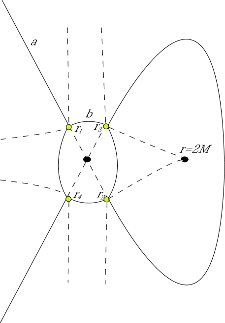
Figure 1: Zeros and poles of $Q^{2}(r)$ and for Schwarzschild black hole in the complex $r$-plane in the limit Im$(\omega)\to-\infty$. The related Stokes and anti-Stokes lines are witten by dashed lines and solid lines, respectively.

We should consider the problem concerning the “Stokes phenomenon” related to the zeros and poles of $Q^{2}$ Berry , which are written in Fig. 1 in the limit Im$(\omega)\to-\infty$. One of the important points are that the zeros of $Q^{2}$ approach the origin in the limit Im$(\omega)\to-\infty$. Near the origin, we can write as

$$Q^{2}=g^{-2}\left[\omega^{2}-\frac{4g^{2}}{r^{2}}\right]\ .$$ (18)

Since $g\to-2M/r$ for $r\to 0$ where $M$ is the mass of Schwarzschild black hole, $Q^{2}$ has four zeros. When we start the outgoing solution at the point $a$ as

$$\Psi_{a}=\Psi_{1}^{(r_{1})}\ ,$$ (19)

and proceeds along anti-Stokes lines and encircles the pole at the horizon clockwise, and turns back to $a$, we investigate what conditions are imposed to reproduce the original solution (19). For this purpose, we should account for the Stokes phenomenon associated with the zeros $r_{1}$, $r_{2}$ and $r_{3}$. For example, if we proceeds the point $a$ to $b$ passing the Stokes line, we have the solution

$$\Psi_{b}=e^{-iI}\Psi_{1}^{(r_{3})}-ie^{iI}\Psi_{2}^{(r_{3})}\ ,$$ (20)

where

$$I=\int_{r_{3}}^{r_{1}}Qdr\ .$$ (21)

For details, see Andersson . The final condition to be imposed is

$$e^{2i\Gamma}=-1-2\cos 2I\ ,$$ (22)

where

$$\Gamma=\oint Qdr\ .$$ (23)

We should also perform the same analysis for the ingoing solution near the event horizon. The result is same as (22).

Let us evaluate $\Gamma$ and $I$. $\Gamma$ is written as

$$\Gamma=-2\pi i\lim_{r\to r_{\rm H}}\frac{r-r_{\rm H}}{g}\sqrt{\omega^{2}+(g^{\prime})^{2}/4}\ ,$$ (24)

since the contributions from $V(r)$ and $-gg^{\prime\prime}/2$ disappear at the event horizon. Since the term $(g|_{r=r_{\rm H}}^{\prime})^{2}/4=4(\pi T_{\rm H})^{2}$ has finite value (Remember, (10).), we can also neglect it in the limit Im$(\omega)\to-\infty$. Then, we have

$$\Gamma = -2\pi i\lim_{r\to r_{\rm H}}\frac{r-r_{\rm H}}{g}\omega\ ,$$ (25)

$$= -2\pi i\lim_{r\to r_{\rm H}}\frac{r-r_{\rm H}}{g^{\prime}(r-r_{\rm H})}\omega=-i\frac{\omega}{2T_{\rm H}}\ .$$

Notice that this result does not depend on species of black holes which becomes important later.

To integrate $I$, we define

$$y=\frac{\omega r^{2}}{4M}\ .$$ (26)

From (18), we can perform the integral $I$ as

$$I=-\int_{-1}^{1}\sqrt{1-\frac{1}{y^{2}}}dr=\pi\ .$$ (27)

By substituting (25) and (27) into (22), we have (7) as derived in previous papers.

Next, we consider generalization of the above argument by exmplifying the case in dilatonic black hole. The crux of the point we now show is that $Q^{2}(r)$ for dilatonic black holes have two second order poles and four zeros in the limit Im$(\omega)\to-\infty$ which is qualitatively same as Schwarzschild black hole. Dilatonic black hole can be expressed using the coordinate GM-GHS

$$ds^{2}=-\lambda^{2}(\rho)dt^{2}+\frac{1}{\lambda^{2}}d\rho^{2}+r^{2}(\rho)d\Omega^{2}\ ,$$ (28)

where

$$\lambda^{2} = \left(1-\frac{\rho_{+}}{\rho}\right)\left(1-\frac{\rho_{-}}{\rho}\right)^{(1-\alpha^{2})/(1+\alpha^{2})}\ ,$$ (29)

$$r = \rho\left(1-\frac{\rho_{-}}{\rho}\right)^{\alpha^{2}/(1+\alpha^{2})}\ .$$ (30)

$\rho_{+}$, $\rho_{-}$ and $\alpha$ are the event horizon, the “inner horizon”, and the dilaton coupling, respectively. We can see from (30) that the “inner horizon” corresponds to the origin in the area radius.

By comparing (28) and (8), we obtain

$$g(r) = \left(1-\frac{\rho_{+}}{\rho}\right)\left(1-\frac{\rho_{-}}{\rho}\right)^{1/(1+\alpha^{2})}\times$$ (31)

$$\left(1+\frac{\alpha^{2}}{1+\alpha^{2}}\frac{\rho_{-}}{\rho-\rho_{-}}\right)\ ,$$

$$e^{-\delta} = \left(1-\frac{\rho_{-}}{\rho}\right)^{-\alpha^{2}/(1+\alpha^{2})}\times$$ (32)

$$\left(1+\frac{\alpha^{2}}{1+\alpha^{2}}\frac{\rho_{-}}{\rho-\rho_{-}}\right)^{-1}\ .$$

At first glance, it is not evident whether or not zeros of $Q^{2}$ approach the origin in the limit Im$(\omega)\to-\infty$. However, we can find from (31) and (32) that $e^{-\delta}$ and $g(r)$ do not show singular behavior for $r\neq 0$, $r_{\rm H}$ ($\rho\neq\rho_{-}$, $\rho_{+}$) as it is expected from the fact that dilatonic black hole is a single-horizon black hole. Thus, zeros approaches the origin as in the Schwarzschild case. We evaluate $g(r)$ in the limit $r\to 0$, which is

$$g(r)\simeq\frac{\alpha^{2}}{1+\alpha^{2}}\frac{\rho_{-}-\rho_{+}}{(\rho-\rho_{-})^{\frac{\alpha^{2}}{1+\alpha^{2}}}\rho^{\frac{1}{1+\alpha^{2}}}}\ .$$ (33)

If we substitute (30) in this relation, we obtain

$$g(r)\simeq\frac{\alpha^{2}}{1+\alpha^{2}}\frac{\rho_{-}-\rho_{+}}{r}\ .$$ (34)

Using this asymptotic relation to (16), we have $Q^{2}(r)=R-1/(4r^{2})$ again for $\Psi$ to behave near the origin appropriately. Then, we have the form (18) near the origin and using the fact that dilatonic black hole has one horizon, we find that $Q^{2}(r)$ have four zeros and two second order poles as in Schwarzschild black hole.

Therefore, the WKB condition to obtain the global solution is quite analogous to the case in Schwarzschild black hole and is written as (22). As we noted above, the expression (25) is not also changed in dilatonic black hole. The nontrivial factor is $I$. However, since only difference of $g(r)$ in (34) from Schwarzschild case is its coefficient, if we define

$$y=\frac{\omega r^{2}}{\frac{2\alpha^{2}}{1+\alpha^{2}}(\rho_{+}-\rho_{-})}\ ,$$ (35)

we can also perform the integral $I$ as (27). Thus, we obtain (7) again which is the realization of the conjecture in Visser ; Pad .

As for scalar and electromagnetic perturbations, we can perform them quite analogously. Using the asymptotic behavior

$$R(r)\simeq\frac{(1-k)(1+k)}{r^{2}}-\frac{3}{4r^{2}}\ ,$$ (36)

in the limit $r\to 0$, we obtain

$$e^{2i\Gamma}=-1-2\cos 2\pi k\ ,$$ (37)

where $k=0$, $1$ for scalar and electromagnetic perturbations, respectively. Thus, (7) also holds for scalar perturbations and the real part of electromagnetic perturbations disappears as for the case in Schwarzschild black hole.

For even parity gravitational perturbations of dilatonic black hole, isospectrality between odd and even parity mode does not hold and the corresponding basic equation becomes complicated as shown in Ref. Ferrari . However, there remains a possibility that isospectrality is restored in the highly damped mode. This is under investigation.

From the observation for the case in dilatonic black hole, the important things are: (i) the number of poles in $Q^{2}$ which is restricted to two in the single-horizon black holes. (ii) the number of zeros in $Q^{2}$ near the origin. (iii) asymptotically flatness that guarantees our boundary conditions. Therefore, if we turn back the case for higher dimensional Schwarzschild black hole in Ref. Motl ; Kuns ; Birm ; Lemos , it is not difficult to extend the formula (7) for single-horizon black holes which behave near the origin as

$$g(r)\simeq\frac{C}{r^{n}}\ ,$$ (38)

where $C$ and $n$ are the constant and the natural number, respectively. Unfortunately, since black holes with non-Abelian fields, which have one horizon in general, show complicated behavior near the origin Gal'tsov ; Maison ; Higgs ; dilaton ; Tamaki , we need further analysis to include these cases.

Conclusion and discussion. We investigated the highly damped quasinormal mode of single-horizon black holes and obtained the relation (7) for dilatonic black hole and considered the possibility of its generality. Our results are important since we supply the first example which shows (7) for black holes with matter fields. They suggest the generality of (7) in single-horizon black holes. Then, what we think about the confrontation in determining the Immirzi parameter $\gamma$ and the case in multi-horizon black holes ? It would be worth examining the present proposals Alekseev ; Corichi2 ; Corichi3 since the results $j_{\rm min}$ and $\gamma$ in both cases (would) turn out to be general for single-horizon black holes, and are too close to ignore and suggest some relations.

First, the possibility of modified area spectrum in Ref. Alekseev is not correct. Notice that the physical state does not change by adding or removing closed loops with $j=0$. The problem is that $j=0$ spin network has nonzero eigenvalue for the area operator. That is, we can obtain different eigenvalues for the area to the same physical state Corichi3 . Thus, we cannot accept this possibility.

The mechanism that prohibits the transition $j=1/2$ by the fermion conservation is important Corichi2 . This implies $j_{\rm min}=1$ if we consider the dynamical process in the area change. However, we should recongnize that $j_{\rm min}$ in (2) means the statistically dominant element which does not necessarily coincide with the former. The drawback in Ref. Corichi2 is that we can not prohibits the existence of $j=1/2$ edges puncturing the horizon as it was already pointed out. Therefore, it is important to investigate the mechanisim that suppress (or prohibit) $j=1/2$ punctures. For the supersymmetric case, this mechanism would exist as discussed in Ref. Ling .

However, there is another possibility. In our opinion, the discussion in the quasinormal modes is like the old quantum theory and its description is within the general relativity. Thus, the above confrontation and the appearent discrepancy for multi-horizon black holes may be caused by this temporal description. If we can appropriately consider the problem corresponding to the quasinormal modes in the LQG, these may be solved. It is one of the directions we are seeking for.

It is also important to consider other correspondence as done in BTZ black hole in Ref. BTZ . In this case, identification of the real part of the quasinormal frequencies with the fundamental quanta of black hole mass and angular momentum leads to the quantum behavior of the asymptotic symmetry algebra. At present, their relation to the loop quantum gravity is not clear. It is also the important direction we should seek for.

Of course, there are problems we should solve before going to the consideration above. We need to prove the case for single-horizon black holes in possibly general form. We must also include the case for the even parity mode. They are the work we are now considering.

Acknowledgement. Special thanks to Hajime Sotani, Jiro Soda, Shijun Yoshida, and Yoshiyuki Morisawa for useful discussion. This work was supported in part by Grant-in-Aid for Scientific Research Fund of the Ministry of Education, Science, Culture and Technology of Japan, 2003, No. 154568 (T.T.). This work was also supported in part by a Grant-in-Aid for the 21st Century COE “Center for Diversity and Universality in Physics”.

References

- (1) C. Rovelli and L. Smolin, Phys. Rev. D 52, 5743 (1995).
- (2) C. Rovelli and L. Smolin, Nucl. Phys. B 442, 593 (1995); Erratum, ibid., 456, 753 (1995).
- (3) A. Ashtekar and J. Lewandowski, Class. Quantum Grav. 14, A55 (1997).
- (4) G. Immirzi, Nucl. Phys. Proc. Suppl. B 57, 65 (1997).
- (5) A. Ashtekar, A. Corichi, and K. Krasnov, Adv. Theor. Math. Phys. 3, 418 (1999).
- (6) A. Ashtekar, J. Baez, A. Corichi, and K. Krasnov, Phys. Rev. Lett. 80, 904 (1998).
- (7) For review, see, e.g., M. Bojowald and H. A. Morales-Técotl, gr-qc/0306008.
- (8) O. Dreyer, Phys. Rev. Lett. 90, 081301 (2003).
- (9) J. D. Bekenstein, Lett. Nuovo Cimento 11, 467 (1974).
- (10) S. Hod, Phys. Rev. Lett. 81, 4293 (1998).
- (11) L. Motl, Adv. Theor. Math. Phys. 6, 1135 (2003); L. Motl and A. Neitzke, ibid., 7, 307 (2003).
- (12) N. Andersson and C. J. Howls, Class. Quantum Grav. 21, 1623 (2004).
- (13) A. Alekseev, A. P. Polychronakos, and M. Smedback, Phys. Lett. B 574, 296 (2003); A. P. Polychronakos, Phys. Rev. D 69, 044010 (2004).
- (14) A. Corichi, Phys. Rev. D 67, 87502 (2003).
- (15) R. K. Kaul and S. K. Rama, Phys. Rev. D 68, 24001 (2003).
- (16) A. Corichi, gr-qc/0402064.
- (17) Y. Ling and L. Smolin, Phys. Rev. D 61, 04408 (2000); Y. Ling and H. Zhang, Phys. Rev. D 68, 101501 (2003).
- (18) A. J. M. Medved, D. Martin, and M. Visser, Class. Quantum Grav. 21, 1393 (2004); ibid., 2393 (2004).
- (19) T. Padmanabhan, Class. Quantum Grav. 21, L1 (2004); T. R. Choudhury and T. Padmanabhan, Phys. Rev. D 69, 064033 (2004).
- (20) R. A. Konoplya, Phys. Rev. D 66, 044009 (2002); V. Cardoso, R. A. Konoplya, and J. P. S. Lemos, Phys. Rev. D 68, 044024 (2003); V. Cardoso and J. P. S. Lemos, Phys. Rev. D 67, 084020 (2003); A. Maassen van den Brink, Phys. Rev. D 68, 047501 (2003); R. A. Konoplya and A. Zhidenko, hep-th/0402080; V. Cardoso, J. Natário, and R. Schiappa, hep-th/0403132.
- (21) S. Yoshida and T. Futamase, Phys. Rev. D 69, 064025 (2004).
- (22) E. Berti and K. D. Kokkotas, Phys. Rev. D 68, 044027 (2003).
- (23) E. Berti, V. Cardoso, K. D. Kokkotas, and H. Onozawa, Phys. Rev. D 68, 124018 (2003); E. Berti, V. Cardoso, and S. Yoshida, gr-qc/0401052.
- (24) G. W. Gibbons and K. Maeda, Nucl. Phys. B 298, 741 (1988); D. Garfinkle, G. T. Horowitz and A. Strominger, Phys. Rev. D 43, 3140 (1991).
- (25) V. Ferrari, M. Pauri, and F. Piazza, Phys. Rev. D 63, 064009 (2001); R. Moderski and M. Rogatko, Phys. Rev. D 63, 064009 (2001); R. A. Konoplya, Gen. Relativ. Gravit. 34, 329 (2002); R. A. Konoplya, Phys. Rev. D 66, 084007 (2002).
- (26) M. Karlovini, Class. Quantum Grav. 19, 2125 (2002).
- (27) M. V. Berry, Proc. Roy. Soc. A 422, 7 (1989).
- (28) G. Kunstatter, Phys. Rev. Lett. 90, 161301 (2003).
- (29) D. Birmingham, Phys. Lett. B 569, 199 (2003).
- (30) V. Cardoso, J. P. S. Lemos, and S. Yoshida, Phys. Rev. D 69, 044004 (2004).
- (31) E. E. Donets, D. V. Gal’tsov, and M. Yu. Zotov, Phys. Rev. D 56, 3459 (1997); D. V. Gal’tsov, E. E. Donets, and M. Yu. Zotov, gr-qc/9712003; ibid., gr-qc/9712024; ibid., hep-th/9709181; ibid., JETP Lett. 65, 895 (1997).
- (32) P. Breitenlohner, G. Lavrelashvili, and D. Maison, Nucl. Phys. B 524, 427 (1998); ibid., gr-qc/9708036; ibid., gr-qc/9711024.
- (33) D. V. Gal’tsov, E. E. Donets, gr-qc/9706067.
- (34) O. Sarbach, N. Straumann, and M. S. Volkov, gr-qc/9709081.
- (35) T. Tamaki, K. Maeda, and T. Torii, Phys. Rev. D 64, 084019 (2001).
- (36) D. Birmingham, S. Carlip, and Y. Chen, Class. Quantum Grav. 20, L239 (2003); D. Birmingham and S. Carlip, Phys. Rev. Lett. 92, 111302 (2004).