hep-th/0405118

NSF-KITP-04-53

Seiberg Duality is an Exceptional Mutation

Christopher P. Herzog
KITP, UCSB,

Santa Barbara, CA 93106, U.S.A.

herzog@kitp.ucsb.edu

Abstract

The low energy gauge theory living on D-branes probing a del Pezzo singularity of a non-compact Calabi-Yau manifold is not unique. In fact there is a large equivalence class of such gauge theories related by Seiberg duality. As a step toward characterizing this class, we show that Seiberg duality can be defined consistently as an admissible mutation of a strongly exceptional collection of coherent sheaves.

May 2004

1 Introduction

We study the action of Seiberg duality on strongly coupled gauge theories with gravity duals. Our examples are constructed from D-branes probing del Pezzo singularities of a non-compact Calabi-Yau manifold.

These del Pezzo constructions are interesting examples of gauge/gravity duality because they exhibit several new features not observed in simpler models. For example, [1, 2, 3] gave evidence that the gauge theories for these del Pezzo models often have duality walls. In other words, the gauge theories cannot not be defined at energies higher than the scale of the wall. In [3], the authors argue that the renormalization group flows for these models not only have walls but also can be chaotic.

The motivation for this paper comes partially from a desire to better understand the duality walls and chaotic renormalization group flows of these del Pezzo theories. In order to follow the renormalization group flow, the authors of [2, 3] relied on ideas of Klebanov and Strassler (KS) [4]. KS studied D-branes probing a conifold singularity and discovered that the renormalization group flows could be continued past strong coupling by looking at the Seiberg dual. One crucial difference between the KS paper and the del Pezzo examples is that while the Seiberg dual of the conifold gauge theory is essentially the same gauge theory, Seiberg duality acting on a del Pezzo gauge theory produces, typically, an infinite tree of new theories. To understand duality walls and chaotic renormalization group flows, we first need a better understanding of the different possible Seiberg dual theories.

A second motivation for the present paper is a desire to clear up some puzzles in the immense literature on Seiberg duality for del Pezzos. In addition to Seiberg’s original gauge theory analysis [5] (see [6] for a review), here are four conjectured alternate ways of understanding the equivalence:

1. Toric Duality: Using toric geometry to derive del Pezzo gauge theories, the authors of [7, 8] noticed that a phenomenon called toric duality could example by example be understood as Seiberg duality. However, not all del Pezzos are toric.

2. Picard-Lefschetz Monodromy: The authors of [8, 9, 10] pointed out that certain but not all Picard-Lefschetz monodromies in the mirror geometry were Seiberg dualities.

3. Mutation: Using exceptional collections of sheaves to generate the gauge theory, [9] and [11] noticed that certain combinations of mutations (or braiding operations on the collections) were Seiberg dualities. The combinations that were not mutations were labelled partial Seiberg dualities. On an example by example basis, partial Seiberg dualities tend to produce pathological gauge theories [12, 13].

4. Tilting Equivalences: The low energy gauge theory on these D-brane configurations can be described by a quiver with relations. There is a derived category which can be constructed from the quiver. Berenstein and Douglas [14] conjecture that Seiberg duality can be understood as a tilting equivalence of the quiver derived category. This idea was later developed by [15, 16].

This brief list makes several problems clear. In all this early work, although some Seiberg dualities had alternate interpretations, it was never clear that all Seiberg dualities could be understood using some other framework. It was also not clear what role if any partial Seiberg dualities should play. Here are two important questions: How general is the equivalence between Seiberg duality and any item on this list? How precisely are the various items on this list related to each other?

In this paper, we show that mutation is a consistent alternate way of thinking about Seiberg duality for all our del Pezzo examples. Our results suggest a close relationship between mutation and tilting equivalences.

As a step toward classifying all possible Seiberg dual theories for del Pezzos, we find evidence that all these theories are well split. A precise definition begins section 5; here we give a simple but intriguing consequence for the superpotential. Well split means that there is a cyclic ordering of the $SU(N)$ gauge groups which any possible superpotential term respects.

1.1 Statement of Results

Our strongly coupled gauge theories are engineered from a ten dimensional geometry $\mathbb{R}^{3,1}\times\mathbf{X}$ where $\mathbb{R}^{3,1}$ is four dimensional Minkowski space and $\mathbf{X}$ is a three complex dimensional Calabi-Yau. We consider a severely restricted class of $\mathbf{X}$. Let $\mathcal{B}$ be a del Pezzo surface, i.e. $\mathbb{P}^{2}$, $\mathbb{P}^{1}\times\mathbb{P}^{1}$, or $\mathbb{P}^{2}$ blown up at $n$ points where $1\leq n\leq 8$. Our $\mathbf{X}$ is a complex line bundle over $\mathcal{B}$. (In particular, we take the canonical line bundle $\mathcal{O}(K)$ over $\mathcal{B}$.)

The D-branes in this geometry fill $\mathbb{R}^{3,1}$ and wrap holomorphic cycles in $\mathbf{X}$. (We work with type IIB string theory.) We assume there is a locus in the Kaehler moduli space of $\mathbf{X}$ where $\mathcal{B}$ shrinks to zero size. At this point in the moduli space, we expect an enhanced gauge symmetry for D-branes wrapping cycles in $\mathcal{B}$, essentially because of all the strings between the D-branes that become massless. In the case of $\mathbb{P}^{2}$, this locus of enhanced symmetry corresponds to the point in moduli space where $\mathbf{X}$ becomes the orbifold $\mathbb{C}^{3}/\mathbb{Z}_{3}$ [17]. By an abuse of notation, we shall continue to call this locus the “orbifold point” for general del Pezzos. However, it is important to note that in general the locus may contain more than one point and $\mathbf{X}$ may not be an orbifold on this locus.

Kontsevich [18] conjectured and later Douglas and collaborators [17, 19, 20] gave further support to the idea that these holomorphically wrapped D-branes are objects in the derived category of coherent sheaves $D^{\flat}(\mathbf{X})$. Bondal has shown that exceptional collections of coherent sheaves on the del Pezzos generate $D^{\flat}(\mathcal{B})$ [21]. In this esoteric mathematical context, it is not too surprising that exceptional collections should play a vital role in understanding the low energy gauge theories on these D-branes. Indeed, Cachazo, Fiol, Intriligator, Katz, Vafa [9], and later Wijnholt [11] proposed a recipe for writing down a gauge theory given an exceptional collection. It is this recipe that we analyze in detail using the lens of Seiberg duality.

In an earlier paper [13], we found that Seiberg duality could be defined in terms of mutations if the D-brane configuration (or exceptional collection) was well split. In order to have a consistent definition, we conjectured in [13] that the Seiberg dual of a well split quiver was well split.

Taken together, the two principal results of this paper, Theorems 5.3 and 5.4, allow a consistent definition of Seiberg duality in terms of mutations of strongly exceptional collections and prove a weaker version of the well split conjecture. Theorem 5.3 identifies a subset of well split exceptional collections, namely exceptional collections which are not only strongly exceptional but which also generate something called a strong helix. Theorem 5.4 states that the Seiberg dual of an exceptional collection which generates a strong helix is another exceptional collection which also generates a strong helix.

These two results allow us consistently to ignore the problematic partial Seiberg dualities mentioned above. The types of gauge theories (not well split) and exceptional collections (not strongly exceptional) that arise from partial Seiberg dualities, never arise from performing Seiberg duality.

Strong helices have appeared in the mathematics literature before. Bondal [21] calls them admissible helices. The condition that a D-brane configuration generates a strong helix is a statement about the kinds of open strings between the D-branes (or equivalently Ext maps between the sheaves in the exceptional collection).

There is a separate more mathematical way of understanding our results. Bondal [21] defines admissible mutations to be those which preserve the strongly exceptional property of the D-brane configuration. Thus, we have demonstrated that Seiberg dualities can be understood as admissible mutations.

To make the connection between well split and the strong helix property, we introduce an intermediate notion, dubbed $\mbox{Ext}^{1,2}$ which, though technical, is a more obvious physical constraint on the D-branes than strongly exceptional. We will not give a precise definition of $\mbox{Ext}^{1,2}$ until section 5, but we will be able partially to elucidate the physics of it in section 2. Two key auxiliary results in this paper are 1) Lemma 5.5 which states that $\mbox{Ext}^{1,2}$ implies the collection is well split and 2) Propositions 5.10 and 5.11 which imply $\mbox{Ext}^{1,2}$ is equivalent to the strong helix property.

1.2 Reading Map

This paper is meant to be read by both mathematicians and physicists. As a result, there are some sections which may be less interesting for one or the other half of the intended audience. Section 2 is intended primarily for a physics audience interested in understanding why the derived category is useful for studying gauge theory and is drawn largely from other sources (see for example [24]). Section 3 sets up the exceptional collection machinery with a level of rigor hopefully acceptable to mathematicians and is also drawn from other sources (see for example [25]). Section 4, which should be interesting to both physicists and mathematicians, describes how to convert an exceptional collection on a del Pezzo into a quiver gauge theory, a recipe worked out in [9, 11, 26]. Section 5 contains the proofs of the new results described in the introduction concerning the $\mbox{Ext}^{1,2}$ and strongly exceptional conditions. The penultimate section contains a discussion of how our exceptional collection definition of Seiberg duality matches the original gauge theory definition.

2 Gauge Theories from B-Branes

In this section, we make more precise the way in which gauge theories arise from D-brane configurations. The material below is drawn largely from other sources [17, 19, 20, 27, 28] (for a recent review, see for example [24]), but we include it for coherence and completeness.

Our universe consists of D3-, D5-, and D7-branes in $\mathbb{R}^{3,1}\times\mathbf{X}$ where $\mathbf{X}$ is a noncompact Calabi-Yau three-fold. We want to think of our gauge theory as living in $\mathbb{R}^{3,1}$, and so our D-branes span these directions. To preserve ${\mathcal{N}}=1$ supersymmetry, we take the remaining transverse directions of the D-branes to lie on holomorphic cycles in $\mathbf{X}$. If we think only in terms of $\mathbf{X}$, we have B-branes.

The gauge theory is the low energy world-volume description of the D-branes. In particular, we only keep the massless degrees of freedom, the degrees of freedom that morally at least correspond to zero-length strings joining the D-branes. But we need to be more precise.

First, we need a more precise definition of these D3-, D5-, and D7-branes. Inside $\mathbf{X}$, they are submanifolds with some additional data. If we think of the D-brane intrinsically, independent of its embedding, the additional data is a vector bundle. However, once we put the D-brane back in its ambient space $\mathbf{X}$, we are forced into using the language of coherent sheaves.

For example, consider the trivial line bundle ${\mathcal{O}}$. Global sections of $\mathcal{O}$ are holomorphic functions on $\mathbf{X}$. Consider also ${\mathcal{O}}(-D)$. The global sections of $\mathcal{O}(-D)$ have the analog of a single pole on the submanifold (or divisor) $D$. There is clearly a map

$${\mathcal{O}(-D)}\rightarrow{\mathcal{O}}\ ,$$ (1)

which is given by multiplying sections of $\mathcal{O}(-D)$ by sections which vanish on $D$. Morally, the cokernel of such a map, which we denote ${\mathcal{O}}_{D}$, is a D-brane, i.e. the set of holomorphic functions on a submanifold (or divisor) $D$. However, such an object is not a vector bundle in $\mathbf{X}$. Mathematicians would say that the kernel (or cokernel) of a map between vector bundles does not necessarily exist while the kernel of maps between coherent sheaves does.

As a first pass, then, D-branes correspond to coherent sheaves on $\mathbf{X}$. It turns out, however, that neither sheaves nor vector bundles are quite good enough. Physically, we also need to be able to describe anti-branes. An anti-brane should correspond to an “inverse” sheaf with the opposite charges, but taking the inverse of a sheaf is difficult. Instead, mathematicians introduce the notion of the derived category of coherent sheaves, $D^{\flat}(\mathbf{X})$ where inverting is more natural. In the derived category, sheaves get promoted to complexes that are zero everywhere except at one position. Let $\delta$ be the map that takes a sheaf $E$ into an object in $D^{\flat}(\mathbf{X})$:

$$\delta E\equiv\cdots\to 0\to E\to 0\to\cdots\ .$$ (2)

Although the position of $E$ in a sequence has no meaning, once we introduce other sheaves (or D-branes), we need to keep track of which elements in the sequence are nonzero. Thus, $\delta E[n]$ is the complex with $E$ shifted $n$ places to the left. In this language, $\delta E$ shifted an odd number of places is an antibrane of $\delta E$. To sum up, we have found that B-type D-branes are objects, i.e. complexes, in $D^{\flat}(\mathbf{X})$.

Next, we need a better definition of the massless degrees of freedom corresponding to zero-length strings. Massless degrees of freedom often come from zero modes of a system, which are topological in nature, suggesting we look at the cohomology of the D-branes. Take two D7-branes corresponding to the line bundles $\mathcal{O}(E)$ and $\mathcal{O}(F)$. Someone truly inspired might guess (correctly) that the massless degrees of freedom should come from

$$H^{(0,k)}(\mathcal{O}(F)\otimes\mathcal{O}(E)^{*})$$ (3)

for some $k$. However, such a guess, while good for vector bundles, is insufficient for sheaves. Luckily mathematicians have introduced a more general notion of cohomology for sheaves called Ext. For vector bundles, we find

$$H^{(0,k)}(\mathcal{O}(F)\otimes\mathcal{O}(E)^{*})=\mbox{Ext}^{k}(\mathcal{O}(E),\mathcal{O}(F))\ .$$ (4)

On the three-fold $\mathbf{X}$, our candidate massless degrees of freedom correspond to $\mbox{Ext}^{k}$ where $k=0$, 1, 2, or 3. There is a notion of Serre duality for Ext groups. On $\mathbf{X}$, Serre duality tells us that

$$\mbox{Ext}^{k}(E,F)=\mbox{Ext}^{3-k}(F,E)^{*}\ .$$ (5)

As a last step in identifying candidate massless degrees of freedom, we need to lift Ext to $D^{\flat}(\mathbf{X})$, which fortunately has also been worked out by mathematicians. One finds that

$$\mbox{Ext}^{k}(E,F)=\mbox{Hom}^{k-p+q}_{D^{\flat}(\mathbf{X})}(\delta E[p],\delta F[q])\$$ (6)

where no summation on $p$ and $q$ is implied.

Armed with a categorical description of D-branes and some candidates for massless degrees of freedom, we need to check whether or not these degrees of freedom are actually massless. The masses of the strings depend on the Kaehler moduli space of $\mathbf{X}$. Strings that are massive at one point in Kaehler moduli space may become massless or even tachyonic as we move to another point! In fact, more than the masses of the strings is at stake here. A tachyonic string indicates the original pair of D-branes is unstable and will condense to form a bound state.

The masses are most easily checked at the large volume point in the Kaehler moduli space of $\mathbf{X}$. However, we will eventually need to compute the masses at the analog of the orbifold point. Recall the case where $\mathbf{X}$ is the complex line bundle $\mathcal{O}(-3)$ over $\mathbb{P}^{2}$. The total space is Calabi-Yau. At the large volume point, the $\mathbb{P}^{2}$ gets very large. The orbifold point is $\mathbb{C}^{3}/\mathbb{Z}_{3}$. For a general del Pezzo, at the analog of the orbifold point, $\mathcal{B}$ should shrink to zero size and we expect there to be extra massless open strings which enhance the gauge symmetry of D-branes wrapping cycles of $\mathcal{B}$.

In general, we can define the D-brane charge of a sheaf $E$

$$Z(E)=\int_{\mathbf{X}}e^{-B-iJ}\mbox{ch}(E)\sqrt{\mbox{Td}(\mathbf{X})}+\ldots$$ (7)

where $\mbox{Td}(\mathbf{X})$ is the Todd class of $\mathbf{X}$, $B+iJ$ is the complexified Kaehler form, and the $\ldots$ are instanton corrections which become more and more important as we move away from large volume (large $J$). Fortunately, the Picard-Fuchs equations and the mirror geometry usually allow one to calculate $Z(E)$ numerically. We define the overall grading of the brane

$$\xi(E)=\frac{1}{\pi}\arg Z(E)\mod 2\ .$$ (8)

One can also define $Z$ and $\xi$ in the derived category. At large volume, the categorical grading $n$ of $\delta E[n]$ multiplies $Z(E)$ by $(-1)^{n}$:

$$Z(\delta E[n])=e^{i\pi n}Z(E)\ .$$ (9)

The mass of the mode in $\mbox{Hom}_{D^{\flat}(\mathbf{X})}^{k}(A,B)$ is given by

$$M^{2}=\frac{1}{2}(\xi(B)-\xi(A)+k-1)\ .$$ (10)

The formula (10) is confusing in that $M^{2}$ changes as we move away from the large volume point. At large volume, we might have a D7-brane anti-brane pair and a corresponding tachyon with $M^{2}=-1/2$. However, as we move to the “orbifold point”, instanton corrections can align the two $\xi$, leaving a massless field.

Now, we analyze the masses at the analog of the orbifold point. At such a supersymmetric locus of points, all the gradings $\xi(A_{i})$ of the branes should be aligned, i.e. $\xi(A_{i})=\xi(A_{j})$ $\forall i,j$ [17, 24]. We will assume in all that follows that such a supersymmetric locus of points exists. This assumption lets us ignore the Picard-Fuchs equations and other subtleties of computing $Z(E)$.

As a result of this assumption, for $\mbox{Hom}_{D^{\flat}}^{k}(A,B)$, $k=2$ or 3, the mass is positive and the corresponding degree of freedom should be absent in the low energy theory on the collection of D-branes at the “orbifold point”. For $k=1$, we find a massless scalar mode. For $k=0$, we find a tachyon! The ${\mathcal{N}}=1$ supersymmetry tells us that our fields should fall into chiral or vector multiplets.

We recall a little elementary superstring theory and move beyond topological reasoning. In quantizing the string in flat space, we used the GSO projection to get rid of the tachyon. In the present context, we can use the GSO projection to eliminate the ground state string modes corresponding to $\mbox{Hom}_{D^{\flat}}^{0}(E,F)$ and $\mbox{Hom}_{D^{\flat}}^{2}(E,F)$. In this way, we eliminate all the tachyons.

Let’s consider what kinds of fields are left. Take $\mbox{Hom}_{D^{\flat}}^{0}(E,E)$. Although the ground state tachyon is projected out, just as in the more familiar context of quantizing superstrings in $\mathbb{R}^{9,1}$, there is an excited massless string state corresponding to a gauge boson (and, filling out the $\mathcal{N}=1$ multiplet, a gaugino). For $\mbox{Hom}_{D^{\flat}}^{1}(E,E)$, we get adjoint matter fields. For $\mbox{Hom}_{D^{\flat}}^{1}(E,F)$, we get matter fields transforming in the fundamental of one gauge group and the antifundamental of another.

On the other hand, $\mbox{Hom}_{D^{\flat}}^{0}(E,F)$, $E\neq F$, is problematic. Although the ground state is projected out, the first excited state is a gauge field transforming in the bifundamental representation of the gauge groups associated with $E$ and $F$. Gauge fields by definition should transform in the adjoint representation of a Lie group. Moreover, this Lie group should be a direct product of simple Lie groups and $U(1)$ factors. The gauge groups associated with $E$ and $F$ will be of type $SU(N)$. The bifundamental representation of $SU(N)\times SU(M)$ is the adjoint representation of some Lie group, but that Lie group does not have this direct product structure. (See however [29] for a different perspective on these fields.) It is precisely these types of fields that can arise under the partial Seiberg dualities discussed in the introduction.

We are now in a position to elucidate in part the $\mbox{Ext}^{1,2}$ condition. One consequence of the $\mbox{Ext}^{1,2}$ condition is that for $E\neq F$, $k$ in $\mbox{Hom}^{k}_{D^{\flat}}(E,F)$ is either one or two. Thus, these weird bifundamental gauge fields will never appear and will never be produced by Seiberg duality. In other words, we can consistently ignore all the D-brane configurations which give rise to bifundamental gauge fields.

3 Exceptional Sheaves on del Pezzos

We are interested in exceptional collections of coherent sheaves $E$ supported on a del Pezzo surface $\mathcal{B}$. The standard mathematical reference, from which we draw much of this section, is [25].

Definition 3.1.

A sheaf $E$ is called exceptional if $\mbox{Hom}(E,E)\cong\mathbb{C}$ and $\mbox{Ext}^{i}(E,E)=0$ for $i>0$.

Recall that $\mbox{Hom}\equiv\mbox{Ext}^{0}$. In gauge theory language, we would associate a gauge group to each sheaf. Exceptional sheaves have no adjoint matter. In [30] it is proven that an exceptional sheaf $E$ on a del Pezzo is either a vector bundle or a torsion sheaf of the form $\mathcal{O}_{\ell}(m)$ where $\ell$ is an exceptional curve.

Definition 3.2.

An exceptional collection is an ordered set of exceptional sheaves $(E_{1},E_{2},\ldots,E_{n})$ with the following additional properties:

1. $\mbox{Ext}^{k}(E_{i},E_{j})=0$ $\forall k$ if $i>j$;

2. $\mbox{Ext}^{k}(E_{i},E_{j})=0$ for all but at most one $k$ if $i<j$.

For gauge theories, the Ext maps between sheaves correspond to bifundamental matter fields. The exceptional collection condition implies that the matter associated with any particular sheaf/gauge group is chiral.

Definition 3.3.

A strongly exceptional collection is an exceptional collection such that only $\mbox{Hom}(E_{i},E_{j})$ is nonzero.

Kuleshov and Orlov (see section 2.11 of [30]) demonstrated that for del Pezzo surfaces, for an exceptional pair $(E,F)$, the maps $\mbox{Ext}^{i}(E,F)$ can be non-zero for either only Hom or only $\mbox{Ext}^{1}$.

3.1 Euler Character

We will gradually see the significance of strong exceptionality, but we remark in the meantime that the Euler character $\chi(E,F)$ makes exceptional collections relatively easy to work with:

$$\chi(E,F)\equiv\sum_{k}(-1)^{k}\dim\mbox{Ext}^{k}(E,F)\ .$$ (11)

In particular, the Euler character is an efficient tool for calculating $\dim\mbox{Ext}^{i}(E,F)$ for an exceptional pair $(E,F)$ (and hence the number of bifundamentals in the gauge theory). Riemann-Roch implies that

$$\chi(E,F) = \int_{\mathcal{B}}\mbox{ch}(E^{*})\mbox{ch}(F)\mbox{Td}(\mathcal{B})$$

$$= r(E)r(F)+\frac{1}{2}(r(E)\mbox{deg}(F)-r(F)\mbox{deg}(E))$$

$$+r(E)\mbox{ch}_{2}(F)+r(F)\mbox{ch}_{2}(E)-c_{1}(E)\cdot c_{1}(F)\$$

where we have used the Chern character of the sheaf

$$\mbox{ch}(E)=(r(E),c_{1}(E),\mbox{ch}_{2}(E))\ .$$ (12)

Also, $\mbox{Td}(\mathcal{B})=1-\frac{K}{2}+H^{2}$, where $K$ is the canonical class and $H$ is the hyperplane, with $\int_{\mathcal{B}}H^{2}=1$. Finally, the degree $\mbox{deg}(E)=(-K)\cdot c_{1}(E)$.

Definition 3.4.

We define the slope of a torsion free sheaf $E$ to be $\mu(E)=\mbox{deg}(E)/r(E)$.

The slope of a torsion sheaf $\mu(\mathcal{O}_{\ell}(m))$ is taken to be infinite.

We denote $\chi_{-}(E,F)$ to be the antisymmetric part of $\chi$

$$\chi_{-}(E,F)=r(E)\mbox{deg}(F)-r(F)\mbox{deg}(E)\ .$$ (13)

Note that for an exceptional pair $(E,F)$, $\chi_{-}(E,F)=\chi(E,F)$. For torsion free sheaves, we may write

$$\chi_{-}(E,F)=r(E)r(F)(\mu(F)-\mu(E))\ .$$ (14)

3.2 Derived Category

We denote by $D^{\flat}(\mathcal{B})$ the bounded derived category of coherent sheaves on $\mathcal{B}$. The main reason for moving to the derived category is that we will need a notion of an inverse exceptional collection, and while sheaves do not necessarily have well defined inverses, their images in the derived category do.

We can map coherent sheaves $E$ to objects in the derived category in a simple way. In particular, we denote by $\delta E$ the complex in $D^{\flat}(\mathcal{B})$ which has only one nonzero entry, $E$. We are free to shift the location of $E$ in the complex by $k$ units to the left, which we denote $\delta E[k]$. Note that

$$\mbox{Hom}_{D^{\flat}}^{k}(\delta E[i],\delta F[j])=\mbox{Hom}^{k-i+j}_{D^{\flat}}(\delta E,\delta F)=\mbox{Ext}^{k-i+j}(E,F)\ .$$ (15)

The notion of exceptionality extends naturally to $D^{\flat}(\mathcal{B})$. An object $A\in D^{\flat}(\mathcal{B})$ is called exceptional if $\mbox{Hom}^{0}_{D^{\flat}(\mathcal{B})}(A,A)\cong\mathbb{C}$ and $\mbox{Hom}^{i}_{D^{\flat}(\mathcal{B})}(A,A)=0$ for $i\neq 0$. The notion of exceptional collection generalizes as well. For a set of objects $(A_{1},A_{2},\ldots A_{n})$, $\mbox{Hom}^{k}_{D^{\flat}(\mathcal{B})}(A_{i},A_{j})=0$ for $i>j$ and $\mbox{Hom}^{k}_{D^{\flat}(\mathcal{B})}(A_{j},A_{i})=0$ for all but at most one $k$.

We define the Euler character for complexes with one nonzero element in the following way:

$$\chi(\delta E[j],\delta F[k])=(-1)^{k-j}\chi(E,F)\ .$$ (16)

3.3 Mutations

A useful way of generating new exceptional collections from old ones is mutation. We will eventually see that certain sequences of mutations are Seiberg dualities. Let $(A,B)$ be an exceptional pair of objects in $D^{\flat}(\mathcal{B})$. There exists a canonical morphism $\mbox{RHom}(A,B)\otimes A\stackrel{{\scriptstyle can}}{{\to}}B$. Let the left mutation of $B$ over $A$, denoted $L_{A}^{D}B$, be the object which completes this morphism to a distinguished triangle

$$L_{A}^{D}B[-1]\to\mbox{RHom}(A,B)\otimes A\stackrel{{\scriptstyle can}}{{\to}}B\to L_{A}^{D}B\ .$$ (17)

Equivalently, one may define right mutation as the object which completes the canonical morphism $A\to\mbox{RHom}^{*}(A,B)\otimes B$ to the distinguished triangle

$$R_{B}^{D}A\to A\to\mbox{RHom}^{*}(A,B)\otimes B\to R_{B}^{D}A[1]\ .$$ (18)

Theorem 3.5 (see for example Section 2.3 of [31]).

If $(A,B)$ is an exceptional pair in $D^{\flat}(\mathcal{B})$, then $(L_{A}^{D}B,A)$ and $(B,R_{B}^{D}A)$ are exceptional pairs in $D^{\flat}(\mathcal{B})$.

For a pair $(A,B)=(\delta E,\delta F)$, the distinguished triangle (17) will reduce to a short exact sequence of sheaves. If $\mbox{Ext}^{1}(E,F)\neq 0$, the mutation is called an extension and takes the form

$$0\to F\to L_{E}F\to\mbox{Ext}^{1}(E,F)\otimes E\to 0\ .$$ (19)

If $\mbox{Hom}(E,F)\neq 0$, we need to make sure that $L_{E}F$ is defined in such a way that $r(L_{E}F)=\pm(r(F)-\chi(E,F)r(E))\geq 0$. There are two possibilities:

$$0\to L_{E}F\to\mbox{Hom}(E,F)\otimes E\to F\to 0 \mbox{(division)}\ ,$$

$$0\to\mbox{Hom}(E,F)\otimes E\to F\to L_{E}F\to 0 \mbox{(recoil)}\ .$$

Similarly for right mutation, we find the three short exact sequences

$$0\to E\to\mbox{Hom}(E,F)^{*}\otimes F\to R_{F}E\to 0 \mbox{(division)}\ ,$$

$$0\to R_{F}E\to E\to\mbox{Hom}(E,F)^{*}\otimes F\to 0 \mbox{(recoil)}\ ,$$

$$0\to\mbox{Ext}^{1}(E,F)^{*}\otimes F\to R_{F}E\to E\to 0 \mbox{(extension)}\ .$$

In the case where $L_{F}E$ or $R_{F}E$ is torsion, there is an ambiguity in the positive rank prescription which we now eliminate. Note from our elementary discussion of torsion sheaves around (1) that we expect these torsion sheaves to show up as cokernels in short exact sequences. Thus, if $L_{F}E$ is torsion, we conclude the sequence must be a recoil while if $R_{F}E$ is torsion, then the sequence is a division.

Now we come to a crucial observation about the relation between mutation in $D^{\flat}(\mathcal{B})$ and mutation of coherent sheaves.

Proposition 3.6 (Proposition 1.8 of [32]).

If a sheaf mutation of a pair $(E,F)$ is either a recoil or an extension, then $L_{\delta E}^{D}\delta F=\delta L_{E}F$ and $R_{\delta F}^{D}\delta E=\delta R_{F}E$. For the case of division, $L_{\delta E}^{D}\delta F=\delta L_{E}F[1]$ and $R_{\delta F}^{D}\delta E=\delta R_{F}E[-1]$.

3.4 Braid Group

One can think of mutations as an action of the braid group on an exceptional collection.

We define the following maps $L_{i}$ and $R_{i}$ on an exceptional collection $\mathcal{E}=(E_{1},\ldots,E_{n})$:

$$L_{i}:(\ldots,E_{i-1},E_{i},E_{i+1},\ldots) \to (\ldots,E_{i-1},L_{E_{i}}E_{i+1},E_{i},\ldots)\ ,$$

$$R_{i}:(\ldots,E_{i-1},E_{i},E_{i+1},\ldots) \to (\ldots,E_{i-1},E_{i+1},R_{E_{i+1}}E_{i},\ldots)\ .$$

Proposition 3.7 (Section 2.3 of [31], Assertion 2.3 of [21]).

The mutations $R_{i}$ and $L_{i}$ are inverse, $R_{i}\circ L_{i}=\mbox{id}$. Moreover, right and left mutations define an action of the $n$-string braid group on $\mathcal{E}$:

$$R_{i}\circ R_{i+1}\circ R_{i}=R_{i+1}\circ R_{i}\circ R_{i+1}\;,\;\;\;L_{i}\circ L_{i+1}\circ L_{i}=L_{i+1}\circ L_{i}\circ L_{i+1}\ .$$ (20)

3.5 Helices

A helix $\mathcal{H}=(E_{i})_{i\in\mathbb{Z}}$ is a bi-infinite extension of an exceptional collection $\mathcal{E}$ defined recursively by

$$E_{i+n} = R_{E_{i+n-1}}\cdots R_{E_{i+1}}E_{i}\ ,$$

$$E_{-i} = L_{E_{-i+1}}\cdots L_{E_{n-1-i}}E_{n-i}\;\;\;i\geq 0\ .$$

such that the helix has period $n$, by which we mean

$$E_{i}=E_{n+i}\otimes K\;\;\;\;\forall i\in\mathbb{Z}\ .$$ (21)

A foundation of a helix is any subcollection of the form $(E_{m+1},\ldots,E_{m+n})$, where $m\in\mathbb{Z}$. An exceptional collection is called complete if it generates $D^{\flat}(\mathcal{B})$.

Theorem 3.8 (Theorem 4.1 of [21]).

An exceptional collection is complete if and only if it is the foundation of a helix.

A corollary that can be extracted from Bondal’s proof of the preceding theorem (and Serre duality) is that

$$L^{D}_{\delta E_{1}}L^{D}_{\delta E_{2}}\cdots L^{D}_{\delta E_{n-1}}\delta E_{n}=\delta(E_{n}\otimes K)[2]\ .$$ (22)

Helices provide us with a stronger notion of strongly exceptional which will be important for our proofs.

Definition 3.9.

A strong helix is a helix $\mathcal{H}$ such that every foundation $\mathcal{E}$ of $\mathcal{H}$ is strongly exceptional.

Remark 3.10.

Given an exceptional collection $\mathcal{E}=(E_{1},\ldots,E_{n})$, $\mathcal{E}$ generates a strong helix if and only if the slopes satisfy

$$\mu(E_{1})\leq\mu(E_{2})\leq\cdots\leq\mu(E_{n})\leq\mu(E_{1})+K^{2}\ .$$ (23)

The remark follows from (21). In the forward direction, we find that $\mathcal{E}$ must be strongly exceptional. Therefore, the first $n-1$ inequalities follow. We could also choose a different foundation which included $E_{n}\otimes K$ and $E_{1}$ as neighbors in the collection. Then the last inequality follows because tensoring with $K$ subtracts $K^{2}$ from the slope of the sheaf. In the reverse direction, we know that all foundations of the helix can be generated by tensoring the sheaves in $\mathcal{E}$ with $K$ the appropriate number of times. Given any foundation, $n-1$ of the $n$ inequalities above are sufficient to guarantee that the foundation is strongly exceptional. (Note we have departed from the conventions of Bondal [21] here, who calls such helices admissible.)

4 Quiver Gauge Theories

Definition 4.1.

A quiver is a collection of nodes (or vector spaces) and arrows (or maps between the vector spaces).

For nodes $i$ and $j$, we denote a map from vector space $V_{i}$ to $V_{j}$ as $X_{ij}$. A quiver with relations is a quiver where certain compositions of maps are identified.

Definition 4.2.

A ${\mathcal{N}}=1$ supersymmetric quiver is a quiver with relations such that all the relations are generated by a superpotential $W$ and are of the form

$$\frac{\partial W}{\partial X_{ij}}=0\ .$$ (24)

Moreover, the superpotential must be a polynomial in the $X_{ij}$ and correspond to a sum over loops in the quiver.

To each exceptional collection of sheaves $\mathcal{E}=(E_{1},\ldots,E_{n})$, we can associate a supersymmetric quiver in the following way. To calculate the number of bifundamentals or maps between the nodes, we first produce the left-dual collection or gauge theory collection

$$\mathcal{E}^{Q}=(E_{n}^{\vee},\ldots,E_{1}^{\vee})=(L^{D}_{\delta E_{1}}\cdots L^{D}_{\delta E_{n-1}}\delta E_{n},\ldots,L^{D}_{\delta E_{1}}\delta E_{2},\delta E_{1})\ .$$ (25)

Note that this collection is dual in the sense of the Euler character:

$$\chi(E_{i},E_{j}^{\vee})=\delta_{ij}\ .$$ (26)

We define the upper triangular matrix

$$S_{ij}=\chi(E^{\vee}_{j},E^{\vee}_{i})\ .$$ (27)

Note that $\mathcal{E}^{Q}$ lives in $D^{\flat}(\mathcal{B})$ while $\mathcal{E}$ is a collection of sheaves. The number of arrows from node $i$ to node $j$ is defined to be $S_{ij}$ for $i\neq j$, where $S_{ij}<0$ implies we reverse the direction of the arrows. We will call a quiver produced in this way an exceptional quiver. At the moment, it is only known how to produce cubic superpotential terms from $\mathcal{E}$ [11].

Note that the original or geometric collection $\mathcal{E}$ generates a helix $\mathcal{H}$ in the usual way. One might worry that different foundations of the helix produce different quivers.

Theorem 4.3 (see section 3 of [13]).

The quiver produced from a helix $\mathcal{H}$ is independent of the particular foundation $\mathcal{E}$ chosen.

This construction can be partially motivated for strongly exceptional collections in the following way. We begin by considering the algebra of homomorphisms.

$${\mathcal{A}}=\bigoplus_{i,j=1}^{n}\mbox{Hom}(E_{i},E_{j})$$ (28)

on the del Pezzo. Note that for ordinary exceptional collections, Ext maps would appear which would make the interpretation of this algebra more painful.

To construct the supersymmetric quiver from $\mathcal{A}$, we make an intermediate step of constructing a quiver whose path algebra is the same as $\mathcal{A}$, the so called Beilinson quiver. For the Beilinson quiver, $\dim\mbox{Hom}(E_{i},E_{j})$ has an interpretation as the total number of paths between nodes $i$ and $j$ up to relations. In constructing the quiver, we cannot put $\dim\mbox{Hom}(E_{i},E_{j})$ arrows between nodes $i$ and $j$ unless $j=i+1$ because then we would have far too many paths. We can only write down the generators of the algebra.

Roughly, the negative entries of $S_{ij}$ correspond to generators of the algebra ${\mathcal{A}}$ while the positive entries correspond to relations. $S$ is an upper triangular matrix with ones along the diagonal. Thus $S^{-1}$ where $S_{ij}^{-1}=\dim\mbox{Hom}(E_{i},E_{j})$ is also upper triangular with ones along the diagonal. The claim follows from writing $\dim\mbox{Hom}(E_{i},E_{j})$ in terms of the individual elements of $S$. However, we say roughly because in general there can be higher relations: relations between relations and so forth. These higher order relations do not occur once we restrict to strong helices in section 5.

To get the supersymmetric quiver from the Beilinson quiver, we promote relations to generators. By assumption, the relations in the supersymmetric quiver come from a superpotential $W$. When a relation becomes a generator $X_{ij}$ in moving from the Beilinson quiver to the supersymmetric quiver, the old relation can be represented as $\partial W/\partial X_{ij}=0$.

We leave a physics motivation to the end of subsection 4.1

4.1 Representations of the Quiver

We get representations of the quiver by choosing ranks $d^{i}$ for the vector spaces $V_{i}$. To each representation, we associate an object $A$ in the derived category (although here we really only need the chern characters):

$$\mbox{ch}(A)=\sum_{i=1}^{n}d^{i}\mbox{ch}(E^{\vee}_{i})\ .$$ (29)

Certain special representations are singled out, the representations which satisfy chiral anomaly cancellation

$$(S-S^{T})\cdot d=0\ .$$ (30)

The relation is satisfied for objects $A$ such that $\chi(E_{i}^{\vee},A)=\chi(A,E_{i}^{\vee})$ $\forall i$. Such objects have $r(A)=0$ and $\mbox{deg}(A)=(-K)\cdot c_{1}(A)=0$. One such object corresponds to the skyscraper sheaf at a point, $\delta{\mathcal{O}}_{pt}$. For each exceptional divisor $\ell_{I}$ in the del Pezzo, we construct an additional object satisfying chiral anomaly cancellation. For a del Pezzo with three or more exceptional divisors, one could choose, for example, objects with chern characters $\mbox{ch}(A_{I})=(0,\ell_{1}-\ell_{I},0)$ for $I>1$ and $\mbox{ch}(A_{1})=(0,H-\ell_{1}-\ell_{2}-\ell_{3},0)$.

If $d$ satisfies anomaly cancellation, then it must be of the form

$$d^{i}=r^{i}N+s^{i}_{I}M^{I}$$ (31)

where $r^{i}=r(E_{i})$, $s^{i}_{I}=c_{1}(A_{I})\cdot c_{1}(E_{i})$, and $N$ and the $M^{I}$ are arbitrary integers. In D-brane language, ${\mathcal{O}}_{pt}$ corresponds to a D3-brane while the remaining $A_{i}$ correspond to D5-branes wrapped on the exceptional divisors $\ell_{I}$.

Example 4.4.

Let us consider the collection $\mathcal{E}=({\mathcal{O}},{\mathcal{O}}(1),{\mathcal{O}}(2))$ on $\mathbb{P}^{2}$. First we construct $\mathcal{E}^{Q}=(\delta{\mathcal{O}}(-1)[2],\delta T^{*}(1)[1],\delta{\mathcal{O}})$ where $T^{*}(1)$ is the twisted cotangent bundle defined by the short exact sequence (division)

$$0\to T^{*}(1)\to\mathbb{C}^{3}\otimes{\mathcal{O}}\to{\mathcal{O}}(1)\to 0\ .$$ (32)

Note that

$$S=\left(\begin{array}[]{rrr}1&-3&3\\ 0&1&-3\\ 0&0&1\end{array}\right)$$ (33)

and the kernel of $S-S^{T}$ is one dimensional; there are no $s^{i}_{I}$ in this example. The vector $d$ is a multiple of $(1,1,1)$.

A precise definition of a supersymmetric field theory is difficult to present and also not so important for the following. However, this work was inspired by the desire to use exceptional collection techniques to understand field theories. Thus, to each supersymmetric quiver, we may associate an ${\mathcal{N}}=1$ supersymmetric quiver gauge theory. In particular, for every node, we have a $SU(d^{i})$ gauge group. For every map $X_{ij}$, we have a bifundamental chiral superfield transforming in the fundamental representation of $SU(d^{i})$ and the antifundamental of $SU(d^{j})$. Quiver invariants such as $\mbox{Tr}X_{ij}X_{jk}X_{ki}$, where the trace is over the $SU(d^{i})$ indices, become gauge invariant operators in the field theory and are important to physicists.

We come now to a physical motivation for the construction of a supersymmetric quiver, at least for the $\mbox{Ext}^{1,2}$ configurations mentioned in the introduction.

The gauge theory arises from a D-brane configuration in the total space $\mathbf{X}$ of the complex line bundle over the del Pezzo. Consequently, we must lift our sheaves up into $\mathbf{X}$. We will take the simplest approach and “extend by zero”. In other words, our sheaves only have support on the submanifold $\mathcal{B}\in\mathbf{X}$. Away from $\mathcal{B}$, the sections of our sheaves vanish. If $E$ is a sheaf on $\mathcal{B}$, let its extension by zero be denoted $\tilde{E}$.

By a result of Seidel and Thomas [33] and also of [9],

$$\mbox{Ext}^{i}(\tilde{E},\tilde{F})=\mbox{Ext}^{i}(E,F)\oplus\mbox{Ext}^{3-i}(F,E)^{*}\ .$$ (34)

Essentially, one finds that the two Ext’s are the same up to the modification needed for consistency with Serre duality (5). This result can then be adjusted to account for the gradings of the derived category:

$$\mbox{Hom}_{D^{\flat}(\mathbf{X})}^{i}(\tilde{A},\tilde{B})=\mbox{Hom}_{D^{\flat}(\mathcal{B})}^{i}(A,B)\oplus\mbox{Hom}_{D^{\flat}(\mathcal{B})}^{3-i}(B,A)^{*}\ .$$ (35)

where we can assume if necessary that $A$ and $B$ are complexes with only one non-zero entry.

In section 2, the massless bifundamental matter fields corresponded to nonzero

$$\mbox{Hom}_{D^{\flat}(\mathbf{X})}^{k}(A,B)$$ (36)

with $k=1$. A nonzero $\mbox{Hom}_{D^{\flat}(\mathcal{B})}^{k}$ with $k=1$ or $k=2$ will lift to a nonzero $\mbox{Hom}_{D^{\flat}(\mathbf{X})}^{k}$ with $k=1$ and $k=2$. The GSO projection eliminates the $k=2$ state in $\mathbf{X}$. (Also, the $k=2$ state is massive and absent at low energies.) A $k=2$ state in $\mathcal{B}$ will become a $k=1$ state in $\mathbf{X}$ with the oppositive orientation, i.e. we would draw the arrow in the opposite direction in the quiver.

Thus in the case where $\mathcal{E}^{Q}$ contains nonzero $\mbox{Hom}_{D^{\flat}(\mathcal{B})}^{k}(E_{i}^{\vee},E_{j}^{\vee})$, $i\neq j$, only for $k=1$ and $k=2$, the prescription given above for writing down a quiver based on the sign of the $S_{ij}$ matches the discussion in section 2 concerning bifundamental chiral fields.

To review, we start with $\mathbb{R}^{3,1}\times\mathbf{X}$ and some D-branes wrapped holomorphically on $\mathcal{B}\in\mathbf{X}$. We assume that there is an “orbifold point” (or perhaps locus) in the Kaehler moduli space of $\mathbf{X}$ where the gauge symmetry on the D-branes is enhanced. At this orbifold point, we assume that an $\mbox{Ext}^{1,2}$ exceptional collection on $\mathcal{B}$ provides a complete collection of mutually supersymmetric fractional branes. The collection is complete in the sense that the K-theory charges (or chern character) of any D-brane can be represented as a sum over the K-theory charges of the fractional branes. Because of anomaly cancellation considerations, we only consider D-brane configurations with the same K-theory charges (or chern characters) as a collection of D3-branes and D5-branes wrapped on the exceptional divisors of $\mathcal{B}$.

5 Seiberg Duality

We would like to define Seiberg duality as an action on $\mathcal{E}$. As originally defined, Seiberg duality is a transformation on an ${\mathcal{N}}=1$ gauge theory. We will see how our definition matches the usual definition in section 6. We do not know how to define Seiberg duality on a generic $\mathcal{E}$. We must first introduce the notion of well split.

Definition 5.1.

A node $i$ of an exceptional quiver is well split if we can choose a foundation of $\mathcal{H}$ such that for all $j<i$, the arrows are outgoing from $i$ while for all $j>i$, the arrows are ingoing into $i$.

Well split is perhaps more easily thought of pictorially in terms of the quiver. We order the nodes of the quiver on a circle as they appear in the foundation of the helix. We then construct the quiver as described in section 4. If a node is well split, we can draw a line through the node that divides the quiver into two pieces such that the arrows incident on the node satisfy a special property. In particular, in one piece, all these arrows will be incoming to the well split node. In the other piece, the arrows will all be outgoing from the well split node. In Figure 1, the extra line that divides the quiver into two pieces joins the node and the blue dot.

We can now define the action of Seiberg duality, $SD$, on a well split node. The idea is to left mutate (or right mutate), the well split node $i$ past all the outgoing (respectively ingoing) nodes.

$$SD:(E_{1},\ldots,E_{i},\ldots E_{n})\to(L_{E_{1}}\cdots L_{E_{i-1}}E_{i},E_{1},\ldots,E_{i-1},E_{i+1},\ldots,E_{n})\ .$$ (37)

From the helix property, we know the result is independent of whether we perform right or left mutation.

Clearly, this definition of Seiberg duality would be more useful if it could be performed at every node of a quiver. We are naturally led to consider well split quivers.

Definition 5.2.

A quiver is well split if every node is well split.

Figure 1: Well split, five node quivers. The blue dot identifies a special polygon around which all arrows travel counterclockwise.

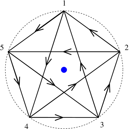
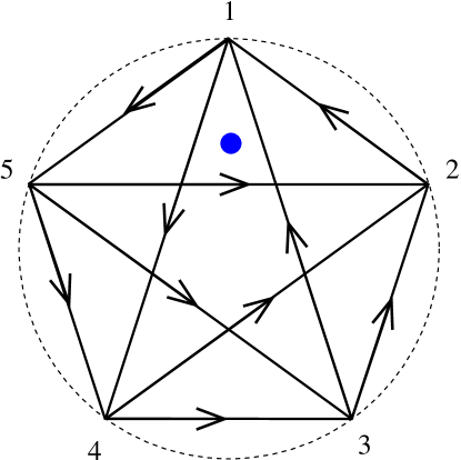
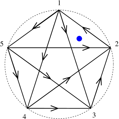
An interesting subset of well split quivers satisfies a different pictorial constraint. Instead of checking each node individually that all the incoming arrows come from the right in the collection and all the outgoing arrows go to the left, one searches the quiver for a polygon such that around the polygon, all the arrows travel counterclockwise. Note that the quiver may have to be deformed to get the polygon to appear.

Figure 1 shows the three types of well split five node quivers that typically appear. (Note there are also degenerate cases where some arrows are missing.) The three types correspond to the three types of polygons in this geometric construction.

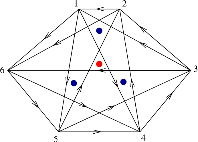
The existence of such a polygon clearly implies well split. Put a point inside the polygon. Pick any node. Join the point and the node with a line. All the arrows incident on this node to one side of this line will be ingoing while all the arrows on the other side will be outgoing. That well split implies the existence of such a polygon is not trivial, and we leave it as a conjecture. Figure 2 provides an apparent counterexample. However, we can deform the quiver such that the triangle with a red dot disappears and a new triangle appears with the required counterclockwise property.

Figure 2: A well split six node quiver. The blue dots label polygons around which only nearby arrows travel counterclockwise. The red dot labels a triangle which can disappear if the nodes are moved. Indeed, if we move nodes 1 and 2 farther apart and 4 and 5 closer together, the triangle with a red dot will disappear and a new triangle will take its place around which all arrows travel counterclockwise.

Exploring the value of our sheaf theoretic definition of Seiberg duality, we are also led to wonder if we can take arbitrary Seiberg duals of Seiberg duals. For that we would need the following.

Conjecture 1 (Section 5 of [13]).

The Seiberg dual of a well split quiver is well split.

The conjecture is trivial for three node exceptional quivers and was proved for the four node exceptional quivers in [13]. In the following, we will prove what superficially appears to be a weaker version of this conjecture. However, we are uncertain that a stronger version exists.

Our two principal results are

Theorem 5.3.

A strong helix $\mathcal{H}$ generates a well split quiver.

and

Theorem 5.4.

Let $\mathcal{H}$ be a strong helix. Let $\mathcal{E}$ be a foundation of $\mathcal{H}$. The Seiberg dual $\mathcal{E}^{\prime}$ of $\mathcal{E}$ generates a strong helix $\mathcal{H}^{\prime}$.

5.1 Proof of Theorem 5.3

To prove Theorem 5.3, we introduce an intermediate notion, $\mbox{Ext}^{1,2}$. We will prove that $\mbox{Ext}^{1,2}$ implies well split and then finish by demonstrating that $\mbox{Ext}^{1,2}$ is equivalent to the strong helix property.

In this paper, we are concerned with $\mathcal{E}$ constructed from del Pezzo surfaces. We see from (22) that the object $E_{n}^{\vee}\in\mathcal{E}^{Q}$ considered as a sheaf will have a shift of grading equal to two. Meanwhile, the object $E_{1}^{\vee}=\delta E_{1}$ is not shifted at all. Because the shifts of grading can only increase as we left mutate $E_{i}$, the non-zero sheaf in the complex $E_{i}^{\vee}$ can be shifted only zero, one, or two places. We imagine the following nice scenario where

$$\mathcal{E}^{Q} = (E_{n}^{\vee},\ldots,E_{1}^{\vee})$$ (38)

$$= (\delta F_{n}[2],\ldots,\delta F_{b}[2],\delta F_{b-1}[1],\ldots,\delta F_{c}[1],\delta F_{c-1},\ldots,\delta F_{1})$$

and the $F_{i}$ are sheaves. Clearly the $\mathbb{P}^{2}$ example satisfies this condition. Indeed all three block exceptional collections in [32] also satisfy this condition, and examples are known for all del Pezzos. We assume the preceding blocking structure for $\mathcal{E}^{Q}$ and also that $\mbox{Hom}^{k}(E_{i}^{\vee},E_{j}^{\vee})=0$ unless $k=1$ or 2. We will call these two conditions together the $\mbox{Ext}^{1,2}$ condition. In the preceding sections, we spent a substantial amount of time explaining the second condition using physics considerations.

Lemma 5.5.

The $\mbox{Ext}^{1,2}$ condition implies well split.

Proof.

Consider two sheaves $F_{i}$ and $F_{j}$ in $\mathcal{E}^{Q}$ with the same grading, $i>j$. Either $\mbox{Hom}(F_{i},F_{j})=0$ or $\mbox{Ext}^{1}(F_{i},F_{j})=0$ because $(F_{i},F_{j})$ form an exceptional pair. However, to satisfy the $\mbox{Ext}^{1,2}$ condition, we must have $\mbox{Hom}(F_{i},F_{j})=0$. Thus, the arrow in the quiver points from $i$ to $j$. We conclude there can be no violations of the well split condition within a block of sheaves of the same grading.

We can conclude slightly more from the preceding. In particular, recall that $\chi_{-}(F_{i},F_{j})=\chi(F_{i},F_{j})$. Thus, the slopes must satisfy $\mu(F_{i})\geq\mu(F_{j})$.

Next consider $\delta F_{i}[2]$ and $\delta F_{j}$ for $n\geq i\geq b$ and $c-1\geq j\geq 1$. By the $\mbox{Ext}^{1,2}$ condition, $\mbox{Ext}^{1}(F_{i},F_{j})=0$ or we would have an $\mbox{Hom}^{3}$ type map in $D^{\flat}(\mathcal{B})$. Thus, the arrow, if it exists, points from $j$ to $i$.

The only possible violation to well split will occur for maps between sheaves with gradings shifted by one. Consider $\delta F_{i}[2]$ for $n\geq i\geq b$ and $\delta F_{j}[1]$, $\delta F_{k}[1]$ for $b-1\geq j>k\geq c$. Assume $\mbox{Ext}^{1}(F_{i},F_{j})\neq 0$, i.e. there is an arrow from $j$ to $i$. We would have a violation of well split if then $\mbox{Hom}(F_{i},F_{k})\neq 0$, but such a violation cannot occur for the following reason. $\mbox{Ext}^{1}(F_{i},F_{j})\neq 0$ implies that $\mu(F_{j})<\mu(F_{i})$. We have from the first part of the proof that $\mu(F_{j})\geq\mu(F_{k})$. Therefore $\mu(F_{k})<\mu(F_{i})$ and the map from $F_{i}$ to $F_{k}$ must also be of type $\mbox{Ext}^{1}$. A similar argument rules out violations of the well split condition for maps from $F_{i}[1]$ to $F_{j}$ in $\mathcal{E}^{Q}$. ∎

We also have a useful corollary for the values of the slopes.

Corollary 5.6.

For a collection $\mathcal{E}^{Q}$ satisfying the $\mbox{Ext}^{1,2}$ condition, the slopes of the sheaves with a given grading are in descending order within $\mathcal{E}^{Q}$. In particular, for $n\geq i>j\geq b$ or for $b-1\geq i>j\geq c$ or for $c-1\geq i>j\geq 1$, $\mu(F_{i})\geq\mu(F_{j})$. Moreover, $\mu(F_{n})\leq\mu(F_{1})$.

Given an $\mathcal{E}^{Q}$, we are assuming that $\mathcal{E}^{Q}$ was constructed from a collection $\mathcal{E}$ where all the sheaves in $\mathcal{E}$ are torsion free. Otherwise, the corresponding gauge groups would have rank zero, and we would lose our physical motivation for studying these collections. It may be that $\mathcal{E}^{Q}$ is also torsion free, but we have not been able to prove it, and it is therefore worthwhile to consider the special cases where some of the $E_{i}^{\vee}$ have zero rank.

Our proof of Lemma 5.5 holds whether or not some of the $E_{i}^{\vee}$ are torsion. If $F_{i}$ were torsion, we take $\mu(F_{i})=\infty$ and $\mu(F_{i})\geq\mu(F_{j})$ $\forall j$.

Interestingly, the torsion sheaves can only occur in special places inside $\mathcal{E}^{Q}$.

Remark 5.7.

If $F_{i}$ is torsion then $i=b-1$ or $i=c-1$ or $F_{i+1}$ is torsion.

Because $F_{n}=E_{n}\otimes K$ is not torsion, the torsion sheaves will only appear in (38) shifted by zero or one.

The $\mbox{Ext}^{1,2}$ property strongly constrains the form of the original collection $\mathcal{E}$. To see these constraints, we need the following lemma.

Lemma 5.8.

The chern character of $E_{j}^{\vee}$ is

$$\mbox{ch}(E_{j}^{\vee})=\sum_{i=1}^{j}S_{ij}\mbox{ch}(E_{i})\ .$$ (39)

Proof.

From the definition of $S$,

$$\chi(E_{j}^{\vee},E_{i}^{\vee})=S_{ij}\ .$$ (40)

From (26),

$$\chi(E_{i},E_{j}^{\vee})=\delta_{ij}\ .$$ (41)

Because $\mathcal{E}$ is complete, we can express the chern character of any sheaf as a sum over the chern characters of the $E_{i}\in\mathcal{E}$. In particular

$$\mbox{ch}(E_{j}^{\vee})=\sum_{i}a_{ij}\mbox{ch}(E_{i})\ .$$ (42)

The lemma follows from acting on each side of the equality with $\chi(\cdot,E_{k}^{\vee})$. ∎

Corollary 5.9.

Since $S$ has an inverse, we find

$$\mbox{ch}(E_{j})=\sum_{i=1}^{j}S_{ij}^{-1}\mbox{ch}(E_{i}^{\vee})\ .$$ (43)

Proposition 5.10.

If $\mathcal{E}^{Q}$ is $\mbox{Ext}^{1,2}$, then the original collection $\mathcal{E}$ generates a strong helix.

Proof.

Using Corollary 5.9, we have

$$\mu(E_{j-1}) \leq \mu(E_{j})\Leftrightarrow$$

$$\frac{\sum_{i=1}^{j-1}\mbox{deg}(E_{i}^{\vee})S^{-1}_{i(j-1)}}{\sum_{i=1}^{j-1}r(E_{i}^{\vee})S^{-1}_{i(j-1)}} \leq \frac{\sum_{i=1}^{j}\mbox{deg}(E_{i}^{\vee})S^{-1}_{ij}}{\sum_{i=1}^{j}r(E_{i}^{\vee})S^{-1}_{ij}}\ .$$

Note that by assumption, all the ranks of the sheaves in $\mathcal{E}$ are positive. We can clear the denominators without flipping the sign of the inequality. Thus

$$\mu(E_{j-1}) \leq \mu(E_{j})\Leftrightarrow$$

$$\sum_{i=1}^{j-1}\sum_{k=1}^{j}S_{i(j-1)}^{-1}S_{kj}^{-1}(\mbox{deg}(E_{i}^{\vee})r(E_{k}^{\vee})-\mbox{deg}(E_{k}^{\vee})r(E_{i}^{\vee})) \leq 0\Leftrightarrow$$

$$\sum_{i=1}^{j-1}\sum_{k=1}^{j}S_{i(j-1)}^{-1}S_{kj}^{-1}(S_{ik}-S_{ki}) \leq 0\Leftrightarrow$$

$$-S_{(j-1)j}^{-1} \leq 0\ .$$

The fact that $S$ is upper triangular and has ones on the diagonal implies that $S_{(j-1)j}^{-1}=-S_{(j-1)j}$. Moreover, well split tells us that $S_{(j-1)j}\leq 0$.

From Corollary 5.6, we have that $\mu(F_{n})\leq\mu(F_{1})$. Note that $F_{n}=E_{n}\otimes K$ and $F_{1}=E_{1}$. Thus, $\mu(E_{n})-K^{2}\leq\mu(E_{1})$ and the helix must be strongly exceptional. ∎

Proposition 5.11.

If $\mathcal{E}$ generates a strong helix, then $\mathcal{E}^{Q}$ is $\mbox{Ext}^{1,2}$.

We will spend the rest of this section in a rather technical proof of this important proposition. The strategy is first to show that $\mathcal{E}^{Q}$ respects the blocking structure of grading shifts in the definition of $\mbox{Ext}^{1,2}$. Next, we will demonstrate that the slopes satisfy Corollary 5.6.

Claim 5.12.

By the braid group relations,

$$\delta E_{j}=R_{E_{1}^{\vee}}^{D}\cdots R_{E_{j-1}^{\vee}}^{D}E_{j}^{\vee}\ .$$ (44)

Inverting this relation, we find

$$E_{j}^{\vee}=L_{E_{j-1}^{\vee}}^{D}\cdots L_{E_{1}^{\vee}}^{D}\delta E_{j}\ .$$ (45)

The chern character of $E_{j}^{\vee}$ can then be expanded as

$$\mbox{ch}(E_{j}^{\vee}) = \mbox{ch}(E_{j})-\sum_{i=1}^{j-1}\chi(E_{i}^{\vee},L_{E_{i-1}^{\vee}}^{D}\cdots L_{E_{1}^{\vee}}^{D}E_{j})\mbox{ch}(E_{i}^{\vee})$$

$$= \mbox{ch}(E_{j})-\sum_{i=1}^{j-1}\chi(E_{i},E_{j})\mbox{ch}(E_{i}^{\vee})$$

$$= \mbox{ch}(E_{j})-\sum_{i=1}^{j-1}S_{ij}^{-1}\mbox{ch}(E_{i}^{\vee})\ ,$$

which agrees with the result of Corollary 5.9. We have rederived this result to see that each term in the sum corresponds to a separate left mutation and thus a separate opportunity for the complex $E_{j}^{\vee}$ to be shifted by one with respect to $\delta F_{j}$. Note that

$$r(E_{j}^{\vee})=r(E_{j})\left[1-\sum_{i=1}^{j-1}r(E_{i})r(E_{i}^{\vee})(\mu_{j}-\mu_{i})\right]\ .$$ (46)

As we sum from $i=1$ to $j-1$, each time the term in brackets changes sign, $E_{j}^{\vee}$ will shift by one with respect to $\delta F_{j}$. Note that if a partial sum is zero, there is no corresponding shift in grading because for left mutations a torsion sheaf can only be produced by a recoil, and there is no shift in grading for a recoil.

Let $c$ be the smallest integer such that $r(E_{c}^{\vee})<0$. There must exist such a $c$ because $E_{n}^{\vee}$ is shifted by two with respect to $\delta F_{n}$. For all $i<c$, there is no relative shift and $E_{i}^{\vee}=\delta F_{i}$. We now argue that for all $i>c$, $E_{i}^{\vee}=\delta F_{i}[s_{i}]$ where $s_{i}$ is either one or two. The reason is that $\mathcal{E}$ is strongly exceptional and $\mu_{i}\leq\mu_{i+1}$. In particular,

$$\sum_{i=1}^{c-1}r(E_{i})r(E_{i}^{\vee})(\mu_{c}-\mu_{i})\leq\sum_{i=1}^{c-1}r(E_{i})r(E_{i}^{\vee})(\mu_{k}-\mu_{i})$$ (47)

for $k>c$. Thus, $E_{k}^{\vee}$ will be shifted by at least one with respect to $\delta F_{k}$. To summarize, we have found that

$$\mathcal{E}^{Q}=(\delta F_{n}[s_{n}],\ldots,\delta F_{c+1}[s_{c+1}],\delta F_{c}[1],\delta F_{c-1},\ldots,\delta F_{1})\ .$$ (48)

where $s_{i}=1$ or 2.

We now take advantage of the helix structure to complete a proof of the fact that $\mathcal{E}^{Q}$ contains objects with the appropriate shifts of grading. Using

$$\delta E_{i}\otimes K[2]=L_{\delta E_{i+1}\otimes K[2]}^{D}\cdots L_{\delta E_{n}\otimes K[2]}^{D}L_{\delta E_{1}}^{D}\cdots L_{\delta E_{i-1}}^{D}\delta E_{i}\ ,$$ (49)

we find that

$$E_{i}^{\vee}=R_{\delta E_{n}\otimes K[2]}^{D}\cdots R_{\delta E_{i+1}\otimes K[2]}^{D}(\delta E_{i}\otimes K[2])\ .$$ (50)

With the braid relations,

$$\delta E_{i}\otimes K[2]=L_{E_{n}^{\vee}}^{D}\cdots L_{E_{i+1}^{\vee}}^{D}E_{i}^{\vee}\ ,$$ (51)

and thus

$$E_{i}^{\vee}=R_{E_{i+1}^{\vee}}^{D}\cdots R_{E_{n}^{\vee}}^{D}(\delta E_{i}\otimes K[2])\ .$$ (52)

Just as done above, we can use this expression for $E_{i}^{\vee}$ to derive a relation on $\mbox{ch}(E_{i}^{\vee})$:

$$\mbox{ch}(E_{j}^{\vee})=\mbox{ch}(E_{j}\otimes K)-\sum_{i=j+1}^{n}S_{ij}^{-1}\mbox{ch}(E_{j}^{\vee})\ .$$ (53)

For the ranks, we find then

$$r(E_{j}^{\vee})=r(E_{j})\left[1-\sum_{i=j+1}^{n}r(E_{i})r(E_{i}^{\vee})(\mu_{i}-\mu_{j})\right]$$ (54)

which could have been derived from (5.9) and chiral anomaly cancellation ($(S-S^{T})\cdot r=0$), but now again we have an interpretation of each term in the sum in brackets as a right mutation.

As before, we find that there is a $b$ such that $r(E_{i}^{\vee})>0$ for $n\geq i\geq b$ and $r(E_{b-1}^{\vee})\leq 0$. Moreover, for $i<b$, $E_{i}^{\vee}=\delta F_{i}[s_{i}]$ and $s_{i}$ is either zero or one. In particular

$$\mathcal{E}^{Q}=(\delta F_{n}[2],\ldots,\delta F_{b}[2],\delta F_{b-1}[1],\delta F_{b-2}[s_{b-2}]\ldots\delta F_{1}[s_{1}])\ .$$ (55)

Putting (48) and (55) together, we conclude that the shifts of grading of $\mathcal{E}^{Q}$ are precisely as in (38).

The last remaining step in the proof of Theorem 5.3 is to check that the slopes are as in Corollary 5.6 (which in turn implies the restriction on the types of Ext maps between the sheaves). We first consider the $E_{i}^{\vee}$ which are torsion free. Notice that $\mbox{sign}(r(E_{i}^{\vee}))=\mbox{sign}(r(E_{j}^{\vee}))$ for $n\geq i>j\geq b$ or for $b-1\geq i>j\geq c$ or for $c-1\geq i>j\geq 1$. Using Lemma 5.8, we have

$$\mu(E^{\vee}_{j-1}) \leq \mu(E^{\vee}_{j})\Leftrightarrow$$

$$\frac{\sum_{i=1}^{j-1}\mbox{deg}(E_{i})S_{i(j-1)}}{\sum_{i=1}^{j-1}r(E_{i})S_{i(j-1)}} \leq \frac{\sum_{i=1}^{j}\mbox{deg}(E_{i})S_{ij}}{\sum_{i=1}^{j}r(E_{i})S_{ij}}\ .$$

We can clear the denominators without flipping the sign of the inequality only if $\mbox{sign}(r(E_{j-1}^{\vee}))=\mbox{sign}(r(E_{j}^{\vee}))$, which will be true if $E_{j}^{\vee}$ and $E_{j-1}^{\vee}$ are shifted by the same amount. Manipulations analogous to those in the proof of Proposition 5.10 show

$$\mu(E^{\vee}_{j-1}) \leq \mu(E^{\vee}_{j})\Leftrightarrow$$

$$\sum_{i=1}^{j-1}\sum_{k=1}^{j}S_{i(j-1)}S_{kj}(\mbox{deg}(E_{i})r(E_{k})-\mbox{deg}(E_{k})r(E_{i})) \leq 0\Leftrightarrow$$

$$\sum_{i=1}^{j-1}\sum_{k=1}^{j}S_{i(j-1)}S_{kj}(S_{ki}^{-1}-S_{ik}^{-1}) \leq 0\Leftrightarrow$$

$$S_{(j-1)j} \leq 0\ .$$

From the structure of these upper triangular matrices, $S_{(j-1)j}=-S_{(j-1)j}^{-1}$. From the strong exceptional property, $S_{(j-1)j}^{-1}\geq 0$.

We also check that $\mu(F_{n})\leq\mu(F_{1})$. Note that $\mu(F_{n})=\mu(E_{n}\otimes K)=\mu(E_{n})-K^{2}$ and $\mu(F_{1})=\mu(E_{1})$. But we know that $\mu(E_{n})\leq\mu(E_{1})+K^{2}$ because $\mathcal{E}$ generates a strong helix.

Finally, we consider the $E_{i}^{\vee}$ which are torsion. If the torsion sheaves occur as in Remark 5.7, then $\mathcal{E}^{Q}$ continues to satisfy the conditions of Corollary 5.6 because the slope of a torsion sheaf is infinite. Note that $F_{1}=E_{1}$ and $F_{n}=E_{n}\otimes K$ are torsion free from our assumption about $\mathcal{E}$. We can then finish our proof of Proposition 5.11 by showing that for $E_{i}^{\vee}$ and $E_{i+1}^{\vee}$ shifted by the same amount, if $F_{i}$ is torsion, then so is $F_{i+1}$:

$$S_{i(i+1)}=\chi(E_{i+1}^{\vee},E_{i}^{\vee})=\chi(F_{i+1},F_{i})=r(F_{i+1})\geq 0\ .$$

However, as above we have that $S_{i(i+1)}=-S^{-1}_{i(i+1)}\leq 0$ and we conclude that $r(F_{i+1})=0$.

5.2 Proof of Theorem 5.4

Let $\mathcal{E}$ generate a strong helix. We are free to take the Seiberg dual of $E_{n}$ without loss of generality. (We just choose an appropriate foundation of the helix. The strong property of the helix means that any foundation will also be strongly exceptional.) Let $\mathcal{E}^{\prime}$ be the Seiberg dual collection:

$$\mathcal{E}^{\prime}=(E_{1},\ldots,E_{a},L_{E_{a+1}}\cdots L_{E_{n-1}}E_{n},E_{a+1},\ldots,E_{n-1})$$ (56)

where we have assumed that nodes 1 through $a$ all have arrows ending on node $n$ while nodes $a+1$ through $n-1$ have arrows beginning at node $n$. Note that from the helix property,

$$E_{n}^{\prime}\equiv L_{E_{a+1}}\cdots L_{E_{n-1}}E_{n}=R_{E_{1}}\cdots R_{E_{a}}(E_{n}\otimes K)\ .$$ (57)

Our strategy is to show that the slopes of $\mathcal{E}^{\prime}$ satisfy the conditions of Remark 3.10. $\mathcal{E}^{\prime}$ is an exceptional collection, and the conditions on the slopes are sufficient to guarantee that $\mathcal{E}^{\prime}$ is strongly exceptional and in fact generates a strong helix.

Lemma 5.13.

The chern character of $E_{n}^{\prime}$ is

$$\mbox{ch}(E_{n}^{\prime})=-\sum_{i=a+1}^{n}S_{in}\mbox{ch}(E_{i})\ .$$ (58)

Proof.

From the definition of mutation in terms of short exact sequences, we find that

$$\mbox{ch}(E_{n}^{\prime})=(-1)^{\delta_{n-1}}\mbox{ch}(E_{n})+\sum_{i=a+1}^{n-1}(-1)^{\delta_{i}}S_{in}^{\prime}\mbox{ch}(E_{i})\$$ (59)

where we have defined

$$S_{in}^{\prime}=-\chi(E_{i},L_{E_{i+1}}\cdots L_{E_{n-1}}E_{n})\$$ (60)

and $\delta_{i}$ is the number of mutations among the $L_{E_{a+1}},\ldots,L_{E_{i}}$ of type division.

Recall the definition

$$S_{jn}=\chi(E_{n}^{\vee},E_{j}^{\vee})=(L_{\delta E_{1}}^{D}\cdots L_{\delta E_{n-1}}^{D}\delta E_{n},L_{\delta E_{1}}^{D}\cdots L_{\delta E_{j-1}}^{D}\delta E_{j})\ .$$ (61)

We can massage this formula into something a little more useful

$$S_{jn} = \chi(L_{\delta E_{j}}^{D}\cdots L_{\delta E_{n-1}}^{D}\delta E_{n},\delta E_{j})$$

$$= -\chi(\delta E_{j},L_{\delta E_{j+1}}^{D}\cdots L^{D}_{\delta E_{n-1}}\delta E_{n})$$

$$= (-1)^{\epsilon_{j}}S_{jn}^{\prime}$$

where $\epsilon_{i}$ is number of mutations of type division among the $L_{E_{i+1}},\ldots,L_{E_{n-1}}$. Clearly, $\epsilon_{i}+\delta_{i}$ is a constant. In particular, $\epsilon_{i}+\delta_{i}=\epsilon_{a}=\delta_{n-1}$. We conclude that

$$\mbox{ch}(E_{n}^{\prime})=(-1)^{\epsilon_{a}}\left[\mbox{ch}(E_{n})+\sum_{i=a+1}^{n-1}S_{1i}\mbox{ch}(E_{i})\right]\ .$$ (62)

We argue that $\epsilon_{a}=1$. $\epsilon_{a}=0$, $1$, or $2$ and, from (22), there would be exactly two divisions if we were to left mutate $E_{n}$ through the whole collection. For an exceptional pair $(F,E)$, recall that a division occurs whenever $r(L^{D}_{\delta F}\delta E)=r(E)-\chi(E,F)r(F)$ is negative. The well split condition implies that $S_{in}\geq 0$ for $1\leq i\leq a$ and $S_{in}\leq 0$ for $a+1\leq i\leq n-1$. In order to have two divisions as a result of mutating $E_{n}$ through the collection, from the signs of the $S_{in}$, we need exactly one division by the time we get to $i=a+1$. Therefore $\epsilon_{a}=1$. ∎

Note that $r(E_{n}^{\prime})>0$ and $E_{n}^{\prime}$ cannot be torsion because the grading does not shift if a left mutation produces a torsion sheaf.

It follows from Lemma 5.13 that the slope of $E_{n}^{\prime}$ is

$$\mu(E_{n}^{\prime})=\frac{\mbox{deg}(E_{n}^{\prime})}{r(E_{n}^{\prime})}=\frac{-\sum_{i=a+1}^{n}S_{in}\mbox{deg}(E_{i})}{-\sum_{i=a+1}^{n}S_{in}r(E_{i})}\ .$$ (63)

Lemma 5.14.

The slope of $E_{n}^{\prime}$ satisfies the inequality:

$$\mu(E_{n}^{\prime})\geq\mu(E_{a})\ .$$ (64)

Proof.

$$\mu(E_{n}^{\prime}) \geq \mu(E_{a})\Leftrightarrow$$

$$\sum_{i=a+1}^{n}S_{in}\left(r(E_{i})\mbox{deg}(E_{a})-r(E_{a})\mbox{deg}(E_{i})\right) \geq 0\Leftrightarrow$$

$$-\sum_{i=a+1}^{n}S_{ai}^{-1}S_{in} \geq 0\Leftrightarrow$$

$$S_{an} \geq 0\ .$$ (65)

By the well split assumption, $S_{an}\geq 0$. ∎

Lemma 5.15.

The slope of $E_{n}^{\prime}$ satisfies the additional inequality:

$$\mu(E_{n}^{\prime})\leq\mu(E_{a+1})\ .$$ (66)

Proof.

It is convenient to choose a different foundation for the helix to check the inequality. We rename $E_{n}\otimes K=E_{0}$, and then we introduce

$$\mathcal{F}=(F_{1},\ldots,F_{n})=(E_{0},E_{1},\ldots,E_{n-1})\ .$$ (67)

Using (57) and an argument analogous to the proof of Lemma 5.13, we find that

$$\mbox{ch}(E_{n}^{\prime})=-\sum_{i=1}^{a+1}S_{1i}\mbox{ch}(F_{i})\$$ (68)

where now the $S_{ij}$ have been defined with respect to $\mathcal{F}$. It follows that

$$\mu(E_{n}^{\prime})=\frac{-\sum_{i=1}^{a+1}S_{1i}\mbox{deg}(F_{i})}{-\sum_{i=1}^{a+1}S_{1i}r(F_{i})}\ .$$ (69)

One additional subtlety is the fact that we are using right mutations to construct $E_{n}^{\prime}$. Thus we need the fact from the proof of Lemma 5.13 that $r(E_{n}^{\prime})\neq 0$. An argument equivalent to (65) demonstrates that $\mu(E_{n}^{\prime})\leq\mu(F_{a+2})=\mu(E_{a+1})$ if and only if $S_{1(a+2)}\geq 0$, which follows from well split. ∎

From Lemmas 5.14 and 5.15, it follows that $\mathcal{E}^{\prime}$ is strongly exceptional.

Now we check that $\mathcal{E}^{\prime}$ generates a strong helix. Note that $\mu(E_{n})-K^{2}\leq\mu(E_{1})\leq\mu(E_{2})$ so $\mu(E_{n})-K^{2}\leq\mu(E_{2})$.

6 Recovering the Old Seiberg Duality

As promised, we discuss how our definition of Seiberg duality matches the original definition.

For the original Seiberg duality, one takes a node $i$ of a supersymmetric quiver and reverses the orientation of all the arrows incident on that node, $X_{ij}\to X_{ji}^{\prime}$ and $Y_{ji}\to Y_{ij}^{\prime}$. The old maps $X_{ij}$ and $Y_{ki}$ one combines to make so called mesonic fields (or maps) $M_{kj}=X_{ij}Y_{ki}$. To the superpotential, one adds new mass terms $W\to W+M_{kj}Y_{ik}^{\prime}X_{ji}^{\prime}$ for each $M_{kj}$ field.

Sometimes, the $M_{kj}$ maps will be oriented opposite to the maps $X_{kj}$ or $X_{jk}$ present in the original quiver. If we hope to be able to represent the quiver with exceptional collections, we need to be able to ensure that the maps between $k$ and $j$ are only in one direction. One can “integrate out” the $M_{kj}$ (or equivalently the $X_{jk}$), by which is meant one uses the relations $\partial W/\partial M_{kj}=0$ to eliminate $M_{kj}$ from W. Such a procedure is not always possible.

Let’s compare this procedure with exceptional collections. We Seiberg dualize on node 1, obtaining the collection $\mathcal{E}^{\prime}$ given by

$$\mathcal{E}^{\prime}=(E_{2},\ldots,E_{a},R_{E_{a}}\cdots R_{E_{2}}E_{1},E_{a+1},\ldots,E_{n})$$ (70)

Proposition 6.1.

The dual exceptional collection ${\mathcal{E}^{Q}}^{\prime}$ takes the form

$${\mathcal{E}^{Q}}^{\prime}=(E_{n}^{\vee},\ldots,E_{a+1}^{\vee},\delta E_{1}[1],R_{\delta E_{1}}^{D}E_{a}^{\vee},\ldots,R_{\delta E_{1}}^{D}E_{2}^{\vee})\ .$$ (71)

Proof.

The result follows from the expression for $\mathcal{E}^{\prime}$ (70), the definition of $\mathcal{E}^{Q}$ (25), and the braid group relations (20). ∎

From this Proposition, we see that the complex $\delta E_{1}$ corresponding to the dualized node gets shifted by one under Seiberg duality, reversing the orientation of all the arrows incident on node $1$. Moreover, the number of arrows from $k$ to $j$ is shifted by

$$S_{kj}\to\chi(E_{j}^{\vee},R^{D}_{\delta E_{1}}E_{k}^{\vee})=S_{kj}-S_{1k}S_{1j}$$ (72)

If $S_{kj}>0$, the number of arrows between $k$ and $j$ matches the original definition of Seiberg duality. If $S_{kj}<0$, we have to assume in the original picture of Seiberg duality that we can integrate out enough of the $M_{kj}$ or $X_{jk}$ such that the result has maps only in one direction.

The original definition of Seiberg duality also came with an induced action on the quiver representation, often denoted by physicists as $N_{c}\to N_{f}-N_{c}$ where $N_{c}$, the number of colors, is the rank $d^{i}$ of the vector space at the dualized node $i$ and $N_{f}$ is the number of flavors. In particular, if we were to dualize node 1 say,

$$N_{f}=-\sum_{i=2}^{a}S_{1i}d^{i}\ .$$ (73)

In other words, we recover

$$d^{1}\to-\sum_{i=1}^{a}S_{1i}d^{i}$$ (74)

in agreement with Lemma 5.13.

7 Discussion

The results in this paper help to resolve a number of bothersome puzzles and raise some interesting questions. As we discuss presently, these puzzles concern 1) the recipe for constructing a gauge theory from an exceptional collection, 2) negative conformal dimensions of gauge invariant operators, 3) the connection between the exceptional collection literature in mathematics and del Pezzo gauge theories in physics, and 4) the connection between different mathematical formulations of Seiberg duality.

The original recipe for writing down a gauge theory quiver from an exceptional collection presented in section 4 now makes a lot more sense if we assume the collection generates a strong helix. The original recipe for writing down a gauge theory quiver from an exceptional collection relied only on the sign of the Euler character, seeming to ignore the significance of whether the maps between the sheaves were of type $\mbox{Ext}^{0}$, $\mbox{Ext}^{1}$, $\mbox{Ext}^{2}$, or $\mbox{Ext}^{3}$. From the discussion in section 2, we expected that only $\mbox{Hom}_{D^{\flat}(\mathbf{X})}^{1}(E,F)$ type maps should correspond to bifundamental fields in the gauge theory. If the collection generates a strong helix, we find that there will only be $\mbox{Hom}_{D^{\flat}(\mathbf{X})}^{1}$ type maps and the sign of the Euler character just lets us know whether the map descended from a $\mbox{Hom}^{1}_{D^{\flat}(\mathcal{B})}$ or $\mbox{Hom}^{2}_{D^{\flat}(\mathcal{B})}$ in the del Pezzo.

The recipe makes more sense not only in a physics context but also a mathematical one. We can think about the gauge theory quiver as generating an algebra, the path algebra of the quiver. This path algebra is nothing but the maps between the sheaves in the helix $\mathcal{H}$, at least as long as $\mathcal{H}$ is a strong helix. However, if there are higher Ext maps between the sheaves in $\mathcal{H}$, it is far less clear to what this path algebra of the quiver corresponds.

Concerns have been raised in the literature [13] about possible gauge invariant, chiral operators with negative R-charge (and hence negative conformal dimension) which our results here eliminate. The authors of [26], inspired in particular by work of [34] but also by [35], give a formula for the R-charges of the bifundamental fields $X_{ij}$. If $i<j$, then either

$$\frac{K^{2}}{2}R(X_{ij})=\mu_{j}-\mu_{i}$$ (75)

or

$$\frac{K^{2}}{2}R(X_{ji})=K^{2}-\mu_{j}+\mu_{i}\ ,$$ (76)

depending on whether the arrow goes from $i$ to $j$ or from $j$ to $i$. For general exceptional collections, $R(X_{ij})$ may be less than zero. While not of concern by itself, gauge invariant combinations of the these $X_{ij}$, called dibaryon operators, can be made which also have negative R-charge. However, for strong helices

$$0\leq\mu_{j}-\mu_{i}\leq K^{2}$$ (77)

and hence the R-charges will always be positive.

Our results demonstrate the physical relevance of certain mathematical concepts and we hope may serve as inspiration to those who study exceptional collections for their own sake. Unaware of the connection to gauge theory, Bondal [21] defined and studied strong helices and admissible mutations. For example, Corollary 7.3 of [21] states that if $\mathcal{E}^{Q}$ is strongly exceptional and Koszul, then $\mathcal{E}$ is strongly exceptional. In this paper, we have replaced Corollary 7.3 with an equivalence between $\mbox{Ext}^{1,2}$ and strong helices. Section 8 of [21] is a preliminary investigation of admissible mutations of strong helices. Here, we have been able to argue that an important class of these admissible mutations are Seiberg dualities. The precise connection between Koszul and $\mbox{Ext}^{1,2}$ and whether or not there are other admissible mutations in addition to Seiberg dualities deserve further thought.

These admissible mutations of strongly exceptional collections must be closely related to the tilting equivalences of Berenstein and Douglas [14]. Bondal [21] constructs a quiver from strongly exceptional collections. The quiver he constructs, the Beilinson quiver of section 4, is not quite the gauge theory quiver but is closely related to it. He is then able to prove (Theorem 6.2 of [21]) that for strongly exceptional collections, $D^{\flat}(\mathcal{B})$ is equivalent to the derived category constructed from the quiver. We suspect there must be a stronger theorem which relates the derived category constructed from the gauge theory quiver to $D^{\flat}(\mathbf{X})$ and that in this context tilting equivalences will prove to be precisely admissible mutations.

There are at least two important physics questions that we have not been able to address here. One is the existence of an analog of the orbifold point in the Kaehler moduli space of $\mathbf{X}$ where all the D-branes become mutually supersymmetric. Without such a point or locus, our gauge theory construction fails. We think it likely such a point exists, but there are no guarantees, and a more careful analysis of the Kaehler moduli space of these del Pezzos is in order. Two is whether anything we have learned here about strongly exceptional collections can be applied to the other physical situations where exceptional collections are important, for example the Landau-Ginzburg models of [22, 23]. We leave these questions for the future.

Note added: After the electronic distribution of the first version of this work, [36] appeared which has some overlap with our results.

Acknowledgments

I would like to thank Paul Aspinwall, Brian Conrad, Igor Dolgachev, and David Gross, for useful conversations. I would also especially like to thank David Berenstein, James McKernan, and Johannes Walcher for comments on the manuscript. Finally, I am grateful to the referee for insisting on a more careful treatment of torsion sheaves. This research was supported in part by the National Science Foundation under Grant No. PHY99-07949.

References

- [1] A. Hanany and J. Walcher, “On duality walls in string theory,” JHEP 0306, 055 (2003) [arXiv:hep-th/0301231].
- [2] S. Franco, A. Hanany, Y. H. He and P. Kazakopoulos, “Duality walls, duality trees and fractional branes,” arXiv:hep-th/0306092.
- [3] S. Franco, Y. H. He, C. Herzog and J. Walcher, “Chaotic duality in string theory,” arXiv:hep-th/0402120.
- [4] I. R. Klebanov and M. J. Strassler, “Supergravity and a confining gauge theory: Duality cascades and chiSB-resolution of naked singularities,” JHEP 0008, 052 (2000) [arXiv:hep-th/0007191].
- [5] N. Seiberg, “Electric - magnetic duality in supersymmetric nonAbelian gauge theories,” Nucl. Phys. B 435, 129 (1995) [arXiv:hep-th/9411149].
- [6] K. A. Intriligator and N. Seiberg, “Lectures on supersymmetric gauge theories and electric-magnetic duality,” Nucl. Phys. Proc. Suppl. 45BC, 1 (1996) [arXiv:hep-th/9509066].
- [7] C. E. Beasley and M. Ronen Plesser, “Toric Duality is Seiberg Duality,” JHEP 0112 (2001) 001, [arXiv:hep-th/0109053].
- [8] B. Feng, A. Hanany, Y. H. He and A. M. Uranga, “Toric duality as Seiberg duality and brane diamonds,” JHEP 0112, 035 (2001) [arXiv:hep-th/0109063].
- [9] F. Cachazo, B. Fiol, K. A. Intriligator, S. Katz and C. Vafa, “A geometric unification of dualities,” Nucl. Phys. B 628, 3 (2002) [arXiv:hep-th/0110028].
- [10] H. Ooguri and C. Vafa, “Geometry of N = 1 dualities in four dimensions,” Nucl. Phys. B 500, 62 (1997) [arXiv:hep-th/9702180].
- [11] M. Wijnholt, “Large volume perspective on branes at singularities,” arXiv:hep-th/0212021.
- [12] B. Feng, A. Hanany, Y. H. He and A. Iqbal, “Quiver theories, soliton spectra and Picard-Lefschetz transformations,” JHEP 0302, 056 (2003) [arXiv:hep-th/0206152].
- [13] C. P. Herzog “Exceptional Collections and del Pezzo Gauge Theories,” arXiv:hep-th/0310262.
- [14] D. Berenstein and M. R. Douglas, “Seiberg duality for quiver gauge theories,” [arXiv:hep-th/0207027].
- [15] V. Braun, “On Berenstein-Douglas-Seiberg duality,” JHEP 0301 (2003) 082, [arXiv:hep-th/0211173].
- [16] S. Mukhopadhyay and K. Ray, “Seiberg duality as derived equivalence for some quiver gauge theories,” JHEP 0402, 070 (2004) [arXiv:hep-th/0309191].
- [17] M. R. Douglas, B. Fiol and C. Romelsberger, “The spectrum of BPS branes on a noncompact Calabi-Yau,” arXiv:hep-th/0003263.
- [18] M. Kontsevich, “Homological Algebra of Mirror Symmetry”, in Proceedings of the International Congress of Mathematicians, Birkhauser (1995) 120–139, [arXiv:alg-geom/9411018].
- [19] D. E. Diaconescu and M. R. Douglas, “D-branes on stringy Calabi-Yau manifolds,” arXiv:hep-th/0006224.
- [20] M. R. Douglas, “D-branes, categories and N = 1 supersymmetry,” J. Math. Phys. 42, 2818 (2001) [arXiv:hep-th/0011017].
- [21] A. I. Bondal, “Representation of Associative Algebras and Coherent Sheaves,” Math. USSR Izv. 34 (1990), no. 1, 23–42.
- [22] E. Zaslow, “Solitons and helices: The Search for a math physics bridge,” Commun. Math. Phys. 175, 337 (1996) [arXiv:hep-th/9408133].
- [23] K. Hori, A. Iqbal and C. Vafa, “D-branes and mirror symmetry,” arXiv:hep-th/0005247.
-
[24]
P. S. Aspinwall,
“D-branes on Calabi-Yau manifolds,”
arXiv:hep-th/0403166;
E. Sharpe, “Lectures on D-branes and sheaves,” arXiv:hep-th/0307245. - [25] “Helices and vector bundles,” Seminaire Rudakov. London Mathematical Society Lecture Note Series, 148. Cambridge University Press, Cambridge, 1990.
- [26] C. P. Herzog and J. Walcher, “Dibaryons from exceptional collections,” JHEP 0309, 060 (2003) [arXiv:hep-th/0306298].
- [27] D. E. Diaconescu and J. Gomis, “Fractional branes and boundary states in orbifold theories,” JHEP 0010, 001 (2000) [arXiv:hep-th/9906242].
[28]
P. Mayr,
“Phases of supersymmetric D-branes on Kaehler manifolds and the McKay
correspondence,”
JHEP 0101, 018 (2001)
[arXiv:hep-th/0010223].
A. Tomasiello, “D-branes on Calabi-Yau manifolds and helices,” JHEP 0102, 008 (2001) [arXiv:hep-th/0010217].
S. Govindarajan and T. Jayaraman, “D-branes, exceptional sheaves and quivers on Calabi-Yau manifolds: From Mukai to McKay,” Nucl. Phys. B 600, 457 (2001) [arXiv:hep-th/0010196]. - [29] C. Vafa, “Brane/anti-brane systems and U(NM) supergroup,” arXiv:hep-th/0101218.
- [30] S. A. Kuleshov and D. O. Orlov, “Exceptional sheaves on Del Pezzo surfaces,” Izv. Ross. Akad. Nauk. Ser. Mat. 58 (1994) no. 3, 53–87; translation in Russian Acad. Sci. Izv. Math. 44 (1995) no. 3, 479–513.
- [31] A. L. Gorodentsev, “Exceptional Objects and Mutations in Derived Categories,” in [25].
- [32] B. V. Karpov and D. Yu. Nogin, “Three-block Exceptional Collections over del Pezzo Surfaces,” Izv. Ross. Akad. Nauk Ser. Mat. 62 (1998), no. 3, 3–38; translation in Izv. Math. 62 (1998), no. 3, 429–463, [arXiv:alg-geom/9703027].
- [33] P. Seidel and R. P. Thomas, “Braid group actions on derived categories of coherent sheaves,” arXiv:math.ag/0001043.
- [34] K. Intriligator and B. Wecht, “Baryon charges in 4D superconformal field theories and their AdS duals,” Commun. Math. Phys. 245, 407 (2004) [arXiv:hep-th/0305046].
- [35] C. P. Herzog and J. McKernan, “Dibaryon spectroscopy,” JHEP 0308, 054 (2003) [arXiv:hep-th/0305048].
- [36] P. S. Aspinwall and I. V. Melnikov, “D-branes on vanishing del Pezzo surfaces,” arXiv:hep-th/0405134.