Semiclassical Calculation of the $\mathcal{C}$ Operator in $\mathcal{PT}$-Symmetric Quantum Mechanics

Abstract

To determine the Hilbert space and inner product for a quantum theory defined by a non-Hermitian $\mathcal{PT}$-symmetric Hamiltonian $H$, it is necessary to construct a new time-independent observable operator called $C$. It has recently been shown that for the cubic $\mathcal{PT}$-symmetric Hamiltonian $H=p^{2}+x^{2}+i\epsilon x^{3}$ one can obtain $\mathcal{C}$ as a perturbation expansion in powers of $\epsilon$. This paper considers the more difficult case of noncubic Hamiltonians of the form $H=p^{2}+x^{2}(ix)^{\delta}$ ($\delta\geq 0$). For these Hamiltonians it is shown how to calculate $\mathcal{C}$ by using nonperturbative semiclassical methods.

I Introduction

In 1998 it was discovered that the class of non-Hermitian Hamiltonians

$$H=p^{2}+x^{2}(ix)^{\delta}\qquad(\delta>0)$$ (1)

has a positive real spectrum BB . It was conjectured in Ref. BB that the spectral positivity was associated with the space-time reflection symmetry ($\mathcal{PT}$ symmetry) of the Hamiltonian. The Hamiltonian (1) is $\mathcal{PT}$ symmetric because $x\to-x$ and $p\to-p$ under parity reflection $\mathcal{P}$, and $x\to x$, $p\to-p$, and $i\to-i$ under time reversal $\mathcal{T}$. Many other $\mathcal{PT}$-symmetric quantum mechanical models have been examined BBM ; R1 ; R2 ; R3 ; R4 , and a proof of the positivity of the spectrum of $H$ in (1) was subsequently given by Dorey et al. DDT .

Once the positivity and reality of the spectrum of a $\mathcal{PT}$-symmetric Hamiltonian $H$, such as the non-Hermitian Hamiltonian (1), has been established one must then demonstrate that $H$ defines a consistent unitary theory of quantum mechanics. To do so, one shows that the Hilbert space on which the Hamiltonian acts has an inner product associated with a positive norm and that the time evolution induced by such a Hamiltonian is unitary; that is, the norm is preserved in time AM ; BBJ . Specifically, for a complex Hamiltonian having an unbroken $\mathcal{PT}$ symmetry, one must construct a linear operator $\mathcal{C}$ that commutes with both $H$ and $\mathcal{PT}$. One can then show that the inner product with respect to $\mathcal{CPT}$ conjugation satisfies the requirements for the theory defined by $H$ to have a Hilbert space with a positive norm and to be a consistent unitary theory of quantum mechanics. [The term unbroken ${\cal PT}$ symmetry means that every eigenfunction of $H$ is also an eigenfunction of the ${\cal PT}$ operator. This condition guarantees that the eigenvalues of $H$ are real. The Hamiltonian in (1) has an unbroken $\mathcal{PT}$ symmetry for all real $\delta\geq 0$.]

In a conventional quantum theory the inner product is formulated with respect to ordinary Dirac Hermitian conjugation (complex conjugate and transpose). Unlike the situation with conventional quantum theory, the inner product for a quantum theory defined by a non-Hermitian $\mathcal{PT}$-symmetric Hamiltonian depends on the Hamiltonian itself and is thus determined dynamically. One must first find the eigenstates of $H$ before knowing what the Hilbert space and the associated inner product of the theory are. The Hilbert space and inner product are then determined by these eigenstates.

We emphasize that the key breakthrough in understanding these non-Hermitian $\mathcal{PT}$-symmetric quantum theories was the discovery of the operator $\mathcal{C}$ BBJ . The problem is therefore to construct $\mathcal{C}$ for a given $H$. In Refs. BBJ ; BBJ2 it was shown how to express the $\mathcal{C}$ operator in coordinate space as a formal sum over appropriately normalized eigenfunctions $\phi_{n}(x)$ of the Hamiltonian $H$. These eigenfunctions satisfy the Schrödinger equation

$$H\phi_{n}(x)=E_{n}\phi_{n}(x),$$ (2)

and, without loss of generality, their overall phases are chosen so that

$$\mathcal{PT}\phi_{n}(x)=\phi_{n}(x).$$ (3)

With this choice of phase, the eigenfunctions are then normalized according to

$$\int_{C}dx\,[\phi_{n}(x)]^{2}=(-1)^{n}.$$ (4)

The contour of integration $C$ is described in detail in Ref. BBJ . For the quantum theories described by the Hamiltonian (1), $C$ can be taken to lie along the real-$x$ axis if $\delta<2$.

In terms of the eigenfunctions defined above, the statement of completeness for a theory described by a non-Hermitian $\mathcal{PT}$-symmetric Hamiltonian is BBJ

$$\sum_{n}(-1)^{n}\phi_{n}(x)\phi_{n}(y)=\delta(x-y)$$ (5)

for real $x$ and $y$. The unusual factor of $(-1)^{n}$ arises because of the convention (3). The coordinate-space representation of $\mathcal{C}$ is BBJ

$$\mathcal{C}(x,y)=\sum_{n}\phi_{n}(x)\phi_{n}(y).$$ (6)

Only a non-Hermitian $\mathcal{PT}$-symmetric Hamiltonian possesses a $\mathcal{C}$ operator distinct from the parity operator $\mathcal{P}$. Indeed, if one evaluates the summation (6) for a $\mathcal{PT}$-symmetric Hamiltonian that is also Hermitian, the result is $\mathcal{P}$, which in coordinate space is $\delta(x+y)$.

The coordinate-space formalism using (6) has been applied successfully to the cubic Hamiltonian

$$H=\mbox{$\textstyle\frac{1}{2}$}p^{2}+\mbox{$\textstyle\frac{1}{2}$}\mu^{2}x^{2}+i\epsilon x^{3},$$ (7)

and $\mathcal{C}$ was constructed perturbatively to order $\epsilon^{3}$ BMW . The approach in Ref. BMW was to calculate the eigenfunctions as perturbation series in powers of $\epsilon$ and then to substitute these series into (6). The sum was then evaluated order by order in $\epsilon$. This technique was also used to calculate $\mathcal{C}$ to order $\epsilon$ for the cubic complex Hénon-Heiles Hamiltonian HH ; BBRR

$$H=\mbox{$\textstyle\frac{1}{2}$}\left(p_{x}^{2}+p_{y}^{2}\right)+\mbox{$\textstyle\frac{1}{2}$}\left(x^{2}+y^{2}\right)+i\epsilon x^{2}y,$$ (8)

which has two degrees of freedom, and for the Hamiltonian

$$H=\mbox{$\textstyle\frac{1}{2}$}\left(p_{x}^{2}+p_{y}^{2}+p_{z}^{2}\right)+\mbox{$\textstyle\frac{1}{2}$}\left(x^{2}+y^{2}+z^{2}\right)+i\epsilon xyz,$$ (9)

which has three degrees of freedom BBRR .

Calculating the operator $\mathcal{C}$ by evaluating the sum in (6) directly is difficult in quantum mechanics and hopeless in quantum field theory because to do this it is necessary to determine all the eigenfunctions of $H$. In Refs. AAAA ; BBBB we showed that there is a simpler way to calculate $\mathcal{C}$ based on three crucial properties of this operator. First, $\mathcal{C}$ is $\mathcal{PT}$-symmetric (that is, it commutes with the space-time reflection operator $\mathcal{PT}$),

$$[\mathcal{C},\mathcal{PT}]=0,$$ (10)

although $\mathcal{C}$ does not commute with $\mathcal{P}$ or $\mathcal{T}$ separately. Second, the square of $\mathcal{C}$ is the identity,

$$\mathcal{C}^{2}={\bf 1},$$ (11)

which allows us to interpret $\mathcal{C}$ as a reflection operator. Third, $\mathcal{C}$ commutes with $H$,

$$[\mathcal{C},H]=0,$$ (12)

and thus is time independent.

We also observed that there is a natural way to represent $\mathcal{C}$ as an exponential of a real Hermitian operator $Q$ multiplying the parity operator $\mathcal{P}$ AAAA ; BBBB :

$$\mathcal{C}=e^{Q(x,p)}\mathcal{P},$$ (13)

where $x$ and $p$ are the dynamical operator variables. (This exponential representation was first noticed in Ref. BMW .) The advantage of this representation is that when $\mathcal{C}$ is written in this form, properties (10) and (11) are equivalent to the symmetry conditions that $Q(x,p)$ be an even function of $x$ and an odd function of $p$. The remaining condition (12) yields an operator equation that determines $Q(x,p)$. This operator equation can be solved perturbatively for Hamiltonians having a cubic interaction term. The perturbative procedure is so easy that the $\mathcal{C}$ operator can even be found for cubic quantum field theories such as AAAA ; BBBB

$$H=\mbox{$\textstyle\frac{1}{2}$}\pi^{2}+\mbox{$\textstyle\frac{1}{2}$}(\nabla\varphi)^{2}+\mbox{$\textstyle\frac{1}{2}$}\mu^{2}\varphi^{2}+i\epsilon\varphi^{3}.$$

To illustrate the perturbative procedure, we show how to find $\mathcal{C}$ for the Hamiltonian (7). We expand the operator $Q(x,p)$ as a series in odd powers of $\epsilon$ AAAA ; BBBB :

$$Q(x,p)=\epsilon Q_{1}(x,p)+\epsilon^{3}Q_{3}(x,p)+\epsilon^{5}Q_{5}(x,p)+\ldots\,.$$ (14)

We then substitute (14) into (12) and collect the coefficients of like powers of $\epsilon^{n}$ for $n=1,2,3,\ldots$. The result is a sequence of equations that can be solved systematically for the operator-valued functions $Q_{n}(x,p)$ $(n=1,3,5,\ldots)$ subject to the symmetry constraints that ensure the conditions (10) and (11). The first three of these equations read

$$\left[H_{0},Q_{1}\right] = -2H_{1},$$

$$\left[H_{0},Q_{3}\right] = -{\textstyle\frac{1}{6}}[Q_{1},[Q_{1},H_{1}]],$$

$$\left[H_{0},Q_{5}\right] = {\textstyle\frac{1}{360}}[Q_{1},[Q_{1},[Q_{1},[Q_{1},H_{1}]]]]-{\textstyle\frac{1}{6}}\left([Q_{1},[Q_{3},H_{1}]]+[Q_{3},[Q_{1},H_{1}]]\right),$$ (15)

where $H_{0}=\frac{1}{2}p^{2}+\frac{1}{2}\mu^{2}x^{2}$ and $H_{1}=ix^{3}$. We now substitute the most general polynomial form for $Q_{n}$ using arbitrary coefficients and then solve for these coefficients. For example, to solve the first of the equations in (15), we take as an ansatz for $Q_{1}$ the most general real Hermitian cubic polynomial that is even in $x$ and odd in $p$:

$$Q_{1}(x,p)=Mp^{3}+Nxpx,$$ (16)

where $M$ and $N$ are undetermined coefficients. The operator equation for $Q_{1}$ is satisfied if

$$M=-{\textstyle\frac{4}{3}}\mu^{-4}\quad{\rm and}\quad N=-2\mu^{-2}.$$ (17)

In Ref. BBJ we determined the $\mathcal{C}$ operator to seventh order in perturbation theory. We were able to perform this high-order calculation because our procedure does not make use of the summation in (6), and therefore we did not need to find the wave functions $\phi_{n}(x)$.

Unfortunately, this perturbative procedure for finding the operator $\mathcal{C}$ is ineffective when the Hamiltonian is not cubic because this approach leads to complicated and unwieldy infinite sums AAAA . Furthermore, the perturbative procedure does not work in the massless limit. [Note that the coefficients in (17) diverge when $\mu=0$.] Thus, a more powerful method is needed to find the $\mathcal{C}$ operator associated with the Hamiltonian (1).

In this paper we introduce a completely new approach based on nonperturbative semiclassical methods rather than perturbative methods. The procedure is straightforward; the WKB physical-optics approximation to the eigenfunctions $\phi_{n}(x)$ is substituted into the formula (6) for the operator $\mathcal{C}$ and the summation is performed. This procedure is justified because the WKB approximation is asymptotically accurate in the limit of large $n$. We will see that when the WKB eigenfunctions are used to evaluate this sum, the result is a singular operator. The error incurred by including the small-$n$ terms in the sum is finite, and it therefore may be neglected.

In the next section we show how to perform the WKB calculation of the $\mathcal{C}$ operator and in Sec. III we discuss the properties of our solution for $\mathcal{C}$ and consider the possible extension of this work to quantum field theory.

II WKB Calculation of the $\mathcal{C}$ Operator

We begin this section with a review of the WKB analysis of the conventional two-turning-point problem. We then generalize the standard treatment of the two-turning-point problem from the real-$x$ axis to the complex plane, where we apply it to the Hamiltonian (1).

II.1 WKB on the Real Axis

The conventional treatment of the two-turning-point eigenvalue problem on the real axis is described in Ref. BO . This problem is expressed in terms of the differential equation

$$-\epsilon^{2}\phi^{\prime\prime}(x)+V(x)\phi(x)=E\phi(x),$$ (18)

where $\epsilon\ll 1$ is a small positive perturbation parameter. The parameter $\epsilon$ is used to organize the WKB expansion and to distinguish between different orders in the semiclassical perturbation theory. We assume that the potential $V(x)$ rises as $x\to\pm\infty$ and that there are two turning points at $x=A$ and at $x=B$ with $A<B$. The turning points $A$ and $B$ are solutions to the algebraic equation $V(x)=E$. The classically allowed region is $A<x<B$ and the classically forbidden regions are $x<A$ and $x>B$. The quantization condition on the eigenvalue $E$ in (18) is the requirement that the wave function $\phi(x)$ vanish as $x\to\pm\infty$. This quantization condition leads to a discrete spectrum $E_{n}$ ($n=0,\,1,\,2,\,\cdots$).

For fixed $n$ and small $\epsilon$, WKB theory gives a good approximation to the eigenvalues $E_{n}$ and the corresponding eigenfunctions $\phi_{n}(x)$. (For fixed $\epsilon$ the WKB approximation becomes accurate as $n\to\infty$.) To leading order in WKB theory (the physical-optics approximation) the quantization condition for the eigenvalues $E_{n}$ reads

$$\frac{1}{\epsilon}\int_{A_{n}}^{B_{n}}dx\,\sqrt{E_{n}-V(x)}\sim\left(n+\frac{1}{2}\right)\pi\quad(\epsilon\to 0^{+}).$$ (19)

Also, the physical-optics approximation to the wave function $\phi_{n}(x)$ in the classically allowed region $A_{n}<x<B_{n}$ is given by

$$\phi_{n}(x)\sim C\left[E_{n}-V(x)\right]^{-1/4}\sin\left[\frac{1}{\epsilon}\int_{A_{n}}^{x}dt\,\sqrt{E_{n}-V(t)}+\frac{\pi}{4}\right]\quad(\epsilon\to 0^{+}).$$ (20)

The complete WKB physical-optics approximation to the wave function $\phi_{n}(x)$ actually consists of five separate formulas, but to calculate the operator $\mathcal{C}$ we will not need the approximations to the wave function in the regions near the turning points at $A_{n}$ and $B_{n}$ and in the two classically forbidden regions. (These formulas are given in Ref. BO .)

The multiplicative constant $C$ in (20) is determined by the usual normalization condition that the integral of the square of the eigenfunction be unity:

$$1=\int_{-\infty}^{\infty}dx\,\phi_{n}^{2}(x)\sim\frac{1}{2}C^{2}\int_{A}^{B}dx\,\left[E_{n}-V(x)\right]^{-1/2}\quad(\epsilon\to 0^{+}).$$ (21)

The calculation that leads to this asymptotic evaluation of the integral is explained in detail in Ref. BO . Note that the condition in (21) employs the conventional normalization criterion that is used for Hermitian Hamiltonians rather than the normalization used in (4).

II.2 WKB in the Complex Plane

The Schrödinger eigenvalue equation (2) associated with the Hamiltonian (1) is

$$-\epsilon^{2}\phi_{n}^{\prime\prime}(x)+x^{2}(ix)^{\delta}\phi_{n}(x)=E_{n}\phi_{n}(x).$$ (22)

We have inserted the small positive parameter $\epsilon$ to organize the structure of the semiclassical approximation but at the end of the calculation we will set $\epsilon=1$ and use the fact that WKB becomes accurate as $n\to\infty$ to justify our results.

To construct a physical-optics approximation to the eigenfunctions $\phi_{n}(x)$ for this equation, we begin by finding the turning points $A_{n}$ and $B_{n}$, which satisfy $E_{n}=x^{2}(ix)^{\delta}$:

$$A_{n}=E_{n}^{\frac{1}{2+\delta}}\,e^{-i\pi+\frac{i\pi\delta}{4+2\delta}}\quad{\rm and}\quad B_{n}=E_{n}^{\frac{1}{2+\delta}}\,e^{-\frac{i\pi\delta}{4+2\delta}}.$$ (23)

These turning points lie on the real axis when $\delta=0$ and rotate downward into the complex-$x$ plane as $\delta$ increases from 0. (The turning points are shown in Fig. 1.)

The WKB analysis is done along a contour passing through these turning points. This contour, which is shown as a solid line in Fig. 1, lies in the lower-half complex-$x$ plane in the asymptotic Stokes wedges in which the eigenfunctions vanish exponentially as $|x|\to\infty$. For large $|x|$ the WKB contour is asymptotic to the centers of the wedges; these centers are shown on Fig. 1 as dashed lines. In the quadrant ${\rm Re}\,x>0$, ${\rm Im}\,x<0$ the center of the wedge lies at the angle $-\frac{\delta}{8+2\delta}\pi$; the upper and lower edges of the wedge (not shown in Fig. 1) lie at the angles $-\frac{\delta-2}{8+2\delta}\pi$ and $-\frac{\delta+2}{8+2\delta}\pi$. A detailed description of the WKB contour and the asymptotic wedges is given in Ref. BB .

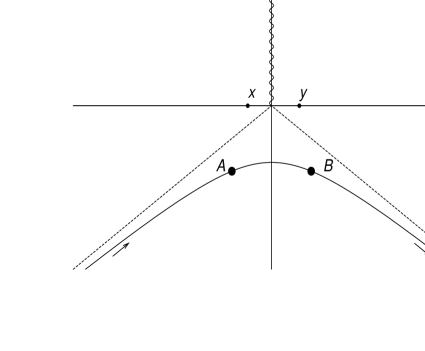
Figure 1: Schematic representation of the contour (solid line) in the complex-$x$ plane along which the WKB approximation to the Schrödinger equation (22) is derived. This contour passes through the two turning points $A$ and $B$ given in (23). These turning points are indicated by dots. For large $|x|$ the WKB contour approaches the centers of the asymptotic wedges (dashed lines) in which the eigenfunctions vanish exponentially as $|x|\to\infty$. The eigenfunctions are oscillatory on the WKB contour between $A$ and $B$. (This region is the complex generalization of the classically allowed region in conventional WKB theory.) Outside of this oscillatory region the eigenfunctions decay exponentially along the WKB contour. (These regions are the complex generalizations of the classically forbidden regions.) The eigenfunctions are analytic in the complex-$x$ plane except on the branch cut, which runs along the imaginary-$x$ axis from the origin to $i\infty$. To calculate the $\mathcal{C}$ operator the WKB approximation (20) to the eigenfunction $\phi_{n}$ is evaluated on the real-$x$ axis at the points $x$ and $y$, which are at a distance of order $1$ from the origin.

The WKB formulas (19) – (21) for the eigenfunctions $\phi_{n}(x)$ are valid in the complex-$x$ plane as well as on the real-$x$ axis. Our ultimate objective is to use these formulas to evaluate the sum (6) and thereby to determine the $\mathcal{C}$ operator. However, to demonstrate the techniques needed to evaluate this sum we will first show how to evaluate the sum in (5) that expresses the completeness condition and we will verify the (approximate) completeness of the WKB wave functions in (20).

We begin our analysis by finding the WKB approximation to the product $\phi_{n}(x)\phi_{n}(y)$. We will then perform the sum in (5) under the assumption that the arguments $x$ and $y$ of the eigenfunctions are real and of order 1. We must take $x$ and $y$ to be real because, as we will see, they will appear as arguments of a Dirac delta function, and the delta function is only defined for real argument. (The points $x$ and $y$ are shown in Fig. 1.) We will assume that $n\gg 1$, and therefore that $E_{n}\gg 1$. Under this assumption we can make the approximations

$$\left[E_{n}-x^{2}(ix)^{\delta}\right]^{-1/4}\sim E_{n}^{-1/4}\quad(\epsilon\to 0^{+})$$ (24)

and

$$\int_{A_{n}}^{x}dt\,\sqrt{E_{n}-t^{2}(it)^{\delta}}\sim I_{n}+\sqrt{E_{n}}x\quad(\epsilon\to 0^{+}),$$ (25)

where

$$I_{n}=\int_{A_{n}}^{0}dt\,\sqrt{E_{n}-t^{2}(it)^{\delta}}=\frac{\sqrt{\pi}}{2}E_{n}^{\frac{4+\delta}{4+2\delta}}\frac{\Gamma\left(\frac{3+\delta}{2+\delta}\right)}{\Gamma\left(\frac{8+3\delta}{4+2\delta}\right)}e^{\frac{i\pi\delta}{4+2\delta}}.$$ (26)

Using the trigonometric identity $2\sin\left(a+\frac{\pi}{4}\right)\sin\left(b+\frac{\pi}{4}\right)=\cos(a-b)+\sin(a+b)$, we obtain the WKB approximation to the product $\phi_{n}(x)\phi_{n}(y)$:

$$\phi_{n}(x)\phi_{n}(y) \sim \frac{(-1)^{n}}{\sqrt{E_{n}}\int_{A_{n}}^{B_{n}}dt\,\left[E_{n}-t^{2}(ix)^{\delta}\right]^{-1/2}}\left\{\cos\left[\frac{1}{\epsilon}\sqrt{E_{n}}(x-y)\right]\right.$$ (27)

$$\qquad\left.+\sin\left[\frac{2}{\epsilon}I_{n}+\frac{1}{\epsilon}\sqrt{E_{n}}(x+y)\right]\right\}\quad(\epsilon\to 0^{+}),$$

where the factor of $(-1)^{n}$ comes from the normalization condition (4).

We will see that this factor of $(-1)^{n}$ plays a crucial role in our evaluation of sums because oscillatory terms are suppressed relative to nonoscillatory terms. This factor arises because the phase-fixing condition (3) requires that the eigenfunctions $\phi_{n}(x)$ be $\mathcal{PT}$ symmetric. The harmonic oscillator ($\delta=0$) illustrates clearly the origin of the $(-1)^{n}$ factor. Requiring that the harmonic oscillator eigenfunctions be $\mathcal{PT}$ symmetric (that is, that they be functions of $ix$) means that they have the general form $\phi_{n}(x)=i^{n}e^{-x^{2}/2}He_{n}(x)$, where $He_{n}(x)$ is the usual Hermite polynomial. It is the extra factor of $i^{n}$ that gives rise to the factor of $(-1)^{n}$ in the normalization condition (4). The factor $(-1)^{n}$ persists for all $\delta>0$ BBJ .

Next, we use the quantization condition (19) to obtain the identity

$$\frac{2}{\epsilon}I_{n}=\left(n+\frac{1}{2}\right)\pi+\frac{1}{\epsilon}(I_{n}-I_{n}^{*}),$$ (28)

where $*$ denotes complex conjugation. This identity allows us to rewrite (27) as

$$\phi_{n}(x)\phi_{n}(y) \sim \frac{1}{\sqrt{E_{n}}\int_{A_{n}}^{B_{n}}dt\,\left[E_{n}-t^{2}(ix)^{\delta}\right]^{-1/2}}\left\{(-1)^{n}\cos\left[\frac{1}{\epsilon}\sqrt{E_{n}}(x-y)\right]\right.$$ (29)

$$\qquad\left.+\cos\left[\frac{1}{\epsilon}(I_{n}-I_{n}^{*})+\frac{1}{\epsilon}\sqrt{E_{n}}(x+y)\right]\right\}\quad(\epsilon\to 0^{+}),$$

The next step is to perform the sum over $n$. We do so by converting the sum to an integral using the general WKB density of states result

$$dE_{n}\,\frac{1}{2\epsilon}\int_{A_{n}}^{B_{n}}dx\,\left[E_{n}-V(x)\right]^{-1/2}=\pi\,dn\quad(\epsilon\to 0^{+}),$$ (30)

which is obtained by differentiating the quantization condition (19). Note that one must differentiate the endpoints as well as the integrand with respect to $E_{n}$, but the endpoints give a vanishing contribution because $E_{n}-V(A_{n})=E_{n}-V(B_{n})=0$, where the potential $V(x)=x^{2}(ix)^{\delta}$.

Let us substitute (30) into (5) and examine the sum over $n$ of the first term in the curly brackets in (29). Letting $r=\sqrt{E_{n}}/\epsilon$, the sum over $n$ in (5) becomes the integral

$$\frac{1}{\pi}\int_{0}^{\infty}dr\,\cos\left[r(x-y)\right]=\delta(x-y),$$ (31)

which is precisely the statement of completeness. Of course, this completeness result is only an approximation because the WKB approximation is only accurate for large $n$. Thus, the early terms in the sum over $n$ introduce an error in this result. This error is equivalent to changing the lower limit in the integral in (31) from $0$ to some other finite number $L$. However, the error that arises when $0$ is replaced by $L$ is finite, and when $x$ is near $y$, this error is small and may be neglected in comparison with $\delta(x-y)$, which is singular at $x=y$.

The second term in the curly brackets in (29) does not contribute to the sum over $n$ in (5) because there is a factor of $(-1)^{n}$ in this term. The rapid oscillation produced by this factor causes a cancellation between successive terms in the summation. As a result, this term contributes negligibly to the sum and the delta function result in (31) remains unchanged.

Next, we turn to the evaluation of the $\mathcal{C}$ operator in (6). Because there is no factor of $(-1)^{n}$ in this sum, it is now the first term in curly brackets in (29) that is unimportant and it is the second term that contributes. Converting this sum to an integral using (30), we obtain in coordinate space

$$\mathcal{C}(x,y)=\frac{1}{\pi}\int_{0}^{\infty}dr\,\cos\left[r(x+y)+iKr^{\frac{4+\delta}{2+\delta}}\epsilon^{\frac{2}{2+\delta}}\right],$$ (32)

where we have used the result that

$$I_{n}-I_{n}^{*}=iKE_{n}^{\frac{4+\delta}{4+2\delta}}$$ (33)

with the $n$-independent constant $K$ given by

$$K=\frac{\sqrt{\pi}\Gamma\left(\frac{3+\delta}{2+\delta}\right)}{\Gamma\left(\frac{8+3\delta}{4+2\delta}\right)}\sin\left(\frac{\pi\delta}{4+2\delta}\right).$$ (34)

For small $\epsilon$ the cosine function in (32) can be expanded into a two-term Taylor series and the first integral can be done as in (31):

$$\mathcal{C}(x,y)=\delta(x+y)-iK\epsilon^{\frac{2}{2+\delta}}\frac{1}{\pi}\int_{0}^{\infty}dr\,r^{\frac{4+\delta}{2+\delta}}\sin\left[r(x+y)\right].$$ (35)

To evaluate the remaining integral in (35), we transform to momentum space:

$$\mathcal{C}(p,q)=\int dx\,e^{-ipx}\int dy\,e^{iqy}\mathcal{C}(x,y).$$ (36)

The Fourier transform of the first term in (35) is $2\pi\delta(p+q)$, which is just the parity operator $\mathcal{P}(p,q)$ in momentum space. The Fourier transform of the second term in (35) is

$$-iK\epsilon^{\frac{2}{2+\delta}}\int dx\,e^{-ipx}\int dy\,e^{iqy}\int_{0}^{\infty}\frac{dr}{\pi}r^{\frac{4+\delta}{2+\delta}}\frac{1}{2i}\left[e^{ir(x+y)}-e^{-ir(x+y)}\right]$$

$$\quad=-\frac{K}{2\pi}\epsilon^{\frac{2}{2+\delta}}\int dx\int dy\int_{0}^{\infty}dr\,r^{\frac{4+\delta}{2+\delta}}\left[e^{i(r-p)x+i(q+r)y}-e^{-i(p+r)x+i(q-r)y}\right]$$

$$\quad=-2\pi K\epsilon^{\frac{2}{2+\delta}}\left[\theta(p)p^{\frac{4+\delta}{2+\delta}}-\theta(-p)(-p)^{\frac{4+\delta}{2+\delta}}\right]\delta(p+q),$$ (37)

where $\theta(t)=0\,(t<0)$, $\theta(t)=1\,(t\geq 0)$ is the step function. Thus, our result for the WKB approximation to the $\mathcal{C}$ operator in momentum space is

$$\mathcal{C}(p,q)=\mathcal{P}(p,q)-\epsilon^{\frac{2}{2+\delta}}\frac{\sqrt{\pi}\Gamma\left(\frac{3+\delta}{2+\delta}\right)}{\Gamma\left(\frac{8+3\delta}{4+2\delta}\right)}\sin\left(\frac{\pi\delta}{4+2\delta}\right)\left[\theta(p)p^{\frac{4+\delta}{2+\delta}}-\theta(-p)(-p)^{\frac{4+\delta}{2+\delta}}\right]\mathcal{P}(p,q).$$ (38)

Finally, we rewrite this result in the exponential form $\mathcal{C}=e^{Q}\mathcal{P}$ in (13), set $\epsilon=1$, and identify the function $Q$:

$$Q(p,q)=-\frac{\sqrt{\pi}\Gamma\left(\frac{3+\delta}{2+\delta}\right)}{\Gamma\left(\frac{8+3\delta}{4+2\delta}\right)}\sin\left(\frac{\pi\delta}{4+2\delta}\right)\left[\theta(p)p^{\frac{4+\delta}{2+\delta}}-\theta(-p)(-p)^{\frac{4+\delta}{2+\delta}}\right].$$ (39)

This is the principal result of our investigation.

III Discussion and Conclusions

We have found a physical-optics WKB approximation to the $\mathcal{C}$ operator in momentum space for the Hamiltonian in (1). Note that the results in (38) and (39) are valid for all $\delta\geq 0$. This represents a major advance over previous work; previously, the $\mathcal{C}$ operator was only determined for the special case of a cubic interaction term $\delta=1$. The methods used earlier were perturbative and were not as powerful as the nonperturbative semiclassical methods used in this paper.

The function $Q(p,q)$ exhibits the required symmetry properties mentioned earlier, namely, that it be an even function of $x$ and an odd function of $p$. Furthermore, because the sine function in (38) and (39) vanishes when $\delta=0$, we see that the $\mathcal{C}$ operator becomes identical with the parity operator $\mathcal{P}$ when the Hamiltonian is Hermitian in the conventional sense. The vanishing of $Q$ for the $\delta=0$ case can be traced back to the fact that for the harmonic oscillator the integral $I$ in (26) is real. Thus, $I-I^{*}=0$ in (28) and (29).

Note that the results in (38) and (39) simplify substantially when $\delta$ is an odd integer because the step function $\theta$ drops out of these formulas. For $\delta=2k+1$ we have

$$Q(p,q)=-\frac{\sqrt{\pi}\Gamma\left(\frac{4+2k}{3+2k}\right)}{\Gamma\left(\frac{11+6k}{6+4k}\right)}\sin\left(\frac{\pi(1+2k)}{6+4k}\right)p^{\frac{5+2k}{3+2k}}.$$ (40)

When $k=0$ (the case of a cubic theory) we have

$$Q(p,q)=-\frac{\sqrt{\pi}\Gamma(1/3)}{5\Gamma(5/6)}p^{5/3},$$

and when $k=\infty$ we have the especially simple result that

$$Q(p,q)=-2p.$$

Another special case is $\delta=2$. For this case the Hamiltonian (1) is quartic and

$$Q(p,q)=-\frac{\sqrt{2\pi}\Gamma(1/4)}{6\Gamma(3/4)}\left[\theta(p)p^{3/2}-\theta(-p)(-p)^{3/2}\right].$$

We hope to generalize the advance reported in this paper to noncubic $\mathcal{PT}$-symmetric quantum field theories, such as a $-g\varphi^{4}$ theory. A $-g\varphi^{4}$ quantum field theory in four-dimensional space-time is a remarkable model because it has a positive spectrum, is renormalizable, is asymptotically free BMS , and has a nonzero one-point Green’s function $G_{1}=\langle\varphi\rangle$. If we can perform the corresponding semiclassical approximation for a $-g\varphi^{4}$ quantum field theory, we may be able to elucidate the dynamics of the scalar sector in a variant of the standard electroweak model and possibly even predict the mass of the Higgs particle.

1. C. M. Bender and S. Boettcher, Phys. Rev. Lett. 80, 5243 (1998).
2. C. M. Bender and S. Boettcher and P. N. Meisinger, J. Math. Phys. 40, 2201 (1999).
3. E. Caliceti, S. Graffi, and M. Maioli, Comm. Math. Phys. 75, 51 (1980).
4. G. Lévai and M. Znojil, J. Phys. A33, 7165 (2000), and references therein.
5. B. Bagchi and C. Quesne, Phys. Lett. A300, 18 (2002).
6. Z. Ahmed, Phys. Lett. A294, 287 (2002); G. S. Japaridze, J. Phys. A35, 1709 (2002); A. Mostafazadeh, J. Math. Phys. 43, 205 (2002); ibid. 43, 2814 (2002); D. T. Trinh, PhD Thesis, University of Nice-Sophia Antipolis (2002), and references therein.
7. P. Dorey, C. Dunning and R. Tateo, J. Phys. A 34 L391 (2001); ibid. 34, 5679 (2001).
8. A. Mostafazadeh, J. Math. Phys. 43, 3944 (2002).
9. C. M. Bender, D. C. Brody, and H. F. Jones, Phys. Rev. Lett. 89, 270402 (2002).
10. C. M. Bender, D. C. Brody, and H. F. Jones, Am. J. Phys. 71, 1095 (2003).
11. C. M. Bender, P. N. Meisinger, and Q. Wang, J. Phys. A 36, 1973 (2003).
12. C. M. Bender, G. V. Dunne, P. N. Meisinger, and M. Ṣimṣek, Phys. Lett. A 281, 311-316 (2001).
13. C. M. Bender, J. Brod, A. T. Refig, and M. E. Reuter, J. Phys. A: Math. Gen. (to be published).
14. C. M. Bender, D. C. Brody, and H. F. Jones, hep-th/0402011.
15. C. M. Bender, D. C. Brody, and H. F. Jones, hep-th/0402183, to be published in Physical Review D.
16. C. M. Bender and S. A. Orszag, Advanced Mathematical Methods for Scientists and Engineers, (McGraw-Hill, New York, 1978), Chap. 10.
17. C. M. Bender, K. A. Milton, and V. M. Savage, Phys. Rev. D 62, 85001 (2000).