Worldsheet Geometry of Classical Solutions in String Field Theory

Abstract

We investigate classical solutions of string field theory proposed by Takahashi and Tanimoto in the case of even order polynomial functions. The modified BRS charge and the Feynman propagator of open string field theory expanded about the solution are specified by the Jenkins-Strebel quadratic differential, which describes the geometry of the string worldsheet. We show that the solution becomes nontrivial when two second order poles of the quadratic differential coincide on the unit disk.

1 Introduction

Classical solutions in string field theory (SFT) have been extensively investigated since Sen and Zwiebach[1] demonstrated that the Lorentz invariant classical solution of cubic open string field theory[2] corresponds to the nontrivial vacuum of the tachyonic potential. They evaluated the solution and the D25-brane tension using the level truncation scheme, [3] which truncates the string field at finite mass level. Surprisingly, their estimation of the tension with the level (4,8) approximation is within 1% of the expected value. Following their successful result, many works using the level truncation scheme have been carried out  and they support Sen’s conjecture [5].

However, the level truncation analysis is insufficient to prove and understand Sen’s conjecture completely. In particular, the worldsheet geometry behind the physics of tachyon condensation is lost when the string field is truncated at a finite level, because an infinite number of degrees of freedom are needed to describe string propagation on a worldsheet, which is a Riemann surface. One possible way to treat such problems is to consider an exact solution of equation of the motion of SFT, because it contains infinitely many degrees of freedom that are sufficient to describe a string worldsheet.

One attempt to construct a framework in which to treat the above-mentioned problem is represented by vacuum string field theory (VSFT).[7, 8, 9, 10, 11] The authors of Ref. rf:vsft proposed a pure ghost BRS charge as a kinetic operator of SFT after tachyon condensation, instead of finding an exact classical solution. This BRS charge ensures the disappearance of string excitations because it has a trivial cohomology. The kinetic operator in the Siegel gauge, obtained by anticommuting the BRS charge with $b_{0}$, is merely a c-number that has no geometrical meaning. Therefore the authors of Ref. rf:vsftghost proposed a regularization procedure using the kinetic operator $L_{0}$, which represents open string propagation on a flat worldsheet. They also made the observation that a closed string amplitude can be obtained by calculating a correlation function of the gauge invariant closed string operator[13] with the regularized propagator. Because the geometry of the worldsheet is same as in the case of ordinary open string theory, the effect of tachyon condensation is due to the regularization procedure. However, it is still not clear whether such a prescription is correct, as there is no principle to determine appropriate regularization procedure.

Another approach based on exact classical solutions is proposed in Ref. rf:TT. The classical solutions are called ‘universal solutions’, because they belong to the universal subspace of the open string Hilbert space[12]. In contrast to VSFT, the modified BRS charge obtained by expanding the SFT action around about the universal solution depends on the matter part of open string conformal field theory. Therefore the disappearance of open strings is a quite nontrivial problem in this approach. The solution is not unique but can be written in terms of a wide variety of functions on the complex plane. Each solution is uniquely specified by this function. In Ref. rf:TT the simplest solution with one real parameter is considered. It was found that at a boundary of the parameter space this solution is nontrivial, and at an interior of the parameter space it becomes a pure gauge solution. Subsequently, the cohomology of the modified BRS charge was investigated in Refs. [17] and [18]. There it was shown that at a boundary of parameter space the cohomology is trivial, and hence there is no open string.

After these works, Drukker made the important observation that the propagator obtained from a nontrivial universal solution generates a worldsheet whose boundary shrinks to a point[14, 15]. This mechanism can account to the disappearance of the open string from the worldsheet geometry. Actually, in Ref. rf:Drkr1 the worldsheet geometry of a purely closed string amplitude is studied.

In this paper, we elaborate on such geometrical treatment of string propagation by considering a class of universal solutions composed of polynomial functions. We identify the function specifying each solution as a quadratic differential on the complex plane. Quadratic differentials were used extensively in the development of the perturbation theory of SFT[19, 20, 21, 22, 23]. Feynman diagrams studied then are obtained by connecting a flat strip or cylinder whose geometry is locally trivial. A quadratic differential was used to understand the moduli space of Feynman diagrams with many propagators and vertices. Now our interest is in a single propagator deformed by a classical solution of string field theory. It has a locally nontrivial geometry represented by poles or zeros of the quadratic differential.

The paper is organized as follows. In §2 we review basic facts concerning universal solutions[16]. In particular, we focus on an algebraic property of the space of functions labeling each solution. In §3 we define the subspace of universal solutions composed of even-order polynomial functions explicitly, and we show that the solution is nontrivial when the zeros of the corresponding function are on the unit circle. In §4, we show that the function labeling each universal solution defines a quadratic differential describing the world sheet geometry, and plot some examples of trajectory diagrams.

2 Universal solutions

A universal solution[16] is a background independent, Lorentz invariant classical solution of cubic open string field theory[2]. Such a solution is given by

$$\Psi_{0}=Q_{L}(F){\cal I}-C_{L}\left(\frac{(\partial F)^{2}}{1+F^{2}}\right){\cal I},$$ (1)

where ${\cal I}$ is the identity string field. $F$ is a function defined on the complex plane. It satisfies the conditions

$$F(-1/w)=F(w),\quad F(\pm i)=0.$$ (2)

The quantities $Q_{L}(F)$ and $C_{L}(G)$ are defined by

$$Q_{L}(F)=\int_{\gamma_{L}}dw\,F(w)J_{B}(w),\quad C_{L}(G)=\int_{\gamma_{L}}dw\,G(w)c(w),$$ (3)

where the path $\gamma_{L}$ traverses in the counterclockwise direction on the left half of the unit circle. $J_{B}(w)$ and $c(w)$ are the BRS current and conformal ghost, respectively. We analyze the modified BRS charge  obtained by shifting the string field around the solutions instead of analyzing Eq. (1) directly, as this is technically simpler. Rewriting $F(w)$ as $g(w)-1$, we can compute the BRS charge as[16]

$$Q_{g}\Psi = Q_{B}\Psi+\Psi_{0}*\Psi+\Psi*\Psi_{0}$$ (4)

$$= \left[Q\left(g\right)-C\left(\frac{(\partial g)^{2}}{g}\right)\right]\Psi,$$

where $Q(f)$ and $C(f)$ are defined by integrals over the unit circle $\gamma$ as

$$Q(f)=\oint_{\gamma}dw\,f(w)J_{B}(w),\quad C(f)=\oint_{\gamma}dw\,f(w)\,c(w).$$ (5)

From the condition (2), $g(w)$ must satisfy

$$g\left(-\frac{1}{w}\right) = g(w),$$ (6)

$$g\left(\pm i\right) = 1.$$ (7)

We refer to a function $g(w)$ satisfying Eqs. (6) and (7) as a universal function, because it specifies the universal solution and the BRS charge uniquely. It is used frequently in the following. Equation (4) allows us to obtain various BRS charges by choosing the universal function. Note that the universal functions form an Abelian group with respect to ordinary multiplication of functions. More precisely, let $\mathcal{F}$ be the set of all universal functions. Then it is easy to see that

$$f,g\in\mathcal{F}\rightarrow fg\in\mathcal{F},$$ (8)

using Eqs. (6) and (7). Furthermore, the identity element and the inverse are given by $g(w)=1$ and $1/g(w)$, respectively. Thus $\mathcal{F}$ is an Abelian group with respect to ordinary multiplication.

As shown in Refs. [16] and [17], there exists a homomorphism from $\mathcal{F}$ to the space of field redefinitions acting on the string field. To see this, let us define the conserved ghost current $q(h)$ as

$$q(h)=\oint_{\gamma}dw\,h(w)\left(J_{gh}(w)-\frac{1}{w}\right),$$ (9)

where $J_{gh}(w)=:c(w)b(w):$ is the ghost number current. Using this current, we can construct a field redefinition operator as

$$E_{g}=e^{q(\log g)}.$$ (10)

Applying this operator to the BRS charge (4), we have the identity given in Ref. rf:KT,

$$E_{f}Q_{g}E_{f}^{-1}=Q_{fg}.$$ (11)

From the above equation, we easily show that

$$E_{f}E_{g}=E_{fg}.$$ (12)

Thus, the homomorphism mentioned above is given by $g\rightarrow E_{g}$. Moreover, this Abelian group is also homomorphic to the Abelian subgroup of the gauge group of SFT. Now, recall that the universal solution (1) can be rewritten as the pure gauge expression

$$\Psi_{0}=U_{g}*Q_{B}{U_{g}}^{-1},$$ (13)

where $U_{g}=e^{q_{L}(\log g){\cal I}}$ is an element of the gauge group of SFT, and $q_{L}(\log g)$ is an integral of $\log g(w)J_{gh}(w)$ on the left half of the unit circle.[16] Using formulas given in Ref. rf:TT, we can see that

$$U_{f}*U_{g}=U_{fg}$$ (14)

holds. The above equation gives a homomorphism from the space of universal functions $\mathcal{F}$ to the subspace of the SFT gauge group generated by $U_{g}$. Therefore, we can determine the structure of this subgroup by analyzing $\mathcal{F}$.

In order to classify elements of $\mathcal{F}$, it is convenient to focus on the operator $E_{g}$. It acts on the string field as a field redefinition given by $\Psi^{\prime}=E_{g}\Psi$. Using the fact that $E_{g}$ leaves string field vertices invariant[16], we can show the formal identity

$$S[Q_{B},\Psi]=S[Q_{g},\Psi^{\prime}],$$ (15)

where

$$S[Q_{g},\Psi]=\int\frac{1}{2}\Psi*Q_{g}\Psi+\int\frac{1}{3}\Psi*\Psi*\Psi$$ (16)

is the cubic open SFT action[2] with BRS operator $Q_{g}$. If $E_{g}$ is a regular transformation on the string field, Eq. (15) implies that SFT with the BRS operator $Q_{g}$ is equivalent to the original theory, and the classical solution labeled by $g(w)$ is merely a pure gauge solution. However, it happens that $E_{g}$ becomes singular and the transformation on the string field is ill-defined, because it is an infinite-dimensional linear transformation on the component fields of $\Psi$. For example, such a singularity can be seen from the normal ordering constant of $E_{g}$:

$$E_{g}=N:E_{g}:.$$ (17)

If $N$ diverges, the transformation $E_{g}$ is singular and ill-defined, and the corresponding classical solution is expected to be nontrivial. Therefore, we define the singular transformation $E_{g}$ as a transformation whose normal ordering constant is divergent, and the nontrivial element of $\mathcal{F}$ as the universal function $g(w)$ associated with a singular transformation.

Our goal is to obtain all singular solutions up to regular field redefinitions and to classify them. This is accomplished as follows. First, let $\mathcal{F}_{r}$ be a subgroup of $\mathcal{F}$ giving a regular transformation. Then, the space of inequivalent solutions is the coset

$$\mathcal{K}=\mathcal{F}/\mathcal{F}_{r}.$$ (18)

In particular, the identity element of $\mathcal{K}$ corresponds to the ordinary BRS charges $Q_{B}$. Other elements represent BRS charges that are equivalent neither to $Q_{B}$ nor to each other.

It is surprising that a classification of exact solutions of SFT — which involves the complicated structure of the star product in general — reduces to the significantly simpler problem of determining the Abelian group of the multiplication of universal functions.

3 Even finite universal solutions

Let us consider a universal function containing finite powers of $w$. It can be decomposed as

$$g(w)=g_{+}(w)+g_{-}(w),$$ (19)

where $g_{+}(w)$ and $g_{-}(w)$ are even and odd functions of $w$, respectively. Imposing Eq. (7) on Eq. (19), we see that these functions must satisfy the relation

$$g_{+}(\pm i)=1,\quad g_{-}(\pm i)=0.$$ (20)

We can consider the subset of universal functions satisfying $g_{-}(w)=0$, as in this case $g(w)$ still satisfies the condition (7) and actually belongs to the subgroup of $\mathcal{F}$ generated by even polynomial functions. In the following, we limit ourself to this case, because $g(w)$ has a simpler structure than that in the case involving the odd part. In this case, the Laurent expansion of $g(w)$ is given by

$$g(w)=\sum_{n=0}^{N}a_{n}\left(w^{2n}+w^{-2n}\right),$$ (21)

where $N$ is a positive integer and we have used Eq. (6). It is convenient to rewrite Eq. (21) into the rational form

$$g(w)=\frac{P_{2N}(w^{2})}{w^{2N}},$$ (22)

where $P_{2N}$ is a $2N$th order polynomial of $w^{2}$. From Eq. (6), it is clear that if $X$ is a zero of $P_{2N}$, then $X^{-1}$ also must be a zero of $P_{2N}$. Thus, the universal function can be expressed as

$$g(w)=\lambda\prod_{k=1}^{N}\frac{\left(w^{2}-X_{k}\right)\left(w^{2}-{X_{k}}^{-1}\right)}{w^{2}},$$ (23)

where $X_{k}\ (k=1,\cdots,N)$ are complex parameters. Because $X_{k}$ and ${X_{k}}^{-1}$ appear in pairs, we can set $|X_{k}|\leq 1$ without loss of generality. The constant $\lambda$ in Eq. (23) is determined from Eq. (7) as

$$\lambda=\prod_{k=1}^{N}\frac{-1}{\left(1+X_{k}\right)\left(1+{X_{k}}^{-1}\right)}.$$ (24)

Note that Eq. (23) can be represented as a product of ‘$N=1$’ universal functions as

$$g(w)=\prod_{k=1}^{N}g_{X_{k}}(w),$$ (25)

where

$$g_{X_{k}}(w) = \lambda_{k}\frac{\left(w^{2}-X_{k}\right)\left(w^{2}-{X_{k}}^{-1}\right)}{w^{2}},$$ (26)

$$\lambda_{k} = \frac{-1}{\left(1+X_{k}\right)\left(1+{X_{k}}^{-1}\right)}.$$ (27)

A further condition must be imposed on the set of parameters $\{X_{k}\}$ that results from the Hermicity of the BRS charge. As shown in Appendix A, the Hermicity of $Q_{g}$ is equivalent to $g(w)$ being purely real on the unit disk. From Eqs. (25) – (27), we find that

$$\overline{g(w)}=\prod_{k=1}^{N}g_{\overline{X_{k}}}(w)$$ (28)

is satisfied on the unit disk. Then, from Eqs. (25) and (28), the Hermicity condition reads

$$\overline{X_{k}}=X_{\sigma(k)}\quad(k=1,2,\cdots,N).$$ (29)

Here, $\sigma$ is a permutation that sends $\{1,2,\cdots,N\}$ to $\{\sigma(1),\sigma(2),\cdots,\sigma(N)\}$. Thus we have obtained the class of universal solutions defined by Eqs. (23), (24) and (29). We call the solutions in this class ‘even finite universal solutions’. Each solution is labeled by a set of parameters $\{X_{k}\}$ which satisfies Eq. (29).

Now that the even finite solutions are defined explicitly, we can specify nontrivial solutions among them by carrying out the normal ordering defined by Eq. (10) on the field redefinition operator $E_{g}$. If we write $h(w)=\log g(w)$, this operation is expressed as

$$e^{q(h)}=e^{\frac{1}{2}[{q^{+}(h)},{q^{-}(h)}]}:e^{q(h)}:,$$ (30)

where ${q^{+}(h)}$ and ${q^{-}(h)}$ are the positive and negative frequency parts of $q(h)$, respectively. Using formulas given in Appendix B, we obtain

$$E_{g}=\left[\prod_{k=1}^{N}\frac{1}{1-X_{k}^{2}}\right]\left[\prod_{k<l}^{N}\frac{1}{(1-X_{k}X_{l})^{2}}\right]:E_{g}:.$$ (31)

Because $|X_{k}|\leq 1$, the factor $1-X_{k}X_{l}$ in Eq. (31) becomes zero if and only if both $X_{k}$ and $X_{l}$ are on the unit circle. Furthermore, the quantity $1-{X_{k}}^{2}$ in Eq. (31) becomes zero when $X_{k}=\pm 1$, where $X_{k}$ is also on the unit circle. Therefore, $E_{g}$ becomes a singular field redefinition if at least one of the elements of $\{X_{k}\}$ lies on the unit circle. Because a regular $E_{g}$ corresponds to trivial pure gauge transformation[16], we conclude that an even finite universal solution is nontrivial if and only if some zeros of $g(w)$ lie on the unit circle.

Our next task is to obtain an ‘irreducible’ nontrivial solution by removing the regular part from singular solution. For example, consider a nontrivial even finite solution given by a universal function $g(w)$ that has some zeros on the unit circle. Suppose that there exists the factorization

$$g(w)=g_{r}(w)\tilde{g}(w),$$ (32)

where $g_{r}(w)$ and $\tilde{g}(w)$ are even finite universal functions such that $g_{r}(w)$ has all zeros inside the unit disk whereas $\tilde{g}(w)$ has some zeros on the unit circle. Then, using Eq. (11), we can remove $g_{r}(w)$ through a regular field redefinition and thereby obtain the reduced universal function $\tilde{g}(w)$.

Though we have assumed the factorization (32) , at this stage, we do not know whether it is always possible. In the following, we prove that in fact it is the case. To prove the factorization, we must take into account the Hermicity condition (29). First, it is useful to consider a special element of $\mathcal{F}$ such that the permutation of Eq. (29) is cyclic. In this case, we can set

$$\overline{X_{k}} = X_{k+1},\quad(k=1,\cdots,N-1),$$ (33)

$$\overline{X_{N}} = X_{1},$$ (34)

without loss of generality. From Eqs. (33) and (34), it is clear that the set $\{X_{k}\}\ (k=1,\cdots,N)$ can be expressed as

$$\{\underbrace{X_{1},\overline{X_{1}},X_{1},\overline{X_{1}},\cdots}_{N}\},$$ (35)

and the universal function has the expression

$$g^{c}_{X_{1}}(w)=\left\{g_{X_{1}}(w)\right\}^{n}\left\{g_{\overline{X_{1}}}(w)\right\}^{N-n},$$ (36)

where the superscript $c$ denotes “cyclic” and $n$ is given by

$$n=\begin{cases}\frac{N}{2}&N\in 2\mathbb{N},\\ \frac{N-1}{2}&N\in 2\mathbb{N}-1.\\ \end{cases}$$ (37)

From Eq. (35), we find that $g^{c}_{X_{1}}$ must be either irreducible or entirely regular, because it depends on only the single parameter $X_{1}$.

Let us now return to the case of general even finite universal functions with the permutation $\sigma$. It is well known that any permutation can be written as a direct sum of cyclic permutations. This implies that $g(w)$ factorizes into a product of ‘cyclic’ functions defined by Eq. (36) as

$$g(w)=g^{c}_{X_{1}}(w)g^{c}_{X_{2}}(w)\dotsb g^{c}_{X_{M}}(w),$$ (38)

where $M$ is the number of cyclic permutations contained in $\sigma$. If $X_{k}$ is inside the unit disk, we can remove $g^{c}_{X_{k}}(w)$ by applying the field redefinition operation on the BRS operator. Let us assume that the elements of $\{X_{1},X_{2},\cdots,X_{m}\}\ (m<M)$ are located on the unit circle and other zeros are inside unit disk. Then, $g(w)$ factorizes into singular and nonsingular parts as in Eq. (32). Removing the regular part from $g(w)$, we obtain the irreducible universal function

$$\tilde{g}(w)=g^{c}_{X_{1}}(w)\dotsb g^{c}_{X_{m}}(w),.$$ (39)

Therefore, we conclude that if we apply a field redefinition to the BRS operator, any nontrivial even finite universal solution can be reduced to a solution such that all zeros of $g(w)$ lie on the unit circle. In other words, we have proved that the coset space $\mathcal{K}$ defined by Eq. (18) is the set of all universal functions whose zeros are all on the unit circle.

We have seen that the unit circle and the zeros of the universal function play an important role in the classification of the even finite universal solutions. We consider the geometrical nature of these objects in the next section.

4 Feynman propagator in Siegel gauge

4.1 Quadratic differentials

In the following discussion, we take $g(w)$ to be an even universal function defined by Eqs. (23), (24) and (29). The kinetic operator of SFT in the Siegel gauge is obtained by taking the anticommutator of the BRS charge with $b_{0}$. The result is[18]

$$L_{v} = \{Q_{g},b_{0}\}$$

$$= \sum_{n}v_{n}L^{\prime}_{-n}+a,$$

where $v_{n}$ is defined by

$$wg(w)=\sum_{n}v_{n}w^{-n+1},$$ (40)

$L^{\prime}_{n}=L_{n}+nq_{n}+\delta_{n,0}$ is the twisted Virasoro generator with central charge $c=24$,and $a$ is a constant that comes from the pure ghost term of $Q_{g}$. Thus the kinetic operator is specified by the vector field

$$v(w)=wg(w).$$ (41)

This vector field satisfies the conditions,

$$v(w) = -w^{2}v\left(-\frac{1}{w}\right),$$ (42)

$$v(\pm i) = \pm i,$$ (43)

where we have used Eqs. (6) and (7). The Feynman propagator is the inverse of the kinetic operator. Introducing Schwinger parameter, we have

$$\frac{1}{L_{v}}=\int_{0}^{\infty}dt\,e^{-tL_{v}}.$$ (44)

We can show the Hermicity of $L_{v}$ using an argument similar to that given in the Appendix A. Thus, this propagator represents unitary time evolution on the worldsheet. The integrand of Eq. (44) acts on a primary field of dimension $d$ in the twisted CFT as

$$e^{tL_{v}}\phi(w)e^{-tL_{v}}=\left(\frac{dz_{t}(w)}{dw}\right)^{d}\phi(z_{t}(w)),$$ (45)

where $z_{t}(w)$ is a one-parameter family of conformal maps. It is well known that $z_{t}(w)$ is given by the formula[24, 25]

$$z_{t}(w)=e^{tv(w)\partial_{w}}w.$$ (46)

In principle, we can obtain an expression of $z_{t}(w)$ as a formal power series in $t$. In order to obtain a closed expression for this conformal map, it is useful to consider the differential equation that follows from Eq. (46) [24, 25],

$$v(w)\partial_{w}z_{t}(w)=v(z_{t}(w)).$$ (47)

When $v(w)$ is given, one can integrate the above equation and obtain a finite conformal map.

In order to investigate the worldsheet geometry, it is useful to rewrite Eq. (47) as an equation for a meromorphic one form and to square this. Doing so, we obtain

$$\frac{dw^{2}}{v(w)^{2}}=\frac{dz_{t}^{2}}{v(z_{t})^{2}}.$$ (48)

Here, ${dz}^{2}=dzdz$ is a tensor product of one forms. The above equation suggests the existence of a meromorphic quadratic differential[26] associated with the open string propagator,

$$\varphi(z)\,dz^{2},\quad\varphi(z)=\frac{1}{{v(z)}^{2}},$$ (49)

where $z$ is the coordinate of the complex plane.

Once the quadratic differential is introduced, we can interpret Eq. (48) as follows. Let us consider a region $\mathcal{R}$ in the complex plane such that $z_{t}(w)$ is single valued. Then Eq. (48) defines a one-parameter family of line elements for which values of the quadratic differential are equal. Recall that a trajectory of a quadratic differential is defined as an integral curve of line elements on $\mathcal{R}$ which leaves $\arg\varphi(z)dz^{2}$ invariant.[26] Therefore, the integral curve defined by Eq. (48) is a trajectory of the quadratic differential (49). In Appendix C we show that $z_{t}(w)$ actually defines horizontal trajectories.

Among various trajectories of the quadratic differential, the unit circle plays a special role. In fact, it turns out that it is always a vertical trajectory. This can be seen by introducing the parameterization $w=e^{i\theta}$. Then, the value of the quadratic differential on the unit circle is evaluated as

$$\frac{dw^{2}}{v(w)^{2}}=-\frac{d\theta^{2}}{g(e^{i\theta})^{2}}\leq 0,$$ (50)

where we have used Eq. (41) and the fact that $g(w)$ is purely real on the unit circle. In addition, using Eqs. (42) and (43), we can see that the quadratic differential is invariant with respect to the BPZ inversion $z^{\prime}=-1/z$:

$$\frac{dz^{2}}{v(z)^{2}}=\frac{{dz^{\prime}}^{2}}{v(z^{\prime})^{2}}.$$ (51)

Figure 1: A horizontal trajectory starting from unit circle.

From the above result, it is sufficient to consider the region inside unit disk, because trajectories outside the unit disk are the BPZ inversions of trajectories inside the region. Taking the starting point $w$ to be on the unit circle, one can uniquely determine a horizontal trajectory that goes inside unit circle, as illustrated in Fig. 1. Thus we can interpret $z_{t}(w)$ as the time evolution along the horizontal trajectory starting from the unit circle, with coordinate $w$.

The geometry of a worldsheet is determined by the trajectory structure of its quadratic differential. In particular, vertical trajectories correspond to equal time lines of conformal fields. Because a quadratic differential is a coordinate independent object, its trajectory structure is determined by the types of poles or zeros and the coefficients of the quadratic differential near second order poles, which are also coordinate independent.[26]

4.2 Regular solutions

From Eqs. (23) and (41), the general form of the quadratic differential obtained from an even finite universal solution is given by

$$\varphi(z)dz^{2}=\frac{1}{\lambda^{2}}\frac{z^{4N-2}}{\prod_{k=1}^{N}(z^{2}-X_{k})^{2}(z^{2}-{X_{k}}^{-1})^{2}}\,dz^{2}.$$ (52)

Now we investigate the trajectory structure of regular solutions for which all of the $X_{k}$ are inside the unit disk. There are $2N$ second order poles inside the unit disk, $2N$ second order poles outside the unit disk, and a zero of order $(4N-2)$ at the origin. Here we list some features of the trajectory diagrams obtained from Eq. (52).

• The trajectory structure near a second order pole is determined by the asymptotic form of the quadratic differential near the pole. Near a second order pole $\sqrt{X}$, this asymptotic form is given by

  $$\phi(z)dz^{2}\sim\frac{a_{-2}}{(z-\sqrt{X})^{2}}dz^{2},$$ (53)

  where $a_{-2}$ is a constant. If $a_{-2}$ is real and positive, the vertical trajectory is a closed curve surrounding the pole (see Fig. 2). For convenience, we consider the cases in which all poles have positive coefficient.

• For a second order pole $\sqrt{X_{k}}$ inside the unit disk, there always exists the other pole $\sqrt{X_{\sigma(k)}^{-1}}$ outside the unit disk (Fig. 3). This follows from the Hermicity condition (29). Such pairs of poles play an important role in determining the worldsheet geometry.

Figure 2: Vertical trajectory around a second order pole.

Figure 3: A pole $X_{k}$ is always paired with its inverse $X_{k}^{-1}$. From the Hermicity condition, there always exists $X_{\sigma(k)}^{-1}$, which is complex conjugate of $X_{k}^{-1}$.

In order to draw vertical trajectories in the $z$ plane, it is convenient to introduce the flat (or ‘distinguished’) coordinate of the quadratic differential (52):

$$d\rho^{2}=\varphi(z)dz^{2}.$$ (54)

Integrating the above equation, we find

$$\rho=\int^{z}\sqrt{\phi(z^{\prime})}\,dz^{\prime}=\Phi(z).$$ (55)

where $\rho$ is defined up to its sign and an additive constant. Because a vertical trajectory in this flat coordinate is a vertical straight line (i.e. a curve that satisfy $\mathrm{Re}\,\rho=$ const. ) a vertical trajectory in the $z$ plane is given by the condition

$$\mathrm{Re}(\Phi(z))=r.\quad(r\in\mathbb{R})$$ (56)

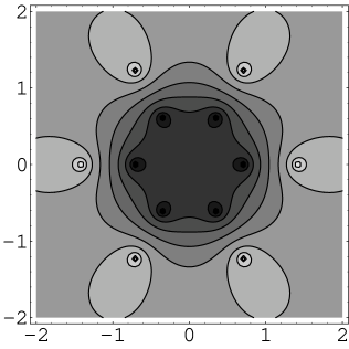
Figure 4: Vertical trajectories of $N=3$ function with $X_{1}=e^{2\pi i/3}/2,X_{2}=1/2$. In this case, $X_{2}$ forced to be real.

Here we give some examples. Using the general expression of the universal function (52), we plot vertical trajectories of $N=1$ (Fig. 6), $N=2$ (Fig. 6) and $N=3$ (Fig. 4) functions. The positions of the poles are chosen so as to satisfy Eq. (29).

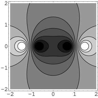
Figure 5: Vertical trajectories of the $N=1$ function with $X_{1}=1/2$. From the Hermicity condition, the poles must be real or purely imaginary. The shade of a region represents the worldsheet ‘time’ $\tau=\mathrm{Re}(\rho)$, with increasing brightness corresponding to increasing time.

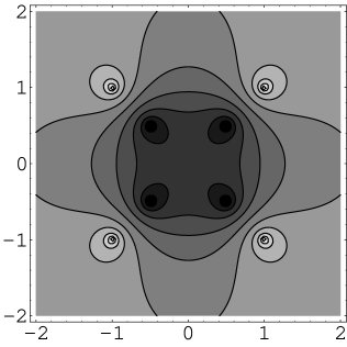
Figure 6: Vertical trajectories of the $N=2$ function with $X_{1}=i/2$. The four poles inside the unit disk correspond to the two square roots of $X_{1}$ and the two square roots of $\overline{X_{1}}$.

4.3 Example of an open string worldsheet with $N=3$

As seen in the figures 4 and 6, an $N\geq 2$ diagram has many second order poles in general. It looks like a worldsheet of interacting strings, because a second order pole corresponds to an incoming or outgoing source of an open string state in the ordinary open string CFT. However, these graphs must describe the propagation of a single string, as we consider only single propagator. As we see below, it turns out that most poles are dummies, and only two pairs of poles couple with string states.

In order to specify the region corresponding to an open string in the trajectory diagram, we start from an alternative derivation of the quadratic differential based on a gauge invariant treatment. Suppose that a BRS charge with a universal function $g(w)$ is obtained from ordinary BRS charge $Q_{B}$ by twisted conformal transformation

$$\mathcal{N}Q_{g}=U^{\prime}_{f}Q_{B}{U^{\prime}_{f}}^{-1},$$ (57)

where $U^{\prime}_{f}$ is a finite conformal transformation with the map $z=f(w)$ in the twisted CFT, and $\mathcal{N}$ is a real constant. Then, using the fact that the BRS current transforms like a weight two operator , up to the pure ghost term[18], and using the relation $J^{\prime}_{B}(w)=wJ_{B}(w)$, where $J^{\prime}_{B}(w)$ is the twisted BRS current, we can compute the $J_{B}$ part of the right-hand side of Eq. (57) as

$$\oint_{\gamma}dw\,U^{\prime}_{f}J_{B}(w){U^{\prime}_{f}}^{-1} = \oint_{\gamma}dw\,\frac{w}{z}\left(\frac{dz}{dw}\right)^{2}J^{\prime}_{B}(z)$$ (58)

$$= \oint_{\gamma}dz\,\frac{w}{z}\left(\frac{dz}{dw}\right)J^{\prime}_{B}(z).$$

In the second line of the above equation, we assume that $z$ winds once on the unit circle. Comparing this expression to the left-hand side of Eq. (57), we obtain

$$\mathcal{N}g(z)=\frac{w}{z}\frac{dz}{dw},$$ (59)

or, rewriting the above equation as a one form and squaring, we obtain

$$\frac{dz^{2}}{v(z)^{2}}=\mathcal{N}^{2}\frac{dw^{2}}{w^{2}}.$$ (60)

The right-hand side of Eq. (60) is the quadratic differential in the disk coordinate $w$. Indeed, we can obtain Eq. (54) from Eq. (60) by using the coordinate transformation $w=e^{\mathcal{N}\rho}$. Therefore, the conformal transformation $z=f(w)$ maps a disk worldsheet into a certain region in the $z$ plane, and Eq. (60) represents a coordinate transformation of the quadratic differential.

As an example, we derive the conformal map associated with the one parameter family of $N=3$ solutions (which includes the case of Fig.  4) , i.e.

$$X_{1}=r^{2}e^{\frac{2}{3}i\pi},\ X_{2}=r^{2},\ X_{3}=r^{2}e^{-\frac{2}{3}i\pi}\quad(0\leq r<1).$$ (61)

From Eq. (52), the quadratic differential is given by

$$\phi(z)dz^{2}=\frac{(1+r^{6})^{4}}{r^{12}}\frac{z^{10}dz^{2}}{(z^{6}-r^{6})^{2}(z^{6}-r^{-6})^{2}},$$ (62)

and the differential equation (59) becomes

$$-\frac{(1+r^{6})^{2}}{r^{6}}\frac{z^{5}dz}{(z^{6}-r^{6})(z^{6}-r^{-6})}=\mathcal{N}\frac{dw}{w}.$$ (63)

We can obtain an explicit expression of $z=f(w)$ by integrating Eq. (63). Note that there are two unknown constants, $\mathcal{N}$ and an integration constant. They are determined from the condition that the entire unit circle be fixed with respect to the conformal map. This condition ensures the gluing rule of states in the SFT with BRS charge $Q_{g}$, because SFT vertices are defined by the overlap conditions on the unit circle. In this example, these constants are fixed as follows:

• $\mathcal{N}$ is fixed so that the closed path around the unit circle winds once in both $w$ and $z$ planes. This condition is already assumed in Eq. (58). Then, from Eq. (63) we obtain $\mathcal{N}=(1+r^{6})/(1-r^{6})$.

• The integration constant in Eq. (63) is fixed by the condition $w=\pm i\Rightarrow z=\pm i$, which fixes the open string midpoint. This condition yields the operator $U^{\prime}_{f}$ generated by the midpoint preserving operator $K^{\prime}_{2m}=L^{\prime}_{2m}-L^{\prime}_{-2m}$ [2].

Fixing these constant, we find the local expression for the conformal map

$$z=f(w)=\left(\frac{w^{6}+r^{6}}{r^{6}w^{6}+1}\right)^{\frac{1}{6}}.$$ (64)

Because we already know that the equal time lines in the $z$ plane are always on the vertical trajectory depicted in Fig. 4, all we need is to identify the boundaries and the image of the upper half $w$ plane. This can be accomplished easily by using (64). Figure 7 shows how the upper half of $w$ plane is mapped into the $z$ plane. In both $z$ and $w$ coordinates, open string worldsheets constitute upper half planes, while open string boundaries in the $z$ plane consist of two line segments connecting second order poles on the real axis. The small semicircle around $w=0$ goes around two second order poles on the real axis and two spurious second order poles in the upper half $z$ plane. Contrastingly, a semicircle near $|w|=1$ is mapped to a single curve near $|z|=1$, because it does not meet brunch cuts in the $w$ plane.

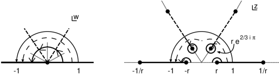
Figure 7: Conformal map of the $N=3$ solution. Four poles inside upper half $z$ planes are ‘dummies’.

Similar results are obtained for different $N$ cases: most second order poles are dummies, and an open string boundary is a vertical trajectory that connects two second order poles on the real axis.

Though we have given an example of the identification of an open string worldsheet explicitly, such analysis is not necessary in determining the singularity of a solution, as it depends only on the local structure of the quadratic differential.

4.4 Singular solutions

In the case of singular solutions, any universal function can be taken to have all of its zeros on the unit circle. In the language of quadratic differentials, these zeros correspond to second order poles on the unit circle, as seen from Eq. (52). Because a pole $\sqrt{X_{k}}$ inside the unit disk is always paired with another pole $\sqrt{\overline{X_{k}^{-1}}}$ outside the unit disk, they coincide on the unit circle and become a single fourth order pole. Thus we conclude that the quadratic differential associated with a singular even finite universal solution must have poles of fourth or more higher order on the unit circle. Figure 8 illustrates the local trajectory structure near the unit circle. Figures 10 and 10 are trajectory diagrams of the $N=2$ solutions.

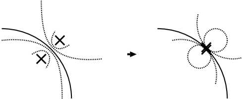
Figure 8: A fourth order pole on the unit disk can be regarded as coincident second order poles.

Figure 9: Vertical trajectories of the $N=2$ solution with $X_{1}=e^{i\pi/2}/2$. Two second order poles are situated across from each other with respect to the unit circle.

Figure 10: Vertical trajectories of the $N=2$ solution with $X_{1}=e^{i\pi/2}$. A pair of second order poles becomes a single fourth order pole.

The result obtained above implies that all singular even finite solutions correspond to the no open string vacuum, because the local structure of the quadratic differential around a pole of fourth or more higher order is quite different from that of a pole of second order, which can be mapped to a flat strip. This implies that the Feynman propagator around a singular solution never couples with open string states. To make this observation more evident, we must analyze the spectrum or the cohomology of the BRS charge for singular solutions.

5 Conclusions

In this paper we have investigated a class of universal solutions specified by even polynomial universal functions and showed that a solution becomes nontrivial when the zeros of the universal function are on the unit circle. Furthermore, we have found that the universal function associated with each solution gives a meromorphic quadratic differential on the complex plane, and that the solution becomes nontrivial when second order poles coincide on the unit circle. Such a relation between nontrivial universal solution and poles on the unit circle has been pointed out by Drukker[14, 15]. Our result confirms his conjecture in the case of even order polynomial universal functions. Now it becomes clear that the universal solution uniquely determines the string propagation around itself, and the geometrical nature of the worldsheet swept by the string are entirely encoded in the universal function. Furthermore, we know that a universal solution can be formally expressed as a pure gauge solution whose gauge group element is uniquely specified by the universal function. Therefore, these facts imply that the gauge group of SFT contains rich degrees of freedom that correspond to various string worldsheets.

We conjecture that all nontrivial solutions considered in this paper yield tachyon condensation and the disappearance of open strings, because the propagators never couple to open string states. Though we have obtained a wide variety of nontrivial solutions, according to Sen’s conjecture, the stable vacuum of the tachyonic potential must be unique. If Sen’s conjecture holds, these solutions must be related to each other by some transformations. Therefore it is important to investigate whether the nontrivial solutions are equivalent. Furthermore, to confirm the conjecture that nontrivial universal solutions yield closed string propagation, we must calculate closed string amplitudes using these solutions. It has been suggest that a zero momentum dilaton lives on the shrunken boundary[11, 14]. It would be interesting to calculate this amplitude explicitly in same manner as Ref. rf:TZ2.

Although we have investigated even finite universal solutions only, it would be interesting to consider other cases. First, we must consider nonpolynomial universal functions, because they appear as the inverse elements of polynomial universal functions with respect to the Abelian multiplication discussed in §2. Another example of a nonpolynomial type solution that yields a pure ghost BRS charge is given in Ref. rf:Drkr2. In addition, polynomial-type solutions with odd parts also must be considered.

Appendix A Hermicity of the BRS Charge

Let $g(w)$ be a universal function in $\mathcal{F}$ with a finite Laurent expansion. It can be expanded as

$$g(w)=\sum_{n=-M}^{M}g_{n}w^{-n},$$ (65)

where $M$ is a positive integer. First, we investigate the Hermicity condition of $Q(g)$. A mode expansion of $J_{B}(w)$ is given by

$$J_{B}(w)=\sum_{n}Q_{n}w^{-n-1}.$$ (66)

Then, using Eqs. (65), (66) and (5), the mode expansion of $Q(g)$ is found to be

$$Q(g)=\int_{0}^{2\pi}\frac{d\theta}{2\pi}\sum_{n=-M}^{M}\sum_{m=-M}^{M}g_{n}Q_{m}e^{-i(n+m)\theta},$$ (67)

where we have rewritten the contour integral along $\gamma$ into the form of a real integral over $\theta$ by using $w=e^{i\theta}$. Next, using ${Q_{n}}^{\dagger}=Q_{-n}$, it is easy to see that the right-hand side of Eq. (67) is Hermite if

$$\overline{g_{n}}=g_{-n}.$$ (68)

The above condition is equivalent to the situation that $\overline{g(w)}=g(w)$ on the unit disk. Indeed, using Eqs. (65) and (68), we can show

$$\overline{g(w)} = \sum_{n=-M}^{M}\overline{g_{n}}\,(\overline{w})^{-n}$$ (69)

$$= \sum_{n=-M}^{M}g_{-n}w^{n}$$

$$= g(w),$$

where we have used $\overline{w}=1/w$ in the second line. In similar way, we can show that $C(f)$ is Hermite if $\overline{f(w)}=w^{4}f(w)$ is satisfied on the unit disk. When

$$f(w)=\frac{(\partial g(w))^{2}}{g(w)},$$ (70)

we can show that $\overline{f(w)}=w^{4}f(w)$ is satisfied using Eq. (68). Thus we have shown that $Q_{g}=Q(g)-C(f)$ is Hermite if $g(w)$ is real on the unit disk.

Appendix B The Ghost Current Operator

Here we evaluate the Laurent expansion of $h(w)=\log g(w)$ on the unit circle, because all fields and functions in this paper are defined around the unit circle. First, recall that even finite universal functions satisfy $g(w)=\overline{g(w)}$ on the unit circle. Moreover, using the cyclic decomposition (38), we can write Eq. (25) as

$$g(w)=\begin{cases}\displaystyle\prod_{k=1}^{N-1}\left|g_{X_{k}}(w)\right|^{2}g_{X_{N}}(w)&(N\in 2\mathbb{N}-1),\\ \displaystyle\prod_{k=1}^{N}\left|g_{X_{k}}(w)\right|^{2}&(N\in 2\mathbb{N}),\end{cases}$$ (71)

on the unit circle, where $g_{X_{k}}(w)$ is defined by Eq. (26), and $X_{N}$ is real in the odd $N$ case. Then, using analysis similar to that given in Appendix of Ref. rf:TT, $g_{X_{k}}(w)$ is positive on the unit circle when $X_{k}$ is real. Therefore, $g(w)$ is positive on the unit disk in both cases of Eq. (71), and $\log g(w)$ takes real values. Then, applying a procedure similar to that given in Ref. rf:TT, we obtain

$$h(w)=-\sum_{k=1}^{N}\log\left(1+X_{k}\right)^{2}-\sum_{n=1}^{\infty}\frac{\left(\sum_{k=1}^{N}X_{k}^{n}\right)}{n}\left(w^{2n}+{w^{-2n}}\right).$$ (72)

Indeed, we can see that Eq. (72) is real on the unit circle using Eq. (29).

The ghost current operator is similarly expanded as

$$q(h)=-\sum_{k=1}^{N}\log\left(1+X_{k}\right)^{2}\ (q_{0}+1)-\sum_{n=1}^{\infty}\frac{\left(\sum_{k=1}^{N}X_{k}^{n}\right)}{n}\left(q_{2n}+q_{-2n}\right),$$ (73)

where $J_{gh}(w)=\sum_{n}q_{n}w^{-n-1}$. Using the above expansion and $\left[q_{m},q_{n}\right]=m\delta_{m+n,0}$, we obtain

$$\left[q^{(+)}(h),q^{(-)}(h)\right] = 2\sum_{n=1}^{\infty}\frac{\left(\sum_{k=1}^{N}X_{k}^{n}\right)^{2}}{n}$$ (74)

$$= -2\sum_{k=1}^{N}\sum_{l=1}^{N}\log X_{k}X_{l}.$$

Here, in the second line of Eq. (74), we have used the fact that $X_{k}$ is inside the unit disk.

Using Eq. (73), it is easy to demonstrate that the Hermicity of BRS charge. It is clear that ${q(h)}^{\dagger}=-q(h)$ is satisfied, because ${q_{2n}}^{\dagger}=-q_{-2n}$ and coefficients in Eq. (73) are real. Therefore we write the BRS charge as

$$Q_{g}=e^{q(h)}Q_{B}e^{-q(h)},$$ (75)

then the Hermicity of $Q_{g}$ follows from that of $Q_{B}$.

Appendix C Finite Confocal Map and Horizontal Trajectory

Here we show that the conformal map $z_{t}(w)$ defined by Eq. (46) naturally defines horizontal trajectories. First, integrating Eq. (47), we obtain

$$\Phi(z_{t}(w))=\Phi(w)+t,$$ (76)

where $\Phi(z)$ is defined in Eq. (55). The constant $t$ in the right-hand side of Eq. (76) is determined by differentiating this equation with respect to $t$ and using Eq. (47). Let us consider a path starting from a point on the unit circle. We introduce the parameterization $w=e^{i\theta}$. Plugging this into Eq. (76), we have

$$\Phi(z_{t}(e^{i\theta}))=\Phi(e^{i\theta})+t.$$ (77)

Next, we show that $\Phi(e^{i\theta})$ is purely imaginary. From Eqs. (55) and (49), we have

$$\frac{d}{d\theta}\Phi(e^{i\theta}) = \frac{ie^{t\theta}}{v(e^{i\theta})}$$ (78)

$$= \frac{i}{g(e^{i\theta})}.$$

Then, from the above equation, we find that

$$\frac{d}{d\theta}\ \mathrm{Re}\ \Phi(e^{i\theta})=0,$$ (79)

because $g(e^{i\theta})$ is real, as shown in Appendix A. Thus the real part of $\Phi(e^{i\theta})$ is a constant. Furthermore, we can set this constant to zero because $\Phi(z)$ is defined only up to an additive constant. Therefore Eq. (77) can be expressed as

$$\Phi(z_{t}(e^{i\theta}))=if(\theta)+t,$$ (80)

where $f(\theta)$ is a real valued function. Note that the right-hand side of this equation corresponds to the flat coordinate $\rho$ introduced in Eq. (55). Let us start on the unit circle and move inside the unit circle with $t$ decreasing and $\theta$ fixed. A curve obtained in this way is a horizontal trajectory in the $\rho$ coordinate, and it is also horizontal in the $z$ coordinate.

References

- [1] A. Sen and B. Zwiebach, \JHEP03,2000,002, hep-th/9912249.
- [2] E. Witten, \NPB268,1986,253.
- [3] V. A. Kostelecky and S. Samuel, \NPB336,1990,236.
-
[4]
K. Ohmori, hep-th/0102085.
P. J. De Smet, hep-th/0109182.
W. Taylor, B. Zwiebach, hep-th/0311017. - [5] A. Sen, \JLInt. J. Mod. Phys. A,14,1999,4061; hep-th/9902105.
-
[6]
N. Moeller and W. Taylor,
\NPB538,2000,105, hep-th/0002237.
D. Gaiotto and L. Rastelli, \JHEP08,2003,048; hep-th/0211012. - [7] L. Rastelli, A. Sen and B. Zwiebach, \JLAdv. Theor. Math. Phys.,5,2002,353; hep-th/0012251.
- [8] L. Rastelli, A. Sen and B. Zwiebach, \JLAdv. Theor. Math. Phys.,5,2002,393; hep-th/0102112.
- [9] L. Rastelli, A. Sen and B. Zwiebach, \JHEP11,2001,035; hep-th/0105058.
- [10] L. Rastelli, A. Sen and B. Zwiebach, \JHEP11,2001,045; hep-th/0105168.
- [11] D. Gaiotto, L. Rastelli, A. Sen and B. Zwiebach, \JLAdv. Theor. Math. Phys.,6,2002,403; hep-th/0111129.
- [12] A. Sen, \JHEP12,1999,027; hep-th/9911116.
- [13] B. Zwiebach, \JLMod. Phys. Lett. A,7,1992,1079; hep-th/9202015.
- [14] N. Drukker, \PRD67,2003,126004; hep-th/0207266.
- [15] N. Drukker, \JHEP08,2003,017; hep-th/0301079.
- [16] T. Takahashi and S. Tanimoto, \JHEP03,2002,033; hep-th/020133.
- [17] I. Kishimoto and T. Takahashi, \PTP108,2002,591; hep-th/0205257.
- [18] T. Takahashi and S. Zeze, \PTP110,2003,159; hep-th/0304261.
- [19] S. B. Giddings, \NPB278,1986,242.
- [20] S. B. Giddings and E. Martinec, \NPB278,1986,91.
- [21] S. Giddings, E. Martinec and E. Witten, \PLB176,1986,362.
- [22] B. Zwiebach, \NPB390,1993,33; hep-th/9206084, and references therein.
- [23] S. Naito, \JMP38,1997,1413.
- [24] A. Leclair, M. Peskin and C. R. Preitscheopf, \NPB317,1989,411.
- [25] A. Leclair, M. Peskin and C. R. Preitscheopf, \NPB317,1989,464.
- [26] K. Strebel, Quadratic Differentials (Springer-Verlag, Berlin, 1984).
- [27] D. Gaiotto, L. Rastelli, A. Sen and B. Zwiebach, \JHEP04,2002,060.
- [28] T. Takahashi and S. Zeze, \JHEP08,2003,020; hep-th/0307173.