YITP-SB-04-24
hep-th/0405086

A Note on Twistor Gravity Amplitudes

Simone Giombi^†, Riccardo Ricci^♭,
Daniel Robles-Llana^♭ and Diego Trancanelli^†

^♭ C. N. Yang Institute for Theoretical Physics,
^† Department of Physics and Astronomy
State University of New York at Stony Brook
Stony Brook, NY 11794-3840, USA

ABSTRACT

In a recent paper, Witten proposed a surprising connection between perturbative gauge theory and a certain topological model in twistor space. In particular, he showed that gluon amplitudes are localized on holomorphic curves. In this note we present some preliminary considerations on the possibility of having a similar localization for gravity amplitudes.

1 Introduction

Recently Witten found a remarkable connection between perturbative $\mathcal{N}=4$ Super Yang-Mills theory and the topological $B$ model on the super Calabi-Yau space $CP^{3|4}$ [1] . Interpreting perturbative amplitudes in terms of a $D$-instanton expansion in the topological theory, the conjecture offers a deeper understanding of well-known field theory results. At tree level, after stripping out the color information, Yang-Mills theory is effectively supersymmetric and therefore Witten proposal provides a new, suggestive approach to study YM amplitudes. In particular some seemingly accidental properties of scattering amplitudes, like the holomorphicity of the MHV Parke-Taylor formula [2]

$$\mathcal{C}(1+,\cdot\cdot\cdot,p-,\cdot\cdot\cdot,q-,\cdot\cdot\cdot,n+)=ig^{n-2}(2\pi)^{4}\delta^{4}\left(\sum_{i}\lambda_{i}^{a}\tilde{\lambda}_{i}^{\dot{a}}\right)\frac{\langle\lambda_{p},\lambda_{q}\rangle^{4}}{\prod_{i=1}^{n}\langle\lambda_{i},\lambda_{i+1}\rangle},$$ (1.1)

receive a new elegant interpretation in terms of localization over certain subloci of the target space $CP^{3|4}.$ More precisely, according to the conjecture the $l$ loop contribution to the $\mathcal{N}=4$ SYM $n$ gluon scattering amplitude is localized in twistor space on an algebraic curve of degree and genus given by

$$d=q-1+l$$

$$g\leq l$$ (1.2)

where $q$ is the number of negative helicity external legs.

For instance, the holomorphicity of (1.1) allows to check that the MHV amplitudes, once transformed to twistor space, are indeed supported on $d=1$ genus zero curves in $CP^{3}$ (the body of the supermanifold $CP^{3|4}$)

$$\tilde{\mathcal{C}}(\lambda_{i},\mu_{i})=ig^{n-2}\int d^{4}x\prod_{i=1}^{n}\delta^{2}(\mu_{i\dot{a}}+x_{a\dot{a}}\lambda_{i}^{a})f({\lambda_{i}}).$$ (1.3)

A priori one would expect a tree YM amplitude with $q$ negative gluons to receive contributions not only from $d=q-1$ genus zero curves but also from all possible decompositions in disconnected curves $C_{i}$ of degree $d_{i}$ such that $\sum_{i}d_{i}=q-1$. An explicit calculation of the connected contribution to all the googly amplitudes $\mathcal{C}(+,+,-,-,-)$ has been performed in [8] by integrating over the moduli space of connected curves with genus zero and degree 2. Surprisingly the result correctly reproduces the known amplitudes without any additional contribution from disconnected configurations.

In [6] the limit of totally disconnected configuration, that is $q-1$ curves of degree 1, has been considered. A particular class of Feynman diagrams (MHV tree diagrams) was built in which each vertex corresponds to a $d=1$ genus zero curve and the contribution of each vertex is the MHV $\mathcal{C}_{n}(-,-,+,\ldots,+)$ amplitude suitably extended off-shell. The vertices are joined using the scalar propagator $1/p^{2}$. Quite amazingly this set of totally disconnected configurations is also enough to reproduce all the googly amplitudes and likely all the tree YM amplitudes [6], [12]. On the string theory side, the advantage of the disconnected prescription is that we can avoid integrating over the moduli space of connected curves and therefore drastically simplify the task of computing tree YM amplitudes. On the other hand, from the field theory point of view, the simplicity of the MHV prescription offers a very efficient way to calculate multi-gluon tree amplitudes . A proof of the equivalence of connected and disconnected prescriptions has been presented in [11]. The MHV formalism has been also successfully extended to YM coupled to fundamental fermions [13].

In this note we present some preliminary considerations on gravity amplitudes following some suggestions in [1]. The closed string sector of the $B$ model on $CP^{3|4}$ should presumably describe $\mathcal{N}=4$ conformal supergravity, which at tree level reduces to conformal gravity. Ordinary gravity amplitudes would be related not to the closed sector of the $B$ model on $CP^{3|4}$ but to that of a yet unknown topological twistor string theory which probably describes $\mathcal{N}=8$ supergravity. Even though the correct framework for studying gravity has not been established, some preliminary indications on localization of tree level gravity amplitudes can be given. Some initial analysis of the MHV case was already given in [1]. The crucial difference with respect to YM is that the $n$ graviton MHV amplitude is not holomorphic in the spinor helicity variables in Minkowski space. This non holomorphic dependence is nonetheless very simple, namely polynomial. The polynomial dependence implies that MHV gravity amplitudes are supported again on $d=1$ curves, but now with a multiple derivative of a delta-function, as we review in the next Section.

It is natural to investigate if this behavior persists for non-MHV cases. In Section 2 we check the simplest non trivial case, namely the googly amplitude $\mathcal{M}(+,+,-,-,-)$. Constructing a suitable differential operator which annihilates the amplitude, we verify that this is supported on a connected degree 2 curve of genus zero. This is similar to what happens for the corresponding googly YM amplitude, with the difference that we now have a derivative of a delta-function support.

This does not exclude a priori the presence of disconnected contributions. In Section 3 we comment on the possibility of a MHV decomposition of gravity amplitudes. Note that even without knowing the underlying string theory, having a MHV-like diagrammatic expansion would dramatically simplify the calculation of gravity amplitudes, which are notoriously complicated and in many cases not known in closed form.

The vertices are built using the MHV prescription for YM and the KLT relations, which in general express closed string amplitudes as a sum of products of open string amplitudes, in the field theory limit [3]. Differently from the gauge theory case it is not possible to construct MHV gravity diagrams using only holomorphic vertices. The only diagrams which can be built using holomorphic vertices correspond to amplitudes of the form $\mathcal{M}_{n}(+,-,\ldots,-)$. As in YM these are known to vanish. Using the completely disconnected prescription we verify that the MHV diagrams for $\mathcal{M}(+,-,-,-)$ and $\mathcal{M}(+,-,-,-,-)$ sum to zero. More problematic is an MHV construction for the other gravity amplitudes. Already the first not vanishing googly amplitude $\mathcal{M}(+,+,-,-,-)$ involves a non holomorphic 4 vertex. The naive application of the MHV prescription of [6] to this amplitude seems to fail. In particular the result is not covariant. It is not clear to us whether this failure is due to the special features of gravity (e.g., lack of conformal invariance) which may lead to the non equivalence of connected and disconnected prescriptions. If this were the case one should sum over both connected and disconnected configurations in the corresponding string theory. Another possibility would be that our off-shell extension needs to be modified.

2 A googly graviton amplitude

Starting from the observation that a closed string vertex operator factorizes into the product of two open string vertices, Kawai, Lewellen and Tye [3] were able to derive a set of formulas relating closed string amplitudes to open string ones. In the low-energy limit these formulas imply a similar factorization of gravity amplitudes as products of two gauge theory amplitudes.

By direct use of the KLT relations it has therefore been possible [5] to obtain compact expressions for several tree-level gravity amplitudes, which would have been much more difficult to compute diagrammatically, considering the complexity of perturbative gravity. A nice review of this topic is given in [4].

Following [5] we denote the amplitude for $n$ external gravitons with momenta $p_{1},\ldots,p_{n}$ and helicities $h_{1},\ldots,h_{n}$ by $\mathcal{M}(1h_{1},\ldots,nh_{n})$. Similarly to the gluon case, the amplitude vanishes if more than $n-2$ gravitons have the same helicity. The first non trivial amplitude describes the scattering of 2 gravitons with one helicity and $n-2$ gravitons with the opposite one. The amplitude with $q=2$ negative helicity gravitons is called maximally helicity violating (MHV), whereas the amplitude with $q=n-2$ negative helicity gravitons is called “googly”.

In spinor helicity formalism the momentum of a massless particle is expressed in terms of a $(\frac{1}{2},0)$ and a $(0,\frac{1}{2})$ commuting spinors (”twistors”), $\lambda_{a}$ and $\tilde{\lambda}_{\dot{a}}$ ($a,\dot{a}=1,2$)

$$p_{a\dot{a}}=\lambda_{a}\tilde{\lambda}_{\dot{a}}.$$ (2.1)

Following custom we will use the abbreviated notation for the contraction of two spinors $\langle ij\rangle=\epsilon_{ab}\lambda_{i}^{a}\lambda_{j}^{b}$ and $[ij]=\epsilon_{\dot{a}\dot{b}}\tilde{\lambda}_{i}^{\dot{a}}\tilde{\lambda}_{j}^{\dot{b}}$.

The explicit expression in the MHV case of $n=5$, $q=2$ gravitons is [5]

$$\mathcal{M}(1-,2-,3+,4+,5+)=-4i\left(8\pi G_{N}\right)^{\frac{3}{2}}\frac{\langle 12\rangle^{8}}{\prod_{i=1}^{4}\prod_{j=i+1}^{5}\langle ij\rangle}\mathcal{E}(1,2,3,4)$$ (2.2)

where $\mathcal{E}(1,2,3,4)=\frac{1}{4i}\left([12]\langle 23\rangle[34]\langle 41\rangle-\langle 12\rangle[23]\langle 34\rangle[41]\right)$. This amplitude is of the form

$$\mathcal{M}(1-,2-,3+,4+,5+)=\sum_{\alpha=1,2}R_{\alpha}(\lambda_{i})P_{\alpha}(\tilde{\lambda}_{i})$$ (2.3)

where the $R$’s are rational functions and the $P$’s are polynomials. Even though (2.3) is not holomorphic in $\lambda$ as (1.1), it splits in two parts, each of them displaying a simple polynomial dependence on $\tilde{\lambda}$. This generalizes to all MHV gravity amplitudes. As already shown in [1], the twistor transform of

$$A(\lambda_{i},\tilde{\lambda}_{i})=i(2\pi)^{4}\delta^{4}\bigg{(}\sum_{i}\lambda^{a}_{i}\tilde{\lambda}^{\dot{a}}_{i}\bigg{)}\mathcal{M}(1-,2-,3+,4+,5+)$$ (2.4)

yields

$$\tilde{A}(\lambda_{i},\mu_{i}) = i\int d^{4}x\,\int\frac{d^{2}\tilde{\lambda}_{1}}{(2\pi)^{2}}\ldots\frac{d^{2}\tilde{\lambda}_{5}}{(2\pi)^{2}}\,e^{i\sum_{i=1}^{5}\tilde{\lambda}^{\dot{a}}_{i}(\mu_{i\dot{a}}+x_{a\dot{a}}\lambda^{a}_{i})}\mathcal{M}(\lambda_{i},\tilde{\lambda}_{i})$$ (2.5)

$$= i\sum_{\alpha=1,2}R_{\alpha}(\lambda_{i})P_{\alpha}\left(i\frac{\partial}{\partial\mu_{i\dot{a}}}\right)\int d^{4}x\,\prod_{i=1}^{5}\delta^{2}(\mu_{i\dot{a}}+x_{a\dot{a}}\lambda^{a}_{i}).$$

The twistor transformed amplitude is thus supported on a curve of degree $d=1$ and genus $g=0$, via a polynomial in derivatives of the delta function.

Now we move to the googly amplitude, which is obtained by switching the $\lambda$’s and the $\tilde{\lambda}$’s in (2.2)

$$\mathcal{M}(1+,2+,3-,4-,5-)=[\mathcal{M}(1-,2-,3+,4+,5+)]^{*}=\sum_{\alpha=1,2}P^{*}_{\alpha}(\lambda_{i})R^{*}_{\alpha}(\tilde{\lambda}_{i})$$ (2.6)

$$=(8\pi G_{N})^{\frac{3}{2}}\bigg{(}\frac{\langle 12\rangle\langle 34\rangle[12]^{8}}{[12][13][15][24][25][34][35][45]}+\frac{\langle 23\rangle\langle 41\rangle[12]^{8}}{[13][14][15][23][24][25][35][45]}\bigg{)}.$$

This amplitude obeys for each $i=1,\ldots,5$ a homogeneity condition

$$\bigg{(}\lambda^{a}_{i}\frac{\partial}{\partial\lambda^{a}_{i}}-\tilde{\lambda}^{\dot{a}}_{i}\frac{\partial}{\partial\tilde{\lambda}^{\dot{a}}_{i}}\bigg{)}\mathcal{M}=-2h_{i}\mathcal{M}$$ (2.7)

where $h_{i}=\pm 2$ is the helicity of the $i$-th graviton.

The transform to twistor space of

$$A(\lambda_{i},\tilde{\lambda}_{i})=i(2\pi)^{4}\delta^{4}\bigg{(}\sum_{i}\lambda^{a}_{i}\tilde{\lambda}^{\dot{a}}_{i}\bigg{)}\mathcal{M}(1+,2+,3-,4-,5-)$$ (2.8)

would be

$$\tilde{A}(\lambda_{i},\mu_{i})=i\sum_{\alpha=1,2}P^{*}_{\alpha}(\lambda_{i})\int d^{4}x\,\int\frac{d^{2}\tilde{\lambda}_{1}}{(2\pi)^{2}}\ldots\frac{d^{2}\tilde{\lambda}_{5}}{(2\pi)^{2}}\,e^{i\sum_{i=1}^{5}\tilde{\lambda}^{\dot{a}}_{i}(\mu_{i\dot{a}}+x_{a\dot{a}}\lambda^{a}_{i})}R^{*}_{\alpha}(\tilde{\lambda}_{i}).$$ (2.9)

The homogeneity condition in twistor space reads

$$\Big{(}\lambda^{a}_{i}\frac{\partial}{\partial\lambda^{a}_{i}}+\mu_{i\dot{a}}\frac{\partial}{\partial\mu_{i\dot{a}}}\Big{)}\tilde{A}=(-2h_{i}-2)\tilde{A}.$$ (2.10)

This can be obtained from (2.7) by replacing $\tilde{\lambda}^{\dot{a}}$ with $i\frac{\partial}{\partial\mu_{\dot{a}}}$ and $-i\frac{\partial}{\partial\tilde{\lambda}^{\dot{a}}}$ with $\mu_{\dot{a}}$.

According to (1.2), we expect $\tilde{A}$ to be supported on a $d=2$, $g=0$ curve in twistor space. Since the $\tilde{\lambda}$ dependence of (2.6) is through rational functions, it is not easy to perform explicitly the twistor transform and check this conjecture. Witten proposed an alternative way to avoid this cumbersome computation [1]. This method is based on the introduction of operators which control if a set of given points lies on a common curve embedded in twistor space. These operators are algebraic in the ($\lambda,\mu$) space, while they are differential once transformed back to the ($\lambda,\tilde{\lambda}$) space.

The relevant operator for the $n=5$, $q=3$ case is

$$K_{ijkl}=\epsilon_{IJKL}Z^{I}_{i}Z^{J}_{j}Z^{K}_{k}Z^{L}_{l}$$ (2.11)

where $Z^{I}_{i}$ are homogeneous coordinates in $CP^{3}$, namely $Z^{I}_{i}=(\lambda^{1}_{i},\lambda^{2}_{i},\mu_{i1},\mu_{i2})$, for the $i$-th graviton ($i=1,\ldots,5$). To go to the ($\lambda,\tilde{\lambda}$) space, one simply replaces $\mu_{i\dot{a}}$ with $-i\frac{\partial}{\partial\tilde{\lambda}^{\dot{a}}_{i}}$. We introduce the notation

$$\{ij\}=\epsilon^{\dot{a}\dot{b}}\frac{\partial^{2}}{\partial\tilde{\lambda}^{\dot{a}}_{i}\partial\tilde{\lambda}^{\dot{b}}_{j}}.$$ (2.12)

The differential operator in ($\lambda,\tilde{\lambda}$) space is thus expressed as

$$K_{ijkl}=\langle ij\rangle\{kl\}-\langle ik\rangle\{jl\}-\langle jl\rangle\{ik\}+\langle il\rangle\{jk\}+\langle kl\rangle\{ij\}-\langle jk\rangle\{li\}.$$ (2.13)

If the amplitude is supported on a $d=2$, $g=0$ curve through a delta function, then one expects that $K_{ijkl}A(\lambda,\tilde{\lambda})=0$. This is indeed what happens for the $n=5$, $q=3$ tree-level gluon amplitude, as verified in [1]. What we are actually going to prove for the graviton amplitude is that

$$K_{ijkl}K_{i^{\prime}j^{\prime}k^{\prime}l^{\prime}}A=0.$$ (2.14)

This means that we still have a localization on a $d=2$, $g=0$ curve but now via a derivative of the delta function. This is somewhat similar to what happens in the 1-loop gluon amplitude.

A useful simplification in checking (2.14) is achieved by using the manifest Poincaré invariance of both $K$ and $A(\lambda,\tilde{\lambda})$. The Lorentz transformations are given by $SL(2,R)\times SL(2,R)$, with the first $SL(2,R)$ acting on the $\lambda$’s and the second one on the $\tilde{\lambda}$’s. Translations act on the $\mu$’s as $\mu_{i\dot{a}}\rightarrow\mu_{i\dot{a}}+x_{a\dot{a}}\lambda^{a}_{i}$. It is thus possible to fix two points in twistor space $Z_{i}$, $Z_{j}$ to convenient values: $\lambda_{i}$ and $\lambda_{j}$ can be fixed by use of $SL(2,R)$ plus a scaling allowed by (2.10), whereas $\mu_{i\dot{a}}$ and $\mu_{j\dot{a}}$ are fixed by the translations.

We can choose for example to fix $Z_{3}=(1,0,0,0)$ and $Z_{4}=(0,1,0,0)$. This means $\lambda_{3}=(1,0)$, $\lambda_{4}=(0,1)$ and $\mu_{3}=\mu_{4}=(0,0)$. The delta function of momentum conservation enforces

$$\tilde{\lambda}^{\dot{a}}_{3}=-\sum_{j=1,2,5}\lambda^{1}_{j}\tilde{\lambda}^{\dot{a}}_{j}$$

$$\tilde{\lambda}^{\dot{a}}_{4}=-\sum_{j=1,2,5}\lambda^{2}_{j}\tilde{\lambda}^{\dot{a}}_{j}.$$ (2.15)

By substituting (2.15) in (2.6) we obtain a “fixed” amplitude $A^{fix}$, which is function only of $\lambda_{i},\tilde{\lambda}_{i}$ with $i=1,2,5$. We find that the dependence of $A^{fix}$ on the $\tilde{\lambda}$’s is only through the bilinears $a\equiv[12]$, $b\equiv[15]$ and $c\equiv[25]$. The crucial property of $A^{fix}$ is that

$$\left(a\frac{\partial}{\partial a}+b\frac{\partial}{\partial b}+c\frac{\partial}{\partial c}\right)A^{fix}=0.$$ (2.16)

This follows directly from the observation that the original amplitude (2.6) is homogeneous of degree 0 in the antiholomorphic bilinears. Since (2.15) is linearly homogeneous in the $\tilde{\lambda}$’s, the fixed amplitude is still homogeneous of degree 0 in $a,b,c$.

After fixing $Z_{3}$ and $Z_{4}$, (2.13) can also be expressed in terms of $a$, $b$ and $c$. Defining an operator $\hat{O}\equiv(a\frac{\partial}{\partial a}+b\frac{\partial}{\partial b}+c\frac{\partial}{\partial c}+1)$ we find

$$K_{1234} = -\frac{\partial}{\partial a}\hat{O}$$

$$K_{1345} = -\frac{\partial}{\partial b}\hat{O}$$

$$K_{2345} = -\frac{\partial}{\partial c}\hat{O}$$

$$K_{1235} = -\bigg{(}\lambda_{5}^{2}\frac{\partial}{\partial a}-\lambda_{2}^{2}\frac{\partial}{\partial b}+\lambda_{1}^{2}\frac{\partial}{\partial c}\bigg{)}\hat{O}$$

$$K_{1245} = -\bigg{(}-\lambda_{5}^{1}\frac{\partial}{\partial a}+\lambda_{2}^{1}\frac{\partial}{\partial b}-\lambda_{1}^{1}\frac{\partial}{\partial c}\bigg{)}\hat{O}.$$ (2.17)

These are the only independent operators up to permutations. Since $A^{fix}$ is homogeneous of degree zero, $\hat{O}A^{fix}=A^{fix}$, and it follows that no component of $K$ annihilates the amplitude.

However from (2.17) it can be seen that $K_{ijkl}A^{fix}$ is homogeneous of degree -1 in $a$,$b$, and $c$ for every $i,j,k,l$, and thus it will be annihilated by the operator $\hat{O}$. From this observation we conclude

$$K_{ijkl}K_{i^{\prime}j^{\prime}k^{\prime}l^{\prime}}A^{fix}=0$$ (2.18)

for any choice of $i,j,k,l$ and $i^{\prime}j^{\prime}k^{\prime}l^{\prime}$.

3 Disconnected MHV decomposition

So far we have investigated the possibility for a twistor transformed gravity amplitude to be localized on connected curves whose degree and genus are given by (1.2). In the gauge theory context of [1], a certain string interpretation suggests that also disconnected curves may play a role in the computation of amplitudes, and that a connected contribution might be decomposed into disconnected pieces. An amplitude supported on a degree 2 curve can, for example, receive contributions from configurations with two disconnected degree 1 curves. Although one expects a contribution from all the possible decompositions, in [6] it was shown that tree-level gauge theory amplitudes can be obtained by taking the completely disconnected configuration only. Inspired by what happens in the gauge theory, we try to check if a similar decomposition holds for gravity as well.

In this Section we present the 3 and 4 graviton vertices given by the $(+,-,-)$ and $(+,+,-,-)$ MHV amplitudes and we try to apply this procedure to some simple gravity amplitudes, including the $n=5$ googly one studied in Section 2.

3.1 The $(+,-,-,-)$ and $(+,-,-,-,-)$ amplitudes

Amplitudes of the type $\mathcal{M}(1+,2-,\ldots,n-)$ should correspond to the twistor space diagrams in Fig. 1. As already stated, these are known to vanish.

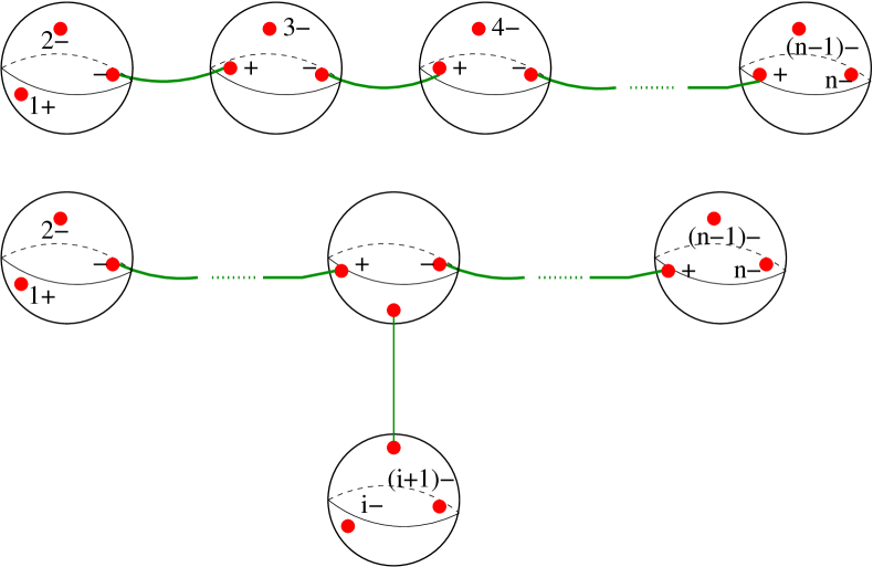
Figure 1: Two disconnected configurations contributing to $\mathcal{M}_{n}(1+,2-,\ldots,n-)$.

Each $CP^{1}$ represents a $(+,-,-)$ vertex, Fig. 2.

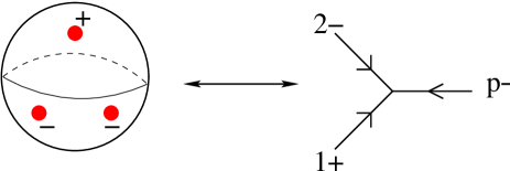
Figure 2: The $(+,-,-)$ graviton vertex.

This vertex is obtained by suitably extending the vanishing $(+,-,-)$ graviton amplitude off-shell. This is formally given by the square of the corresponding gluon amplitude [3]. The off-shell extension of the twistor $\lambda_{p}$ corresponding to an off-shell momentum $p$ has been given in [6] and amounts to defining

$$\lambda_{pa}=\frac{p_{a\dot{a}}\eta^{\dot{a}}}{[\tilde{\lambda}_{p},\eta]}$$ (3.1)

where $\eta^{\dot{a}}$ is an arbitrary spinor. The normalization factor is needed in order to have a consistent on-shell limit, and it can be dropped if the amplitude is homogeneous in the $\lambda_{p}$. The off-shell extension of the 3 graviton amplitude is therefore

$$\mathcal{M}_{3}=\left(\frac{\langle 2,p\rangle^{4}}{\langle 1,2\rangle\langle 2,p\rangle\langle p,1\rangle}\right)^{2}.$$ (3.2)

In this section we start focusing on $\mathcal{M}(1+,2-,3-,4-)$. This is computed using the MHV diagrams shown in Fig. 3.

Figure 3: The MHV diagrams contributing to the $\mathcal{M}(1+,2-,3-,4-)$ graviton amplitude.

Figure 4: Two of the fifteen MHV diagrams contributing to the $\mathcal{M}(1+,2-,3-,4-,5-)$ graviton amplitude.

The contribution of the first graph is given by

$$\frac{\langle 2p\rangle^{8}}{(\langle 12\rangle\langle 2p\rangle\langle p1\rangle)^{2}}\frac{1}{p^{2}}\frac{\langle 34\rangle^{8}}{(\langle p3\rangle\langle 34\rangle\langle 4p\rangle)^{2}}=\frac{\phi_{1}^{6}}{\phi_{2}^{2}\phi_{3}^{2}\phi_{4}^{2}}\frac{\langle 12\rangle\langle 34\rangle^{2}}{[12]}$$ (3.3)

where we have used $\lambda_{pa}=-\lambda_{1a}\phi_{1}-\lambda_{2a}\phi_{2}=\lambda_{3a}\phi_{3}+\lambda_{4a}\phi_{4}$, with $\phi_{i}=\tilde{\lambda}_{i\dot{a}}\eta^{\dot{a}}$. The remaining two diagrams are obtained by appropriately permuting the external labels. Using momentum conservation in the form of $\sum_{i=1}^{4}\langle yi\rangle[iz]=0$ (where $\lambda_{y}$ and $\tilde{\lambda}_{z}$ are arbitrary spinors), the final result can be arranged as

$$\mathcal{M}(1+,2-,3-,4-)=\frac{\phi_{1}^{6}}{\phi_{2}^{2}\phi_{3}^{2}\phi_{4}^{2}}\bigg{(}\langle 12\rangle\langle 34\rangle+\langle 13\rangle\langle 42\rangle+\langle 14\rangle\langle 23\rangle\bigg{)}\frac{\langle 42\rangle}{[13]}.$$ (3.4)

This vanishes by virtue of the Schouten identity $\langle ij\rangle\langle kl\rangle+\langle ik\rangle\langle lj\rangle+\langle il\rangle\langle jk\rangle=0$ which is valid for any four spinors.

Moving now to $\mathcal{M}(1+,2-,3-,4-,5-)$ we need to consider graphs of the type given in Fig. 4. The first diagram gives

$$\frac{\phi_{1}^{6}}{\phi_{2}^{2}\phi_{3}^{2}\phi_{4}^{2}\phi_{5}^{2}}\frac{\langle 12\rangle\langle 45\rangle(\langle 34\rangle\phi_{4}+\langle 35\rangle\phi_{5})^{6}}{[12][45](\langle 13\rangle\phi_{1}+\langle 23\rangle\phi_{2})^{4}}$$ (3.5)

where we have extended both $\lambda_{pa}$ and $\lambda_{qa}$ off-shell using the same spinor $\eta^{\dot{a}}$. This diagram yields 12 contributions once one takes into account all inequivalent exchanges of the negative helicity external gravitons. The second graph gives

$$\frac{\phi_{1}^{6}}{\phi_{2}^{2}\phi_{3}^{2}\phi_{4}^{2}\phi_{5}^{2}}\frac{\langle 23\rangle\langle 45\rangle(\langle 12\rangle\phi_{2}+\langle 13\rangle\phi_{3})^{4}}{[23][45](\langle 14\rangle\phi_{4}+\langle 15\rangle\phi_{5})^{2}}$$ (3.6)

and 2 other terms obtained by permutations. Imposing momentum conservation, with some computer assistance one can verify that the sum of the 12 contributions coming from (3.5) and the 3 contributions coming from (3.6) vanishes as expected.

We stress here the holomorphicity of (3.2), which is the only vertex appearing in this kind of graphs.

3.2 The googly amplitude

We now come to the investigation of disconnected contribution to $\mathcal{M}(1+,2+,3-,4-,5-)$. In the construction of the MHV graphs one also needs here the 4 graviton vertex depicted in Fig. 5.

Figure 5: The $(+,+,-,-)$ graviton vertex.

The expression for the 4 graviton amplitude was first obtained in [5] and is given by

$$\mathcal{M}(1+,2+,3-,q-)=\frac{\langle 3q\rangle^{8}}{\langle 12\rangle\langle 13\rangle\langle 1q\rangle\langle 23\rangle\langle 2q\rangle\langle 3q\rangle}\frac{[3q]}{\langle 12\rangle}.$$ (3.7)

One immediately notices that this expression is not holomorphic and this is in strong contrast with the 3 graviton vertex (3.2) and all the gluon MHV vertices. Naively, an off-shell extension of (3.7) would require a redefinition of $\tilde{\lambda}^{\dot{a}}$ whenever it appears in an internal line. Hermiticity suggests to take the complex conjugate of (3.1) so to have

$$\tilde{\lambda}_{p\dot{a}}=\frac{p_{a\dot{a}}\xi^{a}}{\langle\lambda_{p},\xi\rangle}$$ (3.8)

where $\xi=\eta^{*}$. Using this prescription one gets for the first graph in Fig. 6

$$\frac{\phi_{1}^{6}}{\phi_{3}^{2}}\frac{\langle 13\rangle\langle 45\rangle^{7}[45]}{\langle 25\rangle\langle 24\rangle[13](\langle 25\rangle\phi_{2}-\langle 54\rangle\phi_{4})(\langle 24\rangle\phi_{2}+\langle 54\rangle\phi_{4})(\langle 25\rangle\phi_{5}+\langle 24\rangle\phi_{4})^{2}}$$ (3.9)

and for the second graph

$$\frac{1}{\phi_{3}^{2}\phi_{4}^{2}(\phi_{3}\tilde{\phi_{3}}+\phi_{4}\tilde{\phi_{4}})}\frac{\langle 34\rangle(\langle 15\rangle\phi_{1}+\langle 25\rangle\phi_{2})^{7}([15]\tilde{\phi}_{1}+[25]\tilde{\phi}_{2})}{\langle 15\rangle\langle 25\rangle\langle 12\rangle^{2}[34](\langle 12\rangle\phi_{2}+\langle 15\rangle\phi_{5})(\langle 25\rangle\phi_{5}-\langle 12\rangle\phi_{1})}$$ (3.10)

where $\tilde{\phi}_{i}=\lambda_{ia}\xi^{a}$. The factor $\phi_{3}\tilde{\phi_{3}}+\phi_{4}\tilde{\phi_{4}}=[\tilde{\lambda}_{p},\eta]\langle\lambda_{p},\xi\rangle$ comes from the normalization of (3.1) and (3.8) which does not cancel in this case. One can get all the other seven graphs by permutation of the external labels as usual. The expected result for this amplitude is given in (2.6), which some computer algebra showed not to match with the one following from (3.9) and (3.10). Moreover, the result depends on $\eta$. Therefore the prescription seems to fail in this case. We are aware of the fact that the heuristic proof of covariance given in [6] might not be generalizable in the presence of non holomorphic vertices.

Figure 6: Two of the nine MHV diagrams contributing to the $\mathcal{M}(1+,2+,3-,4-,5-)$ graviton amplitude.

4 Conclusion

In this note we have explored the possibility of extrapolating the twistor construction of [1] to ordinary gravity. We have checked that the simplest non-trivial gravity quantity, namely the 5 graviton googly amplitude, confirms the expectations of [1] and is indeed supported on a connected degree 2 curve in twistor space, just as the corresponding amplitude in the gauge theory . There are however important differences between the two. In the simplest, MHV case, these stem from the fact that gravity amplitudes contain extra delta-function derivatives in twistor space variables, or equivalently they are not holomorphic in Minkowski space variables. It is clearly desirable to confirm that such behavior persists for further, non MHV graviton amplitudes.

In a complementary approach to the computation presented in Section 2, we have further tried calculating tree-level graviton amplitudes by using MHV subamplitudes as vertices (computed from the gauge theory quantities by using the KLT relations, and suitably continuing them off-shell), in the spirit of the prescription given in [6] for gauge theories. Although it is possible that such a generalization might be feasible in principle, it is clear from our results that novel ingredients are necessary to correctly reproduce non-trivial gravity amplitudes.

We nevertheless consider it encouraging that the $(+,-,-,-)$ and $(+,-,-,-,-)$ graviton amplitudes vanish when computed from MHV vertices. We are aware that these are very special cases. Indeed, $(+,-,\ldots,-)$ amplitudes involve only trivalent MHV vertices, which are holomorphic even in the graviton case. Unfortunately, the four-valent graviton MHV vertex is not holomorphic. We believe that this non-holomorphicity is an important reason for the failure of the MHV prescription to correctly reproduce the 5 graviton googly amplitude discussed in this note.

We must emphasize that the twistor string theory underlying an eventually successful version of such a construction might have nothing to do with the one of [1], or even there might be no such theory at all. Indeed, the closed string sector of the model of [1] is expected to be a kind of instanton expansion around ${\cal N}=4$ self-dual superconformal gravity. General Relativity is most definitely not conformally invariant, and therefore it should be related to a different model. The computation in Section 2 seems to suggest that there could be some localization in twistor space, and the disconnected prescription could provide an explicit and computable “instanton” expansion around some “self-dual” theory. In this respect, we think that the non-holomorphicity of higher MHV vertices could provide a hint about which could be the right theory to expand around.

Acknowledgments

We would like to thank Zvi Bern, Freddy Cachazo, Martin Roček, and Warren Siegel for helpful discussions. The research of R.R. and D.R.-L. is partially supported by NSF Grant No. PHY0098527.

References

- [1] E. Witten, Perturbative Gauge Theory as a String Theory in Twistor Space, arXiv:hep-th/0312171.
- [2] S. Parke and T. Taylor, An Amplitude for N Gluon Scattering, Phys. Rev. Lett. 56 (1986) 2459; F. A. Berends and W. T. Giele, Recursive Calculations for Processes with N Gluons, Nucl. Phys. B306 (1988) 759.
- [3] H. Kawai, D. C. Lewellen and S. H. Tye, A Relation between Tree Amplitudes of Closed and Open Strings, Nucl. Phys. B269 (1986) 1.
- [4] Z. Bern, Perturbative Quantum Gravity and its Relation to Gauge Theory, arXiv:gr-qc/0206071.
- [5] F. A. Berends, W. T. Giele and H. Kuijf, On Relations between Multi-gluon and Multi-graviton Scattering, Phys. Lett. B211 (1988) 91.
- [6] F. Cachazo, P. Svrcek and E. Witten, MHV Vertices and Tree Amplitudes in Gauge Theory, arXiv:hep-th/0403047.
- [7] E. Witten, Parity Invariance for Strings in Twistor Space, arXiv:hep-th/0403199.
- [8] R. Roiban, M. Spradlin and A. Volovich, A Googly Amplitude from the B-model in Twistor Space, arXiv:hep-th/0402016; R. Roiban and A. Volovich, All Googly Amplitudes from the B-model in Twistor Space, arXiv:hep-th/0402121; R. Roiban, M. Spradlin and A. Volovich, On the Tree-level S-Matrix of Yang-Mills Theory, arXiv:hep-th/0403190.
- [9] N. Berkovits, An Alternative String Theory in Twistor Space for Super Yang-Mills, arXiv:hep-th/0402045; N. Berkovits and L. Motl, Cubic Twistorial String Field Theory, arXiv:hep-th/0403187.
- [10] A. Neitzke and C. Vafa, Strings and the Twistorial Calabi-Yau, arXiv:hep-th/0402128; N. Nekrasov, H. Ooguri and C. Vafa, S-duality and Topological Strings, arXiv:hep-th/0403167; M. Aganagic and C. Vafa, Mirror Symmetry and Supermanifolds, arXiv:hep-th/0403192.
- [11] S. Gukov, L. Motl and A. Neitzke, Equivalence of Twistor Prescriptions for Super Yang-Mills, arXiv:hep-th/0404085.
- [12] C.-J. Zhu, The Googly Amplitudes in Gauge Theory, arXiv:hep-th/0403115.
- [13] G. Georgiou and V. V. Khoze, Tree Amplitudes in Gauge Theory as Scalar MHV Diagrams, arXiv:hep-th/0404072.
- [14] W. Siegel, Untwisting the Twistor Superstring, arXiv:hep-th/0404255.
- [15] D. A. Kosower, Light Cone Recurrence Relations for QCD Amplitudes, Nucl. Phys. B335 (1990) 23.