Dynamics of Q-Balls in an expanding universe

Abstract

We analyse the evolution of light Q-balls in a cosmological background, and find a number of interesting features. For Q-balls formed with a size comparable to the Hubble radius, we demonstrate that there is no charge radiation, and that the Q-ball maintains a constant physical radius. Large expansion rates cause charge migration to the surface of the Q-ball, corresponding to a non-homogeneous internal rotation frequency. We argue that this is an important phenomenon as it leads to a large surface charge and possible fragmentation of the Q-ball. We also explore the deviation of the Q-ball profile function from the static case. By introducing a parameter $\epsilon$, which is the ratio of the Hubble parameter to the frequency of oscillation of the Q-ball field, and using solutions to an analytically approximated equation for the profile function, we determine the dependence of the new features on the expansion rate. This allows us to gain an understanding of when they should be considered and when they can be neglected, thereby placing restrictions on the existence of homogeneous Q-balls in expanding backgrounds.

I Introduction

Q-balls kn:coleman are non-topological solitons that exist as minimum energy configurations of a complex scalar field (typically a flat direction in a MSSM model kn:kusenko ; kn:shaposhnikov ; kn:mcdonald ) with a global U(1) symmetry; the gauged version has been studied in kn:lee . First introduced by Coleman kn:coleman , following pioneering work by Friedberg, Lee and Sirlin kn:friedberg , their formation, particularly through an Affleck-Dine condensate collapse khlebnikov ; kn:enqvist ; kn:kawasaki , has been frequently investigated . However, little work has gone into looking at the behaviour of general fully formed Q-balls in a cosmological background. The need to do this is becoming increasingly important as Q-balls are often discussed in a cosmological context, typically as a possible catalyst for baryogenesis kn:mcdonald and as candidates for dark matter kn:steinhardt ; kn:shaposhnikov . In this short paper we begin this investigation by considering light Q-balls (where the Q-ball energy density is dominated by the background energy density) in a cosmological setting.

The background expansion leads to changes in the Q-ball behaviour from the static case. We identify a parameter $\epsilon$, which is the ratio of the Q-ball oscillation frequency (in the core of the Q-ball) and the Hubble parameter, as a measure of the deviation from static background solutions. We then show that in an expanding background the Q-ball characteristics are determined by $\epsilon$. By numerically obtaining the explicit relation between $\epsilon$ and the deviations from the static solutions, we are able to answer two important questions: when should we be considering background expansion effects and how do these effects depend on the rate of expansion? Turning explicitly to the effect of the expansion on the Q-ball we show that the Q-ball parameters exhibit expansion driven oscillations and that the expansion causes the field rotation frequency to become non-homogeneous, driving the conserved charge to the surface of the Q-ball but not radiating it, whilst maintaining a constant physical radius. In what follows, we begin by summarising the basics of Q-balls in flat space leading to a discussion of the problems a dynamic background introduces and our proposed way of analysing the new solutions. In section III we numerically solve the full system of a light Q-ball in an expanding Universe, and explicitly demonstrate the consistency of introducing the parameter $\epsilon$. We introduce our analytic approach in section IV and discuss its uses and implications in section V. We summarise our results in section VI.

II Q-balls in an expanding background

The evolution of a complex scalar field $\varphi$ with a Lagrangian density ${\cal L}=\left|\partial\varphi\right|^{2}-V(|\varphi|^{2})$ is given by

$$\Box\varphi=\frac{\partial V}{\partial\varphi^{*}}.$$ (2.1)

For a spherically symmetric field of the form $\varphi=e^{i\omega t}f(r)$, where the frequency $\omega$ and profile function $f$ are real, in a flat background we have

$$\nabla^{2}f+\frac{\partial V_{eff}}{\partial f}=0,$$ (2.2)

where $V_{eff}=\frac{1}{2}\omega^{2}f^{2}-\frac{1}{2}V(f^{2})$. Equation (2.2) is equivalent to Newtonian motion, with a time dependent friction term, of a particle in a potential $V_{eff}$, with r acting as time. A Q-ball corresponds to a solution where the particle starts at some point $\varphi_{0}\equiv\varphi(r=0)$ and rolls down the potential coming to rest at the origin. This would be a field configuration with $\varphi\rightarrow 0$ as $r\rightarrow\infty$, a necessary condition for finite energy, if we require $V(0)=0$. The conditions for such a solution to exist are that $V_{eff}$ is decreasing near the origin (allowing the particle to slow down and come to rest there) and that at the starting point $V_{eff}\left(\left|\varphi_{0}\right|^{2}\right)\geq 0$, so the particle has enough energy to reach $\varphi=0$. Hence for a flat space Q-ball solution to exist, the value of $\omega$ is restricted to be in the range

$$\frac{2V\left(\left|\varphi_{0}\right|^{2}\right)}{\left|\varphi_{0}\right|^{2}}\leq\omega^{2}\leq V^{\prime\prime}(0).$$ (2.3)

Assuming appropriate values of $\omega$ are found, then equation (2.2) has an exact soliton (Q-ball) solution with a stabilising (against decay) Noether charge given by kn:coleman

$$Q=\omega\int|\varphi|^{2}d^{3}x.$$ (2.4)

In a Robertson-Walker universe with scale factor $a(t)$, the equation of motion becomes

$$\frac{1}{a^{2}}\left(\nabla^{2}\varphi\right)-\frac{\partial^{2}\varphi}{\partial t^{2}}-\frac{3}{a}\left(\frac{\partial a}{\partial t}\right)\left(\frac{\partial\varphi}{\partial t}\right)=\frac{\partial V}{\partial\varphi^{*}}.$$ (2.5)

In this case the ansatz $\varphi=e^{i\omega t}f(r)$ with constant $\omega$ is no longer a solution and so the flat space Q-ball scenario of a spherically symmetric field configuration with a constant internal rotation frequency does not hold. Now, in most cosmological settings we may neglect the Hubble drag term as a first approximation, however a better and more instructive approach is to keep all the terms and simply work in conformal time $\eta$ defined by $dt=a(\eta)d\eta$. Introducing $\phi=\varphi a(\eta)$ we obtain the following evolution equation

$$\nabla^{2}\phi-\phi^{\prime\prime}=a^{4}\frac{\partial}{\partial\phi^{*}}V(|\phi|^{2}/a^{2})-\left(\frac{a^{\prime\prime}}{a}\right)\phi$$ (2.6)

where time derivatives with respect to $\eta$ are denoted by a prime. The utility of this approach is that all the time dependence of the background has been re-written as a time dependent potential for $\phi$, ${\cal V}(|\phi|^{2})=a^{4}V(|\phi|^{2}/a^{2})-(a^{\prime\prime}/a)|\phi|^{2}$.

III Numerical simulations

For our analytic approach in section IV we introduce a small parameter $\epsilon=H/\omega_{0}$, so for our purposes a natural background for looking at the evolution of the Q-ball profile is de-Sitter space. In this case the parameter $\epsilon$ is a constant and so by looking at the profile evolution over a constant range of the scale-factor (constant number of efoldings), but at different rates of expansion, we can explore the dependence of the approximation on $\epsilon$. First of all though we shall perform simulations of the full evolution, (2.6), so we can later test our analytic method. In our simulations we used a form of the potential motivated from supersymmetry, namely

$$V(\varphi)=\alpha\varphi^{2}-\beta\varphi^{4}+\gamma\varphi^{6}$$ (3.7)

with $\alpha=2.3\times 10^{7}{\rm GeV}^{2}$, $\beta=1.0$, and $\gamma=1.0\times 10^{-8}{\rm GeV}^{-2}$. The chosen values correspond to the small field expansion of a SUSY potential of the form $V(\varphi)=M^{4}\ln(1+\varphi^{2}/M^{2})$ where $M\sim 10^{4}$ GEV is the scale of SUSY breaking. Recall that we are considering light Q-balls, defined as those whose dynamics are determined by the background spacetime, and whose own contribution to the energy density in the Friedmann equation is negligible. Given that, we choose an appropriately large value $H\sim 10^{2}$ GeV for the Hubble parameter. This corresponds to a background energy scale of $10^{10}$ GeV, or an evolution in the radiation dominated era, just after say reheating at the end of a period of early Universe inflation. In order to test the robustness of the parameter $\epsilon$ in determining the true solution, we ran a series of simulations in which we fixed the charge of the Q-ball and varied $H$, increasing it from a starting value of $100$GeV. We verified our results for a number of values of Q but the results we show here correspond to Q=300, (giving $\epsilon=0.05$ for $H=100$GeV).

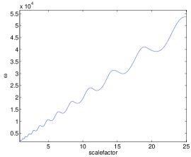
Figure 1: Figure showing $\omega$ in the core of the Q-ball as a function of the scalefactor.

Starting with the profile of a static configuration, we obtained the evolution of the Q-ball as we turned on the expansion of the universe, reaching a de-Sitter background by $a=1$. We then evolved the profile with this background and a fixed value of $\epsilon$ for $\ln(25)$ efoldings. This was repeated for different values of $\epsilon$. Throughout the evolution we found that the Q-ball charge (defined by the Noether charge $-4\pi i\int dr\;r^{2}\left[\phi^{*}\phi^{\prime}-\left(\phi^{\prime}\right)^{*}\phi\right]$ where r is the comoving radial coordinate) was conserved. So the expansion did not lead to leakage of charge.

Numerically the internal rotation frequency (in comoving units) was defined as

$$\omega(r)\equiv Im\left[\frac{\phi^{\prime}(r)}{\phi(r)}\right]$$ (3.8)

and we observed that for slow expansion rates its value at the core of the Q-ball exhibited oscillatory behaviour about a general evolution where it remained proportional to $a$ as shown in Fig. 1. Similarly, the profile amplitude $\phi$ also uniformally increased as $a$ whereas the Q-ball co-moving radius $R$ decreased proportionally to $a^{-1}$. Recalling the definition of $\phi=\varphi a$, we see that the physical Q-ball parameters (radius and amplitude $\varphi$) oscillate about constant values. The main deviation from a flat space Q-ball arose through the non-homogeneity of $\omega(r)$, which emerged as $\epsilon$ increased. Recalling that for homogeneous rotation frequencies the charge distribution is proportional to the amplitude of the profile function, and that no major change to the profile shape was observed, such a non-homogeneous $\omega$ leads to a new charge density distribution. This is evident in Fig. 2 which shows how the expansion (with $\epsilon=0.25$) causes charge to move towards the surface of the Q-ball as opposed to the case of a typical charge distribution in a static background indicated by the inset figure shown. However, once established, the charge density profile did not vary with the expansion. The oscillations of the Q-ball parameters are to be expected in an expanding background; they correspond to oscillations about the minimum energy configuration of the Q-ball and are driven by the expansion of the universe. To see this, recall that the expansion leads to time-varying potentials, in which the minimum is varying with time, whilst the field is oscillating about the minimum.

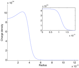
Figure 2: Figure showing the charge density radial dependence for a profile in an expanding background ($\epsilon$=0.25), with the inset showing a typical static background profile. Note how the expansion causes the charge to move towards the surface of the Q-ball, compared to the static case.

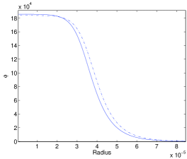
Figure 3: Figure showing the numerical end profile (solid line) and the approximated profile (dotted line) obtained from the static solution for the case $\epsilon=0.1$.

IV Analytic approach

The usefulness of adopting conformal time emerges because (2.6) looks like (2.2) but with a time varying potential. It is natural, therefore, to make the approximation that a Q-ball profile at a particular time is given by solving (2.6) at that time, $\phi=e^{i\omega\eta}f(r)$, leading to

$$\nabla^{2}f+\frac{\partial}{\partial f}\left(\frac{1}{2}\omega^{2}f^{2}+\frac{1}{2}\frac{a^{\prime\prime}}{a}f^{2}-\frac{1}{2}a^{4}V(f)\right)=0.$$ (4.9)

This equation is of the same form as the flat space equation (2.2), but the price we pay is the introduction of a new time dependent effective potential. At a particular moment in time, equation (4.9) has soliton solutions with the same constraints as the flat space case, but these are Q-ball solutions in a dynamic background. This is an appealing result; we can think of Q-balls in a dynamic background as flat space Q-balls with a time varying potential. It is clear that our approximate ansatz is not an exact solution as the amplitude has no time dependence to match the evolving time dependent potential. Solving for static profiles at different values of $a$ and $a^{\prime\prime}$ provides an approximation for the evolving profile. Equation (2.5) approaches the flat space case in the limit $\frac{H}{\omega}\rightarrow 0$. Therefore we parameterise our approximation by the adiabatic parameter $\epsilon=\frac{H}{\omega_{0}}$ where $H$ is the Hubble parameter and $\omega_{0}$ is the frequency in the core of the Q-ball at the initial scalefactor value. We now show that we can closely predict the evolving profile of the true solution, based on the corresponding static solution. And that deviations from the static solutions are characterised by $\epsilon$.

We would like to establish how in an expanding background the deviations observed from the static profiles, depend on $\epsilon$. It is straightforward to solve for a static profile with the same overall charge as the exact solution and at the corresponding values of $a$ and $a^{\prime\prime}$. Having done this we obtain an adiabatic approximation to the evolved profile, which can be compared with the true solution. As an example of the strength of the approximation for say $\epsilon=0.1$, Fig. 3 shows an overlap of the true final profile (solid line) and the corresponding ‘static’ approximation (dotted line); they show good agreement. To quantify the accuracy of the approximation we introduce the parameter

$$\chi=1-\frac{\left|\int\phi_{A}^{*}\phi_{N}\right|^{2}}{\int\left|\phi_{A}\right|^{2}\int\left|\phi_{N}\right|^{2}}\geq 0,$$ (4.10)

where $\phi_{N}(r)$ is the numerically evolved profile and $\phi_{A}(r)$ is the adiabatic approximation. Note that $\chi$ measures how the profiles differ including the phases of the profiles, so such measurements would include effects from non-homogeneous rotation frequencies. Calculating $\chi$ throughout the evolution we find that it exhibits oscillations of the same nature as those found in the Q-ball parameters. Averaging over these oscillations gives us a parameter $\chi_{ave}$ as a measure of how well the adiabatic approximation holds as a function of $\epsilon$. Figure 4 shows a plot of $\ln\chi_{\rm ave}$ against $\frac{1}{\epsilon}$, with error bars corresponding to the standard deviation of the oscillations from the mean (note that these are not errors in the value of $\chi_{ave}$ but are there to show the scale of the oscillations). We see that there is a negative logarithmic correlation meaning that the adiabatic approximation rapidly improves with decreasing $\epsilon$.

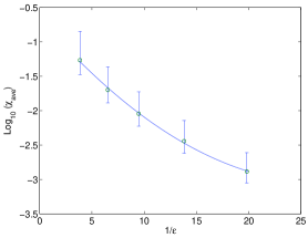
Figure 4: Figure showing $\ln\chi_{\rm ave}$ as a function of $\frac{1}{\epsilon}$.

Figure 4 helps us to understand when we should consider expansion effects in Q-ball dynamics and how they vary with $\epsilon$ in that it provides direct information on how the expansion affects the profile. For example, for expansion rates of $\epsilon=0.2$ we already have deviations in the profiles corresponding to around 10%, whereas for $\epsilon=0.05$ these reduce to a negligible value of 0.1%. There is another useful non-trivial aspect to Figure 4. We, of course, expect that as $\epsilon\rightarrow 0$, we recover the static solution. However, an important question is how rapidly do we approach it? We can see that the deviation from the static Q-balls depend on high powers of $\epsilon$. Such a strong, highly non-linear, dependence is difficult is derive analytically and it provides important information in a cosmological setting where $\epsilon$ is varying. We have shown that as long as the parameter $\epsilon$ remains small enough, then there is a good adiabatic approximation describing the evolution of a Q-ball in an expanding background. In fact from the definition $\epsilon=H/\omega_{0}$, we see that this decreases with time in any universe with dominating fluid whose equation of state $\omega_{\rm dom}>-1$ (note this is not the same $\omega$ as defining the Q-ball). Hence in a matter and radiation dominated universe the adiabatic approximation improves with time.

V The approximation and its limits

Using the change of variables we have introduced it is possible to analytically consider the behaviour of a Q-ball in a slowly expanding background. Let us analyse the approximations we have made in more detail. Consider the general potential given in equations (4.9) and (3.7). This leads to an effective potential given by

$$V_{eff}=\frac{1}{2}\left(-\alpha a^{2}+\frac{a^{\prime\prime}}{a}+\omega^{2}\right)\phi^{2}+\frac{1}{2}\beta\phi^{4}-\frac{1}{2}\frac{\gamma}{a^{2}}\phi^{6}.$$ (5.11)

An adiabatic evolution allows us to solve for Q-ball properties using (5.11) and treating the scalefactor as a constant. Recalling the constraints arising in equation (2.3) for a static flat space solution, we can obtain instantaneous constraints for the expanding Universe case:

$$\alpha a^{2}-\frac{\beta^{2}a^{2}}{4\gamma}-\frac{a^{\prime\prime}}{a}\equiv\omega_{\rm min}^{2}\leq\omega^{2}\leq\omega_{\rm max}^{2}\equiv\alpha a^{2}-\frac{a^{\prime\prime}}{a}.$$ (5.12)

We can also derive the scalefactor dependence of the Q-ball parameters. For example, using standard thin wall limit arguments kn:coleman77 we have the expression for the core field amplitude

$$|\phi_{0}|^{2}\rightarrow a^{2}\frac{\beta}{2\gamma}$$ (5.13)

and for the Q-ball radius

$$R\sim a\frac{\beta}{2\sqrt{\gamma}}\frac{1}{\Delta\omega^{2}}+\frac{1}{\sqrt{\Delta\omega^{2}}}.$$ (5.14)

where $\Delta\omega^{2}=\omega^{2}-\omega_{\rm min}^{2}$. By introducing the dimensionless parameter

$$\zeta=\frac{4\gamma}{\beta^{2}a^{2}}\Delta\omega^{2},$$ (5.15)

with the range $0<\zeta\leq 1$ we can write this as

$$R\sim\frac{2\sqrt{\gamma}}{a\beta}\left(\frac{1}{\zeta}+\frac{1}{\sqrt{\zeta}}\right).$$ (5.16)

We see that these expressions, derived by considering the equations at a particular time, correctly predict the dependence of the parameters on the scalefactor. Similar calculations can be used to predict the background dependence of other, more complicated parameters. It is encouraging that the analytic estimates arising from the use of the adiabatic parameter $\epsilon$, and the thin wall approximation lead to the correct values for the actual Q-ball parameters. Of course, as $\epsilon$ increases, the validity of the analytic result comes into question, eventually breaking down for large enough expansion rates. Fortunately though, it appears to hold well for a wide range of cosmologically interesting parameters. The breakdown of the approximation can be seen through the inhomogeneous charge distribution which emerges as $\epsilon$ increases as seen in figure (2). These type of Q-balls are very interesting in themselves as they differ from the Q-balls discussed in kn:coleman with a homogeneous rotation frequency distribution. In fact for significant expansion rates, they can evade the bounds imposed in (5.12), which correspond to (2.3). However, the bounds of (5.12) do give us background dependent constraints on the existence of nearly - homogeneous-$\omega$ Q-balls.

VI Conclusions

In this paper we have analysed Q-ball solutions in an expanding background. As expected, the presence of expansion changes the solution from the traditional form obtained in a Minkowski background, namely those which are spherically symmetric and have a constant homogeneous frequency of rotation. However, by solving the system in conformal time, we can rewrite the equations of motion for the Q-ball in an expanding background in such a way that it mimics the case of the static background, the only difference being that the effective potential for the Q-ball given in equation (5.11) becomes explicitly time dependent as a result of the scale factor. This then allows us to introduce an adiabatic parameter $\epsilon=\frac{H}{\omega_{0}}$ with which to analyse solutions to the full equations of motion. The smaller $\epsilon$ is, the closer the evolution is to the original static spacetime case. Explicit calculations of the deviations from static profiles, seen in Fig. 4, give us their dependence on $\epsilon$. This is important information when considering Q-balls in a cosmological context. Recalling that $\epsilon$ is a function of both the expansion rate and the rotation frequency we see that in backgrounds where these effects play a role, even small variations in the frequency or the expansion rate can cause movement of charge. We numerically showed that Q-balls existing in an expanding background conserved their charge, maintained a constant radius, whilst exhibiting oscillations in their frequency, a reflection of the dependence on the expansion of the universe. The analytic approximations we developed are able to recover the background dependence of these features as seen through equations (5.13) and (5.16). We are also able to place background dependent constraints on the existence of Q-balls with homogeneous rotation frequencies(5.12).

We have noticed in the simulations that the Q-ball solutions, whilst still existing in that they conserve their charge, now develop an inhomogeneous charge distribution (see figure (2)). Further study of the configurations could include predicting the general form of the charge density profile as a function of the background expansion. Given that the Q-ball charge profile is dependent on the expansion rate in a way which drives charge to the surface, we would anticipate that for large enough $\epsilon$, the charge is confined to the surface of the Q-ball. Such a configuration is unstable due to a large surface tension (defined by a positive energy-charge relation) and no bulk tension to hold it together. A similar situation for the case of non-topological cosmic strings is discussed in copeland and the same conclusions are reached. Any cosmological considerations of Q-balls where the oscillation frequency is of the order of the Hubble parameter should include discussions of stability against this kind of effect. This is particularly important in the early universe where we are dealing with rapid expansion rates.

- (1) S. R. Coleman, Nucl. Phys. B 262, 263 (1985)
- (2) A. Kusenko, Nucl. Phys. Proc. Suppl. 62A/C, 248 (1998) [arXiv:hep-ph/9707306].
- (3) A. Kusenko and M. E. Shaposhnikov, Phys. Lett. B 418, 46 (1998) [arXiv:hep-ph/9709492].
- (4) K. Enqvist and J. McDonald, Phys. Lett. B 425, 309 (1998) [arXiv:hep-ph/9711514].
- (5) K. M. Lee, J. A. Stein-Schabes, R. Watkins and L. M. Widrow, Phys. Rev. D 39 (1989) 1665.
- (6) R. Friedberg, T. D. Lee and A. Sirlin, Phys. Rev. D 13 (1976) 2739.
- (7) S. Khlebnikov and I. Tkachev Phys. Rev. D 61 (2000) 083517 [arXiv:hep-ph/9902272].
- (8) K. Enqvist and J. McDonald, Nucl. Phys. B 570, 407 (2000) [arXiv:hep-ph/9908316].
- (9) S. Kasuya and M. Kawasaki, Phys. Rev. D 61, 041301 (2000) [arXiv:hep-ph/9909509].
- (10) A. Kusenko and P. J. Steinhardt, Phys. Rev. Lett. 87, 141301 (2001) [arXiv:astro-ph/0106008]. kn:coleman77
- (11) S. R. Coleman, Phys. Rev. D 15 (1977) 2929 [Erratum-ibid. D 16 (1977) 1248].
- (12) E. J. Copeland, E. W. Kolb and K. M. Lee Phys. Rev. D 38, 3023 (1988).