May 2004

KUNS-1914

RIKEN-TH-24

UTHEP-488

hep-th/0405076

1 Introduction

It is now widely recognized that the nonperturbative effect in string theory that behaves as $\sim e^{-\frac{1}{g_{s}}}$ [1] stems from the dynamical hypersurfaces in space-time (the D-brane) on which open strings can end [2]. The double scaling limit of matrix models [3, 4] may enable us to learn more about this, at least for noncritical strings. It was realized in the early 1990s that the string equation (Painlevé equation) indeed inherits such nonperturbative effects [5, 6]; they correspond to the deviation of its solutions from the genus expansion of two-dimensional gravity. In the early 2000s, studies of the D-brane have been developed from the viewpoint of Liouville field theory [7, 8, 9].

Given this situation, we are tempted to reinvestigate nonperturbative effects of the noncritical string theory in full detail. In particular, we would like to ask if nonperturbative effects introduce a continuous parameter characterizing vacua like the $\theta$ parameter in QCD, or if they are fully calculable as an intrinsic property of the matrix model.

We focus on the $c=0$ noncritical string here in order to address the above questions as clearly as possible. First, let us recall the nonperturbative effects observed in string equation, following Refs. [5] and [6]. The variable for which to solve is the specific heat $u(t)$, depending on the renormalized cosmological constant $t$. The string equation with respect to it takes the form of Painlevé equation I,

$$u^{2}+\frac{g_{s}^{2}}{6}\,\partial_{t}^{2}u=t\,.$$ (1.1)

The leading-order contribution to $u(t)$ in the genus expansion is $(g_{s})^{0}$, and it is related to the free energy $F$ ($F\equiv{\rm ln}\,Z$ with the matrix model partition function $Z$) through

$$u=g_{s}^{2}\,\partial_{t}^{2}F\,.$$ (1.2)

$u(t)$ admits a perturbative series expansion:

$$u_{\rm pert}(t)=-\sqrt{t}+\frac{1}{48}\,\frac{g_{s}^{2}}{t^{2}}+\frac{49}{4608}\,\frac{g_{s}^{4}}{t^{\frac{9}{2}}}+\cdots\,.$$ (1.3)

However, there may be some degree of ambiguity in the above solution, due to nonperturbative effects. To examine this point, let us suppose that there is another solution $u(t)$ infinitesimally close to the above perturbative solution, which we write

$$u(t)=u_{\rm pert}(t)+\Delta u(t)\,.$$ (1.4)

Then, if we write $\Delta u(t)$ in the form

$$\Delta u(t)=A\,e^{-\frac{h(t)}{g_{s}}}\,,$$ (1.5)

the equation for $h(t)$ admits an expansion with respect to $g_{s}$,

$$\left((\partial_{t}h(t))^{2}-12\sqrt{t}+Ae^{-\frac{h(t)}{g_{s}}}\right)+g_{s}\left(-\partial_{t}^{2}h(t)\right)+{\cal O}(g_{s}^{2})=0\,.$$ (1.6)

Noting that $e^{-\frac{h(t)}{g_{s}}}$ is negligible as long as $g_{s}$ is small, $h(t)$ can be solved as

$$h(t)=\frac{8\sqrt{3}}{5}\,t^{\frac{5}{4}}+\frac{g_{s}}{8}\,{\rm ln}\,t+{\cal O}(g_{s}^{2})\,.$$ (1.7)

By inserting this into Eqs. (1.5) and (1.4) and integrating $u(t)$ twice over $t$, the free energy $F$ is found as

$$F=F_{\rm pert}+F_{\rm inst}\,,$$

$$F_{\rm pert}=-\frac{4}{15}\,\frac{t^{\frac{5}{2}}}{g_{s}^{2}}-\frac{1}{48}\,{\rm ln}\,t+\frac{7}{5760}\,\frac{g_{s}^{2}}{t^{\frac{5}{2}}}+{\cal O}(g_{s}^{4})\,,$$

$$F_{\rm inst}=\frac{C}{t^{\frac{5}{8}}}\,\exp\left[-\frac{8\sqrt{3}}{5g_{s}}\,t^{\frac{5}{4}}\right]\left(1+{\cal O}(g_{s})\right)\,.$$ (1.8)

Here, $F_{\rm inst}$ is the non-perturbative contribution to the free energy, which can be interpreted as an instanton effect [5, 2]. Recent developments have identified the origin of these effects as D-branes [10, 11, 12, 13, 14]. However, the overall factor of $C$ for the instanton contribution cannot be determined from the string equation (1.1) itself; it is a constant of integration that should be determined from the other boundary condition mentioned above. That is, the string equation determines the D-instanton action

$$S_{\rm inst}=\frac{8\sqrt{3}}{5g_{s}}t^{\frac{5}{4}}$$ (1.9)

uniquely, and it shows that the D-instanton contributes to the free energy in the form

$$\frac{C}{t^{\frac{5}{8}}}\,e^{-S_{\rm inst}}\,.$$ (1.10)

However, the weight $C$ relative to the perturbative contribution, which corresponds to the chemical potential needed to bring a D-instanton into the system, remains undetermined with the string equation (1.1).

Our main focus here is concerned with the chemical potential of the D-instanton. There are the following two possibilities for $C$:

(a)

$C$ is a parameter characterizing the vacua as a result of quantizing the system, like the $\theta$-parameter in QCD. Specifically, each value of $C$ corresponds to a distinct vacuum.

(b)

$C$ is calculable and its value is uniquely determined. In this sense, the string equation does not fully describe the properties of the system.

We are able to determine which possibility is actually realized by inquiring whether the chemical potential of the instanton can be calculated directly by carrying out the path integral of the $c=0$ matrix model.

Our main result here is the following: The value of $C$ can be calculated. Moreover, $C$ does not depend on the details of the matrix model action, and it is thus a universal quantity, given by

$$C=i\,\frac{1}{8\cdot 3^{\frac{3}{4}}\cdot\sqrt{\pi}}\,.$$ (1.11)

Reflecting the instability of the vacuum in the presence of a D-instanton, $C$ is a purely imaginary number. Our result shows that the lifetime of such a vacuum is uniquely determined and does not depend on the regularization scheme. These results indicate that assertion (b) is correct.

This paper is organized as follows. We start in §2 by identifying the instanton effect in the matrix model and showing that it corresponds to the D-instanton effect in $c=0$ Liouville field theory. Then, we divide the partition function of the matrix model into the sum of contributions $Z^{(n\text{-inst})}$ from $n$ of instantons ($n=0,\,1,\,\cdots$) by restricting the integration regions of the eigenvalues in a proper way. There, we also derive various significant equations for estimating the chemical potential $\mu$ of an instanton, i.e., the ratio of the single-instanton contribution $Z^{(1\text{-inst})}$ to the trivial vacuum contribution $Z^{(0\text{-inst})}$,

$$\mu\equiv\frac{Z^{(1\text{-inst})}}{Z^{(0\text{-inst})}}\,.$$ (1.12)

In §3, we apply the expression obtained in §2 to the estimation of the chemical potential of an instanton, with the help of the orthogonal polynomial method. We find that the chemical potential of an instanton is indeed given by the value in Eq. (1.11).

Section 4 constitutes the second part of the paper. Then, we reconsider the result obtained in the previous sections from the matrix model calculation by examining the loop equations more closely. First, we consider the loop amplitude in the background produced by single-instanton. This is done by taking the expectation value of the loop amplitude after restricting ourselves to single-instanton sector a priori, ignoring the other sectors. We find that the loop equations in the large $N$ limit determine the loop amplitude in the single-instanton sector, up to a constant factor. In order to determine this constant, we need the loop equations at all orders.

Next, we examine whether the loop equations determine the chemical potential of an instanton. As seen in §3, the chemical potential of an instanton is universal. However, it requires regularization of a divergence of type ${\rm ln}\,N$. Thus, we find that the loop equations obtained after taking the continuum limit cannot determine the chemical potential of an instanton. This fact indicates that it is quite difficult in string theory with closed strings only to fully describe the nonperturbative effects of strings, and that open strings or matrices should be regarded as fundamental degrees of freedom. Section 5 contains the conclusion of this paper.

2 The instanton in $c=0$ noncritical string theory

In this section, we show that the instanton in the one-matrix model is identical to the D-instanton in the $c=0$ noncritical string theory and that it indeed gives the nonperturbative effect discussed in the introduction.

2.1 Action of the instanton

As a concrete example, we consider the one-matrix model with a cubic potential,

$$S=N{\rm tr}V(\phi),\hskip 28.45274ptV(x)=\frac{1}{2}\phi^{2}-\frac{g}{3}\phi^{3},$$ (2.1)

where $\phi$ is an $N\times N$ Hermitian matrix. The effective action for the eigenvalues $\lambda_{i}$ ($i=1,\cdots,N$) is given by

$$S_{{\rm eff}}=-\sum_{i<j}\log(\lambda_{i}-\lambda_{j})^{2}+N\sum_{i}V(\lambda_{i}).$$ (2.2)

Hereafter, we consider the situation in which a single eigenvalue ($\lambda_{N}$) is separated from the others. Then, the partition function of the matrix model (2.1) is expressed as

$$Z_{N} = \int dx\int d\lambda_{1}\cdots d\lambda_{N-1}\left(\prod_{i=1}^{N-1}(x-\lambda_{i})^{2}\right)\Delta^{(N-1)}(\lambda_{1},\cdots,\lambda_{N-1})^{2}$$ (2.3)

$$\times e^{-N\sum_{i=1}^{N-1}V(\lambda_{i})}e^{-NV(x)},$$

where $x$ denotes $\lambda_{N}$, and $\Delta^{(N-1)}(\lambda_{1},\cdots,\lambda_{N-1})^{2}$ is the Vandermonde determinant in terms of $\lambda_{1},\cdots,\lambda_{N-1}$. Thus we have $\left(\prod_{i=1}^{N-1}(x-\lambda_{i})^{2}\right)\Delta^{(N-1)}(\lambda_{1},\cdots,\lambda_{N-1})^{2}=\Delta^{(N)}(\lambda_{1},\cdots,\lambda_{N})^{2}$. By introducing an $(N-1)\times(N-1)$ Hermitian matrix $\phi^{\prime}$, this can be rewritten as

$$Z_{N} = Z^{\prime}_{N-1}\int dx\left\langle\det(x-\phi^{\prime})^{2}\right\rangle^{\prime}e^{-NV(x)}$$ (2.4)

$$\equiv Z^{\prime}_{N-1}\int dxe^{-NV_{{\rm eff}}(x)},$$

where

$$Z^{\prime}_{N-1} = \int d\phi^{\prime}e^{-N{\rm tr}V(\phi^{\prime})},$$

$$\left\langle O\right\rangle^{\prime} = \frac{1}{Z^{\prime}_{N-1}}\int d\phi^{\prime}Oe^{-N{\rm tr}V(\phi^{\prime})}.$$ (2.5)

In the large-$N$ limit, we can set

$$\left\langle\frac{1}{N-1}{\rm tr}\left(\frac{1}{x-\phi^{\prime}}\right)\right\rangle^{\prime}=R(x),$$ (2.6)

where $R(x)$ is the resolvent of the matrix model (2.1), which is given by

$$R(x) = \left\langle\frac{1}{N}{\rm tr}\frac{1}{x-\phi}\right\rangle$$ (2.7)

$$= \frac{1}{2}\left(V^{\prime}(x)+\sqrt{V^{\prime}(x)^{2}+p(x)}\right).$$

Here, $p(x)$ is a polynomial of degree 1, and the branch of the square root is taken so that $R(x)\sim 1/x$ as $x\rightarrow\infty$. Therefore, in the large-$N$ limit, $V_{{\rm eff}}$ becomes

$$V_{{\rm eff}}^{(0)}(x) = -2{\rm Re}\int_{x_{*}}^{x}dx^{\prime}R(x^{\prime})+V(x)$$ (2.8)

$$= -{\rm Re}\int_{x_{*}}^{x}dx^{\prime}\sqrt{V^{\prime}(x^{\prime})^{2}+p(x^{\prime})},$$

where $x_{*}$ fixes the origin of $V_{{\rm eff}}^{(0)}$. Here, we note that when $x^{\prime}$ in the above integration is inside the region where the other eigenvalues are distributed, we have to take the real part of the resolvent, because the square of the characteristic polynomial $\det(x^{\prime}-\phi^{\prime})^{2}$ is originally positive-definite. Accordingly, $V_{{\rm eff}}^{(0)}(x)$ has a plateau in this region, as shown in Fig. 1.

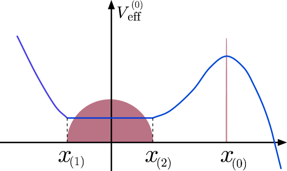
Figure 1: $V_{{\rm eff}}^{(0)}$.

The meaning if this plateau is that the force from the other eigenvalues acting on the eigenvalue we are considering vanishes in this region. This is natural, because inside the sea of eigenvalues, the force should be balanced to zero. Thus if we choose a value of $x$, $x_{*}$, inside the plateau, $V_{{\rm eff}}^{(0)}(x)$ gives the effective potential in the case that we regard its origin as the value at the plateau. In particular, its local maximum $V_{{\rm eff}}^{(0)}(x_{(0)})$ can be regarded as the potential of the instanton that lies at the top of the effective potential $V_{{\rm eff}}^{(0)}$. A simple computation shows that in the double scaling limit we have

$$g=g_{\star}\exp(-\epsilon^{2}t),~{}~{}~{}x=x_{\star}\exp(\epsilon\zeta),~{}~{}~{}N^{2}=\epsilon^{-5}.$$ (2.9)

The height of the potential barrier then becomes

$$N(V_{{\rm eff}}^{(0)}(x_{(0)})-V_{{\rm eff}}^{(0)}(x_{(2)}))=\frac{8\sqrt{3}}{5}t^{\frac{5}{4}},$$ (2.10)

where $t$ is normalized so that the ‘specific heat’ $u$ derived from the free energy $F(t)$ as $u=\ddot{F}$ satisfies the Painlev$\acute{\mbox{e}}$ equation,

$$u^{2}+\frac{1}{6}\ddot{u}=t.$$ (2.11)

Correspondingly, $\zeta$ is normalized so that the disk amplitude obtained by taking the scaling limit of (2.7) becomes

$$\tilde{w}(\zeta)=\left(\zeta-\frac{1}{2}\sqrt{t}\right)\sqrt{\zeta+\sqrt{t}}.$$ (2.12)

Note that (2.10) agrees with the prediction of the Painlev$\acute{\mbox{e}}$ equation, eq:sinstpv) [5]. In §3, we examine how the coefficient as well as the power of $t$ in (1.8) can be determined from the point of view of the matrix model.

2.2 Chemical potential of the instanton

Next we take a closer look at the contribution from the instanton to the free energy. We begin with the partition function $Z_{N}$, which can be written as

$$Z_{N}=\int d\lambda_{1}\cdots d\lambda_{N}G,~{}~{}~{}G=\Delta^{(N)}(\lambda_{1},\cdots,\lambda_{N})^{2}\exp\left(-N\sum_{i=1}^{N}V(\lambda_{i})\right).$$ (2.13)

This can be divided into the sum of the multi-instanton sectors in the large-$N$ limit, where the interactions between the instantons are of ${\cal O}(1/N)$ compared to the leading contributions, as we see below. Thus we write

$$Z_{N}=Z_{N}^{(0\text{-inst})}+Z_{N}^{(1\text{-inst})}+Z_{N}^{(2\text{-inst})}+\cdots,$$ (2.14)

where the $k$-instanton sector is characterized as that in which $k$ eigenvalues are separated from others; that is, they do not lie in the region $x_{(1)}<x<x_{(2)}$.

Let us consider the 1-instanton sector:

$$Z_{N}^{(1\text{-inst})} = N\int_{x<x_{(1)},x_{(2)}<x}dx\int_{x_{(1)}\leq\lambda_{i}\leq x_{(2)}~{}(i\neq N)}\prod_{i=1}^{N-1}d\lambda_{i}G(x,\lambda_{1},\cdots,\lambda_{N-1})$$ (2.15)

$$= N{Z^{\prime}_{N-1}}^{(0\text{-inst})}\int_{x<x_{(1)},x_{(2)}<x}dx\left\langle\det(x-\phi^{\prime})^{2}\right\rangle^{\prime\,(0\text{-inst})}e^{-NV(x)}$$

$$= N{Z^{\prime}_{N-1}}^{(0\text{-inst})}\int_{x<x_{(1)},x_{(2)}<x}dxf(x),$$

where the overall factor $N$ reflects the number of ways of specifying the isolated eigenvalue. Quantities with primes are defined as in (2.5):

$${Z^{\prime}_{N-1}}^{(0\text{-inst})} = \int d\phi^{\prime}e^{-N{\rm tr}V(\phi^{\prime})},$$

$$\left\langle O\right\rangle^{\prime\,(0\text{-inst})} = \frac{1}{{Z^{\prime}_{N-1}}^{(0\text{-inst})}}\int d\phi^{\prime}Oe^{-N{\rm tr}V(\phi^{\prime})}.$$ (2.16)

Here, all eigenvalues of $\phi^{\prime}$ are understood to lie between $x_{(1)}$ and $x_{(2)}$, and

$$f(x)=\left\langle\det(x-\phi^{\prime})^{2}\right\rangle^{\prime\,(0\text{-inst})}e^{-NV(x)}.$$ (2.17)

It is evident that in (2.15) if we change the interval of the integration with respect to $x$ from $\{x<x_{(1)},x_{(2)}<x\}$ to $\{x_{(1)}<x<x_{(2)}\}$, this integral would give the 0-instanton partition function multiplied by $N$. This observation leads us to the relation

$$N{Z^{\prime}_{N-1}}^{(0\text{-inst})}\int_{x_{(1)}<x<x_{(2)}}dxf(x)=NZ_{N}^{(0\text{-inst})}.$$ (2.18)

Thus, we derive the chemical potential of the instanton in terms of the correlator of the matrix model (2.1) as

$$\mu\equiv\frac{Z_{N}^{(1\text{-inst})}}{Z_{N}^{(0\text{-inst})}}=N\frac{\int_{x<x_{(1)},x_{(2)}<x}dx\left\langle\det(x-\phi)^{2}\right\rangle^{(0\text{-inst})}e^{-NV(x)}}{\int_{x_{(1)}<x<x_{(2)}}dx\left\langle\det(x-\phi)^{2}\right\rangle^{(0\text{-inst})}e^{-NV(x)}},$$ (2.19)

where we have used the fact that in the large-$N$ limit (or the double scaling limit) we have

$$f(x)=\left\langle\det(x-\phi)^{2}\right\rangle^{(0\text{-inst})}e^{-NV(x)},$$ (2.20)

as in (2.6).

Similarly, $Z_{N}^{(k\text{-inst})}$ is given as

$$Z_{N}^{(k\text{-inst})} = {}_{N}C_{k}\left({Z^{\prime}_{N-k}}^{(0\text{-inst})}\right)^{k}$$ (2.21)

$$\times \prod_{i=N-k+1}^{N}\left(\int_{x_{i}<x_{(1)},x_{(2)}<x_{i}}dx_{i}\left\langle\det(x_{i}-\phi^{\prime})^{2}\right\rangle^{\prime\,(0\text{-inst})}e^{-NV(x_{i})}\right)$$

$$\times\Delta^{(k)}(x_{N-k+1},\cdots,x_{N})^{2},$$

where the prime indicates quantities of the $(N-k)\times(N-k)$ matrix model. As long as $k\ll N$, the last factor, $\Delta^{(k)}(x_{N-k+1},\cdots,x_{N})^{2}$, can be ignored, because it gives only an ${\cal O}(1/N)$ contribution compared to the leading one. Physically, this corresponds to switching off interactions between instantons (the dilute gas approximation). Then, the above equation becomes

$$Z_{N}^{(k\text{-inst})}={}_{N}C_{k}\left({Z^{\prime}_{N-k}}^{(0\text{-inst})}\right)^{k}\left(\int_{x<x_{(1)},x_{(2)}<x}dxf(x)\right)^{k}.$$ (2.22)

Repeating the same argument, we obtain

$${}_{N}C_{k}\left({Z^{\prime}_{N-k}}^{(0\text{-inst})}\right)^{k}\left(\int_{x_{(1)}<x<x_{(2)}}dxf(x)\right)^{k}={}_{N}C_{k}Z_{N}^{(0\text{-inst})}$$ (2.23)

and

$$\frac{Z_{N}^{(k\text{-inst})}}{Z_{N}^{(0\text{-inst})}}={}_{N}C_{k}\left(\frac{\int_{x<x_{(1)},x_{(2)}<x}dx\left\langle\det(x-\phi)^{2}\right\rangle^{(0\text{-inst})}e^{-NV(x)}}{\int_{x_{(1)}<x<x_{(2)}}dx\left\langle\det(x-\phi)^{2}\right\rangle^{(0\text{-inst})}e^{-NV(x)}}\right)^{k}.$$ (2.24)

This implies that the free energy is in fact given by

$$F=F^{(0\text{-inst})}+\mu.$$ (2.25)

2.3 An instanton as a D-instanton

In this subsection we confirm that the instanton of the matrix model we have considered is indeed the D-instanton in the $c=0$ noncritical string theory.

We first note that in ordinary critical string theory, contributions from a D-brane correspond to adding surfaces with open boundaries. Let us check that this is also the case with our instanton. We rewrite the partition function (2.3) as

$$Z_{N}=\int dx\int d\phi^{\prime}dqd\bar{q}~{}e^{-S^{(1-{\rm inst.)}}-NV(x)},$$ (2.26)

where

$$S^{(1\text{-inst})}=N{\rm tr}V(\phi^{\prime})+\sum_{i=1,2}\bar{q}_{i}(\phi^{\prime}-x)q_{i},$$ (2.27)

and $q_{i}$ is Grassmann odd in the fundamental representation of $U(N-1)$. This implies that if we evaluate the integration over $x$ by using the saddle point value at $x=x_{(0)}$, the interactions over $q$ and $\bar{q}$ provide new contributions from surfaces with open boundaries [16, 17, 18] for the partition function. This can be expressed as

$$\Delta Z_{N}^{(1\text{-inst})}=\raisebox{-35.0pt}{\scalebox{0.4}{\includegraphics{qloop.eps}}}\,\,.$$ (2.28)

From these considerations, we are led to suspect that our instanton is identically the D-instanton.

In order to make a precise comparison with the continuum (Liouville) theory, let us consider a loop amplitude in the instanton background. If we take account of the effect of the instanton, the resolvent can be written

$$\left\langle\frac{1}{N}{\rm tr}\left(\frac{1}{z-\phi}\right)\right\rangle$$ (2.29)

$$= \frac{1}{Z_{N}}\int dx\int d\lambda_{1}\cdots\lambda_{N-1}\frac{1}{N}\left(\frac{1}{z-x}+\sum_{i=1}^{N-1}\frac{1}{z-\lambda_{i}}\right)$$

$$\times\prod_{i=1}^{N-1}(x-\lambda_{i})^{2}\Delta^{(N-1)}(\lambda_{1},\cdots,\lambda_{N-1})^{2}e^{-N\sum_{i=1}^{N-1}V(\lambda_{i})}e^{-NV(x)}$$

$$\sim \frac{Z_{N}^{(0\text{-inst})}}{Z_{N}}\left\langle\frac{1}{N}{\rm tr}\left(\frac{1}{z-\phi}\right)\right\rangle^{(0\text{-inst})}+\frac{Z_{N}^{(1\text{-inst})}}{Z_{N}}\left(\frac{1}{N}\frac{1}{z-x_{(0)}}+\left\langle\frac{1}{N}\sum_{i=1}^{N-1}\frac{1}{z-\lambda_{i}}\right\rangle_{x_{(0)}}\right)$$

$$+\cdots,$$

where we have replaced the integration with respect to $x$ over the interval $x<x_{(1)}$, $x_{(2)}<x$ with the saddle point value at $x=x_{(0)}$, which is valid in the large-$N$ limit, and we have used

$$\left\langle\frac{1}{N}\sum_{i=1}^{N-1}\frac{1}{z-\lambda_{i}}\right\rangle_{x_{(0)}} = \frac{1}{Z_{N}^{(1\text{-inst})}}N\int d\lambda_{1}\cdots\lambda_{N-1}\left(\frac{1}{N}\sum_{i=1}^{N-1}\frac{1}{z-\lambda_{i}}\right)$$

$$\times \prod_{i=1}^{N-1}(x_{(0)}-\lambda_{i})^{2}\Delta^{(N-1)}(\lambda_{1},\cdots,\lambda_{N-1})^{2}e^{-N\sum_{i=1}^{N-1}V(\lambda_{i})}e^{-NV(x_{(0)})}.$$

From (2.29), the resolvent in the 1-instanton background is given by

$$\left\langle\frac{1}{N}{\rm tr}\left(\frac{1}{z-\phi}\right)\right\rangle^{(1\text{-inst})}=\frac{1}{N}\frac{1}{z-x_{(0)}}+\left\langle\frac{1}{N}\sum_{i=1}^{N-1}\frac{1}{z-\lambda_{i}}\right\rangle_{x_{(0)}}.$$ (2.31)

As discussed below [see (2.35)], this gives the resolvent in the 0-instanton sector at leading-order in the large-$N$ limit as

$$\left\langle\frac{1}{N}{\rm tr}\left(\frac{1}{z-\phi}\right)\right\rangle^{(1\text{-inst})}=\left\langle\frac{1}{N}{\rm tr}\left(\frac{1}{z-\phi}\right)\right\rangle^{(0\text{-inst})}+\Delta R^{(1\text{-inst})},$$ (2.32)

$$\Delta R^{(1\text{-inst})}\equiv\frac{1}{N}\frac{1}{z-x_{(0)}}+\left(\left\langle\frac{1}{N}\sum_{i=1}^{N-1}\frac{1}{z-\lambda_{i}}\right\rangle_{x_{(0)}}-\left\langle\frac{1}{N}{\rm tr}\left(\frac{1}{z-\phi}\right)\right\rangle^{(0\text{-inst})}\right).$$ (2.33)

In $\Delta R^{(1\text{-inst})}$, we see that the first term, $1/N\cdot 1/(z-x_{(0)})$, corresponds to the isolated eigenvalue, which is distributed at $x=x_{(0)}$ as a $\delta$-function, and the second term indicates that this eigenvalue causes a distortion of the distribution of the other eigenvalues, as shown by the factor $\prod_{i=1}^{N-1}(x_{(0)}-\lambda_{i})^{2}$ in (LABEL:eqn:backreaction), both of which turn out to be at next-to-leading order. The physical meaning of $\Delta R^{(1\text{-inst})}$ is quite clear. Because it is precisely the contribution from the instanton to the loop amplitude, it can also be computed by using the action (2.27) as surfaces with loops of $q$ and $\bar{q}$. Thus, it is found that $\Delta R^{(1\text{-inst})}$ describes the correction to the loop amplitude from open boundaries:

$$\Delta R^{(1\text{-inst})}=\raisebox{-35.0pt}{\scalebox{0.4}{\includegraphics{loopinst.eps}}},$$ (2.34)

It is not difficult to compute $\Delta R^{(1\text{-inst})}$ explicitly. First, we note that the resolvent is also given by (2.7), even in the instanton background, because it can be derived generically using the Schwinger-Dyson equation. Thus, a different choice of the polynomial $p(z)$ yields a description of a different instanton sector. Because the behavior of $R(z)$ as $z\rightarrow\infty$ fixes the coefficient of the first-order term in $p(z)$, it is a constant term that distinguishes the instanton background. Denoting $p(z)$ in the absence of the instanton by $p_{0}(z)$ , the resolvent in the instanton background is thus given by

$$R(z) = \frac{1}{2}\left(\sqrt{V^{\prime}(z)^{2}+p_{0}(z)+c}+V^{\prime}(z)\right)$$ (2.35)

$$= R_{0}(z)+\frac{c}{4}\frac{1}{\sqrt{V^{\prime}(z)^{2}+p_{0}(z)}}+\cdots,$$

where $R_{0}(z)$ is the resolvent in the absence of the instanton, and $c$ is a certain constant of ${\cal O}(1/N)$ determined below. The above expansion corresponds to the right-hand side of (2.32) term by term. Therefore, $\Delta R^{(1\text{-inst})}(z)$ takes the form

$$\Delta R^{(1\text{-inst})}(z)=\frac{c}{4}\frac{1}{\sqrt{V^{\prime}(z)^{2}+p_{0}(z)}}+\cdots.$$ (2.36)

In order to find the value of $c$ in the case of the single-instanton background, we note that the eigenvalue density $\rho(x)$ is related to $R(z)$ as

$$\rho(x)=-\frac{1}{\pi}{\rm Im}R(x+i0).$$ (2.37)

Using this, we impose the condition that the integration of $\Delta\rho(x)$ corresponding to $\Delta R^{(1\text{-inst})}(z)$ on the small interval around $z=x_{(0)}$ yields $1/N$, which implies that a single eigenvalue is located at $z=x_{(0)}$. This condition amounts to requiring

$$\frac{1}{2\pi i}\oint_{C_{x_{(0)}}}dz\Delta R^{(1\text{-inst})}(z)=\frac{1}{N},$$ (2.38)

where $C_{x_{(0)}}$ is a small circle surrounding $z=x_{(0)}$. This gives

$$c=\frac{8}{N}W^{\prime}_{0}(x_{(0)}),$$ (2.39)

where

$$W_{0}(z)=\frac{1}{2}\sqrt{V^{\prime}(z)^{2}+p_{0}(z)}.$$ (2.40)

Substituting this into (2.36), we find

$$\Delta R^{(1\text{-inst})}(z)=\frac{1}{N}\frac{W^{\prime}_{0}(x_{(0)})}{W_{0}(z)}+\cdots.$$ (2.41)

In the double scaling limit, this quantity remains finite, and the first term gives

$$\frac{3\sqrt{3}}{8}\frac{t^{\frac{1}{4}}}{\tilde{w}(\zeta)}$$ (2.42)

as the instanton correction to the disk amplitude in the absence of the instanton $\tilde{w}(\zeta)$ given in (2.12). It is easy to check that we can obtain exactly the same result obtained from the case of the $\phi^{4}$ potential. This implies that (2.42) is universal. In §4, we see that (2.42) coincides with the results in the Liouville theory, or the loop equations. Therefore, we find that the instanton is identical to the D-instanton in $c=0$ noncritical string theory.

3 Chemical potential of the instanton

We have seen that we can compute various quantities in the D-instanton background by using the matrix model in the previous section. In this section, we show further that the matrix model also makes it possible to obtain a definite value of the chemical potential for the instanton (2.19), namely, the weight of the instanton itself.

We start by computing the numerator in Eq. (2.19). For $x<x_{(1)}$ or $x_{(2)}<x$, we can set $\det(x-\phi)=\exp\left({\rm tr}\,{\rm ln}(x-\phi)\right)$ unambiguously. We hen obtain

$$\left\langle\det(x-\phi)^{2}\right\rangle=\exp\left[2\,\left\langle{\rm tr}\,{\rm ln}(x-\phi)\right\rangle_{\rm c}+\frac{1}{2}\,\left\langle\left(2\,{\rm tr}\,{\rm ln}(x-\phi)\right)^{2}\right\rangle_{\rm c}+\cdots\right]\,,$$ (3.1)

where the subscript “c” denotes the connected Green function. Here, we have omitted tentatively the superscript “0-inst”. We note that

$$\left\langle{\rm tr}\,{\rm ln}(x-\phi)\right\rangle_{\rm c} = \left\langle{\rm tr}\,{\rm ln}(x-\phi)\right\rangle_{\rm disk}+{\cal O}\left(\frac{1}{N}\right)\,,$$

$$\left\langle\left({\rm tr}\,{\rm ln}(x-\phi)\right)^{2}\right\rangle_{\rm c} = \left\langle({\rm tr}\,{\rm ln}(x-\phi))^{2}\right\rangle_{\rm cylinder}+{\cal O}\left(\frac{1}{N^{2}}\right)\,,$$ (3.2)

where the subscripts “disk” and “cylinder” indicate the disk and cylinder amplitudes, respectively. Thus, Eq. (3.1) takes the form

$$\left\langle\det(x-\phi)^{2}\right\rangle e^{-NV(x)}$$ (3.3)

$$= \exp\left[N\,\left(2\,\left\langle\frac{1}{N}\,{\rm tr}\,{\rm ln}(x-\phi)\right\rangle_{\rm disk}-V(x)\right)+2\,\left\langle({\rm tr}\log(x-\phi))^{2}\right\rangle_{\rm cylinder}+{\cal O}\left(\frac{1}{N}\right)\right]$$

$$= \exp\left(-N\,V_{\rm eff}^{(0)}(x)-V_{\rm eff}^{(1)}(x)+{\cal O}\left(\frac{1}{N}\right)\right)\,.$$

The ${\cal O}(N)$-contribution $[-N\,V_{\rm eff}^{(0)}(x)]$ consists of $V_{\rm eff}^{(0)}(x)$ in Eq. (2.8) (as can be checked by differentiation), while the ${\cal O}(N^{0})$-contribution $V_{\rm eff}^{(1)}(x)$ is given by

$$V_{\rm eff}^{(1)}(x) = -2\,\left\langle\left({\rm tr}\,{\rm ln}(x-\phi)\right)^{2}\right\rangle_{\rm cylinder}$$ (3.4)

$$= -2\,{\rm ln}\left(1+\frac{x-\displaystyle{\frac{x_{(1)}+x_{(2)}}{2}}}{\sqrt{(x-x_{(1)})(x-x_{(2)})}}\right)+2\,{\rm ln}2\,.$$

In deriving Eq. (3.4), we have invoked the formula for the cylinder amplitude [15]

$$\left\langle{\rm tr}\left(\frac{1}{x-\phi}\right){\rm tr}\left(\frac{1}{y-\phi}\right)\right\rangle_{\rm cylinder}$$

$$\qquad=\frac{1}{2(x-y)^{2}}\left(\frac{\displaystyle{xy-\frac{1}{2}(x_{(1)}+x_{(2)})(x+y)+x_{(1)}x_{(2)}}}{\sqrt{(x-x_{(1)})(x-x_{(2)})(y-x_{(2)})(y-x_{(1)})}}-1\right)\,.$$ (3.5)

Thus, the cylinder amplitude is given solely by the two endpoints $x_{(1)}$ and $x_{(2)}$ where $x_{(1)}<x_{(2)}$, of the eigenvalue distribution, and it does not depend on any other details of the profile of the potential $V(x)$.

To evaluate the denominator of Eq. (2.19), it is also necessary to evaluate $V_{\rm eff}^{(1)}(x)$ for $x\in[x_{(1)},\,x_{(2)}]$. However, Eq. (3.4) is invalid in this region. For instance, it diverges at $x=x_{(1)}$. This implies that we need to elaborate on the $N$-dependence of the cylinder amplitude. It is necessary to perform the calculation up to the magnitude of $V_{\rm eff}^{(1)}$, that is, the next leading order in $\frac{1}{N}$. If $V_{\rm eff}^{(1)}(x)$ in this region takes the form

$$V_{\rm eff}^{(1)}(x)=-{\rm ln}\,N+[\mbox{finite function of }x]\,,$$ (3.6)

the chemical potential becomes finite, because the $N$ dependence in Eq. (3.6) cancels the overall factor $N$ in Eq. (2.19). The goal of the rest of this section is to demonstrate that this is indeed the case by evaluating the right-hand side of Eq. (2.19) explicitly, using the orthogonal polynomial method. As we see below, $\left<\det(x-\phi)^{2}\right>$ has a compact expression in terms of orthogonal polynomials. The task at hand then reduces to evaluating the explicit forms of orthogonal polynomials in the regions $x\in[x_{(1)},\,x_{(2)}]$, $x<x_{(1)}$ and $x>x_{(2)}$ separately. It turns out that the case $x\in[x_{(1)},\,x_{(2)}]$ requires a more involved analysis, for which we employ a sort of WKB approximation explicitly (where $\hbar=\frac{1}{N}$) in solving the recursion relation for the orthogonal polynomials. By combining these ingredients, we finally obtain the chemical potential $\mu$ and show that $\mu$ is a “universal” quantity, independent of the details of the potential $V(x)$.

3.1 Orthogonal polynomials and $\left<\det(x-\phi)^{2}\right>$

It is known that a set of polynomials $P_{n}(x)=x^{n}+O(x^{n-1})$ ($n\in{\bf Z}_{+}\cup\{0\}$) that obeys the orthogonality condition

$$\int dx\,e^{-NV(x)}\,P_{n}(x)\,P_{m}(x)=h_{n}\,\delta_{nm}\,$$ (3.7)

can be expressed as the expectation value of $\det(x-\phi_{(n)})$ for a system of an $n\times n$ Hermitian matrix $\phi_{(n)}$ with the action $N{\rm tr}\,V(\phi_{(n)})$ [19],

$$P_{n}(x)=\frac{1}{Z_{n}}\,\int d\phi_{(n)}\,e^{-N\,{\rm tr}\,V(\phi_{(n)})}\,\det(x-\phi_{(n)})\,,$$ (3.8)

where $Z_{n}$ is the partition function of that system. Note the coefficient $N$ multiplying the potential $V(\phi_{(n)})$ in the above expression. Equation (3.8) leads us to seek an expression of $\left<\det(x-\phi)^{2}\right>$ in terms of the orthogonal polynomials, for example, something like $\left(P_{N}(x)\right)^{2}$. As a matter of fact, $\left<\det(x-\phi)^{2}\right>$ does have an explicit expression in terms of orthogonal polynomials and the coefficients of the recursion relation satisfied by them. We now demonstrate this point.

Let us first define a new quantity $D_{n}(x)$ as

$$D_{n}(x)\equiv\det_{0\leq i,\,j\leq n-1}(M_{ij}(x))\,,$$ (3.9)

where

$$M_{ij}(x)\equiv\int dx^{\prime}\,e^{-NV(x^{\prime})}\,\sum_{k=0}^{\infty}\frac{1}{\sqrt{h_{i}h_{k}}}P_{i}(x^{\prime})(x-Q)^{2}_{jk}P_{k}(x^{\prime})\,.$$ (3.10)

Thus, $D_{n}(x)$ is the determinant of the $n\times n$ matrix consisting of the first $n\times n$ entries of the matrix $\{M_{ij}(x)\}_{i,\,j\geq 0}$. In the above, $Q_{i,j}$ is defined through the recursion relation for the orthogonal polynomials $\{P_{n}\}_{n\in{\bf Z}_{+}\cup\{0\}}$,

$$xP_{n}(x)=\sum_{m=0}^{\infty}Q_{n,m}P_{m}(x)\,.$$ (3.11)

In particular, for the $n=N$ case we have

$$D_{N}(x)=\left<\det(x-\phi)^{2}\right>\,.$$ (3.12)

It is easy to see that $D_{n}(x)$ satisfies the recursion relation

$$D_{n}(x)=P_{n}^{2}(x)+Q_{n,n-1}\,D_{n-1}(x)\,.$$ (3.13)

It is also straightforward to show that $Q_{n,n+1}=1$, while

$$Q_{n,n-1}=r_{n}\,,$$

$$r_{n}\equiv\frac{h_{n}}{h_{n-1}}\ (n\geq 1)\,,\quad r_{0}\equiv 0\,.$$ (3.14)

Repeated use of the above recursion relation leads to

$$D_{N}(x)=\left(P_{N}(x)\right)^{2}+r_{N}\,\left(P_{N-1}(x)\right)^{2}+\cdots+r_{N}\cdots r_{1}\,\left(P_{0}(x)\right)^{2}\,.$$ (3.15)

This formula is the key equation in the evaluation of $\left<\det(x-\phi)^{2}\right>$, and it enables us to evaluate the chemical potential by using the asymptotic behavior of the orthogonal polynomials. The remaining task is to evaluate the orthogonal polynomials $P_{n}(x)$ and the coefficients $r_{n}$ appearing in the recursion relation up to the next-to-leading order in the $\frac{1}{N}$ expansion. This is done in the following subsection.

3.2 Asymptotic behavior of $P_{n}$

The forms of the orthogonal polynomials in the large-$N$ limit have been determined as follows [20, 21]:

$$P_{n}(x)=\sqrt{\frac{2}{\pi}}\,e^{\frac{N}{2}\,V(x)}\,\frac{1}{\sqrt{(x-x_{(1)})(x-x_{(2)})}}\,\cos\left[N\,\chi_{a}(x)-(N-n)\,\chi_{b}(x)+\chi_{c}(x)\right]\,.$$ (3.16)

The values $\chi_{a},\chi_{b}$ and $\chi_{c}$ are evaluated in Refs. [20], and [21]. Here, let us instead proceed to evaluate them directly from the recursion relation

$$xP_{n}(x)=P_{n+1}(x)+s_{n}P_{n}(x)+r_{n}P_{n-1}\,,$$ (3.17)

where $s_{n}=Q_{n,n}$ in terms of $Q_{n,m}$, in order to determine the behavior of the orthogonal polynomials to next-to-leading order in ${\cal O}\left(\frac{1}{N}\right)$.

At leading order in $\frac{1}{N}$, $P_{n}(x)$ depends on $N$ as $e^{N}$. Hence, it is convenient to consider the ratio

$$k_{n}(x)\equiv\frac{P_{n}(x)}{P_{n-1}(x)}\sim{\cal O}(N^{0})\,,$$ (3.18)

and to expand the recursion relation (3.17) in $\frac{1}{N}$. With respect to $k_{n}(x)$, Eq. (3.17) takes the form

$$x=k_{n+1}(x)+s_{n}+\frac{r_{n}}{k_{n}(x)}\,.$$ (3.19)

We expand $k_{n}(x)$ in $\frac{1}{N}$ as

$$k_{n}(x)=k^{(0)}\left(x,\,\frac{n}{N}\right)+\frac{1}{N}\,k^{(1)}\left(x,\,\frac{n}{N}\right)+{\cal O}\left(\frac{1}{N^{2}}\right)\,.$$ (3.20)

When we take $n$ and $N$ to the infinity and introduce the continuum variable $\xi=\frac{n}{N}$, the leading and next-to-leading orders of the recursion relation (3.19) yield

$$\left(k^{(0)}(x,\,\xi)\right)^{2}+(s(\xi)-x)k^{(0)}(x,\,\xi)+r(\xi)=0\,,$$

$$\left(2k^{(0)}(x,\,\xi)+(s(\xi)-x)\right)k^{(1)}\left(x,\,\xi\right)+k^{(0)}(x,\,\xi)\left(\frac{1}{2}\,\partial_{\xi}s(\xi)+\partial_{\xi}k^{(0)}(x,\,\xi)\right)=0\,,$$

respectively. Here, the continuum limits of $r$ and $s$ are taken as expressed in Eq. (C.8) (see Appendix C). By solving these equations, we find

$$k^{(0)}(x,\,\xi)=\frac{-(s(\xi)-x)\pm\sqrt{(s(\xi)-x)^{2}-4r(\xi)}}{2}\,,$$ (3.22)

where the branch of the square root should be chosen so that $k_{n}(x)\sim x$ as $|x|\rightarrow\infty$ by taking account of the original definition of $k_{n}(x)$. We also find

$$k^{(1)}(x,\,\xi)=-\frac{k^{(0)}(x,\,\xi)\left(\frac{1}{2}\,\partial_{\xi}s(x,\,\xi)+\partial_{\xi}k^{(0)}(x,\,\xi)\right)}{2k^{(0)}(x,\,\xi)+s(\xi)-x}.$$ (3.23)

The expression for $k^{(1)}(x,\,\xi)$ can be further simplified as

$$k^{(1)}(x,\,\xi)=-\frac{1}{2}\,k^{(0)}(x,\,\xi)\partial_{\xi}\,{\rm ln}\,q(x,\,\xi)\,,$$ (3.24)

where

$$q(x,\,\xi) = 2k^{(0)}(x,\,\xi)+s(\xi)-x$$ (3.25)

$$= \pm\sqrt{\left(s(\xi)-x\right)^{2}-4r(\xi)}\,.$$

Now, it is straightforward to write down the expression for $P_{n}(x)$ as a product of the $k_{i}(x)$:

$$P_{n}(x) = \prod_{j=1}^{n}k_{j}(x)=\exp\left[\sum_{j=1}^{n}{\rm ln}\,k_{j}(x)\right]$$ (3.26)

$$= \exp\left[N\int_{0}^{\frac{n}{N}}d\xi\,{\rm ln}\,k^{(0)}(x,\,\xi)+\int_{0}^{\frac{n}{N}}d\xi\,\frac{k^{(1)}(x,\,\xi)}{k^{(0)}(x,\,\xi)}\right.$$

$$\qquad\left.+\frac{1}{2}\left({\rm ln}\,k^{(0)}\left(x,\,\frac{n}{N}\right)-{\rm ln}\,k^{(0)}\left(x,\,0\right)\right)+{\cal O}\left(\frac{1}{N}\right)\right]\,,$$

where we have utilized the following form of the Euler-Maclaurin summation formula to convert the summation into an integral

$$\sum_{j=n_{1}}^{n_{2}}f_{n}=N\int_{\frac{n_{1}}{N}}^{\frac{n_{2}}{N}}d\xi\,f(\xi)+\frac{1}{2}\left(f\left(\frac{n_{2}}{N}\right)-f\left(\frac{n_{1}}{N}\right)\right)+{\cal O}\left(\frac{1}{N}\right)\,.$$ (3.27)

Using the expression (3.24) for $k^{(1)}(x)$ and the facts that $r(0)=0=s(0)$ and $q(x,0)=x=k^{(0)}(x,0)$, we obtain an expression for the asymptotic behavior of the orthogonal polynomials as

$$P_{n}(x) = \exp\left[N\int_{0}^{\frac{n}{N}}d\xi\,{\rm ln}\,k^{(0)}(x,\,\xi)+\frac{1}{2}\,{\rm ln}\,k^{(0)}\left(x,\,\frac{n}{N}\right)-\frac{1}{2}\,{\rm ln}\,q\left(x,\,\frac{n}{N}\right)\right.$$ (3.28)

$$\qquad\left.+{\cal O}\left(\frac{1}{N}\right)\right]$$

$$= \left(\frac{k^{(0)}\left(x,\,\frac{n}{N}\right)}{q\left(x,\,\frac{n}{N}\right)}\right)^{\frac{1}{2}}\,\exp\left[N\int_{0}^{\frac{n}{N}}d\xi\,{\rm ln}\,k^{(0)}(x,\,\xi)\right]\left(1+{\cal O}\left(\frac{1}{N}\right)\right)\,,$$

where $k^{(0)}(x)$ and $q(x,\,\xi)$ are given explicitly by Eqs. (3.22) and (3.25), respectively.

Thus, we have obtained an expression for $P_{n}(x)$, (3.28), for a given (real) value of $x$ by solving this equation in terms of $n$. However, the above expression becomes complex when the argument of the square root in $q(x,\,\xi)$ is negative, i.e., when

$$\left(x-s\left(\frac{n}{N}\right)\right)^{2}-4\,r\left(\frac{n}{N}\right)<0\,.$$ (3.29)

This seems to be a contradiction, because $P_{n}(x)$ should be a real polynomial. To resolve this difficulty, let us consider an actual plot of $P_{n}(x)$. There is a finite region in which it exhibits oscillating behavior with $n$ nodes. This oscillatory region precisely corresponds to the region where the exponent of $P_{n}(x)$ becomes imaginary in the expression (3.28), because $P_{n}(x)$ contains $q(x,\,\xi)$ in its exponent. This suggests that in this oscillatory region, $P_{n}(x)$ in Eq. (3.28) should behave like a trigonometric function.

Now, it is helpful to recall that we have derived the expression (3.28) by starting from a set of linear difference equations. For this derivation, we can draw an analogy with the WKB method in usual quantum mechanics. The important condition here is the same as the continuity condition for the solution at the turning point, where the behavior of the wavefunction changes from decaying behavior in the classically forbidden region to the oscillating behavior in the classically allowed region. Thus, we should multiply the naive expression in Eq. (3.28) by an appropriate phase factor and take its real part. In other words, the phase factor emerging in the analytic continuation of Eq. (3.28) should be combined to make $P_{n}(x)$ a real trigonometric function with an appropriate phase.

In Appendix D, we show that exactly the same argument as for the WKB approximation applies here and, in particular, we should take an extra factor of $2$ into account when Eq. (3.28) is continued into the oscillating region analytically. Noting also that $\left|k^{(0)}(x,\xi)\right|=\sqrt{r(\xi)}$, we obtain the following expression for $P_{n}(x)$ in the oscillating region:

$$P_{n}(x) = 2\left(\frac{\sqrt{r\left(\frac{n}{N}\right)}}{\left|q\left(x,\,\frac{n}{N}\right)\right|}\right)^{\frac{1}{2}}\,\exp\left[N\,{\rm Re}\,\int_{0}^{\frac{n}{N}}d\xi\,{\rm ln}\,k^{(0)}(x,\,\xi)\right]\sin\left(\theta(x)\right)$$ (3.30)

$$\quad\times\left(1+{\cal O}\left(\frac{1}{N}\right)\right)\,.$$

Here $\theta(x)$ represents a phase factor. As there are $n\sim{\cal O}(N)$ nodes located in a finite interval, $\theta(x)$ is expected to vary rapidly, while Eq. (3.30) explicitly shows that the amplitude of the oscillation changes very slowly. For our purposes, it suffices to know the averaged value taken over a small interval around $x$. Taking the average of the square of $P_{n}(x)$ for an interval where $\theta(x)$ should oscillate at least once, we obtain

$$\left(P_{n}(x)\right)^{2}_{\rm averaged} = 2\,\frac{\sqrt{r\left(\frac{n}{N}\right)}}{\left|q\left(x,\,\frac{n}{N}\right)\right|}\,\exp\left[2N\,{\rm Re}\,\int_{0}^{\frac{n}{N}}d\xi\,{\rm ln}\,k^{(0)}(x,\,\xi)\right]$$ (3.31)

$$\quad\times\left(1+{\cal O}\left(\frac{1}{N}\right)\right)\,,$$

which we use hereafter as the asymptotic form of the orthogonal polynomials when $x$ lies in the oscillating region.

3.3 Evaluation of $\left<\det(x-\phi)^{2}\right>$

Now we are ready to evaluate $\left<\det(x-\phi)^{2}\right>$ using the asymptotic behavior of the orthogonal polynomials obtained in the previous section. There is an essential difference between the case in which $x$ is positioned inside the cut, that is, $x_{(1)}<x<x_{(2)}$, and the case in which $x$ is outside the cut.

Let us first consider the case that $x$ is located outside the cut. In (3.15), the ratio of neighboring terms, which we write as $c_{j}(x)$, is

$$c_{j}(x) \equiv \frac{\left(P_{N-j-1}(x)\right)^{2}r_{N-j}}{\left(P_{N-j}(x)\right)^{2}}=\frac{r_{N-j}}{\left(k_{N-j}(x)\right)^{2}}$$ (3.32)

$$= \frac{r\left(\frac{N-j}{N}\right)}{\left(k^{(0)}\left(x,\,\frac{N-j}{N}\right)\right)^{2}}+{\cal O}\left(\frac{1}{N}\right)$$

$$= \left.\frac{-(s(\xi)-x)-\sqrt{(s(\xi)-x)^{2}-4r(\xi)}}{-(s(\xi)-x)+\sqrt{(s(\xi)-x)^{2}-4r(\xi)}}\right|_{\xi=\frac{N-j}{N}}+{\cal O}\left(\frac{1}{N}\right)\,.$$

The quantity $c_{j}(x)$ is of ${\cal O}(N^{0})$ and less than 1. Therefore, the largest contribution to $\left<\det(x-\phi)^{2}\right>$ comes from the first term $P_{N}(x)^{2}$. Note also that the dependence of $c_{j}(x)$ on $j$ is modest [i.e. ${\cal O}(N^{0})$] compared to the number [${\cal O}(N)$] of terms. Hence, when the sum is replaced by a sum of terms with a constant ratio, say $c_{0}(x)$, the correction will be of order $\frac{1}{N}$:

$$\left<\det(x-\phi)^{2}\right> = \left(P_{N}(x)\right)^{2}\sum_{j=0}^{N}\left(c_{0}(x)\right)^{j}\left(1+{\cal O}\left(\frac{1}{N}\right)\right)$$ (3.33)

$$= \left(P_{N}(x)\right)^{2}\,\frac{1}{1-c_{0}(x)}\left(1+{\cal O}\left(\frac{1}{N}\right)\right)\,.$$

The factor $\frac{1}{1-c_{0}(x)}$ turns out to be

$$\frac{1}{1-c_{0}(x)} = \frac{-(s(1)-x)+\sqrt{(s(1)-x)^{2}-4r(1)})}{2\sqrt{(s(1)-x)^{2}-4r(1)}}$$ (3.34)

$$= \frac{k^{(0)}(x,\,1)}{q(x,\,1)}\,.$$

Hence, we obtain

$$\left<\det(x-\phi)^{2}\right>=\left(\frac{k^{(0)}\left(x,\,1\right)}{q\left(x,\,1\right)}\right)^{2}\exp\left[2N\int_{0}^{1}d\xi\,{\rm ln}\,k^{(0)}\left(x,\,\xi\right)\right]\left(1+{\cal O}\left(\frac{1}{N}\right)\right).$$ (3.35)

Next, we evaluate $\left<\det(x-\phi)^{2}\right>$ for the case that $x$ lies inside the cut, that is, in $[x_{(1)},x_{(2)}]$. Note first, as briefly described in the previous subsection, the orthogonal polynomials $P_{n}(x)$ have the following oscillatory behavior: (1) $P_{n}(x)$ oscillates within a finite region in which it has $n$ nodes. The amplitude of each oscillation itself varies slowly, so that we can draw a curve enveloping these oscillations. Outside this oscillatory region, $P_{n}(x)$ behaves as $x^{n}$. (2) This oscillatory region grows as $n$ becomes large. For sufficiently large $n$, this region becomes the region in which $k^{(0)}$ becomes imaginary,

$$\left(x-s\left(\frac{n}{N}\right)\right)^{2}-4r\left(\frac{n}{N}\right)<0.$$ (3.36)

Thus, the main contribution to $D_{N}$ comes from the terms contains $P_{m}(x)$ with $m>n_{0}$, where the integer $n_{0}$ for a given $x$ is defined by

$$\left(x-s\left(\frac{n_{0}(x)}{N}\right)\right)^{2}-4r\left(\frac{n_{0}(x)}{N}\right)=0.$$ (3.37)

We can repeat the argument that leads to (3.33) for this case. We can thereby show that the contribution from $P_{m}(x)$ for $m<n_{0}(x)$ is suppressed exponentially, because the ratio of the neighboring terms is less than 1. Hence, $\left<\det(x-\phi)^{2}\right>$ can be approximated as

$$\left<\det(x-\phi)^{2}\right>=\sum_{i=n_{0}(x)}^{N}\left(P_{i}(x)\right)^{2}\prod_{j=0}^{N-1-i}r_{N-j}\,.$$ (3.38)

From the expression for $\left(P_{i}(x)\right)^{2}$ in (3.31) and an additional calculation presented in Appendix E, we obtain

$$\left<\det(x-\phi)^{2}\right>_{\rm averaged} = 2N\,\pi\,\sqrt{r(1)}\,\rho(x)\,\exp\left[2N\int_{0}^{\xi_{0}(x)}d\xi\,{\rm ln}\,k^{(0)}(\xi)+N\int_{\xi_{0}(x)}^{1}d\xi\,{\rm ln}\,r(\xi)\right]$$ (3.39)

$$\quad\times\left(1+{\cal O}\left(\frac{1}{N}\right)\right)\,,$$

where $\xi_{0}(x)=\frac{n_{0}(x)}{N}$ and $\rho(x)$ is the eigenvalue density (2.37).

We summarize the above result in the form of the effective potential $V_{\rm eff}$ from the relation $e^{-N(V_{\rm eff}(x)-V(x))}=\left<\det(x-\phi)^{2}\right>$.

$$\mbox{\rm Outside the cut:}\qquad V_{\rm eff}(x) = V(x)-2\int^{1}_{0}d\xi{\rm ln}k^{(0)}(\xi)$$

$$-\frac{1}{N}\Big{\{}-\log[(x-s(1))^{2}-4r(1)]$$

$$+2\log\left(x-s(1)+\sqrt{(x-s(1))^{2}-4r(1)}\right)-2\log 2\Big{\}}.$$

$$\mbox{\rm Inside the cut:}\qquad V_{\rm eff}(x) = V(x)-2\int_{0}^{\xi_{0}(x)}d\xi\,{\rm ln}\,k^{(0)}(\xi)-\int_{\xi_{0}(x)}^{1}d\xi\,{\rm ln}\,r(\xi)$$ (3.41)

$$\qquad-\frac{1}{N}\log\left[2N\pi\rho(x)\sqrt{r(1)}\right].$$

Also, if we use $V_{\rm eff}^{(0)}$ in Eq. (2.8), the above expressions can be cast into much simpler forms.

$$\mbox{\rm Outside the cut:}\qquad V_{\rm eff}(x) = V_{\rm eff}^{(0)}(x)-\frac{1}{N}\left\{-2\log\left[\frac{k^{(0)}(x,1)}{q(x,1)}\right]\right\}.$$ (3.42)

$$\mbox{\rm Inside the cut:}\qquad V_{\rm eff}(x) = V_{\rm eff}^{(0)}(x)-\frac{1}{N}\log\left[2N\pi\rho(x)\sqrt{r(1)}\right].$$ (3.43)

3.4 Universality of the chemical potential of the instanton

Now we are ready to take the ratio of the partition functions existing inside and outside the cut. They are given by the integral of $V_{\rm eff}$ above obtained for the respective regions. We evaluate this ratio, the chemical potential of the instanton, near the critical point.

We can evaluate the contribution from outside the cut using the saddle point method. To do this, let us first evaluate the leading contribution to $V_{\rm eff}$, that is the first two terms on the right-hand side of (3.3),

$$V(x)-2\int^{1}_{0}d\xi{\rm ln}k^{(0)}(\xi).$$

Near the critical point, as explained in Appendix C, $r$ and $s$ behave as

$$r = r_{c}-\frac{1}{2}\alpha r_{c}\sqrt{1-\xi+\Delta\kern-1.5ptg},$$ (3.44)

$$s = s_{c}-\frac{1}{2}\alpha\sqrt{r_{c}}\sqrt{1-\xi+\Delta\kern-1.5ptg},$$ (3.45)

where $\Delta\kern-1.5ptg$ represents the deviation from the critical point and $\alpha$ is a certain constant. If we rescale $x$ and $\xi$ to emphasize the region near the critical point as

$$x = s_{c}+2\sqrt{r_{c}}+\sqrt{\Delta\kern-1.5ptg}\zeta,$$ (3.46)

$$\xi = 1-\Delta\kern-1.5ptg\eta,$$ (3.47)

$V_{\rm eff}$ can be expanded in terms of $\Delta\kern-1.5ptg$ as

$$V_{\rm eff}\sim V(x)-\int_{0}^{\Delta\kern-1.5ptg^{-1}}d\eta\Delta\kern-1.5ptg\left(2\ln(\sqrt{r_{c}})+\Delta\kern-1.5ptg^{\frac{1}{4}}\frac{2\sqrt{\zeta\sqrt{r_{c}}+r_{c}\alpha\sqrt{\eta+1}}}{\sqrt{r_{c}}}+{\cal O}(\Delta\kern-1.5ptg^{\frac{1}{2}})\right).$$ (3.48)

We are interested in the universal part of the derivative of $V_{\rm eff}$ rather than $V_{\rm eff}$ itself. In other words, we are interested in the term proportional to $\Delta\kern-1.5ptg^{\frac{5}{4}}$, which can be obtained in the following familiar form after integrating over $\eta$:

$$V^{\prime}_{\rm eff}(\zeta)\sim-\frac{8}{3}\Delta\kern-1.5ptg^{\frac{5}{4}}\frac{\left(\zeta-\frac{1}{2}\sqrt{r_{c}}\alpha\right)\sqrt{\zeta+\sqrt{r_{c}}\alpha}}{r_{c}^{\frac{5}{4}}\alpha^{2}}.$$ (3.49)

Thus, at leading order, the integral $\int dxe^{-V_{\rm eff}}$ can be evaluated at the saddle point, $\zeta=\frac{1}{2}\sqrt{r_{c}}\alpha$. At the next-to-leading order, that is, for the contribution from the cylinder part, we can use the same saddle point as that at leading order. The standard saddle point calculation yields

$$\int_{x<x_{(1)},x_{(2)}<x}dxe^{-NV_{\rm eff}(x)}=\frac{i}{12}\frac{3^{\frac{1}{4}}2^{\frac{1}{4}}\sqrt{\pi}\sqrt{r_{c}}}{\alpha^{\frac{1}{4}}\Delta\kern-1.5ptg^{\frac{5}{8}}\sqrt{N}}e^{-NV_{\rm eff}^{(0)}(x_{0})}.$$ (3.50)

The contribution from inside the cut is simpler to evaluate. Noting that for this case, $V_{\rm eff}^{(0)}(x)$ takes a constant value, say $V_{\rm eff}^{(0)}(x_{(2)})$, and we can replace $r_{N}$ with $r_{c}$, it is straightforward to obtain

$$\int_{x_{(1)}<x<x_{(2)}}dxe^{-NV_{\rm eff}(x)}=\int_{x_{(1)}<x<x_{(2)}}dx2N\pi\rho(x)\sqrt{r_{N}}e^{-NV_{\rm eff}^{(0)}(x)}=2N\pi\sqrt{r_{c}}e^{-NV_{\rm eff}^{(0)}(x_{(2)})}.$$ (3.51)

In passing, we note that we can perform another calculation that leads rather directly to (3.51). This calculation, which we present in Appendix E, does not involve the explicit form of $V_{\rm eff}(x)$.

Taking the ratio of (3.50) and (3.51), we finally obtain the chemical potential of the instanton (2.19) as

$$\mu=\frac{i}{24}\frac{3^{\frac{1}{4}}2^{\frac{1}{4}}}{\alpha^{\frac{1}{4}}\Delta\kern-1.5ptg^{\frac{5}{8}}\sqrt{\pi}\sqrt{N}}e^{-N\left(V_{\rm eff}^{(0)}(x_{(0)})-V_{\rm eff}^{(0)}(x_{(2)})\right)}.$$ (3.52)

To make a connection with the standard analysis, we need to rewrite the chemical potential (3.52) in terms of a quantity that appears in the string equation. The solution of the string equation is the second derivative of the free energy, and it is conventionally normalized so that $\ddot{F}\sim-\sqrt{t}$. With this normalization, the free energy is given by

$$-\frac{4}{15}t^{\frac{5}{2}}.$$ (3.53)

On the other hand, the free energy of the matrix model is obtained as

$$F_{\rm matrix}=N^{2}\int^{1}_{0}(1-\xi)\log(r(\xi))d\xi.$$ (3.54)

Near the critical point, $r$ behaves as (3.44). Expanding $F_{\rm matrix}$ in terms of $\Delta\kern-1.5ptg$ and taking the first non-integer exponent yields the universal part of the free energy as

$$-\frac{2N^{2}\alpha\Delta\kern-1.5ptg^{\frac{5}{2}}}{15}.$$ (3.55)

By comparing (3.53) and (3.55), we can connect $\Delta\kern-1.5ptg$ with $t$ in the string equation as

$$\Delta\kern-1.5ptg=\frac{2^{\frac{2}{5}}t}{\alpha^{\frac{2}{5}}N^{\frac{4}{5}}}.$$ (3.56)

Using this relation and invoking Eq. (2.10), we reach the universal expression for the chemical potential

$$\mu=\frac{Z_{N}^{({1\text{-inst}})}}{Z_{N}^{({0\text{-inst}})}}=\frac{i}{8\cdot 3^{\frac{3}{4}}\sqrt{\pi}t^{\frac{5}{8}}}e^{-\frac{8\sqrt{3}}{5}t^{\frac{5}{4}}}.$$ (3.57)

If $V(x)$ is an even function, the above argument needs two modifications, due to the accidental symmetry of the potential with respect to the exchange of $x$ and $-x$. First, $s$ vanishes identically. However, (3.48), (3.49), (3.50) and (3.52) hold if we replace $\alpha$ with $\frac{\alpha}{2}$ in these equations. Then (3.52) becomes

$$\frac{i}{24}\frac{3^{\frac{1}{4}}2^{\frac{1}{2}}}{\alpha^{\frac{1}{4}}\Delta\kern-1.5ptg^{\frac{5}{8}}\sqrt{\pi}\sqrt{N}}e^{-N\left(V_{\rm eff}^{(0)}(x_{(0)})-V_{\rm eff}^{(0)}(x_{(2)})\right)}.$$ (3.58)

Secondly, there emerge two critical points corresponding to two maximum points of the potential that have exactly the same height. Each critical point contributes the same amount to the free energy, and therefore the value of the free energy is twice that in generic potential cases. Taking this effect into account, (3.53) should be

$$-\frac{8}{15}t^{\frac{5}{2}}.$$ (3.59)

On the other hand, because $s$ does not contribute to the free energy, (3.55) does not change. Thus the relation between $\Delta g$ and $t$ becomes

$$\Delta g=\frac{2^{\frac{4}{5}}t}{\alpha^{\frac{2}{5}}N^{\frac{4}{5}}}.$$ (3.60)

Substituting this relation into (3.58), we reach the same result. Hence, it is concluded that (3.57) is universal. As a concrete example, we present a computation of $\mu$ in the cases of both the $\phi^{3}$ and $\phi^{4}$ potentials in Appendix F.

4 D-instanton effect in loop equations

The Schwinger-Dyson equations for the correlation functions of the “loop variables” ${\rm tr}\,\phi^{n}$ are known as the loop equations, and it is believed that they give a complete description of the system. Their continuum limit is easily taken [22], and the result can be interpreted as a sort of closed string field theory [23, 24, 25]. The loop variables are also useful when we compare the matrix model with the Liouville field theory.

In this section, we consider the question of what properties of the instantons observed in the previous sections can be captured by the continuum loop equations. After some preparation in §4.1, we examine the classical limit ($g_{\rm st}\rightarrow 0$) of the loop equations in §4.2, and we see that in the single-instanton vacuum, the classical solution for the loop amplitude has an ambiguity in the form of an arbitrary constant factor. In §4.3, we show that this constant factor can be determined if we consider the loop equations to all orders. In §4.4, we first show that the single-instanton loop amplitude obtained in this manner indeed is identical to that obtained from the matrix model calculation. We next compute the D-instanton effect on the loop amplitude in the Liouville field theory, and we find that it too reproduces the result of the matrix model. This coincidence confirms that the instanton in the matrix model is identical to the D-instanton in the Liouville field theory.

To this point, we have seen that the loop equations correctly describe the loop amplitude in each vacuum with a fixed number of instantons. However, the continuum loop equations cannot determine the chemical potential of the instanton. In §4.5, we see that the continuum loop equations give a divergent expression and require regularization when we attempt to evaluate the chemical potential.

4.1 Loop equations

In this subsection, we make a few remarks on the loop equations that will be important in the succeeding analysis. If we start with the matrix model with the action

$$S=N\,{\rm tr}\,V(\phi)\,,$$

$$V(x)=\sum_{m=1}^{p}\frac{c_{m}}{m}\,x^{m}\,,$$ (4.1)

the loop equations can be derived from the Schwinger-Dyson equations

$$0=\int d\phi\,\frac{\partial}{\partial\phi^{a}}\left[{\rm tr}\left(t^{a}\phi^{n_{0}}\right)\,W_{n_{1}}\cdots W_{n_{r}}e^{-N\,{\rm tr}\,V(\phi)}\right]\,.$$ (4.2)

Here, $W_{n}$ is the loop variable

$$W_{n}=\frac{1}{N}\,{\rm tr}\,\phi^{n}\,,$$ (4.3)

and $\phi=\phi^{a}t^{a}$ with the $U(N)$ generator $t^{a}$ normalized so that ${\rm tr}(t^{a}t^{b})=\delta^{ab}$. Using

$${\rm tr}(t^{a}A)\,{\rm tr}(t^{a}B)={\rm tr}(AB)$$

$${\rm tr}(t^{a}A\,t^{a}B)={\rm tr}A\,{\rm tr}B\,,$$ (4.4)

we can show that Eq. (4.2) takes the form

$$\sum_{j=0}^{n_{0}-1}\left<W_{j}W_{n_{0}-1-j}W_{n_{1}}\cdots W_{n_{r}}\right>-\sum_{m=1}^{p}c_{m}\left<W_{n_{0}+m-1}W_{n_{1}}\cdots W_{n_{r}}\right>$$

$$\quad+\frac{1}{N^{2}}\sum_{s=1}^{r}n_{s}\left<W_{n_{1}}\cdots W_{n_{s-1}}W_{n_{s}-1+n_{0}}W_{n_{s+1}}\cdots W_{n_{r}}\right>=0\,.$$ (4.5)

We would like to find the form of Eq. (4.5) in the double scaling limit, expressed by

$$g = g_{\star}\,e^{-a^{2}\,\beta\,t}\,,$$

$$x = x_{\star}\,e^{a\,\gamma\,\zeta}\,,$$

$$\frac{1}{N} = a^{\frac{5}{2}}\,\kappa\,g_{s}\,,$$ (4.6)

for $\phi^{3}$-theory in which $V(x)=\frac{1}{2}\,x^{2}-\frac{g}{3}\,x^{3}$, and by

$$g = g_{\star}\,e^{-a^{2}\,\beta\,t}\,,$$

$$x = x_{\star}\,e^{a\,\gamma\,\zeta}\,,$$

$$\frac{1}{N} = a^{\frac{5}{2}}\,\kappa\,g_{s}\,,$$ (4.7)

for $\phi^{4}$-theory in which $V(x)=\frac{1}{2}\,x^{2}-\frac{g}{4}\,x^{4}$. In Eqs. (4.6) and (4.7), $x_{\star}$ and $g_{\star}$ represent the critical values of $x$ and $g$, whose values, as well as those of $\beta$, $\gamma$ and $\kappa$, are given explicitly in Appendices A and B for $\phi^{3}$-theory and $\phi^{4}$-theory, respectively. If we take the continuum loop length $l$ as $l=\gamma na$, $W_{n}$ approaches the continuum loop operator $w(l)$ in the double scaling limit as

$$W_{n}\rightarrow a^{\frac{5}{2}}x_{\star}^{n+1}\gamma Z_{W}^{\frac{1}{2}}\,w(l)\,,$$ (4.8)

where the constant $Z_{W}$ is given by

$$Z_{W}=6\gamma^{3}(g_{\star}x_{\star})^{3}\quad\mbox{for $\phi^{3}$-theory}\,$$ (4.9)

and

$$Z_{W}=\left(\frac{8}{3}\right)^{2}\gamma^{3}\quad\mbox{for $\phi^{4}$-theory}\,.$$ (4.10)

Using this, we can show that the loop equations (4.5) have the following continuum form in the double scaling limit [23]:

$$l\int_{0}^{l}dl^{\prime}\left<w(l^{\prime})\,w(l-l^{\prime})\,w(l_{1})\cdots w(l_{r})\right>+\rho_{s}(l)\left<w(l_{1})\cdots w(l_{r})\right>$$

$$\quad+g_{\rm st}^{2}\,l\sum_{s=1}^{r}l_{s}\left<w(l_{1})\cdots w(l_{s-1})w(l_{s}+l)w(l_{s+1})\cdots w(l_{r})\right>=0\,,$$

$$\rho_{s}(l)\equiv 3\,\delta^{\prime\prime}(l)-\frac{3}{4}\,t\delta(l)\,.$$ (4.11)

We note that $g_{\rm st}$ appearing in Eq. (4.11) differs from $g_{s}$ in the matrix model by the factor

$$g_{\rm st}=\frac{1}{\sqrt{Z_{W}}}\,\frac{\kappa}{\gamma x_{\star}}\,g_{s}\,.$$ (4.12)

Using $Z_{W}$ in Eq. (4.10) and the values for $\beta$, $\gamma$ and $\kappa$ given in Appendices A and B, we find that the conversion factor $\frac{1}{\sqrt{Z_{W}}}\,\frac{\kappa}{\gamma x_{\star}}$ takes the same value in both $\phi^{3}$-theory and $\phi^{4}$-theory,

$$g_{\rm st}=\frac{3}{4\sqrt{2}}\,g_{s}\,.$$ (4.13)

We also remark that we employ such a convention that the same renormalized cosmological constant $t$ and renormalized boundary cosmological constant $\zeta$ can be used in the loop equations and the matrix model. Therefore, we can compare the quantities in the loop equations with those in the matrix model by taking account of the conversion factor (4.13) for the string coupling constants.

To treat the coupled equations (4.11), we introduce canonical pairs $\psi(l)$ and $\psi^{\dagger}(l)$ of closed string fields that satisfy the relations

$$\displaystyle{\left[\psi(l),\,\psi^{\dagger}(l^{\prime})\right]=\delta(l-l^{\prime})\,,}$$

$$\displaystyle{\left[\psi(l),\,\psi(l^{\prime})\right]=0=\left[\psi^{\dagger}(l),\,\psi^{\dagger}(l^{\prime})\right]\,,}$$ (4.14)

and the “vacuum” state $\left|0\right>$ that is annihilated by all $\psi(l)$ i.e., for which we have $\psi(l)\left|0\right>=0$ ($\left<0\right|\psi^{\dagger}(l)=0$). We then define the state $\left|\Psi\right>$ by

$$\left|\Psi\right> = \sum_{r=0}^{\infty}\frac{1}{r!}\int_{0}^{\infty}dl_{1}\,\psi^{\dagger}(l_{1})\cdots\int_{0}^{\infty}dl_{r}\,\psi^{\dagger}(l_{r})\left|0\right>\left<w(l_{1})\cdots w(l_{r})\right>$$ (4.15)

$$= \exp\left[\sum_{r=1}^{\infty}\frac{1}{r!}\int_{0}^{\infty}dl_{1}\,\psi^{\dagger}(l_{1})\cdots\int_{0}^{\infty}dl_{r}\,\psi^{\dagger}(l_{r})\,w^{(r)}\left(l_{1},\cdots,l_{r}\right)\right]\left|0\right>\,,$$

where $w^{(r)}\left(l_{1},\cdots,l_{r}\right)$ represents the connected part of the Green function $\left<w(l_{1})\cdots w(l_{r})\right>$:

$$\left<w(l)\right>=w^{(1)}(l)\,,$$

$$\left<w(l_{1})w(l_{2})\right>=w^{(2)}(l_{1},\,l_{2})+w^{(1)}(l_{1})w^{(1)}(l_{2})\,,$$

$$\cdots\,.$$ (4.17)

Using $\left|\Psi\right>$, the original Green functions can be expressed as

$$\left<w(l_{1})\cdots w(l_{r})\right>=\left<0\right|\psi(l_{1})\cdots\psi(l_{r})\left|\Psi\right>\,,$$ (4.18)

and the continuum loop equations (4.11) can be written in the compact form

$$D(l)\left|\Psi\right>=0\,,$$ (4.19)

where

$$D(l)\equiv lT(l)+\rho_{s}(l)\,,$$

$$T(l)\equiv\int_{0}^{l}dl^{\prime}\,\psi(l^{\prime})\,\psi(l-l^{\prime})+g_{\rm st}^{2}\int_{0}^{\infty}dl^{\prime}\,l^{\prime}\,\psi^{\dagger}(l^{\prime})\,\psi(l+l^{\prime})\,.$$ (4.20)

For subsequent considerations, we remark here that $T(l)$ is isomorphic to the energy-momentum tensor in momentum space if $l$ is regarded as a momentum. To see this, we construct a new variable $\varphi(l)$ from $\psi(l)$ and $\psi^{\dagger}(l)$ as

$$\displaystyle{\varphi(l)=\left\{\begin{array}[]{ll}\displaystyle{\frac{\sqrt{2}}{g_{\rm st}}\,\psi(l)}&(l>0)\\ &\\ \displaystyle{\frac{g_{\rm st}}{\sqrt{2}}\,(-l)\psi^{\dagger}(-l)}&(l<0)\end{array}\right.\,.}$$ (4.24)

This variable satisfies the commutation relation

$${\left[\varphi(l),\,\varphi(l^{\prime})\right]=l\delta(l+l^{\prime})\,.}$$ (4.25)

$T(l)$ can then be rewritten as

$$T(l)=g_{\rm st}^{2}\int_{-\infty}^{\infty}dl^{\prime}\,\frac{1}{2}:\varphi(l^{\prime})\,\varphi(l-l^{\prime}):\,.$$ (4.26)

If we further introduce their “coordinate” representation by

$$\widetilde{\varphi}(\sigma) = \frac{1}{i}\int_{-\infty}^{\infty}\frac{dl}{l}\,e^{il\sigma}\,\varphi(l)\,,$$

$$\widetilde{T}(\sigma) = \int_{-\infty}^{\infty}dl\,e^{il\sigma}\,T(l)\,,$$ (4.27)

$\widetilde{T}(\sigma)$ can be expressed as

$$\widetilde{T}(\sigma)=g_{\rm st}^{2}\,\frac{1}{2}:(\partial_{\sigma}\widetilde{\varphi}(\sigma))^{2}:\,,$$ (4.28)

and the two-point Green function of $\partial_{\sigma}\widetilde{\varphi}(\sigma)$ is given by

$$\left<0\right|\partial_{\sigma}\widetilde{\varphi}(\sigma)\partial_{\sigma^{\prime}}\widetilde{\varphi}(\sigma^{\prime})\left|0\right>=\frac{1}{\left(\sigma-\sigma^{\prime}\right)^{2}}\,.$$ (4.29)

Hence, $\widetilde{T}(\sigma)$ is the energy-momentum tensor of a free massless scalar field $\widetilde{\varphi}(\sigma)$ up to an overall factor of $g_{\rm st}^{2}$.

4.2 Classical approximation of the loop equations

This subsection deals with the classical limit, $g_{\rm st}\rightarrow 0$, of the loop equations. In the perturbative expansion, the amplitude $w^{(1)}(l)$ of one external loop begins with the disk contribution $w^{(1)}_{0}(l)$, which is ${\cal O}((g_{\rm st})^{0})$ in our convention (4.16). Because $w^{(2)}(l_{1},\,l_{2})={\cal O}(g_{\rm st}^{2})$ we have

$$\left<w(l_{1})w(l_{2})\right>=w^{(1)}_{0}(l_{1})w^{(1)}_{0}(l_{2})+{\cal O}\left(g_{\rm st}^{2}\right)\,.$$ (4.30)

Thus, Eq. (4.11) with $r=0$ at ${\cal O}((g_{\rm st})^{0})$ becomes

$$\partial_{\zeta}\left(\widetilde{w}(\zeta)\right)^{2}+{\cal O}((g_{\rm st})^{2})=3\zeta^{2}-\frac{3}{4}\,t\,,$$ (4.31)

where $\widetilde{w}(\zeta)$ is the Laplace transform of $w^{(1)}(l)$. This equation determines $\left(\widetilde{w}(\zeta)\right)^{2}$ up to a constant $\varpi$:

$$\left(\widetilde{w}(\zeta)\right)^{2} = \left(\widetilde{w}_{0}(\zeta)\right)^{2}+\varpi\,,$$

$$\left(\widetilde{w}_{0}(\zeta)\right)^{2} = \left(\zeta-\frac{\sqrt{t}}{2}\right)^{2}\left(\zeta+\sqrt{t}\right)\,.$$ (4.32)

In the classical limit, the loop equations do not place a restriction on $\varpi$.

As we have seen in §2, in the matrix model, $\varpi$ is determined by the number of eigenvalues positioned on the top of the potential. By contrast, in the classical approximation of the loop equations, $\varpi$ is ambiguous. This is in some senses obvious from the beginning. It is clear that $\varpi$ cannot be described in terms of classical solutions of closed string field, because it is not of order $g_{\rm st}^{2}$ but rather $g_{\rm st}$.

4.3 Loop equations to all orders and the nonperturbative effect

Beginning in this subsection, we investigate the possibility of determining the constant $\varpi$ and the chemical potential using the loop equations to all orders,(4.19).

First, we examine the vacuum expectation value (VEV) of an operator ${\cal A}$ in the presence of a fixed number of instantons. This means that we pick up, say, a single-instanton sector out of an infinite number of sectors and consider the VEV of ${\cal A}$ in this sector. In the matrix model, such a quantity can be written as

$$\left<{\cal A}\right>^{({\rm 1\mbox{-}inst})} = \frac{Z_{N-1}^{\prime\quad({\rm 0\mbox{-}inst})}}{Z_{N}}\times N\int_{x\sim x_{(0)}}dx\,\left<{\cal A}(\phi^{\prime},\,x)\,\det(x-\phi^{\prime})^{2}\right>^{\prime\,({\rm 0\mbox{-}inst})}\ e^{-NV(x)}$$

$$\propto N\int_{x\sim x_{(0)}}dx\,\left<{\cal A}(\phi^{\prime},\,x)\,\exp\left[2\,{\rm tr}\,{\rm ln}(x-\phi^{\prime})\right]\right>^{\prime\,({\rm 0\mbox{-}inst})}\ e^{-NV(x)}$$

$$= N\int_{x\sim x_{(0)}}dx\,\ e^{-NV(x)}$$

$$\qquad\times\left<{\cal A}(\phi^{\prime},\,x)\,\exp\left[-2\,\int_{0}^{\infty}dl\,\left(\frac{e^{-xl}}{l}\,{\rm tr}\,e^{l\phi^{\prime}}-\frac{e^{-l}}{l}\,{\rm tr}\,1\right)\right]\right>^{\prime\,({\rm 0\mbox{-}inst})}\,,$$

where $Z_{N-1}^{\prime\quad({\rm 0\mbox{-}inst})}$ and $\left<,\,\right>^{\prime\,({\rm 0\mbox{-}inst})}$ are defined in Eq. (2.16).

Because we instead analyze the loop equations here, we need to construct a state describing the single-instanton vacuum by closely considering the expression (LABEL:eq:vev_matrix_model). Equation (LABEL:eq:vev_matrix_model) expresses the VEV of an operator ${\cal A}$ in the single-instanton vacuum in terms of the VEV in the null instanton vacuum of the operator obtained by making the loop of length $l$ (${\rm tr}\,e^{l\phi^{\prime}}$) condensed with a weight $-\frac{2\,e^{-xl}}{l}$ and integrating with respect to $x$ around $x_{(0)}$. In the continuum limit, the null instanton vacuum state $\left|\Psi\right>_{\rm 0\mbox{-}inst}$ is given by

$$\left|\Psi\right>_{\rm 0\mbox{-}inst}=\exp\left[\sum_{r=1}^{\infty}\frac{1}{r!}\int_{0}^{\infty}dl_{1}\,\psi^{\dagger}(l_{1})\cdots\int_{0}^{\infty}dl_{r}\,\psi^{\dagger}(l_{r})\,\left.w^{(r)}\left(l_{1},\cdots,l_{r}\right)\right|_{\rm pert}\right]\left|0\right>\,,$$ (4.34)

where $\left.w^{(r)}(l_{1},\cdots,\,l_{r})\right|_{\rm pert}$ is $w^{(r)}(l_{1},\cdots,\,l_{r})$ in the null instanton vacuum. The single-instanton vacuum state can be obtained by applying the operator ${\cal V}(\zeta)$ to $\left|\Psi\right>_{\rm 0\mbox{-}inst}$, which condenses the loops with an appropriate weight, and then integrating ${\cal V}(\zeta)\left|\Psi\right>_{\rm 0\mbox{-}inst}$ with respect to $\zeta$ around $\frac{\sqrt{t}}{2}$,corresponding to $x_{(0)}$. The operator ${\cal V}(\zeta)$ is obtained by replacing the operator $\frac{1}{N}\,{\rm tr}\,e^{l\phi^{\prime}}$ in the exponent of Eq. (LABEL:eq:vev_matrix_model) with $\psi(l)$:

$${\cal V}(\zeta)=C_{\rm inst}\exp\left[-Q\int_{0}^{\infty}dl\,\frac{2}{l}\,e^{-\zeta l}\,\psi(l)\right]\,.$$ (4.35)

Here, we have introduced the parameter $Q$, to take account of a possible renormalization of the order $N\sim\frac{1}{g_{\rm st}}$, and the overall normalization $C_{\rm inst}$. Using ${\cal V}(\zeta)$ in Eq. (4.35), we obtain the single-instanton vacuum in the form

$$\left|\Psi\right>_{\rm 1\mbox{-}inst} = \int_{\zeta\sim\frac{\sqrt{t}}{2}}d\zeta\,{\cal V}(\zeta)\left|\Psi\right>_{\rm 0\mbox{-}inst}$$ (4.36)

$$= C_{\rm inst}\int_{\zeta\sim\frac{\sqrt{t}}{2}}d\zeta\,\exp\left[-Q\int_{0}^{\infty}dl\,\frac{2}{l}\,e^{-\zeta l}\,\psi(l)\right]\left|\Psi\right>_{\rm 0\mbox{-}inst}\,.$$

Our investigation to this point has not considered the all-order loop equations (4.19). We explain in the following subsections that $Q$ is identical to the constant ambiguity $\varpi$ in the loop amplitude and that $C_{\rm inst}$ is related to the chemical potential. In the rest of this subsection, we would like to find whether $Q$ and $C_{\rm inst}$ can be determined by analyzing the all-order loop equations.

As we have seen above, the operator ${\cal V}(\zeta)$ in Eq. (4.35) has been proposed to introduce an additional instanton into the system if $\zeta$ is integrated around $\frac{\sqrt{t}}{2}$. From the viewpoint of the matrix model, $\displaystyle{\int_{\zeta\sim\frac{\sqrt{t}}{2}}d\zeta\,{\cal V}(\zeta)}$ plays the role of adding an eigenvalue at the top of the potential. Hence, $\displaystyle{\int_{-\infty}^{\infty}d\zeta\,{\cal V}(\zeta)}$ adds an eigenvalue without specifying its position. We recall that the full vacuum $\left|\Psi\right>$ consists of the vacua of various numbers of instantons:

$$\left|\Psi\right>=\left|\Psi\right>_{\rm 0\mbox{-}inst}+\left|\Psi\right>_{\rm 1\mbox{-}inst}+\left|\Psi\right>_{\rm 2\mbox{-}inst}+\cdots\,.$$ (4.37)

Thus, we should have

$$\left|\Psi\right>^{(N+1)}=\int_{-\infty}^{\infty}d\zeta\,{\cal V}(\zeta)\left|\Psi\right>^{(N)}\,,$$ (4.38)

where $\left|\Psi\right>^{(N)}$ is the vacuum of the system consisting of $N$ eigenvalues. In the large-$N$ limit, this equation requires that if $\left|\Psi\right>$ is a solution of the loop equations (4.19), $\displaystyle{\int_{-\infty}^{\infty}d\zeta\,{\cal V}(\zeta)\left|\Psi\right>}$ must also be a solution of these equations. This will be the case if

$$\left[\widetilde{D}(\zeta),\,{\cal V}(\zeta)\right]\sim\partial_{\zeta}{\cal V}(\zeta)\,$$ (4.39)

holds, where $\widetilde{D}(\zeta)$ is the Laplace transform of $D(l)$ . As remarked in §4.1, the operator part of $\widetilde{D}(\zeta)$ is essentially the energy-momentum tensor $\widetilde{T}(\zeta)$. Thus, the above relation implies that ${\cal V}(\zeta)$ should be a primary field of conformal dimension equal to $1$. The works in Ref. [26] carry out a search for such an operator ${\cal V}(\zeta)$ and find an expression in terms of local operators. We find that the primary operator with conformal dimension 1 that resembles Eq. (4.36) is

$$:\exp\left(-i\sqrt{2}\,\widetilde{\varphi}(\sigma)\right):\,=\,:\exp\left[-\int_{0}^{\infty}dl\,\left(\frac{2}{g_{\rm st}l}\,e^{il\sigma}\,\psi(l)-g_{\rm st}\,e^{-il\sigma}\,\psi^{\dagger}(l)\right)\right]:\,.$$ (4.40)

To bring this into the form of Eq. (4.36), we apply the analytic continuation $\sigma\rightarrow i\zeta$, which yields

$${\cal V}(\zeta)\equiv C_{\rm inst}:\exp\left[-\int_{0}^{\infty}dl\,\left(\frac{2}{g_{\rm st}l}\,e^{-\zeta l}\,\psi(l)-g_{\rm st}\,e^{\zeta l}\,\psi^{\dagger}(l)\right)\right]:\,.$$ (4.41)

We thus find that the single-instanton vacuum $\left|\Psi\right>_{\rm 1\mbox{-}inst}$ is given by

$$\left|\Psi\right>_{\rm 1\mbox{-}inst}=D_{\rm inst}\left|\Psi\right>_{\rm 0\mbox{-}inst},$$

$$D_{\rm inst}=C_{\rm inst}\int_{\zeta\sim\frac{\sqrt{t}}{2}}d\zeta:\exp\left[\int_{0}^{\infty}dl\left(-\frac{2}{g_{\rm st}l}\,e^{-\zeta l}\,\psi(l)+g_{\rm st}\,e^{\zeta l}\,\psi^{\dagger}(l)\right)\right]:\,.$$ (4.42)

The expression (4.42) shows that the all-order loop equations determine $Q$ ($Q=\frac{1}{g_{\rm st}}$) appearing in Eq. (4.36). However, the state $\displaystyle{\int_{-\infty}^{\infty}d\zeta\,{\cal V}(\zeta)\left|\Psi\right>}$ with ${\cal V}(\zeta)$ in Eq. (4.41) is always a solution of the loop equations for any value of $C_{\rm inst}$. Thus, the normalization constant $C_{\rm inst}$ cannot be determined as long as we use only closed string fields.

4.4 Loop amplitude in closed string field theory

Now we know how to express the instanton contributions in the loop equation formalism, at least up to an overall normalization. In this subsection, we examine how they appear in the limit $g_{\rm st}\rightarrow 0$. Then, we compare the results of the loop equation with those of the matrix model and the Liouville theory approaches. In particular, as we discussed in §4.2, they should correspond to the solution of Eq. (4.32) with some $\varpi$. We calculate the value of $\varpi$ using the loop equation and compare it with that obtained in the other approaches.

In order to study the limit $g_{\rm st}\rightarrow 0$, it is convenient to express the state (4.42) using Eq. (4.15) as follows:

$$\left|\Psi\right>_{\rm 1\mbox{-}inst} = C_{\rm inst}\int_{\zeta\sim\frac{\sqrt{t}}{2}}d\zeta\,\exp\left(\int_{0}^{\infty}dl\,g_{\rm st}\,e^{\zeta l}\,\psi^{\dagger}(l)\right)$$ (4.43)

$$\qquad\times\exp\left[\sum_{r=1}^{\infty}\frac{1}{r!}\int_{0}^{\infty}dl_{1}\,\left(\psi^{\dagger}(l_{1})-\frac{2}{g_{\rm st}l_{1}}\,e^{-\zeta l_{1}}\right)\times\cdots\right.$$

$$\qquad\qquad\qquad\quad\left.\times\int_{0}^{\infty}dl_{r}\,\left(\psi^{\dagger}(l_{r})-\frac{2}{g_{\rm st}l_{r}}\,e^{-\zeta l_{r}}\right)\right.$$

$$\qquad\qquad\qquad\qquad\left.\times\left.w^{(r)}(l_{1},\cdots,l_{r})\right|_{\rm pert}\right]\left|0\right>\,.$$

Because $w^{(r)}(l_{1},\,\cdots,l_{r})={\cal O}\left((g_{\rm st})^{2(r-1)}\right)$, we can expand Eq.(4.43) in terms of $g_{\rm st}$. Using this expression, let us calculate $\left<0|\Psi\right>_{\rm 1\mbox{-}inst}$ and $\left<0\right|\psi(l)\left|\Psi\right>_{1\mbox{-}\rm inst}$, which can be compared with the quantities calculated in the matrix model formulation.

The quantity $\left<0|\Psi\right>_{\rm 1\mbox{-}inst}$ should be the continuum version of $\int_{x\sim x_{(0)}}dx\,e^{-V_{\rm eff}(x)}$ in the matrix model, and it can be expressed as $\int_{\zeta\sim\frac{\sqrt{t}}{2}}d\zeta\,e^{-V_{\rm eff}(\zeta)}$ in terms of the continuum effective potential $V_{\rm eff}(\zeta)$. Thus, using Eq. (4.43), we find that $V_{\rm eff}(\zeta)$ should be expanded as

$$-V_{\rm eff}(\zeta) = \int_{0}^{\infty}dl\,\left.w^{(1)}(l)\right|_{\rm pert}\,\left(-\frac{2}{g_{\rm st}l}\,e^{-\zeta l}\right)$$ (4.44)

$$\ +\frac{1}{2}\,\int_{0}^{\infty}dl_{1}\,\frac{2}{g_{\rm st}l_{1}}\,e^{-\zeta l_{1}}\,\int_{0}^{\infty}dl_{2}\,\frac{2}{g_{\rm st}l_{2}}\,e^{-\zeta l_{2}}\,\left.w^{(2)}(l_{1},\,l_{2})\right|_{\rm pert}$$

$$\ +\cdots\,.$$

The leading-order contribution to $w^{(1)}(l)$ is from the disk amplitude $w^{(1)}_{0}(l)$. Thus, the above formula to leading order coincides with the matrix model result in the limit $N\rightarrow\infty$. The leading-order contribution to the second term on the right-hand side is from the cylinder amplitude, $w^{(2)}_{0}(l_{1},\,l_{2})$. Higher-order terms involve the contributions from worldsheets with more boundaries. Therefore, the expansion above corresponds to the expansion Eq. (2.28) in the matrix model.

The quantity $\left<0\right|\psi(l)\left|\Psi\right>_{1\mbox{-}\rm inst}$ should correspond to the loop amplitude in the instanton background $\left.w(l)\right|_{\rm inst}$. It is calculated as

$$\left.w(l)\right|_{\rm inst} = \left<0\right|\psi(l)\left|\Psi\right>_{1\mbox{-}\rm inst}$$ (4.45)

$$= C_{\rm inst}\int_{\zeta\sim\frac{\sqrt{t}}{2}}d\zeta\,e^{-V_{\rm eff}(\zeta)}\,$$

$$\quad\times\biggl{[}g_{\rm st}e^{\zeta\,l}$$

$$\qquad+\sum_{r=1}^{\infty}\frac{1}{(r-1)!}\,\int_{0}^{\infty}dl_{1}\left(-\frac{2}{g_{\rm st}l_{1}}\,e^{-\zeta l_{1}}\right)\cdots\int_{0}^{\infty}dl_{r-1}\left(-\frac{2}{g_{\rm st}l_{r-1}}\,e^{-\zeta l_{r-1}}\right)$$

$$\qquad\qquad\qquad\qquad\qquad\qquad\times\left.w^{(r)}(l_{1},\cdots,l_{r-1},\,l)\right|_{\rm pert}\biggl{]}\,.$$

The first few terms in the $g_{\rm st}$ expansion are given as

$$\left.w(l)\right|_{\rm inst} = C_{\rm inst}\int_{\zeta\sim\frac{\sqrt{t}}{2}}d\zeta\,e^{-V_{\rm eff}(\zeta)}\,$$

$$\times \left(\left.w^{(1)}(l)\right|_{\rm pert}+g_{\rm st}e^{\zeta\,l}+\int_{0}^{\infty}dl_{1}\left(-\frac{2}{g_{\rm st}l_{1}}\,e^{-\zeta l_{1}}\right)\left.w^{(2)}_{0}(l_{1},\,l)\right|_{\rm pert}+\cdots\right).$$

In the limit $g_{\rm st}\rightarrow 0$, we can use the saddle point approximation to evaluate the integration over $\zeta$. The saddle point $\zeta=\sqrt{t}/2$ can be identified with $x_{(0)}$ in the matrix model. Thus, by Laplace transforming the above expression, it is easy to see that the three terms in it coincide with the matrix model results Eqs. (2.32) and (2.33).

From the analysis to this point, it is obvious that what we have been doing here is exactly the continuum version of what we did in §2. To be more concrete, Eq. (4.38) should be considered as the continuum version of the manipulation used to isolate the contribution of one eigenvalue by introducing $q_{i}$ and $\bar{q}_{i}$. The value $\zeta$ in Eq. (4.38) corresponds to the eigenvalue $x$ in the continuum limit.

The cylinder amplitude $w^{(2)}_{0}(l_{1},\,l_{2})$ can be obtained by solving Eq. (4.11). It is given as

$$\widetilde{w}^{(2)}_{0}(\zeta_{1},\,\zeta_{2})=-g_{\rm st}^{2}\,\partial_{\zeta_{1}}\partial_{\zeta_{2}}\,{\rm ln}\left(\sqrt{\zeta_{1}+\sqrt{t}}+\sqrt{\zeta_{2}+\sqrt{t}}\right)\,$$ (4.47)

in the Laplace transformed form. Thus $\widetilde{w}|_{\rm inst}(\zeta)=\int_{0}^{\infty}dle^{-\zeta l}w|_{\rm inst}(l)$ is obtained as

$$\widetilde{w}_{0}(\zeta)+g_{\rm st}\left(\frac{1}{\zeta-\frac{\sqrt{t}}{2}}-2\,\partial_{\zeta}{\rm ln}\,\left(\sqrt{\zeta+\sqrt{t}}+\sqrt{\frac{3}{2}}\,t^{\frac{1}{4}}\right)\right)+{\cal O}((g_{\rm st})^{2})$$

$$\quad=\widetilde{w}_{0}(\zeta)+\frac{1}{2}\,\frac{g_{\rm st}\sqrt{6}\,t^{\frac{1}{4}}}{\widetilde{w}_{0}(\zeta)}+{\cal O}((g_{\rm st})^{2})\,.$$ (4.48)

By comparing this with the expansion of $\widetilde{w}(\zeta)$ in $\varpi$ given by Eq. (4.32),

$$\widetilde{w}(\zeta)=\widetilde{w}_{0}(\zeta)+\frac{1}{2}\,\frac{\varpi}{\widetilde{w}_{0}(\zeta)}+{\cal O}((g_{\rm st})^{2})\,,$$ (4.49)

we find that

$$\left.\varpi\right|_{\rm loop\ equation}=g_{\rm st}\sqrt{6}\,t^{\frac{1}{4}}\,.$$ (4.50)

Taking the factor in Eq. (4.13) into account, this value of $\varpi$ is found to coincide with the matrix model result (2.42):

$$\left.\varpi\right|_{\rm matrix}=g_{s}\frac{3\sqrt{3}}{4}\,t^{\frac{1}{4}}\,.$$ (4.51)

This value of $\varpi$ is consistent with the result of the Liouville theory. In the Liouville theory [27], the instanton we have been studying corresponds to the D-instanton. The amplitudes in the presence of such a D-brane can be calculated by using the open string theory. In particular, $w(l)|_{\rm inst}$ can be evaluated as an expansion with respect to the string coupling constant. The first correction to the disk amplitude is given by the cylinder amplitude with one boundary on the D-brane. Thus $\varpi$ can be obtained by calculating such a cylinder amplitude. This is exactly what we have done above.

In the Liouville theory [27], the D-instanton corresponds to the ZZ-brane boundary state $\left|B_{(m,\,n)}\right>_{\rm ZZ}$ with $(m,\,n)=(1,\,1)$. The loop $w(l)$ that we have been discussing corresponds to the FZZT boundary state $\left|B_{s}\right>_{\rm FZZT}$. The normalization of $\left|B_{(m,\,n)}\right>_{\rm ZZ}$ and $\left|B_{s}\right>_{\rm FZZT}$ can be fixed through a modular bootstrap or, in other words, the open-closed duality [8]. Therefore, we need to calculate the cylinder amplitude with one boundary on the ZZ-brane and the other on the FZZT-brane. This can be calculated in a manner similar to that employed in Ref.[11], but here we proceed differently, as we now demonstrate. It is known that the properly normalized boundary states $\left|B_{(m,\,n)}\right>_{\rm ZZ}$ and $\left|B_{s}\right>_{\rm FZZT}$ satisfy the following relation [11, 28, 29] :

$$\left|B_{(m,\,n)}\right>_{\rm ZZ}=\left|B_{s=i\left(\frac{m}{b}+nb\right)}\right>_{\rm FZZT}-\left|B_{s=i\left(\frac{m}{b}-nb\right)}\right>_{\rm FZZT}\,.$$ (4.52)

We have $b=\sqrt{\frac{2}{3}}$ for the $c=0$ case, and $s$ is related to the boundary cosmological constant $\mu_{B}$ and the bulk cosmological constant $\mu$ in the Liouville theory as

$$\cosh(\pi bs)=\frac{\mu_{B}}{\sqrt{\mu}}\,\left(\sin(\pi b^{2})\right)^{\frac{1}{2}}\,.$$ (4.53)

The relation (4.52) can be used to calculate the cylinder amplitude in question from $w^{(2)}_{0}(l_{1},\,l_{2})$ obtained using the loop equation. Thus, we can check if our results are consistent with those obtained from the Liouville approach.

The value of $\mu_{B}$, or equivalently $s$, is obviously related to the variable $\zeta$ we have been using. Because $b=\sqrt{\frac{2}{3}}$, $s=i\left(\frac{1}{b}\pm b\right)$ gives $\cosh(\pi bs)=\frac{1}{2}$. On the other hand, the Laplace transformation of the disk amplitude $\widetilde{w}_{0}$ is proportional to $\cosh(\pi s/b)$. Thus we see that $\widetilde{w}_{0}$ vanishes if $s=i\left(\frac{1}{b}\pm b\right)$. Therefore $s=i\left(\frac{1}{b}\pm b\right)$ should correspond to $\zeta=\frac{\sqrt{t}}{2}$. A careful analysis shows that $s=i\left(\frac{1}{b}+b\right)$ corresponds to $\zeta=\frac{\sqrt{t}}{2}$ on the second Riemann sheet, while $s=i\left(\frac{1}{b}-b\right)$ corresponds to that on the first Riemann sheet.

Now we calculate the cylinder amplitude. The FZZT-brane boundary state can be naturally identified with the boundary formed by $-{\rm tr}\ln(z-\phi)$ in the double-scaled matrix model including the normalization. Therefore, the ${\cal O}(g_{\rm st})$ term in $\widetilde{w}(\zeta)$ should be

$$\int_{0}^{\infty}dl\,e^{-\zeta l}\left[\int_{0}^{\infty}\frac{dl^{\prime}}{l^{\prime}}\,e^{-\zeta^{\prime}l^{\prime}}\frac{w^{(2)}_{0}(l,\,l^{\prime})}{g_{\rm st}}\right]_{\zeta^{\prime}=\frac{\sqrt{t}}{2}\ {\rm on\ the\ first\ Riemann\ sheet}}^{\zeta^{\prime}=\frac{\sqrt{t}}{2}\ {\rm on\ the\ second\ Riemann\ sheet}}\,.$$ (4.54)

Substituting the cylinder amplitude given by Eq. (4.47) into Eq. (4.54), we obtain

$$\left[\frac{g_{\rm st}}{2}\,\frac{\frac{1}{\sqrt{\zeta+\sqrt{t}}}}{\sqrt{\zeta+\sqrt{t}}+\sqrt{\zeta^{\prime}+\sqrt{t}}}\right]_{\zeta^{\prime}=\frac{\sqrt{t}}{2}\ {\rm on\ the\ first\ Riemann\ sheet}}^{\zeta^{\prime}=\frac{\sqrt{t}}{2}\ {\rm on\ the\ second\ Riemann\ sheet}}$$

$$\quad=\frac{g_{\rm st}}{2}\,\frac{1}{\sqrt{\zeta+\sqrt{t}}}\left(\frac{1}{\sqrt{\zeta+\sqrt{t}}-\sqrt{\frac{3}{2}\,\sqrt{t}}}-\frac{1}{\sqrt{\zeta+\sqrt{t}}+\sqrt{\frac{3}{2}\,\sqrt{t}}}\right)$$

$$\quad=\frac{1}{2}\,\frac{g_{\rm st}\sqrt{6}\,t^{\frac{1}{4}}}{\widetilde{w}_{0}(\zeta)}\,.$$ (4.55)

This shows that $\varpi=g_{\rm st}\sqrt{6}\,t^{\frac{1}{4}}$, as anticipated.

The relation in Eq. (4.52) can be seen more directly from the matrix model point of view. Specifically, as we have seen in Eq. (LABEL:eq:vev_matrix_model), adding a single boundary corresponding to the ZZ-brane amounts to inserting $2\,{\rm Re}\,{\rm tr}\ln(z-\phi)$ evaluated at $z=x_{(0)}$ from the matrix model point of view:

$$\left|B_{(1,\,1)}\right>_{\rm ZZ}\longleftrightarrow\left.2\,{\rm Re}\,{\rm tr}\ln(z-\phi)\right|_{z=x_{(0)}}.$$ (4.56)

On the other hand, as we noted above, the FZZT brane corresponds to the integral of the resolvent from the first sheet to the second sheet:

$$\left|B_{s=i\left(\frac{1}{b}+b\right)}\right>_{\rm FZZT}-\left|B_{s=i\left(\frac{1}{b}-b\right)}\right>_{\rm FZZT} \longleftrightarrow -\int_{z=x_{(0)}\ {\rm on\ the\ first\ sheet}}^{z=x_{(0)}\ {\rm on\ the\ second\ sheet}}dz\,{\rm tr}\frac{1}{z-\phi}$$ (4.57)

$$= \left.2\,{\rm Re}\,{\rm tr}\ln(z-\phi)\right|_{z=x_{(0)}}.$$

Because the relation (4.52) was obtained by using the open-closed duality, Eqs. (4.56) and (4.57) suggest that the information concerning the open-closed duality is somehow incorporated in the matrix model.

4.5 Ambiguity in the normalization of single-instanton vacuum state

As we have seen in §4.3, we cannot determine the constant $C_{\rm inst}$ using even the all-order loop equation. For this reason, we cannot determine the chemical potential $\mu$ using this approach. However, as we have shown in §3, $\mu$ can be determined as a universal quantity in the matrix model approach. Therefore, if in the loop equation approach we can mimic as closely as possible the procedure applied in the case of matrix model, we should be able to calculate $\mu$. As we argued in the previous subsection, Eq. (4.38) can be considered the continuum version of the manipulation used to pick up the contribution of one eigenvalue in the matrix model. Hence, we can use this fact as a guide to obtain the continuum version of the calculation of the chemical potential. Although $N$ is $\infty$ in the double scaling limit, here we consider $N$ to be large but finite and take the limit $N\rightarrow\infty$ later. Dividing the integration region into two parts as

$$\left|\Psi\right>^{(N)}=\left(\int_{-\sqrt{t}}^{\infty}d\zeta\,{\cal V}(\zeta)+\int_{-\infty}^{-\sqrt{t}}d\zeta\,{\cal V}(\zeta)\right)\left|\Psi\right>^{(N-1)}\,$$ (4.58)

in Eq. (4.38) (here we have replaced $N$ by $N-1$ for consistency with the matrix model formulation), we can regard the second term on the right-hand side as corresponding to the zero-instanton sector and the first term to the single-instanton sector. In this formulation, $\mu$ can be derived from the ratio of the first term to the second term, and it does not depend on the overall normalization of the operator ${\cal V}$. Let us examine whether we can calculate $\mu$ in this formulation.

In order to calculate $\mu$, we should evaluate $\left<0|\Psi\right>^{(N)}$, which can be expressed as $\int_{-\infty}^{\infty}d\zeta\,e^{-V_{\rm eff}(\zeta)}$. It is very easy to obtain identities similar to Eqs. (4.43) and (4.44) in this case. Because $\zeta>-\sqrt{t}$ corresponds to the single-instanton sector and $-\sqrt{t}>\zeta$ does to the zero-instanton sector, we calculate $V_{\rm eff}(\zeta)$ separately for these two cases.

For $\zeta>-\sqrt{t}$, we can use Eq. (4.44) without any change. In the limit $g_{\rm st}\rightarrow 0$, the leading contribution is from the disk amplitude, and it reproduces the matrix model result in the $N\rightarrow\infty$ limit, up to an additive constant. The cylinder contribution to $-V_{\rm eff}(\zeta)$ is obtained as

$$-2{\rm ln}\left(2\sqrt{\zeta+\sqrt{t}}\right).$$ (4.59)

We expect that the cylinder contribution, which corresponds to the one-loop amplitude for an open string, should contribute to the chemical potential $\mu$.

For $-\sqrt{t}>\zeta$, in evaluating $\left<0|\Psi\right>^{(N)}$, we should fix the value of the loop amplitudes on the cut in the complex $\zeta$ plane. For our purposes, here we should mimic the manner in which we dealt with such an ambiguity in the matrix model. Doing this, we obtain

$$-V_{\rm eff}(\zeta) = \mbox{Re}_{\zeta}\int_{0}^{\infty}dl\,\left.w^{(1)}_{0}(l)\right|_{\rm pert}\,\left(-\frac{2}{g_{\rm st}l}\,e^{-\zeta l}\right)$$ (4.60)

$$\ +\frac{1}{2}\,\mbox{Re}_{\zeta_{1}}\int_{0}^{\infty}dl_{1}\,\frac{2}{g_{\rm st}l_{1}}\,e^{-\zeta_{1}l_{1}}\,\mbox{Re}_{\zeta_{2}}\int_{0}^{\infty}dl_{2}\,\frac{2}{g_{\rm st}l_{2}}\,e^{-\zeta_{1}l_{2}}\,\left.w^{(2)}_{0}(l_{1},\,l_{2})\right|_{\zeta_{1}=\zeta_{2}=\zeta}$$

$$\ +\cdots\,.$$

Here, $\mbox{Re}_{\zeta}$ denotes the operation of taking the real part as a function of $\zeta$. What is relevant for us is the difference $V_{\rm eff}(\frac{\sqrt{t}}{2})-V_{\rm eff}(-\sqrt{t})$ and that the leading-order contribution precisely reproduces the matrix model result. The second term can be evaluated as

$$-\frac{1}{2} \left[{\rm ln}\left(\sqrt{\zeta_{1}+\sqrt{t}}+\sqrt{\zeta_{2}+\sqrt{t}}\right)+{\rm ln}\left(\sqrt{\zeta_{1}+\sqrt{t}}-\sqrt{\zeta_{2}+\sqrt{t}}\right)\right.$$ (4.61)

$$\left.\left.+{\rm ln}\left(-\sqrt{\zeta_{1}+\sqrt{t}}+\sqrt{\zeta_{2}+\sqrt{t}}\right)+{\rm ln}\left(-\sqrt{\zeta_{1}+\sqrt{t}}-\sqrt{\zeta_{2}+\sqrt{t}}\right)\right]\right|_{\zeta_{1}=\zeta_{2}=\zeta}$$

$$\hskip 28.45274pt=-{\rm ln}\left(\zeta_{1}-\zeta_{2}\right)|_{\zeta_{1}=\zeta_{2}=\zeta},$$

which is divergent. The cylinder contribution is, in a sense, continuous at $\zeta=-\sqrt{t}$, because Eq. (4.59) is also divergent when $\zeta\rightarrow-\sqrt{t}$. In any case, because of this divergence, we cannot reproduce the value of the chemical potential $\mu$ in this approach.

If we proceed ignoring this divergence, we obtain the chemical potential as

$$\mu\sim t^{-\frac{1}{2}-\frac{1}{8}}\times N\times\infty^{-1},$$ (4.62)

where the factor $t^{-\frac{1}{2}}$ comes from the cylinder contribution in Eq. (4.59), $t^{-\frac{1}{8}}$ from the Gaussian integration around the saddle point, and $N$ from the combinatorial factor. Therefore, the loop equation approach reproduces the essential part of $\mu$, i.e. $t^{-\frac{5}{8}}$, but it fails to reproduce the precise numerical factor. What we have seen in this subsection is the continuum version of what we observed in the first part of §3. In the matrix model, the divergence is somehow regularized in conjunction with $N$, and we obtain a finite value for $\mu$. In order to calculate $\mu$ in the continuum approach, we might need some renormalization procedure.

Below, we summarize the results obtained for the nonperturbative properties of a noncritical string via the loop equations, or equivalently, the closed string field theory:

(1)

In the classical approximation ($g_{s}\rightarrow 0$) of the loop equations, in a background of D-instantons, we can obtain information regarding the D-instantons through the parameter $Q$ in the instanton creation operator (4.36), which is related to the constant $\varpi$ in the loop amplitude (4.32). However, the value of $Q$ cannot be determined within this approximation.

(2)

The treatment to all orders of the loop equations determines $Q$.

(3)

The chemical potential of the instanton cannot be determined using the loop equation approach.

It may be useful to compare these three results with the results concerning D-branes obtained in critical string theory:

$(1)$

The boundary state for the D-brane is constructed in the closed string theory. The normalization of the boundary state cannot be fixed if only closed strings are considered.

$(2)$

The normalization of the boundary state of the D-brane is determined through comparison with the one-loop amplitude of the open string.

$(3)$

In order to determine the probability of the creation or annihilation of D-branes, which is the same as the chemical potential $\mu$, we need knowledge concerning the nonperturbative dynamics of an open string [10, 12, 13].

Although we do not know the critical string version of what we have done for noncritical string theory using the loop equation approach, we can see that there is a similarity between the situation for critical string theory and that for noncritical string theory.

5 Conclusion

One possible non-perturbative formulation of string theory is that which uses closed string field theory or loop equations. The situation would be simple if string theory could be formulated non-perturbatively using only closed strings. However, what is implied by the facts we have just determined is that a formulation based on only closed strings may not be able to incorporate all of the non-perturbative effects. For example, to calculate the chemical potential for the instanton, we need to know the cut-off dependence of the cylinder contribution. As we have seen, this dependence is well-defined in the matrix model, but not in the loop equations formulated in continuum variables.

Using the loop equations in the classical limit, that is, the large-$N$ limit, one can determine the loop amplitudes in an instanton background, up to a constant factor, which is denoted by $Q$ in §4. Treating the loop equations to all orders, one can further determine this factor. In terms of the D-brane of critical string theory, these two procedures, respectively, correspond to determining the boundary state up to the normalization from the boundary condition and determining the normalization of the boundary state using the one-loop calculation of the open string in the dual channel. Thus, the calculation to all orders of the loop equations is powerful enough to determine the factor that corresponds to the normalization of the boundary state, without the need for the calculation in the dual channel. Despite this fact, however, it cannot determine the chemical potential for an instanton. This corresponds to, in critical string theory, determining the weight of the annihilation and creation of D-branes from the dynamics of the tachyon. We have shown that the matrix model does determine the chemical potential universally. Thus, at least for noncritical string theory, the closed string does not describe the nonperturbative effects completely and it seems that the description offered by the matrix model is more fundamental. If this is also the case for critical string theory, it strongly suggests that the non-perturbative formulation of string theory must contain degrees of freedom corresponding to open strings or matrices.

Because the chemical potential of the D-instanton is a universal quantity, it is conceivable that there exists some continuum approach to calculate it. Open string field theories for noncritical strings have been constructed in Refs. [30]-[33]. It is an intriguing problem to calculate the value of the chemical potential using such theories.

The calculation of the chemical potential employed in this paper is also applicable to other matrix models. The universality of the chemical potential should be checked in the case of other noncritical strings using the two-matrix model, for example. Another interesting matrix model is the two-cut model, which corresponds to super Liouville theory [34]. These problems are left for future studies.

In this paper, we have been attempting to determine the fundamental degrees of freedom in the nonperturbative formulation of string theory. It is suggested that we should incorporate matrix, or at least something that has endpoints, such as an open string. So far our investigation has been limited to the noncritical string theory case. However, it is conceivable that a similar situation exists for critical string theory. Should this issue be settled, it would be a great leap toward answering the ultimate question, What is string theory?

Acknowledgements

The authors would like to thank M. Fukuma, T. Matsuo, S. Matsuura, Y. Sato, S. Sugimoto, F. Sugino, S. Yahikozawa and T. Yoneya for fruitful discussions. This work is supported in part by Grants-in-Aid for Scientific Research (13135101,13135213,13135223, 13135224, 13640308, 15740173) and the Grant-in-Aid for the 21st Century COE “Center for Diversity and Universality in Physics” from the Ministry of Education, Culture, Sports, Science and Technology (MEXT) of Japan. The work of T.K. is supported in part by a Special Postdoctoral Researchers Program.

Appendix A: $\phi^{3}$-theory

In this appendix, we consider one Hermitian matrix model with the partition function

$$Z_{N}=\int d\phi\,\exp\left(-N\,{\rm tr}\,V(\phi)\right)\,,$$

$$V(x)=\frac{1}{2}\,x^{2}-\frac{g}{3}\,x^{3}\,,$$ (A.1)

to explain the convention used in the text. The critical value of the coupling constant in this theory is

$$g_{\star}=\frac{1}{2\cdot 3^{\frac{3}{4}}}\,.$$ (A.2)

We define the square root part of the resolvent $R(z)$ in the null instanton sector by

$$\left(\widetilde{W}_{0}(z)\right)^{2}\equiv\frac{1}{4}\left(\left(V^{\prime}(z)\right)^{2}+f_{0}(z)\right)\,,$$ (A.3)

where $f_{0}(z)$ is a polynomial of degree $1$. For $g<g_{\star}$, $\left(W_{0}(x)\right)^{2}$ has three zeros related as $x_{(1)}<x_{(2)}<x_{(0)}$. The quantity $\left(W_{0}(x)\right)^{2}$ is negative on the interval $(x_{(1)},\,x_{(2)})$, where the eigenvalues are distributed continuously in the large-$N$ limit. At $x_{(0)}$, the first derivative of $\left(W_{0}(x)\right)^{2}$ vanishes . For $g\rightarrow g_{\star}$, $x_{(2)}$ and $x_{(0)}$ coincide at

$$x_{\star}=\frac{3+\sqrt{3}}{6}\,\frac{1}{g_{\star}}\,,$$ (A.4)

while $x_{(1)}$ approaches

$$x_{(1)}(g_{\star})=-\frac{\sqrt{3}-1}{2}\,\frac{1}{g_{\star}}\,.$$ (A.5)

We would like to determine (some ratios of) the constants $\beta$, $\gamma$ and $\kappa$ in the double scaling limit (4.6), so that the string equation and the sphere contribution to the free energy take the forms

$$t=\left(u(t)\right)^{2}-\frac{g_{s}^{2}}{6}\,\partial_{t}^{2}u(t)\,,$$

$$\left.F(t)\right|_{g_{s}\rightarrow 0}=-\frac{1}{g_{s}^{2}}\,\frac{4}{15}\,t^{\frac{5}{2}}\,.$$ (A.6)

After integrating over the angular variables of $\phi$, $Z_{0}$ can be written

$$Z_{0} = \prod_{j=1}^{N}\int d\mu(x_{j})\,\left(\Delta(\{x_{j}\}_{j=1,\,\cdots,\,N})\right)^{2}\,,$$

$$d\mu(x) \equiv dx\,e^{-N\,V(x)}\,,$$ (A.7)

where $\Delta(\{x_{j}\}_{j=1,\,\cdots,\,N})$ is the Vandermonde determinant,

$$\Delta(\{x_{j}\}_{j=1,\,\cdots,\,N})=\prod_{i>j}(x_{i}-x_{j})\,.$$ (A.8)

From the normalization of $P_{n}(x)$, it can be written as

$$\Delta(\{x_{j}\}_{j=1,\,\cdots,\,N})=\det_{1\leq i,\,j\leq N}P_{i-1}(x_{j})\,.$$ (A.9)

By using this and the orthogonality of $\left\{P_{n}\right\}_{n\in{\bf Z}_{+}\cup\{0\}}$, $Z_{0}$ becomes

$$Z_{0} = N!\prod_{n=1}^{N}h_{n-1}$$ (A.10)

$$= N!\prod_{n=1}^{N-1}r_{n}^{N-n}$$

$$= \exp\left({\rm ln}\,N!+\sum_{n=1}^{N-1}(N-n)\,{\rm ln}\,r_{n}\right)\,,$$

where $r_{n}$ is defined by

$$r_{n}\equiv\frac{h_{n}}{h_{n-1}}\quad(n\in{\bf Z}_{+})\,.$$ (A.11)

By subtracting ${\rm ln}\,N!$, the free energy $F={\rm ln}\,Z_{0}$ takes the form

$$F=\sum_{n=1}^{N-1}(N-n)\,{\rm ln}\,r_{n}\,.$$ (A.12)

In order to compute $F$, we need to know $\{r_{n}\}$. From the equations

$$nh_{n+1} = \int d\mu(x)\,\frac{dP_{n}(x)}{dx}\,P_{n-1}(x)\,,$$

$$0 = \int dx\,\frac{d}{dx}\left(e^{-N\,V(x)}\left(P_{n}(x)\right)^{2}\right)\,,$$ (A.13)

the recursion relations for $\{r_{n}\}$ and $\{s_{n}\}$ can be derived:

$$r_{n}\left(1-g\left(s_{n}+s_{n+1}\right)\right)=\frac{n}{N}\,,$$

$$s_{n}^{2}-\frac{1}{g}\,s_{n}+r_{n}+r_{n+1}=0\,.$$ (A.14)

The existence of the weak coupling limit $g\rightarrow 0$ selects one of the solutions of the second equation, namely

$$s_{n}=\frac{1-\sqrt{1-4g^{2}(r_{n}+r_{n+1})}}{2g}\,.$$ (A.15)

When $r_{n}$ approaches a continuous function of $\xi\equiv\frac{n}{N}={\cal O}(N^{0})$ in the large-$N$ limit, the first equation in (A.14) implies that

$$r_{n}=r\left(\frac{n}{N}\right)+\frac{1}{2N^{2}}\,\frac{d^{2}r}{d\xi^{2}}\left(\frac{n}{N}\right)+{\cal O}\left(\frac{1}{N^{4}}\right)\,.$$ (A.16)

In the double scaling limit (4.6), we scale $\xi$ and $r(\xi)$ as

$$\displaystyle{g^{2}\xi=g_{\star}^{2}\,e^{-a^{2}(2\beta)\,s}\,,}$$

$$\displaystyle{r(\xi)=\frac{1}{12g_{\star}^{2}}\,e^{-a\,\tau\,u(s)}\,.}$$ (A.17)

By applying Eqs. (A.15) and (A.16) to the first recursion equation in Eq. (A.14), we obtain the Painlevé (I) equation governing the singular dependence of the specific heat $u$ on $t$ in the limit (4.6), (A.17):

$$t=\frac{3}{4}\,\frac{\tau^{2}}{\beta}\,(u(t))^{2}-g_{s}^{2}\,\frac{1}{32}\,\frac{\tau\kappa^{2}}{\beta^{3}}\frac{d^{2}u(t)}{dt^{2}}\,.$$ (A.18)

Also, the free energy in Eq. (A.12) becomes

$$F(t)=\frac{1}{g_{s}^{2}}\,\frac{4\,\beta^{2}\tau}{\kappa^{2}}\int_{t}^{\infty}ds\,(t-s)\,u(s)\,.$$ (A.19)

From Eq. (A.18), the sphere contribution to $u(t)$ reads

$$\left.u(t)\right|_{g_{s}\rightarrow 0}=\frac{2}{\sqrt{3}}\,\sqrt{\frac{\beta}{\tau^{2}}}\,\sqrt{t}\,.$$ (A.20)

By inserting this into Eq. (A.19), the universal part of the sphere contribution of $F(t)$ is found to be

$$\left.F(t)\right|_{g_{s}\rightarrow 0}=-\frac{1}{g_{s}^{2}}\frac{8}{\sqrt{3}}\,\frac{\beta^{3}}{\kappa^{2}\tau}\,\sqrt{\frac{\tau^{2}}{\beta}}\times\frac{4}{15}\,t^{\frac{5}{2}}\,.$$ (A.21)

By requiring the string equation (A.18) to take the form given in Eq. (A.6), we obtain

$$\frac{\tau^{2}}{\beta}=\frac{4}{3}\,,$$

$$\frac{\kappa^{2}\tau}{4\beta^{3}}=\frac{4}{3}\,,$$ (A.22)

We note that the same combinations of $\kappa$, $\beta$ and $\gamma$ appear in Eq. (A.21). By using the values in Eq. (A.22), it is easy to see that the sphere contribution necessarily takes the form given in Eq. (A.6). The following are useful expressions derived from Eq. (A.22):

$$\tau = \frac{2}{\sqrt{3}}\,\beta^{\frac{1}{2}}\,,$$

$$\kappa^{2} = \frac{8}{\sqrt{3}}\,\beta^{\frac{5}{2}}\,.$$ (A.23)

Next, we would like to take $\frac{\beta}{\gamma^{2}}$ so that $\left(W_{0}(\zeta)\right)^{2}$ approaches the conventional $\widetilde{w}_{0}(\zeta)$ in Eq. (4.32) in the double scaling limit. If we choose

$$\frac{\beta}{\gamma^{2}}=\frac{3}{8}\,(2+\sqrt{3})=\frac{9}{4}\,\left(g_{\star}x_{\star}\right)^{2}\,,$$ (A.24)

$\left(W_{0}(x)\right)^{2}$ approaches

$$\left(W_{0}(x)\right)^{2}=a^{3}\times Z_{W}\left(w_{0}(\zeta)\right)^{2}+{\cal O}(a^{4})\,,$$ (A.25)

where $Z_{W}$ is given by

$$Z_{W}=\gamma^{3}\times\frac{9+5\sqrt{3}}{6}=6\gamma^{3}(g_{\star}x_{\star})^{3}\,.$$ (A.26)

Appendix B: $\phi^{4}$-theory

Here we treat the Hermitian one matrix model with a quartic potential that is invariant under the transformation $\phi\rightarrow-\phi$,

$$V(x)=\frac{1}{2}\,x^{2}-\frac{g}{4}\,x^{4}\,.$$ (B.1)

The value of the critical coupling constant is

$$g_{\star}=\frac{1}{12}\,.$$ (B.2)

$\left(W_{0}(x)\right)^{2}$ in $\phi^{4}$-theory has four zeros positioned symmetrically: $\pm x_{(0)},\,\pm x_{(1)}$ ($0<x_{(1)}<x_{(0)}$). For the one-cut solution, a cut runs along $(-x_{(1)},\,x_{(1)})$. Assuming the existence of the weak coupling limit, $x_{(0)}$ and $x_{(1)}$ are given by

$$x_{(0)} = \sqrt{\frac{1}{3g}\left(2+\sqrt{1-12g}\right)}\,,$$

$$x_{(1)} = \sqrt{\frac{2}{3g}\left(1-12g\right)}\,.$$ (B.3)

For $g\rightarrow g_{\star}$, $x_{(0)}$ and $x_{(1)}$ come to coincide at

$$x_{\star}=2\sqrt{2}\,.$$ (B.4)

$Z_{2}$-symmetry implies that the coefficients $s_{n}$ appearing in the recursion relations for $P_{n}(x)$ vanish. Thus, the recursion relations for $r_{n}$ are found as

$$\frac{n}{N}=r_{n}\left(1-g(r_{n-1}+r_{n}+r_{n+1})\right)\,.$$ (B.5)

We would like to obtain the form of this equation in the double scaling limit (4.7), together with

$$g\xi = g_{\star}e^{-a^{2}\,\beta\,s}\,,$$

$$r(\xi) = \frac{1}{6g_{\star}}\,e^{-a\,\tau\,u(s)}\,,$$ (B.6)

where $\xi\equiv\frac{n}{N}$.

In contrast to the $\phi^{3}$ potential, the $\phi^{4}$ potential has two local maxima, which are located symmetrically with respect to $\phi=0$. Thus, it is necessary in the double scaling limit to focus on both maxima simultaneously. Therefore, we fix $\beta$, $\gamma$ and $\kappa$ in Eq. (4.7) and $\tau$ in (B.6) so that the string equation and the sphere contribution to the free energy take the forms

$$t=\left(u(t)\right)^{2}-\frac{g_{s}^{2}}{6}\,\partial_{t}^{2}u(t)\,,$$

$$\left.F(t)\right|_{g_{s}\rightarrow 0}=-\frac{1}{g_{s}^{2}}\,\frac{2\cdot 4}{15}\,t^{\frac{5}{2}}\,.$$ (B.7)

Repeating the calculation given in Appendix A leads to

$$\frac{\tau^{2}}{\beta}=1\,,$$

$$\frac{\tau\kappa^{2}}{\beta^{3}}=\frac{1}{2}\,.$$ (B.8)

This implies that

$$\tau = \beta^{\frac{1}{2}}\,,$$

$$\kappa^{2} = \frac{1}{2}\,\beta^{\frac{5}{2}}\,.$$ (B.9)

We also demand that the continuum limit of $\left(W_{0}(x)\right)^{2}$ approaches $\left(\widetilde{w}_{0}(\zeta)\right)^{2}$:

$$\left(\widetilde{W}_{0}(x)\right)^{2} = a^{3}\,Z_{W}\,\left(\widetilde{w}_{0}(\zeta)\right)^{2}\,,$$

$$\left(\widetilde{w}_{0}(\zeta)\right)^{2} = \left(\zeta+\sqrt{t}\right)\left(\zeta-\frac{\sqrt{t}}{2}\right)^{2}\,,$$ (B.10)

where

$$Z_{W}=\gamma^{3}\times\left(\frac{8}{3}\right)^{2}\,.$$ (B.11)

Such a requirement determines the ratio $\beta/\gamma^{2}$ as

$$\frac{\beta}{\gamma^{2}}=4\,.$$ (B.12)

Appendix C: Behavior of $r$ and $s$

The orthogonal polynomials satisfy Schwinger-Dyson-type (SD) equations,

$$nh_{n+1} = \int dxe^{-N\,V(x)}\,\frac{dP_{n}(x)}{dx}P_{n-1}(x)\,,$$

$$0 = \int dx\,\frac{d}{dx}\,\left(e^{-N\,V(x)}P_{n}(x)P_{n}(x)\right)\,.$$ (C.1)

The above SD equations can be translated into a set of recursion relations for the coefficients $r_{n}$ and $s_{n}$ appearing in Eq. (3.17):

$$\left\{\begin{array}[]{l}\displaystyle{f_{n}(r,\,s)=\frac{n}{N}}\\ \\ g_{n}(r,\,s)=0\end{array}\right.\,.$$ (C.5)

It is easy to see from their derivation that the above equations contain the quantities $r_{n}$ and $s_{n}$ in such a way that this set of equations is invariant under the substitutions

$$\left\{\begin{array}[]{l}r_{n+j}\leftrightarrow r_{n-j}\\ s_{n+j}\leftrightarrow s_{n-1-j}\end{array}\right.\,.$$ (C.6)

When we take $n$ and $N$ to infinity, fixing their ratio as

$$0\leq\xi\equiv\frac{n}{N}\leq 1\,,$$ (C.7)

the above-mentioned fact lead us to introduce continuum functions that correspond to $r_{n}$ and $s_{n}$

$$r_{n} = r\left(\frac{n}{N}\right)+{\cal O}\left(\frac{1}{N^{2}}\right)\,,$$

$$s_{n} = s\left(\frac{n+\frac{1}{2}}{N}\right)+{\cal O}\left(\frac{1}{N^{2}}\right)\,,$$ (C.8)

with a possible ${\cal O}(\frac{1}{N^{2}})$ correction. With these definitions, the large-$N$ limit of (C.5) becomes consistent and well-defined up to ${\cal O}\left(\frac{1}{N}\right)$. This can be seen by considering the fact that a term invariant under (C.6), say $s_{n+j}+s_{n-1-j}$, yields $2s(\frac{n}{N})+{\cal O}\left(\frac{1}{N^{2}}\right)$ and no ${\cal O}\left(\frac{1}{N}\right)$ correction. Substituting the coefficients $r_{n}$ and $s_{n}$ for the functions $r(\xi)$ and $s(\xi)$, Eq. (C.8) can be rewritten as

$$r_{n} = r(\xi)+{\cal O}\left(\frac{1}{N^{2}}\right)\,,$$

$$s_{n} = s(\xi)+\frac{\frac{\partial}{\partial\xi}s(\xi)}{2N}+{\cal O}\left(\frac{1}{N^{2}}\right)\,,$$ (C.9)

if they are differentiable. Equation (C.5) determines $r(\xi)$ and $s(\xi)$ at each order in the $\frac{1}{N}$-expansion.

It is a quite standard procedure to determine $r(\xi)$ and $s(\xi)$ explicitly. The large-$N$ limit of (C.5) can be summarized in the simple form

$$f_{\xi}(r,s) \equiv \frac{1}{2\pi i}\oint V^{\prime}\left(z+\frac{r}{z}+s\right)dz=\xi,$$

$$g_{\xi}(r,s) \equiv \frac{1}{2\pi i}\oint V^{\prime}\left(z+\frac{r}{z}+s\right)\frac{dz}{z}=0,$$ (C.10)

where the contour of the integral is taken around the origin. As we tune the coupling constant $g$ in $V(\phi)$ to the critical value $g_{\star}$, $r(\xi)$ and $s(\xi)$ behave as

$$r-r_{c} \sim (g_{\star}-g\xi)^{\frac{1}{2}}\,,$$

$$s-s_{c} \sim (g_{\star}-g\xi)^{\frac{1}{2}}\,.$$

In the following, we give a more detailed description of the behavior of $r(\xi)$ and $s(\xi)$ near the critical region by using the expression (C.10).

Equation (C.10) yields directly the following relations for $f_{\xi}(r,s)$ and $g_{\xi}(r,s)$ as functions of $r$ and $s$

$$\frac{\partial}{\partial r}f_{\xi} = \frac{\partial}{\partial s}g_{\xi},$$

$$\frac{\partial}{\partial s}f_{\xi} = r\frac{\partial}{\partial r}g_{\xi}.$$ (C.11)

At the critical point, on the other hand, $f_{\xi}$ takes its maximum value $1$ under the constraint $g_{\xi}=0$. Hence the Jacobi determinant for $f_{\xi}$ and $g_{\xi}$ vanishes:

$$\frac{\partial(f_{\xi},g_{\xi})}{\partial(r,s)}=0.$$ (C.12)

Substituting (C.11) into (C.12) yields

$$\left({\frac{\partial}{\partial s}g_{\xi}}\right)^{2}-r\left({\frac{\partial}{\partial r}g_{\xi}}\right)^{2}=0,$$ (C.13)

and further

$${\frac{\partial}{\partial s}g_{\xi}}=-\sqrt{r}\left({\frac{\partial}{\partial r}g_{\xi}}\right),$$ (C.14)

where we have taken the negative branch for the square root. The constraint $g_{\xi}=0$ yields

$$\frac{\frac{\partial}{\partial\xi}r}{\frac{\partial}{\partial\xi}s}=-\frac{\frac{\partial}{\partial s}g_{\xi}}{\frac{\partial}{\partial r}g_{\xi}}.$$ (C.15)

Thus, we obtain the following relation at the critical point and for $\xi=1$:

$$\frac{\frac{\partial}{\partial\xi}r}{\frac{\partial}{\partial\xi}s}=\sqrt{r_{c}}.$$ (C.16)

Incorporating the above relation, the critical behavior of $r$ and $s$ can be written in the form

$$r = r_{c}-\frac{1}{2}\alpha r_{c}\sqrt{1-\xi+\Delta\kern-1.5ptg},$$ (C.17)

$$s = s_{c}-\frac{1}{2}\alpha\sqrt{r_{c}}\sqrt{1-\xi+\Delta\kern-1.5ptg},$$ (C.18)

where $\Delta\kern-1.5ptg=\frac{g_{\star}-g}{g_{\star}}$ and $\alpha$ is a certain constant that might depend on the details of the model. The extra factor $\frac{1}{2}$ accompanied by $\alpha$ is chosen so that (3.49) takes a familiar form.

Appendix D: $P_{n}(x)$ in the oscillating region

In this appendix, we evaluate $P_{n}(x)$ in the oscillatory region, applying analysis similar to that of the WKB method. In order to examine the continuity condition of the WKB method in the present context, it is first necessary to know the location of the turning point(s) for a specified $x$. We recall that $r(\xi)$ is a monotonically increasing function of $\xi$. In $\phi^{3}$-theory, $s(\xi)$ is given by

$$s(\xi)=\frac{1}{2}\left(\frac{1}{g}-\sqrt{\frac{1}{g^{2}}-8\,r(\xi)}\right)\,.$$ (D.1)

Thus, $s(\xi)$ is also an increasing function of $\xi$. For a given $\xi$, we define $x_{(\pm)}(\xi)$ as the zeros of the square root of $q(x,\,\xi)$:

$$x_{(\pm)}(\xi)=s(\xi)\pm 2\sqrt{r(\xi)}\,.$$ (D.2)

The interval $\left[x_{(-)}(\xi),\,x_{(+)}(\xi)\right]$ is the range of $x$ on which $q(x,\,\xi)$ becomes purely imaginary. It is straightforward to see that $x_{(+)}$ increases monotonically from $0$ to $x_{(2)}\equiv x_{(+)}(\xi=1)>0$ and that $x_{(-)}$ decreases monotonically from $0$ to $x_{(1)}\equiv x_{(-)}(\xi=0)<0$. Such behavior of $x_{(\pm)}$ reveals the following simple structure. If $x$ lies inside the cut $\left[x_{(1)},\,x_{(2)}\right]$, where the eigenvalues are distributed continuously, there is a $n_{0}(\xi)$ such that

$$x\in\left[x_{(-)}\left(\frac{n}{N}\right),\,x_{(+)}\left(\frac{n}{N}\right)\right]\quad n_{0}(x)\leq n\leq N\,.$$ (D.3)

If $x$ lies outside the cut $[x_{(1)},\,x_{(2)}]$, there is no such $n_{0}(x)$, so that $q(x,\,\xi)$ is real.

To summarize, we have learned that we should distinguish the two cases in which (a) $x$ lies outside the cut $[x_{(1)},\,x_{(2)}]$, and (b) $x$ lies inside the cut $[x_{(1)},\,x_{(2)}]$. In case (a), there are no turning points, and therefore we only need the expression (3.28) for $P_{n}(x)$ and apply it to the estimation of $\det(x-\phi)^{2}$. In case (b), there is a unique turning point $\xi_{0}(x)\equiv\frac{n_{0}(x)}{N}$ for a given $x$, and we need to obtain an expression for $P_{n}(x)$ for $n_{0}(x)\leq n\leq N$. We next focus on this issue.

Let us recall the continuity formula of the WKB method. As explained above, $\xi<\xi_{0}(x)$ is the classically forbidden region, and $\xi\leq\xi_{0}(x)$ is the allowed region. Thus, the continuity formula for two independent solutions reads

$$\frac{1}{\sqrt{\kappa(\xi)}}\,\exp\left(\frac{1}{\hbar}\int^{\xi}_{\xi_{0}}\kappa(\xi^{\prime})d\xi^{\prime}\right)\Leftrightarrow 2\,\frac{1}{\sqrt{|\kappa(\xi)|}}\,\sin\left(\frac{1}{\hbar}\int^{\xi}_{\xi_{0}}|\kappa(\xi^{\prime})|d\xi^{\prime}+\frac{\pi}{4}\right)\,,$$ (D.4)

$$\frac{1}{\sqrt{\kappa(\xi)}}\exp\left(-\frac{1}{\hbar}\int^{\xi}_{\xi_{0}}\kappa(\xi^{\prime})d\xi^{\prime}\right)\Leftrightarrow\frac{1}{\sqrt{|\kappa(\xi)|}}\,\sin\left(\frac{1}{\hbar}\int^{\xi}_{\xi_{0}}|\kappa(\xi^{\prime})|d\xi^{\prime}+\frac{3\pi}{4}\right)\,.$$ (D.5)

Here, $\kappa(\xi)$ is the wave number, and typically takes the form $\sqrt{U(\xi)-E}$ for an energy $E$ and potential $U(\xi)$ in a quantum mechanical system. Note that there emerges a factor of $2$ in front of the sine on the right-hand side of Eq. (D.4), while Eq. (D.5) does not possess such a factor. In the following, we show that we need a multiplicative factor of $2$ when we continue the expression of $P_{n}(x)$ (3.28) analytically into the oscillatory region. For simplicity, we consider the case $s=0$, that is, that in which the potential $V(x)$ consists only of polynomials of even power, but the following argument also applies to the case $s\neq 0$.

For a given $x$, there is a certain $n_{(0)}$ at which the argument of the square root changes sign in the expression of $P_{n}$ (3.28):

$$x^{2}-4r_{n_{(0)}}=0.$$ (D.6)

In terms of the continuum variables $\xi=\frac{n}{N}$ and $\xi_{(0)}=\frac{n_{(0)}}{N}$, this point $\xi_{(0)}$ corresponds to the turning point in the WKB method. Up to this point (with $x^{2}-4r>0,\xi\leq\xi_{(0)}$), the leading-order behavior of $P_{n}$ in (3.28) is given by

$$P_{n} \sim \exp\left(N\int^{\xi}_{0}d\xi\log\left(\frac{x}{2}+\frac{1}{2}\sqrt{x^{2}-4r}\right)\right)$$ (D.7)

$$\sim \exp\left(-\frac{4N}{3x}\sqrt{r^{\prime}(\xi_{(0)})(-\eta)^{3}}\right),$$ (D.8)

where we have introduced the new variable $\eta\equiv\xi-\xi_{(0)}$.

We postulate that near $\xi_{(0)}$, both for $\eta>0$ and $\eta<0$, $P_{n}$, or the normalized polynomial $\psi_{n}\equiv\frac{1}{\sqrt{h_{n}}}P_{n}$, behaves as

$$\psi\sim\sin\left(-N\eta^{\frac{3}{2}}\right)\,\mbox{ or }\,\,e^{N(-\eta)^{\frac{3}{2}}}.$$ (D.9)

Now, the quantities $\psi_{n}$ satisfy the recursion relation

$$x\psi_{n}=\sqrt{r_{n+1}}\psi_{n+1}+\sqrt{r_{n}}\psi_{n-1}.$$ (D.10)

We solve this recursion relation in the continuum limit near the turning point $\xi_{(0)}$ and show that the postulated forms given in (D.9) are the actual forms.

First, from (D.9), the difference of $\psi$ behaves as

$$\frac{\partial}{\partial n}\psi=\frac{1}{N}\frac{\partial}{\partial\eta}\psi\sim\eta^{1/2}\psi.$$ (D.11)

Thus for $\eta\sim 0$ , the higher-order differentials are suppressed. Expanding the recursion relation (D.10) both in $\frac{1}{N}$ and $\eta\sim 0$, we obtain the equation

$$\frac{\partial^{2}\psi}{\partial\eta^{2}}+\frac{4N^{2}r^{\prime}}{x^{2}}\eta\psi=0.$$ (D.12)

This is the same equation as that which appears in the case of WKB method. Disregarding the factor $\frac{4N^{2}r^{\prime}}{x^{2}}$ (or setting it to $1$) for the sake of solving the equation, we have

$$\frac{\partial^{2}\psi}{\partial\eta^{2}}+\eta\psi=0.$$ (D.13)

The following Airy function $\Phi(\eta)$ satisfies the above equation:

$$\Phi(\eta)=\frac{1}{\sqrt{\pi}i}\int_{C}\exp\left(\eta t+\frac{1}{3}t^{3}\right).$$ (D.14)

The asymptotic form of $\Phi(\eta)$ for $\eta\rightarrow-\infty$ is

$$\Phi(\eta)\sim\frac{1}{\eta^{\frac{1}{4}}}\exp\left(-\frac{2}{3}(-\eta)^{\frac{3}{2}}\right).$$ (D.15)

This form matches (D.8) if we set $\frac{4N^{2}r^{\prime}}{x^{2}}$ to $1$. In the other asymptotic region, $\eta\rightarrow\infty$, $\Phi$ becomes the trigonometric function

$$\Phi(\eta)\sim 2\frac{1}{\eta^{\frac{1}{4}}}\sin\left(-\frac{2}{3}(\eta)^{\frac{3}{2}}+\frac{\pi}{4}\right).$$ (D.16)

From this, we conclude that there should be factor of $2$ in front of the sine function, as in (D.16), when we continue (D.8) beyond the turning point. Also, both of the above asymptotic forms are consistent with (D.9).

Appendix E: Evaluation of $\left<\det(x-\phi)^{2}\right>$ for $x$ inside the cut and a simpler evaluation of $\int_{x_{(1)}}^{x_{(2)}}dx\,e^{-NV_{\rm eff}(x)}$

In this appendix, we present a calculation that allows for the evaluation of $\left<\det(x-\phi)^{2}\right>$ when $x$ lies inside the cut. We also present a simpler evaluation of the integral of $e^{-NV_{\rm eff}(x)}$ over the cut.

First, let us evaluate $\left<\det(x-\phi)^{2}\right>$ inside the cut (3.38):

$$\left<\det(x-\phi)^{2}\right>=\sum_{i=n_{0}(x)}^{N}\left(P_{i}(x)\right)^{2}\prod_{j=0}^{N-1-i}r_{N-j}\,.$$

The expression for $\left(P_{i}(x)\right)^{2}$ is given by (3.31) . The other factor, $\prod_{j=0}^{N-1-i}r_{N-j}$, is evaluated as

$$\prod_{j=0}^{N-1-i}r_{N-j} = \exp\left[\sum_{j=0}^{N-1-i}{\rm ln}\,r_{N-j}\right]$$ (E.1)

$$= \exp\left[N\int_{1+\frac{1}{2N}}^{\frac{n}{N}+\frac{1}{2N}}d\xi\,{\rm ln}\,r(\xi)+{\cal O}\left(\frac{1}{N}\right)\right]$$

$$= \exp\left[N\int_{1}^{\frac{n}{N}}d\xi\,{\rm ln}\,r(\xi)+\frac{1}{2N}\,{\rm ln}\,r\left(1\right)-\frac{1}{2N}\,{\rm ln}\,r\left(\frac{i}{N}\right)\right]$$

$$\quad\times\left(1+{\cal O}\left(\frac{1}{N}\right)\right)\,.$$

Hence, each term in Eq. (3.38) becomes

$$\sum_{i=n_{0}(x)}^{N}\left(P_{i}(x)\right)^{2}\prod_{j=0}^{N-1-i}r_{N-j} = \sum_{i=n_{0}(x)}^{N}2\,\frac{\left|k^{(0)}\left(x,\,\frac{i}{N}\right)\right|}{\left|q\left(x,\,\frac{i}{N}\right)\right|}\exp\left[2N\,{\rm Re}\,\int_{0}^{\frac{i}{N}}d\xi\,{\rm ln}\,k^{(0)}(x,\,\xi)\right]$$ (E.2)

$$\quad\times\frac{\sqrt{r\left(1\right)}}{\sqrt{r\left(\frac{i}{N}\right)}}\exp\left[N\int_{\frac{i}{N}}^{1}d\xi^{\prime}\,{\rm ln}\,r(\xi^{\prime})\right]\left(1+{\cal O}\left(\frac{1}{N}\right)\right)$$

$$= N\int_{\frac{n_{(0)}}{N}}^{1}d\xi\frac{2\sqrt{r\left(1\right)}}{\left|q\left(x,\,\xi\right)\right|}\,$$

$$\quad\times\exp\left[2N\int_{0}^{\frac{n_{(0)}}{N}}d\xi\,{\rm ln}\,k^{(0)}(x,\,\xi)+N\int_{n_{(0)}}^{1}d\xi\,{\rm ln}\,r(\xi)\right]$$

$$\quad\times\left(1+{\cal O}\left(\frac{1}{N}\right)\right)\,,$$

where we have used $\left|k^{(0)}\left(x,\,\xi\right)\right|^{2}=r(\xi)$ when $\xi$ is greater than $\frac{n_{(0)}}{N}$. Now, we claim the relation

$$\pi\rho(x)=\int_{\frac{n_{0}(x)}{N}}^{1}d\xi\,\frac{1}{\left|q\left(x,\,\xi\right)\right|}\left(1+{\cal O}\left(\frac{1}{N}\right)\right)\,.$$ (E.3)

This is proved as follows. Because $P_{N}(x)=\left<\det(x-\phi)\right>$, we have

$$\left<\exp\left[{\rm tr}\,{\rm ln}\,(x-\phi)\right]\right> = \left<\det(x-\phi)\right>=P_{N}(x)$$

$$= \frac{k^{(0)}(x,\,1)}{q(x,\,1)}\exp\left[N\int_{0}^{1}d\xi\,{\rm ln}\,k^{(0)}(x,\,\xi)\right]$$

$$\quad\times\left(1+{\cal O}\left(\frac{1}{N}\right)\right)\,.$$

Differentiating both sides of this equation with respect to $x$, we obtain

$$\left<\frac{1}{N}\,{\rm tr}\left(\frac{1}{x-\phi}\right)\,\det(x-\phi)\right>$$

$$\qquad=\left<\det(x-\phi)\right>\left(\int_{0}^{1}d\xi\,\partial_{x}{\rm ln}\,k^{(0)}(x,\,\xi)+\frac{1}{N}\,\partial_{x}{\rm ln}\left(\frac{k^{(0)}(x,\,\xi)}{q(x,\,\xi)}\right)\right)\,.$$ (E.5)

In the large-$N$ limit, the average on the left-hand side factorizes. Hence, Eq. (LABEL:eq:res_diff_PN) reduces at leading-order in $N$ to

$$\left<\frac{1}{N}\,{\rm tr}\,\frac{1}{x-\phi}\right>=\int_{0}^{1}d\xi\,\partial_{x}{\rm ln}\,k^{(0)}(x,\,\xi)\left(1+{\cal O}\left(\frac{1}{N}\right)\right)\,.$$ (E.6)

Here we recall that

$$\partial_{x}{\rm ln}\,k^{(0)}(x,\,\xi)=\frac{1}{q(x,\,\xi)}\,.$$ (E.7)

Thus, the imaginary part of this relation gives

$$-2\pi i\rho(x) = \left<\frac{1}{N}\,{\rm tr}\,\frac{1}{x+i\epsilon-\phi}\right>-\left<\frac{1}{N}\,{\rm tr}\,\frac{1}{x-i\epsilon-\phi}\right>$$ (E.8)

$$= \int_{0}^{1}d\xi\left(\frac{1}{q(x+i\epsilon,\,\xi)}-\frac{1}{q(x-i\epsilon,\,\xi)}\right)\,,$$

from which we obtain

$$\rho(x)=\frac{i}{2\pi}\int_{0}^{1}d\xi\left(\frac{1}{q(x+i\epsilon,\,\xi)}-\frac{1}{q(x-i\epsilon,\,\xi)}\right)\,.$$ (E.9)

From the monotonic behavior of $x_{(\pm)}(\xi)$, we have seen that there is such an $n_{0}(x)$ that

$$q(x+i\epsilon,\,\xi)=q(x-i\epsilon,\,\xi)\,,\quad\left(0\leq\xi<\frac{n_{0}(x)}{N}\right)$$

$$q(x\pm i\epsilon,\,\xi)=\pm i\left|q(x,\,\xi)\right|\,.\quad\left(\frac{n_{0}(x)}{N}\leq\xi\leq 1\right)$$ (E.10)

Inserting this into Eq. (E.9), we obtain the relation in question,

$$\rho(x)=\frac{1}{\pi}\int_{\frac{n_{0}(x)}{N}}^{1}d\xi\,\frac{1}{\left|q(x,\,\xi)\right|}\left(1+{\cal O}\left(\frac{1}{N}\right)\right)\,.$$ (E.11)

Using the above relation in Eq. (E.2) and introducing $\xi_{0}(x)=\frac{n_{0}(x)}{N}$, we obtain Eq. (3.39).

Next, we show that there is a much simpler way to compute the left-hand side of (3.51) ,

$$Z_{\rm den}\equiv\int_{x_{(1)}}^{x_{(2)}}dx\,e^{-NV_{\rm eff}(x)}$$ (E.12)

directly, without using the explicit form of $V_{\rm eff}(x)$.

The point here is that we can replace the interval of the integration appropriately with a relative error within ${\cal O}(1/N)$. First, as we saw in §3.3, the integrand is ${\cal O}(1)$ inside the cut, while it decays exponentially as $\sim\exp(-Nf(x))$. Therefore, we can replace (E.12) as

$$Z_{\rm den}=\int_{-\infty}^{\infty}dx\,e^{-NV_{\rm eff}(x)},$$ (E.13)

because the contribution from outside the cut gives only $\sim\int_{0}^{\infty}\exp(-Ncx)\sim{\cal O}(1/N)$, where $c$ is a certain constant of ${\cal O}(1)$. Then, using (3.7),(3.14) and (3.15), we obtain

$$Z_{\rm den}=(N+1)h_{N}\sim Nh_{N}.$$ (E.14)

Next, we note that from (3.7), $h_{N}$ is obtained as

$$h_{N}=\int_{-\infty}^{\infty}P_{N}(x)^{2}e^{-NV(x)}dx.$$ (E.15)

However, we can again replace the interval of this integration ‘inversely’ with

$$h_{N}=\int_{x_{(1)}}^{x_{(2)}}P_{N}(x)^{2}e^{-NV(x)}dx,$$ (E.16)

up to a relative error of O(1/N), for the same reason as above. Now, using (3.31) with $n=N$ and noting that

$$V^{(0)}_{\rm eff}(x)=2\,{\rm Re}\,\int_{0}^{1}d\xi\,{\rm ln}\,k^{(0)}(x,\,\xi)-V(x)$$ (E.17)

is constant inside the cut, as we have seen in §2.1, we obtain

$$h_{N}=2\sqrt{r(1)}e^{-NV^{(0)}_{\rm eff}(x_{(2)})}\int_{x_{(1)}}^{x_{(2)}}\frac{1}{|q(x,1)|}dx.$$ (E.18)

Finally, let us compute the remaining integral,

$$I=\int_{x_{(1)}}^{x_{(2)}}\frac{1}{|q(x,1)|}dx.$$ (E.19)

As mentioned in §§3.2 and 3.3, the cut is the region for which $q(x,\xi)^{2}\leq 0$, and, in particular, $q(x,1)$ provides the largest cut, $x_{(1)}<x<x_{(2)}$. Therefore, $q(x,1)=\sqrt{(x-x_{(1)})(x-x_{(2)})}$, and

$$I=\int_{x_{(1)}}^{x_{(2)}}\frac{1}{\sqrt{(x-x_{(1)})(x_{(2)}-x)}}dx=\pi.$$ (E.20)

Substituting this into (E.18), we obtain

$$h_{N}=2\pi\sqrt{r(1)}e^{-NV^{(0)}_{\rm eff}(x_{(2)})}$$ (E.21)

and

$$Z_{\rm den}=2N\pi\sqrt{r(1)}e^{-NV^{(0)}_{\rm eff}(x_{(2)})},$$ (E.22)

which of course agrees with the result in (3.51).

Appendix F: Chemical potential for $\phi^{3}$ and $\phi^{4}$ potentials

In this appendix we present explicit calculations of the chemical potential for the $\phi^{3}$ and $\phi^{4}$ potential cases. These two cases yield the same result as the other. This reveals the universality of the chemical potential.

The $\phi^{3}$-potential

In this case, we use the potential $V(x)=\frac{1}{2}x^{2}-\frac{g}{3}x^{3}$. The resolvent is written

$$R(x)=\frac{1}{2}\left[V^{\prime}(x)+\left(gx-gs(1)+1\right)\sqrt{(x-s(1))^{2}-4r(1)}\right].$$ (F.1)

The chemical potential $\mu$ is given by (2.19). Hence, using (3.42) and (3.43), we obtain

$$\mu=\frac{Z_{N}^{(1-\text{inst})}}{Z_{N}^{(0-\text{inst})}}$$

$$=\frac{i}{\sqrt{\pi N}}\left(\frac{4}{(1-2gs(1))^{2}-4g^{2}r(1)}\right)^{\frac{1}{4}}$$

$$\qquad\times\frac{\left((1-2gs(1))+\sqrt{(1-2gs(1))^{2}-4g^{2}r(1)}\right)^{2}}{8\sqrt{r(1)}\left((1-2gs(1))^{2}-4g^{2}r(1)\right)}\exp\left[-NV_{\text{eff}}^{(0)}(x_{(0)})+NV_{\text{eff}}^{(0)}(x_{(2)})\right].$$ (F.2)

Here, we have used the saddle point method around $x_{(0)}=\frac{1}{g}-s(1)$ for the integration in the numerator of (2.19).

We introduce $t$ so that the free energy can be expressed in the universal form

$$F=-N^{2}\frac{4}{15}\sqrt{\frac{2}{3}}\left(\frac{g_{c}^{2}-g^{2}}{g^{2}_{c}}\right)^{\frac{5}{2}}=-\frac{4}{15}t^{\frac{5}{2}}.$$ (F.3)

Then, the chemical potential $\mu$ can be written in terms of $t$ as

$$\mu=\frac{Z_{N}^{(1-\text{inst})}}{Z_{N}^{(0-\text{inst})}}=\frac{i}{8\cdot 3^{3/4}\sqrt{\pi}t^{\frac{5}{8}}}\ e^{-\frac{8\sqrt{3}}{5}t^{\frac{5}{4}}}.$$ (F.4)

The $\phi^{4}$-potential

In this case, the potential is given by $V(x)=\frac{1}{2}x^{2}-\frac{g}{4}x^{4}$. The resolvent is written

$$R(x)=\frac{1}{2}\left[V^{\prime}(x)+\left(gx^{2}+2gr(1)-1\right)\sqrt{x^{2}-4r(1)}\right].$$ (F.5)

Using (3.42), (3.43) and (2.19), we obtain

$$\mu=\frac{Z_{N}^{(1-\text{inst})}}{Z_{N}^{(0-\text{inst})}}$$

$$=\frac{i}{\sqrt{\pi N}}\left(\frac{1}{(1-2gr(1))(1-6gr(1))}\right)^{\frac{1}{4}}$$

$$\qquad\times\frac{\left(\sqrt{1-2gr(1)}+\sqrt{1-6gr(1)}\right)^{2}}{8\sqrt{r(1)}(1-6gr(1))}\exp\left[-NV_{\text{eff}}^{(0)}(x_{(0)})+NV_{\text{eff}}^{(0)}(x_{(2)})\right],$$ (F.6)

where $x_{(0)}=\sqrt{\frac{1}{g}-2r(1)}$.

We introduce $t$ so that the free energy can be expressed in the universal form

$$F=-N^{2}\frac{4}{15}\left(\frac{g_{c}-g}{g_{c}}\right)^{\frac{5}{2}}=-2\frac{4}{15}t^{\frac{5}{2}}.$$ (F.7)

Here, the factor 2 reflects the fact that there are two critical points at $x=x_{\star}$ and $x=-x_{\star}$, because the potential is even. Then, we obtain the following value for the chemical potential:

$$\mu=\frac{Z_{N}^{(1-\text{inst})}}{Z_{N}^{(0-\text{inst})}}=\frac{i}{8\cdot 3^{3/4}\sqrt{\pi}t^{\frac{5}{8}}}\ e^{-\frac{8\sqrt{3}}{5}t^{\frac{5}{4}}}.$$ (F.8)

References

• [1] S. H. Shenker, The strength of nonperturbative effects in string theory, in Random Surfaces, Quantum Gravity and Strings, ed. O. Alvarez, E. Marinari and P. Windey (Plenum, New York, 1991).
• [2] J. Polchinski, Phys. Rev. D 50 (1994), 6041; hep-th/9407031.
• [3] E. Brezin and V. A. Kazakov, Phys. Lett. B 236 (1990), 144.
M. R. Douglas and S. H. Shenker, Nucl. Phys. B 335 (1990), 635.
D. J. Gross and A. A. Migdal, Phys. Rev. Lett.  64 (1990), 127.
Nucl. Phys. B 340 (1990), 333.
• [4] For comprehensive reviews see:
P. Ginsparg and G. W. Moore, hep-th/9304011.
P. Di Francesco, P. Ginsparg and J. Zinn-Justin, Phys. Rept.  254 (1995), 1; hep-th/9306153.
J. Polchinski, hep-th/9411028.
I. R. Klebanov, hep-th/9108019.
• [5] F. David, Nucl. Phys. B 348 (1991), 507.
Phys. Lett. B 302 (1993), 403; hep-th/9212106.
• [6] B. Eynard and J. Zinn-Justin, Phys. Lett. B 302 (1993), 396; hep-th/9301004.
• [7] V. Fateev, A. B. Zamolodchikov and A. B. Zamolodchikov, hep-th/0001012.
• [8] A. B. Zamolodchikov and A. B. Zamolodchikov, hep-th/0101152.
• [9] J. Teschner, hep-th/0009138; B. Ponsot and J. Teschner, Nucl. Phys. B 622 (2002), 309; hep-th/0110244.
• [10] J. McGreevy and H. Verlinde, hep-th/0304224.
• [11] E. J. Martinec, hep-th/0305148.
• [12] J. McGreevy, J. Teschner and H. Verlinde, hep-th/0305194.
• [13] I. R. Klebanov, J. Maldacena and N. Seiberg, J.High Energy Phys. 0307 (2003), 045; hep-th/0305159.
• [14] S. Y. Alexandrov, V. A. Kazakov and D. Kutasov, J.High Energy Phys. 0309 (2003), 057; hep-th/0306177.
• [15] J. Ambjorn, J. Jurkiewicz and Y. M. Makeenko, Phys. Lett. B 251 (1990),517.
• [16] Z. Yang, Phys.  Lett. B 257 (1991), 40.
• [17] J. A. Minahan, Int. J. Mod. Phys. A 8 (1993), 3599; hep-th/9204013.
• [18] V. A. Kazakov and I. K. Kostov, Nucl. Phys. B 386 (1992), 520; hep-th/9205059.
• [19] B. Eynard, hep-th/9401165.
• [20] E. Brezin and A. Zee, Nucl. Phys. B 402 (1993), 613.
• [21] B. Eynard, Nucl. Phys. B 506 (1997), 633.
• [22] M. Fukuma, H. Kawai and R. Nakayama, Int. J. Mod. Phys. A 6 (1991), 1385.
R. Dijkgraaf, H. Verlinde and E. Verlinde, Nucl. Phys. B 348 (1991), 435.
• [23] N. Ishibashi and H. Kawai, Phys. Lett. B 314 (1993), 190; hep-th/9307045.
• [24] N. Ishibashi and H. Kawai, hep-th/9606123.
• [25] A. Jevicki and J. P. Rodrigues, Nucl. Phys. B 421 (1994),278; hep-th/9312118.
• [26] M. Fukuma and S. Yahikozawa, Phys. Lett. B 396 (1997), 97; hep-th/9609210.
Phys. Lett. B 393 (1997), 316; hep-th/9610199.
• [27] V. G. Knizhnik, A. M. Polyakov and A. B. Zamolodchikov, Mod. Phys. Lett. A 3 (1988), 819.
F. David, Mod. Phys. Lett. A 3 (1988), 1651.
J. Distler and H. Kawai, Nucl. Phys. B 321 (1989), 509.
• [28] I. R. Klebanov, J. Maldacena and N. Seiberg, hep-th/0309168.
• [29] N. Seiberg and D. Shih, J.High Energy Phys. 0402 (2004), 021. hep-th/0312170.
• [30] T. Mogami, Phys. Lett. B 351 (1995), 439; hep-th/9412212.
• [31] I. K. Kostov, Phys. Lett. B 349 (1995), 284; hep-th/9501135.
• [32] J. Avan and A. Jevicki, Nucl. Phys. B 469 (1996), 287; hep-th/9512147.
• [33] N. Nakazawa and D. Ennyu, Phys. Lett. B 417 (1998), 247; hep-th/9708033.
• [34] M. R. Douglas, I. R. Klebanov, D. Kutasov, J. Maldacena, E. Martinec and N. Seiberg, hep-th/0307195.