Abstract
A set of classical solutions of a singular type is found in a 5D SUSY bulk-boundary system. The ”parallel” configuration, where the whole components of fields or branes are parallel in the iso-space, naturally appears. It has three free parameters related to the scale freedom in the choice of the brane-matter sources and the ”free” wave property of the extra component of the bulk-vector field. The solutions describe brane, anti-brane and brane-anti-brane configurations depending on the parameter choice. Some solutions describe the localization behaviour even after the non-compact limit of the extra space. Stableness is assured. Their meaning in the brane world physics is examined in relation to the stableness, localization, non-singular (kink) solution and the bulk Higgs mechanism.

PACS NO:  11.10.Kk, 11.27.+d, 12.60.Jv, 12.10.-g, 11.25.Mj
Key Words: singular solution, brane-anti-brane solution, bulk-boundary theory, Mirabelli-Peskin model, kink solution, bulk Higgs mechanism

1 Introduction In the soliton physics, the kink solution is the simplest example to show the characteristic properties of the soliton: energy localization, stability, asymptotic vacua, conserved quantity (index), etc..(See, for example, a nice textbook by R. Rajaraman[1].)

$$\phi_{kink}(y)=\phi_{0}\tanh(ky){\quad,}\quad-\infty<y<\infty{\quad,}$$ (1)

where $\phi_{0}$ and $k$ are constants. $1/k$ corresponds to the ”thickness” parameter in the brane world. This solution is $Z_{2}$-odd: $\phi_{kink}(y)=-\phi_{kink}(-y)$. It is a stable vacuum solution of the 1+1 dim scalar field theory with the Higgs potential.

$${\cal L}=-{\frac{1}{2}}\partial_{\mu}\phi\partial^{\mu}\phi-\frac{\lambda}{4}(\phi^{2}-{v_{0}}^{2})^{2}{\quad,}\quad\phi_{0}={v_{0}}>0{\quad,}\quad\lambda>0{\quad,}\quad k=\sqrt{\frac{\lambda}{2}}\,{v_{0}}{\quad,}$$

$$(x^{\mu})=(x^{0}=t,x^{1}=y){\quad,}\quad(\eta^{\mu\nu})=(-,+){\quad.}$$ (2)

This is a typical model of the spontaneous symmetry breaking. The symmetry, in this simple example, is $Z_{2}$-symmetry (a discrete symmetry): $y\leftrightarrow-y$. The stableness is guaranteed by that the kink solution connects two degenerate vacua: $\phi=\phi_{0}$ at $y=\infty$ and $\phi=-\phi_{0}$ at $y=-\infty$. For the static configuration on this background, the leading value of the action, $S$, in the ”thin-wall” limit ($kL\gg 1$, $L$: infrared regularization parameter of y-axis) : $\phi_{kink}\sim\phi_{0}{\tilde{\epsilon}}(ky),\ \partial_{y}\phi_{kink}\sim 2\phi_{0}{\tilde{\delta}}(y)$ ,is estimated as,

$$\varphi\equiv\phi-\phi_{kink}{\quad,}\quad|\varphi|\ll 1{\quad,}$$

$${\cal L}\approx-{\frac{1}{2}}\partial_{y}(\phi_{kink}+\varphi)\partial_{y}(\phi_{kink}+\varphi)\approx-2{\phi_{0}}^{2}{\tilde{\delta}}(y)^{2}-2\phi_{0}{\tilde{\delta}}(y)\partial_{y}\varphi+O(\varphi^{2}){\quad,}$$

$$S=\int dydt{\cal L}\approx-2\int dt\phi_{0}^{2}{\tilde{\delta}}(0)=-\frac{1}{\pi}L\cdot T\phi_{0}^{2}{\quad,}$$

$$S/LT\approx-\frac{1}{\pi}\phi_{0}^{2}{\quad,}$$ (3)

where the infrared regularization parameters, $L$ and $T$, are introduced: $-T/2<t<T/2,\,-L/2<y<L/2$. ${\tilde{\epsilon}}(y)$ and ${\tilde{\delta}}(y)$ are the ordinary (non-periodic) sign and delta functions respectively.

In the recent development of the brane world, it has become clear that the kink-type configuration plays a very important role in the extra-space behaviour of the higher dimensional models. This is because it describes the stable localization configuration. In the Randall-Sundrum model I(wall-anti-wall model)[2], they considered the following bulk-boundary theory in the AdS₅ space-time on $S^{1}/Z_{2}$ orbifold.

$$S=\int d^{4}x\int_{-\pi}^{\pi}d{x^{5}}\sqrt{-G}\{-\Lambda+2M^{3}R-\delta({x^{5}})V_{hid}-\delta({x^{5}}-\pi)V_{vis}\}{\quad,}$$

$$-\pi<{x^{5}}\leq\pi{\quad,}\quad ds^{2}={\rm e}^{-2\sigma({x^{5}})}\eta_{\mu\nu}dx^{\mu}dx^{\nu}+\frac{l^{2}}{\pi^{2}}(d{x^{5}})^{2}{\quad,}$$ (8)

where $\Lambda,M,V_{hid(vis)}$ are 5D cosmological constant, 5D Planck mass and the brane tension at ${x^{5}}=0(\pi)$. $\delta(s)$ is the periodic delta function. The Einstein equation and $Z_{2}$-symmetry (even) of $\sigma({x^{5}})$ requires

$$\sigma=\frac{l}{\pi}\sqrt{\frac{-\Lambda}{24M^{3}}}\,|{x^{5}}|{\quad,}\quad\Lambda<0{\quad,}\quad\sigma^{\prime\prime}=\frac{2l}{\pi}\sqrt{\frac{-\Lambda}{24M^{3}}}(\delta({x^{5}})-\delta({x^{5}}-\pi)){\quad,}$$

$$V_{hid}=-V_{vis}=24M^{3}k{\quad,}\quad\Lambda=-24M^{3}k^{2}{\quad,}$$ (9)

where $k$ is a scale with mass dimension. They applied this result to the mass hierarchy problem and give rich possibilities in the unified models. In the Randall-Sundrum model II[3] (one wall model), partly from the stability assurance, they considered the $l\rightarrow\infty$ limit of the model I.

$$S=\int d^{4}x\int_{-\infty}^{\infty}d{x^{5}}\sqrt{-G}\{-\Lambda+2M^{3}R-{\tilde{\delta}}({x^{5}})V\}{\quad,}$$

$$ds^{2}={\rm e}^{-2\sigma({x^{5}})}\eta_{\mu\nu}dx^{\mu}dx^{\nu}+(d{x^{5}})^{2}{\quad,}\quad-\infty<x^{\mu},\ x^{5}<\infty{\quad,}$$

$$\sigma=\sqrt{\frac{-\Lambda}{24M^{3}}}\,|{x^{5}}|{\quad,}\quad\Lambda<0{\quad,}\quad\sigma^{\prime\prime}=2\sqrt{\frac{-\Lambda}{24M^{3}}}\delta({x^{5}}){\quad.}$$ (10)

In this model, the stability is guaranteed by the same reason as the first example of the kink solution. In fact the above solution can be obtained by the ”thin-wall” limit of the generalized kink solution in the bulk Higgs model [5, 6].

$$S=\int d^{5}X\sqrt{-G}(-{\frac{1}{2}}M^{3}R-{\frac{1}{2}}G^{AB}\partial_{A}\Phi\partial_{B}\Phi-V(\Phi))\ ,\ V(\Phi)=\frac{\lambda}{4}(\Phi^{2}-{v_{0}}^{2})^{2}+\Lambda\ .$$ (11)

This model makes it possible to treat the brane system in the non-singular way.

Both models explained above are non-supersymmetric. The first one is a flat theory, whereas the second one is the model of a 5D gravitational space-time (AdS₅). The ”curvedness” simply comes from the ”warped” factor, ${\rm e}^{-2\sigma}$. For a fixed ${x^{5}}$-slice, the 4D space-time is the flat one. The dilaton ($\sigma$) field part controls the bulk-scale of the each 4D Minkowski (flat) slice at the point ${x^{5}}$. In the present paper, we examine a 5D SUSY flat theory where two scalar fields , which come from the 5D SUSY multiplet, play the similar role to the scalar and dilaton fields in the above two examples.

2 Mirabelli-Peskin Model Inspired by the Horava-Witten model[7] (11D supergravity on $S_{1}/Z_{2}$-orbifold, the strong coupling limit of the 10D heterotic string theory), Mirabelli and Peskin[8] proposed a field theory model describing a bulk-boundary system which mimics the brane(-anti-brane) configuration in the string theory. Let us consider the 5 dimensional flat space-time with the signature (-1,1,1,1,1). The space of the fifth component is taken to be $S_{1}$, with the periodicity $2l$, and has the $Z_{2}$-orbifold condition.

$${x^{5}}\rightarrow{x^{5}}+2l\ (\mbox{periodicity}){\quad,}\quad{x^{5}}\leftrightarrow-{x^{5}}\ (Z_{2}\mbox{-symmetry}){\quad.}$$ (12)

We take a 5D bulk theory ${\cal L}_{bulk}$ which is coupled with a 4D matter theory ${\cal L}_{bnd}$ on a ”wall” at ${x^{5}}=0$ and with ${\cal L}^{\prime}_{bnd}$ on the other ”wall” at ${x^{5}}=l$.

$$S=\int_{-l}^{l}dx^{5}\int d^{4}x\{{\cal L}_{blk}+\delta(x^{5}){\cal L}_{bnd}+\delta(x^{5}-l){{\cal L}^{\prime}}_{bnd}\}{\quad.}$$ (13)

The bulk dynamics is given by the 5D super YM theory which is made of a vector field $A^{M}\ (M=0,1,2,3,5)$, a scalar field $\Phi$, a doublet of symplectic Majorana fields $\lambda^{i}\ (i=1,2)$, and a triplet of auxiliary scalar fields $X^{a}\ (a=1,2,3)$:

$${\cal L}_{SYM}=-{\frac{1}{2}}{\rm tr\,}{F_{MN}}^{2}-{\rm tr\,}(\nabla_{M}\Phi)^{2}-i{\rm tr\,}({\bar{\lambda}}_{i}\gamma^{M}\nabla_{M}\lambda^{i})+{\rm tr\,}(X^{a})^{2}+g\,{\rm tr\,}({\bar{\lambda}}_{i}[\Phi,\lambda^{i}]){\quad,}$$ (14)

where all bulk fields are the adjoint representation (suffixes: $\alpha,\beta,\cdots$) of the gauge group $G$. The bulk Lagrangian ${\cal L}_{SYM}$ is invariant under the 5D SUSY transformation. This system has the symmetry of 8 real super charges.

It is known that we can consistently project out ${\cal N}=1$ SUSY multiplet, which has 4 real super charges, by assigning $Z_{2}$-parity to all fields in accordance with the 5D SUSY. A consistent choice is given as:  $P=+1$ for $A^{m},\lambda_{L},X^{3}$; $P=-1$ for $A^{5},\Phi,\lambda_{R},X^{1},X^{2}$ ($m=0,1,2,3$). Then ($A^{m},\lambda_{L},X^{3}-\nabla_{5}\Phi$) constitute an ${\cal N}=1$ vector multiplet. Especially ${\cal D}\equiv X^{3}-\nabla_{5}\Phi$ plays the role of D-field on the wall. We introduce one 4D chiral multiplet ($\phi,\psi,F$) on the ${x^{5}}=0$ wall and the other one ($\phi^{\prime},\psi^{\prime},F^{\prime}$) on the ${x^{5}}=l$ wall: complex scalar fields $\phi,\phi^{\prime}$, Weyl spinors $\psi,\psi^{\prime}$, and auxiliary fields of complex scalar $F,F^{\prime}$. These are the simplest matter candidates and were taken in the original theory[8]. Using the ${\cal N}=1$ SUSY property of the fields ($A^{m},\lambda_{L},X^{3}-\nabla_{5}\Phi$), we can find the following bulk-boundary coupling on the ${x^{5}}=0$ wall.

$${\cal L}_{bnd}=-\nabla_{m}\phi^{\dagger}\nabla^{m}\phi-\psi^{\dagger}i{\bar{\sigma}}^{m}\nabla_{m}\psi+F^{\dagger}F$$

$$+\sqrt{2}ig({\bar{\psi}}{\bar{\lambda}}_{L}\phi-\phi^{\dagger}\lambda_{L}\psi)+g\phi^{\dagger}{\cal D}\phi+{\cal L}_{SupPot}\ ,$$

$${\cal L}_{SupPot}=({\frac{1}{2}}m_{{\alpha^{\prime}}{\beta^{\prime}}}\Theta_{\alpha^{\prime}}\Theta_{\beta^{\prime}}+\frac{1}{3!}\lambda_{{\alpha^{\prime}}{\beta^{\prime}}{\gamma^{\prime}}}\Theta_{\alpha^{\prime}}\Theta_{\beta^{\prime}}\Theta_{\gamma^{\prime}})|_{\theta^{2}}+\mbox{h.c.}{\quad,}$$ (15)

where $\nabla_{m}\equiv\partial_{m}+igA_{m},\ {\cal D}=X^{3}-\nabla_{5}\Phi,\ \Theta=\phi+\sqrt{2}\theta\psi+\theta^{2}F$. We take the fundamental representation for $\Theta=(\phi,\psi,F)$. The quadratic (kinetic) terms of the vector $A^{m}$, the gaugino spinor $\lambda_{L}$ and the ’auxiliary’ field ${\cal D}=X^{3}-\nabla_{5}\Phi$ are in the bulk world. In the same way we introduce the coupling between the matter fields ($\phi^{\prime},\psi^{\prime},F^{\prime}$) on the ${x^{5}}=l$ wall and the bulk fields: ${\cal L}^{\prime}_{bnd}=(\phi\rightarrow\phi^{\prime},\psi\rightarrow\psi^{\prime},F\rightarrow F^{\prime}\ in\ \mbox{(\ref{mp7})})$. We note the interaction between the bulk fields and the boundary ones is definitely fixed from SUSY.

3 Vacuum of Mirabelli-Peskin Model We now examine the vacuum structure. Generally the vacuum is determined by the potential part of scalar fields. We first reduce the previous system to the part which involves only scalar fields or the extra component of the bulk vector.

$${\cal L}^{red}_{blk}[\Phi,X^{3},A_{5}]={\rm tr\,}\left\{-\partial_{M}\Phi\partial^{M}\Phi+X^{3}X^{3}-\partial_{M}A_{5}\partial^{M}A_{5}+2g(\partial_{5}\Phi\times A_{5})\Phi\right.$$

$$\left.-g^{2}(A_{5}\times\Phi)(A_{5}\times\Phi)-2\partial_{M}{\bar{c}}\cdot\partial^{M}c-2ig\partial_{5}{\bar{c}}\cdot[A^{5},c]\right\}+\mbox{irrel. terms}{\quad,}$$ (16)

where we have dropped terms of $2{\rm tr\,}X^{1}X^{1}=X^{1}_{\alpha}X^{1}_{\alpha},2{\rm tr\,}X^{2}X^{2}=X^{2}_{\alpha}X^{2}_{\alpha}$ as ’irrelevant terms’ because they decouple from other fields. (Note ${\rm tr\,}(\partial_{5}\Phi\times A_{5})\Phi=(1/2)f_{{\alpha\beta}\gamma}\partial_{5}\Phi_{\alpha}A_{5\beta}\Phi_{\gamma}$). The field $c$ is the ghost field which is introduced in the usual procedure of fixing the gauge freedom of ${\cal L}_{SYM}$. While ${\cal L}_{bnd}$, on the ${x^{5}}=0$ wall, reduces to

$${\cal L}^{red}_{bnd}[\phi,\phi^{\dagger},X^{3}-\nabla_{5}\Phi]=-\partial_{m}\phi^{\dagger}\partial^{m}\phi+g(X^{3}_{\alpha}-\nabla_{5}\Phi_{\alpha})\phi^{\dagger}_{\beta^{\prime}}(T^{\alpha})_{{\beta^{\prime}}{\gamma^{\prime}}}\phi_{\gamma^{\prime}}+F^{\dagger}F$$

$$+\left\{\frac{m_{{\alpha^{\prime}}{\beta^{\prime}}}}{2}(\phi_{\alpha^{\prime}}F_{\beta^{\prime}}+F_{\alpha^{\prime}}\phi_{\beta^{\prime}})+\frac{\lambda_{{\alpha^{\prime}}{\beta^{\prime}}{\gamma^{\prime}}}}{3!}(\phi_{\alpha^{\prime}}\phi_{\beta^{\prime}}F_{\gamma^{\prime}}+\phi_{\alpha^{\prime}}F_{\beta^{\prime}}\phi_{\gamma^{\prime}}+F_{\alpha^{\prime}}\phi_{\beta^{\prime}}\phi_{\gamma^{\prime}})+\mbox{h.c.}\right\}\ .$$ (17)

${\alpha^{\prime}},{\beta^{\prime}}\cdots$ are the suffixes of the fundamental representation. In the same way, we obtain ${{\cal L}^{red}_{bnd}}^{\prime}[\phi^{\prime},{\phi^{\prime}}^{\dagger},X^{3}-\nabla_{5}\Phi]$ on the ${x^{5}}=l$ wall by replacing, in (17), $\phi$ and $\phi^{\dagger}$ by $\phi^{\prime}$ and $\phi^{\prime{\dagger}}$, respectively.

The vacuum is usually obtained by the constant solution of the scalar-part field equation. In higher dimensional models, however, extra-coordinate(s) can be regarded as parameter(s) which should be separately treated from the 4D space-time coordinates. In this standpoint, it is the more general treatment of the vacuum that we allow the ${x^{5}}$-dependence on the bulk-part of the solution. We generally call the classical solutions ($\varphi,\chi^{3},a_{5};\eta,\eta^{\prime},f,f^{\prime}$) the background fields. They satisfy the field equations derived from (16) and (17) (on-shell condition). Assuming $\varphi=\varphi({x^{5}}),\chi^{3}=\chi^{3}({x^{5}}),a_{5}=a_{5}({x^{5}}),\eta=\mbox{const},\eta^{\prime}=\mbox{const},f=\mbox{const},f^{\prime}=\mbox{const}$, the field equation of ${\cal L}^{red}_{blk}+\delta(x^{5}){\cal L}^{red}_{bnd}+\delta(x^{5}-l){{\cal L}^{red}_{bnd}}^{\prime}$ are given by, for the bulk-fields variation,

$$\delta\Phi_{\alpha}\quad;$$

$${\partial_{5}}^{2}\varphi_{\alpha}+gf_{\beta\gamma\alpha}\partial_{5}\varphi_{\beta}a_{5\gamma}-gf_{{\alpha\beta}\gamma}\partial_{5}(a_{5\beta}\varphi_{\gamma})-g^{2}f_{\beta\alpha\tau}f_{\gamma\delta\tau}a_{5\beta}a_{5\gamma}\varphi_{\delta}$$

$$+g\partial_{5}(\delta({x^{5}}))\eta^{\dagger}T^{\alpha}\eta+g\partial_{5}(\delta({x^{5}}-l))\eta^{\prime{\dagger}}T^{\alpha}\eta^{\prime}+g^{2}(\delta({x^{5}})\eta^{\dagger}T^{\gamma}\eta+\delta({x^{5}}-l)\eta^{\prime{\dagger}}T^{\gamma}\eta^{\prime})f^{\beta\alpha\gamma}a_{5\beta}$$

$$=-\partial_{5}Z_{\alpha}-g(Z\times a_{5})_{\alpha}=0\ ,$$ (18)

$$\delta A_{5\alpha}\quad;$$

$${\partial_{5}}^{2}a_{5\alpha}+gf_{\beta\alpha\gamma}\partial_{5}\varphi_{\beta}\,\varphi_{\gamma}-g^{2}f_{{\alpha\beta}\tau}f_{\gamma\delta\tau}\varphi_{\beta}a_{5\gamma}\varphi_{\delta}+g^{2}(\delta({x^{5}})\eta^{\dagger}T^{\gamma}\eta+\delta({x^{5}}-l)\eta^{\prime{\dagger}}T^{\gamma}\eta^{\prime})f^{\alpha\beta\gamma}\varphi_{\beta}$$

$$={\partial_{5}}^{2}a_{5\alpha}-g(\varphi\times Z)_{\alpha}=0\ ,$$ (19)

$$\delta X^{3}_{\alpha}\quad;$$

$$\chi^{3}_{\alpha}+g(\delta({x^{5}})\eta^{\dagger}T^{\alpha}\eta+\delta({x^{5}}-l)\eta^{\prime{\dagger}}T^{\alpha}\eta^{\prime})=0\ ,{\quad,}$$ (20)

where $Z_{\alpha}\equiv-g(\delta({x^{5}})\eta^{\dagger}T^{\alpha}\eta+\delta({x^{5}}-l)\eta^{\prime{\dagger}}T^{\alpha}\eta^{\prime})-\partial_{5}\varphi_{\alpha}+gf_{{\alpha\beta}\gamma}a_{5\beta}\varphi_{\gamma}$. The field equations for the boundary-fields part are given by

$$\delta\phi^{\dagger}_{\alpha^{\prime}}\quad(\delta\phi^{\prime{\dagger}}_{\alpha^{\prime}})\quad;$$

$${d_{\beta}}|_{{x^{5}}=0}\times(T^{\beta}\eta)_{\alpha^{\prime}}+m_{{\alpha^{\prime}}{\beta^{\prime}}}f^{\dagger}_{\beta^{\prime}}+{\frac{1}{2}}\lambda_{{\alpha^{\prime}}{\beta^{\prime}}{\gamma^{\prime}}}\eta^{\dagger}_{\beta^{\prime}}f^{\dagger}_{\gamma^{\prime}}=0\ ,\ (\eta\rightarrow\eta^{\prime},f\rightarrow f^{\prime}\ \mbox{in the left equation})\ ,\$$ (21)

$$\delta F^{\dagger}_{\alpha^{\prime}}\quad(\delta F^{\prime{\dagger}}_{\alpha^{\prime}})$$

$$f_{\alpha^{\prime}}+m_{{\alpha^{\prime}}{\beta^{\prime}}}\eta^{\dagger}_{\beta^{\prime}}+{\frac{1}{2}}\lambda_{{\alpha^{\prime}}{\beta^{\prime}}{\gamma^{\prime}}}\eta^{\dagger}_{\beta^{\prime}}\eta^{\dagger}_{\gamma^{\prime}}=0\ ,\ (\eta\rightarrow\eta^{\prime},f\rightarrow f^{\prime}\ \mbox{in the left equation}){\quad,}\$$ (22)

where $d_{\alpha}=(\chi^{3}-\partial_{5}\varphi+ga_{5}\times\varphi)_{\alpha}$ is the background D-field. From the equation (20), we obtain

$$\chi^{3}_{\alpha}=-g(\delta({x^{5}})\eta^{\dagger}T^{\alpha}\eta+\delta({x^{5}}-l)\eta^{\prime{\dagger}}T^{\alpha}\eta^{\prime}){\quad.}$$ (23)

Then we know

$$Z_{\alpha}=d_{\alpha}{\quad.}$$ (24)

Before systematically solving the equations above, we note a simple structure involved in them. Under the ”parallel” circumstance, $a_{5\alpha}\propto\varphi_{\alpha}\propto\eta^{\dagger}T^{\alpha}\eta\propto\eta^{\prime{\dagger}}T^{\alpha}\eta^{\prime}$, the equations for $\delta\Phi_{\alpha}$ (18) and $\delta A_{5\alpha}$ (19) are

$${\partial_{5}}^{2}\varphi_{\alpha}=-g\partial_{5}(\delta({x^{5}})\eta^{\dagger}T^{\alpha}\eta+\delta({x^{5}}-l)\eta^{\prime{\dagger}}T^{\alpha}\eta^{\prime}){\quad,}$$

$${\partial_{5}}^{2}a_{5\alpha}=0{\quad.}$$ (25)

The first one is a static wave equation with ”source” fields located at ${x^{5}}=0$ and $l$. It is easily integrated once.

$${\partial_{5}}\varphi_{\alpha}=-g(\delta({x^{5}})\eta^{\dagger}T^{\alpha}\eta+\delta({x^{5}}-l)\eta^{\prime{\dagger}}T^{\alpha}\eta^{\prime})+\mbox{const}{\quad.}$$ (26)

This result was used in the original paper[8]. The second equation of (25) is a (static) ”free” wave equation (no source fields). $a_{5\alpha}$ do not receive, in the ”parallel” environment, any effect from the boundary sources $\eta,\eta^{\prime}$. This characteristically shows the difference between the bulk scalar $\Phi_{\alpha}$ and the extra component of the bulk vector $A_{5\alpha}$ in the vacuum configuration.

We first solve (18),(19) and (20) with respect to $a_{5\alpha}$ and $\varphi_{\alpha}$. They also give the solutions for $\chi^{3}_{\alpha}$ and $d_{\alpha}=Z_{\alpha}$. Using these results we solve (21) and (22) with respect to $\eta,\eta^{\prime},f$ and $f^{\prime}$ for given values of $m_{{\alpha^{\prime}}{\beta^{\prime}}}$ and $\lambda_{{\alpha^{\prime}}{\beta^{\prime}}{\gamma^{\prime}}}$. Here we seek a natural solution by requiring that $d_{\alpha}$ is independent of ${x^{5}}$.

$$Z_{\alpha}=d_{\alpha}=-g(\delta({x^{5}})\eta^{\dagger}T^{\alpha}\eta+\delta({x^{5}}-l)\eta^{\prime{\dagger}}T^{\alpha}\eta^{\prime})-\partial_{5}\varphi_{\alpha}+gf_{{\alpha\beta}\gamma}a_{5\beta}\varphi_{\gamma}=$$

$$\mbox{independent of }{x^{5}}\mbox{ (const)}{\quad.}$$ (27)

Then, from the equation of (18), we have $Z\times a_{5}=0$. It says that we may consider the three cases : 1) $a_{5\alpha}=0$,  2) $Z_{\alpha}=0$,  3) $a_{5\alpha}\propto Z_{\alpha}(\neq 0)$. It turns out that the case 3) includes the case 1) and 2). Hence we explain case 3).

Before proceeding the analysis furthermore, we note here a mathematical fact about the solution of the ”free” field equation in $S^{1}/Z_{2}$ space.

$$\frac{d^{2}}{dy^{2}}f(y)=0\ \mbox{except the fixed point}(y=0)\mbox{ and the periodic point****}(y=l){\quad,}$$

$$\mbox{periodicity}:\ f(y)=f(y+2l){\quad,}$$

$$\mbox{A) }Z_{2}-\mbox{odd}:\ f(y)=-f(-y){\quad,}\quad\mbox{B) }Z_{2}-\mbox{even}:\ f(y)=f(-y){\quad.}$$ (28)

A) $Z_{2}$-odd
The two independent solutions are given by the periodic sign function (see Fig.1)

$$\epsilon(y)=\left\{\begin{array}[]{cc}+1&\mbox{for }2nl<y<(1+2n)l\\ 0&\mbox{for }y=nl\\ -1&\mbox{for }(2n-1)l<y<2nl\end{array}\right.\quad n\in{\bf Z}{\quad.}$$ (32)

and the sawtooth-wave function (see Fig.2),

$$\mbox{[$y$]${}_{p}$}=\left\{\begin{array}[]{cc}y&-l<y<l\\ 0&y=l\\ \mbox{periodic}&\mbox{other regions}\end{array}\right.{\quad.}$$ (36)

Both functions are piece-wise continuous. A useful relation is $[y-l]_{p}=[y]_{p}-l\epsilon(y)$. Their derivatives are given by

$$B{\bar{B}}-\mbox{type}:\quad\frac{d\epsilon(y)}{dy}=2(\delta(y)-\delta(y-l)){\quad,}$$

$${\bar{B}}-\mbox{type}:\quad\frac{d}{dy}[y]_{p}=1-2l\delta(y-l){\quad,}$$

$$B-\mbox{type}:\quad-\frac{d}{dy}[y-l]_{p}=-\frac{d}{dy}\{[y]_{p}-l\epsilon(y)\}=-1+2l\delta(y){\quad,}$$ (37)

where $\delta(y)$ is the periodic (periodicity $2l$) delta function. We have named the above three distributions Brane-Anti-Brane($B{\bar{B}}$), Anti-Brane(${\bar{B}}$) and Brane($B$) respectively for a later purpose. See Fig.3.

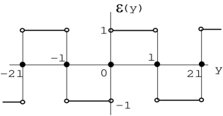
Figure 1: The graph of the periodic sign function $\epsilon(y)$, (32).

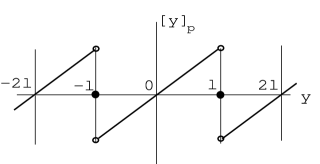
Figure 2: The graph of the sawtooth wave $[y]_{p}$, (36).

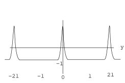
Figure 3: The graphs of the three distributions of (37). Top: Brane-Anti-Brane($B{\bar{B}}$); Middle: Anti-Brane(${\bar{B}}$); Bottom:   Brane($B$).

B) $Z_{2}$-even
The two independent solutions are given by the identity function (see Fig.4),

$$i(y)=\left\{\begin{array}[]{cc}1&-l<y\leq l\\ \mbox{periodic}&\mbox{other regions}\end{array}\right.{\quad.}$$ (40)

and the periodic ”absolute-linear” function (see Fig.5),

$$v(y)=\left\{\begin{array}[]{cc}|y|&-l<y\leq l\\ \mbox{periodic}&\mbox{other regions}\end{array}\right.{\quad.}$$ (43)

Both functions are continuous. The first one is smooth and the second one is piece-wise smooth. Their derivatives are given by

$$\frac{di(y)}{dy}=0{\quad,}\quad\frac{dv(y)}{dy}=\epsilon(y){\quad.}$$ (44)

The even solution $v(y)$ appears as the dilaton in the Randall-Sundrum of Sec.1. In the first example of Sec.1 and in the present model, the odd ones appear. The mathematical fact explained above shows the important connection among the brane configuration, the boundary condition and $Z_{2}$-symmetry.

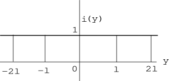
Figure 4: The graph of the identity function $i(y)$, (40).

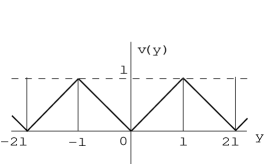
Figure 5: The graph of the periodic absolute-linear function $v(y)$, (43).

Let us examine the case 3) $a_{5\alpha}\propto Z_{\alpha}(\neq 0)$. Noting (27), we may put the following forms for $Z_{\alpha}$ and $a_{5\alpha}$.

$$Z_{\alpha}={\bar{Z}}_{\alpha}{\quad,}\quad a_{5\alpha}={\bar{a}}_{\alpha}j({x^{5}}){\quad,}\quad{\bar{Z}}_{\alpha}\propto{\bar{a}}_{\alpha}(\neq 0){\quad,}$$ (45)

where ${\bar{Z}}_{\alpha}$ and ${\bar{a}}_{\alpha}$ are constants and $j({x^{5}})$ is a function of ${x^{5}}$ which is to be specified below. The first equation of (45) says

$$-g(\delta({x^{5}})\eta^{\dagger}T^{\alpha}\eta+\delta({x^{5}}-l)\eta^{\prime{\dagger}}T^{\alpha}\eta^{\prime})-\partial_{5}\varphi_{\alpha}+g\,j({x^{5}})({\bar{a}}\times\varphi)_{\alpha}={\bar{Z}}_{\alpha}(\mbox{const}){\quad.}$$ (46)

The equation (19) says

$${\bar{a}}_{\alpha}{\partial_{5}}^{2}j-g(\varphi\times{\bar{Z}})_{\alpha}=0{\quad.}$$ (47)

First we solve (46) with the requirement:

$$\varphi_{\alpha}={\bar{\varphi}}_{\alpha}h({x^{5}}){\quad,}\quad{\bar{a}}_{\alpha}\propto{\bar{\varphi}}_{\alpha}{\quad,}$$ (48)

where ${\bar{\varphi}}_{\alpha}$ is a constant and $h({x^{5}})$ is a function of ${x^{5}}$ to be determined. The second relation says the two scalars, $a_{5}$ and $\varphi$, are (anti)parallel in the iso-space. Then (46) reduces to

$$-g(\delta({x^{5}})\eta^{\dagger}T^{\alpha}\eta+\delta({x^{5}}-l)\eta^{\prime{\dagger}}T^{\alpha}\eta^{\prime})-{\bar{\varphi}}_{\alpha}\partial_{5}h={\bar{Z}}_{\alpha}(\mbox{const}){\quad.}$$ (49)

From the equation (18), $h$ satisfies the ”free” field equation except the fixed points. Hence we have

$$h=c_{1}[{x^{5}}]_{p}+[{x^{5}}-l]_{p}{\quad,}$$

$${\bar{\varphi}}_{\alpha}=\frac{g}{2l}\eta^{\dagger}T^{\alpha}\eta=\frac{1}{c_{1}}\frac{g}{2l}\eta^{\prime{\dagger}}T^{\alpha}\eta^{\prime}{\quad,}$$

$$Z_{\alpha}=d_{\alpha}=-{\bar{\varphi}}_{\alpha}(1+c_{1})=-\frac{g}{2l}(1+c_{1})\eta^{\dagger}T^{\alpha}\eta{\quad.}$$ (50)

where $c_{1}$ is a free parameter. Next we solve (47). Because $\varphi_{\alpha}={\bar{\varphi}}_{\alpha}h({x^{5}})\propto{\bar{Z}}_{\alpha}$, the equation reduces to the ”free” one:

$${\bar{a}}_{\alpha}{\partial_{5}}^{2}j=0{\quad,}\quad{\bar{a}}_{\alpha}\neq 0{\quad.}$$ (51)

The solution is given by

$$j({x^{5}})=c_{2}[{x^{5}}]_{p}+[{x^{5}}-l]_{p}{\quad,}\quad\partial_{5}(\delta A_{5\alpha})|_{{x^{5}}=0,l}=0$$ (52)

where $c_{2}$ is another free parameter. Because ${\partial_{5}}^{2}j=-2lc_{2}\delta^{\prime}({x^{5}}-l)-2l\delta^{\prime}({x^{5}})$, the solution $j$ of (52), by itself, does not satisfy (51) on the points ${x^{5}}=0,l$. In order to correct it, we must require the variation $\delta A_{5\alpha}$, on the points ${x^{5}}=0,l$, to satisfy the Neumann boundary condition(the second relation of (52)). This condition ”absorbs” the singularities appearing in the variation equation (used to derive the field equation) at the points ${x^{5}}=0,l$ and makes the ”free” wave property (51) consistent everywhere in the extra space.

Summarizing the case 3) solution, we have

$$\varphi_{\alpha}={\bar{\varphi}}_{\alpha}\{c_{1}[{x^{5}}]_{p}+[{x^{5}}-l]_{p}\}{\quad,}\quad a_{5\alpha}={\bar{a}}_{\alpha}\{c_{2}[{x^{5}}]_{p}+[{x^{5}}-l]_{p}\}{\quad,}$$

$$\eta=\mbox{const}{\quad,}\quad\eta^{\prime}=\mbox{const}{\quad,}\quad{\bar{a}}_{\alpha}=c_{3}{\bar{\varphi}}_{\alpha}{\quad,}\quad{\bar{\varphi}}_{\alpha}=\frac{g}{2l}\eta^{\dagger}T^{\alpha}\eta=\frac{1}{c_{1}}\frac{g}{2l}\eta^{\prime{\dagger}}T^{\alpha}\eta^{\prime}{\quad,}$$

$$\chi^{3}_{\alpha}=-g\{\delta({x^{5}})+c_{1}\delta({x^{5}}-l)\}\eta^{\dagger}T^{\alpha}\eta\ ,\ Z_{\alpha}=d_{\alpha}=-\frac{g}{2l}(1+c_{1})\eta^{\dagger}T^{\alpha}\eta{\quad,}$$

$$\mbox{with the boundary condition: }\partial_{5}(\delta A_{5\alpha})|_{{x^{5}}=0,l}=0{\quad,}$$ (53)

where $c_{1},c_{2}$ and $c_{3}$ are three free parameters. The meaning of $c_{1}$ is the scale freedom in the ”parallel” condition of brane sources $\eta^{\prime{\dagger}}T^{\alpha}\eta^{\prime}\propto\eta^{\dagger}T^{\alpha}\eta$ , and that of $c_{2}$ and $c_{3}$ is the ”free” wave property of $a_{5\alpha}$ . The bulk scalar configuration influences the boundary source fields through the parameter $c_{1}$, whereas the bulk vector (5th component) does not have such effect. Instead the latter one satisfies the field equation only within the restricted variation (Neumann boundary condition).

This solution includes the cases 1) and 2) as described below. Some special cases are listed as follows.

(3A) $c_{3}=0$
This is the case 1). There are some special cases.

3A-a) $c_{1}=-1$
$\eta=\mbox{const}{\quad,}\quad\eta^{\prime}=\mbox{const}\ ,\ \eta^{\prime{\dagger}}T^{\alpha}\eta^{\prime}=-\,\eta^{\dagger}T^{\alpha}\eta\ ,$
$a_{5\alpha}=0\ ,\ \varphi_{\alpha}=-\frac{g}{2}\eta^{\dagger}T^{\alpha}\eta\,\epsilon({x^{5}})\ ,\ \chi^{3}_{\alpha}=-g(\delta({x^{5}})-\delta({x^{5}}-l))\eta^{\dagger}T^{\alpha}\eta\ ,$
$Z_{\alpha}=d_{\alpha}=0$

3A-b) $c_{1}=0$
$\eta=\mbox{const}{\quad,}\quad\eta^{\prime{\dagger}}T^{\alpha}\eta^{\prime}=0\ ,$
$a_{5\alpha}=0\ ,\ \varphi_{\alpha}=\frac{g}{2l}\eta^{\dagger}T^{\alpha}\eta[{x^{5}}-l]_{p}\ ,\ \chi^{3}_{\alpha}=-g\delta({x^{5}})\eta^{\dagger}T^{\alpha}\eta\ ,$
$Z_{\alpha}=d_{\alpha}=-\frac{g}{2l}\eta^{\dagger}T^{\alpha}\eta$

3A-c) $1/c_{1}\rightarrow 0$
$\eta^{\prime}=\mbox{const}{\quad,}\quad\eta^{\dagger}T^{\alpha}\eta=0\ ,$
$a_{5\alpha}=0\ ,\ \varphi_{\alpha}=\frac{g}{2l}\eta^{\prime{\dagger}}T^{\alpha}\eta^{\prime}[{x^{5}}]_{p}\ ,\ \chi^{3}_{\alpha}=-g\delta({x^{5}}-l)\eta^{\prime{\dagger}}T^{\alpha}\eta^{\prime}\ ,$
$Z_{\alpha}=d_{\alpha}=-\frac{g}{2l}\eta^{\prime{\dagger}}T^{\alpha}\eta^{\prime}$

3A-b) and 3A-c) are symmetric under the brane and anti-brane exchange. 3A-a) is self (anti)symmetric.

(3B) $c_{1}=-1$
This is the case 2).

(3C) $c_{1}=0$

(3D) $1/c_{1}\rightarrow 0$

(3E) $c_{2}=-1$
This is the case where the roles of the extra component of the bulk vector and the bulk scalar are exchanged in Case (3B).

(3F) $c_{2}=0$

(3G) $1/c_{2}\rightarrow 0$

Another special cases are given by fixing two parameters, $c_{1}$ and $c_{2}$ (keeping the $c_{3}$-freedom), as shown in Table 1.

$$\begin{array}[]{c|c|c|c}&\begin{array}[]{c}c_{2}=-1\\ \partial_{5}(\delta A_{5\alpha})|_{{x^{5}}=0,l}=0\end{array}&\begin{array}[]{c}c_{2}=0\\ \partial_{5}(\delta A_{5\alpha})|_{{x^{5}}=0}=0\end{array}&\begin{array}[]{c}c_{2}=1/0\\ \partial_{5}(\delta A_{5\alpha})|_{{x^{5}}=l}=0\end{array}\\ \hline\cr&&&\\ \begin{array}[]{c}c_{1}=-1\\ (\eta^{\prime{\dagger}}T^{\alpha}\eta^{\prime}\\ \ =-\eta^{\dagger}T^{\alpha}\eta)\end{array}&\begin{array}[]{c}\partial_{5}\varphi_{\alpha}:\ B{\bar{B}}\\ \partial_{5}a_{5\alpha}:\ B{\bar{B}}\\ d_{\alpha}=0\end{array}&\begin{array}[]{c}\partial_{5}\varphi_{\alpha}:\ B{\bar{B}}\\ \partial_{5}a_{5\alpha}:\ B\\ d_{\alpha}=0\end{array}&\begin{array}[]{c}\partial_{5}\varphi_{\alpha}:\ B{\bar{B}}\\ \partial_{5}a_{5\alpha}:\ {\bar{B}}\\ d_{\alpha}=0\end{array}\\ \hline\cr&&&\\ \begin{array}[]{c}c_{1}=0\\ (\eta^{\prime{\dagger}}T^{\alpha}\eta^{\prime}=0)\end{array}&\begin{array}[]{c}\partial_{5}\varphi_{\alpha}:\ B\\ \partial_{5}a_{5\alpha}:\ B{\bar{B}}\\ d_{\alpha}=-\frac{g}{2l}\eta^{\dagger}T^{\alpha}\eta\end{array}&\begin{array}[]{c}\partial_{5}\varphi_{\alpha}:\ B\\ \partial_{5}a_{5\alpha}:\ B\\ d_{\alpha}=-\frac{g}{2l}\eta^{\dagger}T^{\alpha}\eta\end{array}&\begin{array}[]{c}\partial_{5}\varphi_{\alpha}:\ B\\ \partial_{5}a_{5\alpha}:\ {\bar{B}}\\ d_{\alpha}=-\frac{g}{2l}\eta^{\dagger}T^{\alpha}\eta\end{array}\\ \hline\cr&&&\\ \begin{array}[]{c}c_{1}=1/0\\ (\eta^{\dagger}T^{\alpha}\eta=0)\end{array}&\begin{array}[]{c}\partial_{5}\varphi_{\alpha}:\ {\bar{B}}\\ \partial_{5}a_{5\alpha}:\ B{\bar{B}}\\ d_{\alpha}=-\frac{g}{2l}\eta^{\prime{\dagger}}T^{\alpha}\eta^{\prime}\end{array}&\begin{array}[]{c}\partial_{5}\varphi_{\alpha}:\ {\bar{B}}\\ \partial_{5}a_{5\alpha}:\ B\\ d_{\alpha}=-\frac{g}{2l}\eta^{\prime{\dagger}}T^{\alpha}\eta^{\prime}\end{array}&\begin{array}[]{c}\partial_{5}\varphi_{\alpha}:\ {\bar{B}}\\ \partial_{5}a_{5\alpha}:\ {\bar{B}}\\ d_{\alpha}=-\frac{g}{2l}\eta^{\prime{\dagger}}T^{\alpha}\eta^{\prime}\end{array}\\ \lx@intercol\hfil\hfil\lx@intercol\\ \lx@intercol\hfil\mbox{ Table\ 1\ \ Various vacuum configurations of the Mirabelli-Peskin model. }\hfil\lx@intercol\\ \lx@intercol\hfil\mbox{ \quad\quad\quad$B{\bar{B}}$, ${\bar{B}}$ and $B$ correspond to brane-anti-brane, anti-brane and brane }\hfil\lx@intercol\\ \lx@intercol\hfil\mbox{ \quad\quad\quad respectively. See Fig.3. }\hfil\lx@intercol\end{array}$$

We have solved only (18), (19) and (20). When $m_{{\alpha^{\prime}}{\beta^{\prime}}}$ and $\lambda_{{\alpha^{\prime}}{\beta^{\prime}}{\gamma^{\prime}}}$ are given, the equations (21) and (22) should be furthermore solved for $\eta,\eta^{\prime},f$ and $f^{\prime}$ using the obtained result. The solutions in the second row ($c_{1}=-1$) of Table 1 correspond to the SUSY invariant vacuum, irrespective of whether the vacuum expectation values of the brane-matter fields ($\eta$ and $\eta^{\prime}$) vanish or not. For other solutions, however, $d_{\alpha}$ depends on $\eta$ or $\eta^{\prime}$, hence the SUSY symmetry of the vacuum is determined by the brane-matter fields. The eqs. (21) and (22) have a ’trivial’ solution $\eta=0,f=0$ (or $\eta^{\prime}=0,f^{\prime}=0$) when $d_{\alpha}=-\frac{g}{2l}\eta^{\dagger}T^{\alpha}\eta$ (or $d_{\alpha}=-\frac{g}{2l}{\eta^{\prime}}^{\dagger}T^{\alpha}\eta^{\prime}$). It corresponds to the SUSY invariant vacuum. If the equations have a solution $\eta\neq 0$ (or $\eta^{\prime}\neq 0$), it corresponds to a SUSY-breaking vacuum.

We see the bulk scalar $\Phi$ is localized on the wall(s) where the source(s) exists, whereas the extra component of the bulk vector $A_{5}$ on the wall(s) where the Neumann boundary condition is imposed. The two cases, ($c_{1}=-1,c_{2}=-1$) and ($c_{1}=1/0,c_{2}=1/0$), are treated in [11].

4 Fermion Localization, Stability, and Bulk Higgs Mechanism The vacuum is basically determined by the scalar fields as explained so far. Let us examine the small fluctuation of bulk fermions (gauginos) around the background solution obtained previously. We take ($c_{1}=-1,c_{2}=-1$) solution as a representative one. We assume $\eta\neq 0,\eta^{\prime}\neq 0$. The relevant part of the Lagrangian is $-i{\bar{\lambda}}_{i}\gamma^{M}\nabla_{M}\lambda^{i}+g{\bar{\lambda}}_{i}[\Phi,\lambda^{i}]$. We consider a simple case of G=U(1). The field equation for $\lambda_{L}$ is given by

$$-i\{\gamma^{m}\partial_{m}\lambda_{L}+\gamma^{5}\partial_{5}\lambda_{L}-ga_{5}({x^{5}})\gamma^{5}\lambda_{L}\}+ig\varphi({x^{5}})\lambda_{L}=0{\quad,}$$

$$\varphi({x^{5}})=-\frac{g}{2}\eta^{\dagger}\eta\,\epsilon({x^{5}}){\quad,}\quad a_{5}({x^{5}})=c_{3}\varphi({x^{5}}){\quad.}$$ (54)

(The same thing can be said for $\lambda_{R}$.) We focus on the fermion zero-mode with chirality $\pm 1$: $\lambda_{L}=\sigma(x^{m})\omega({x^{5}}),\gamma^{m}\partial_{m}\sigma=0,\gamma^{5}\sigma=\pm\sigma$. Then the extra-space behaviour $\omega({x^{5}})$ is obtained as

$$\omega\propto\exp\{-\frac{g^{2}}{2}(1\pm c_{3})\eta^{\dagger}\eta\,|{x^{5}}|\}{\quad.}$$ (55)

As far as $1\pm c_{3}>0$, the fermion zero mode is localized around the brane. (If we require fermions with both chiralities to be localized, we must choose the parameter $c_{3}$ as $-1<c_{3}<1$.)

In the present approach, (${\cal N}=1$)SUSY is basically respected. If SUSY is preserved, the solutions obtained previously are expected to be stable, because the force between branes (Casimir force) vanish from the symmetry. In some cases, we can more strongly confirm the stableness from the topology (or index) as follows. We can regard the extra-space size ($S^{1}$ radius) $l$ as an infrared regularization parameter for the non-compact extra-space R($-\infty<y<\infty$). By letting $l\rightarrow+\infty$ in the previous result, we can obtain the vacuum solutions in this case. First we note

$$\epsilon(y)\rightarrow{\tilde{\epsilon}}(y){\quad,}\quad\frac{1}{l}[y]_{P}\rightarrow\frac{1}{l}y{\quad,}\quad\frac{1}{l}[y-l]_{P}=\frac{1}{l}[y]_{P}-\epsilon(y)\rightarrow\frac{1}{l}y-{\tilde{\epsilon}}(y){\quad,}$$

$$\frac{d\epsilon(y)}{dy}\rightarrow 2{\tilde{\delta}}(y){\quad,}\quad\frac{1}{l}\frac{d}{dy}[y]_{P}\rightarrow 0{\quad,}\quad\frac{1}{l}\frac{d}{dy}[y-l]_{P}\rightarrow-2{\tilde{\delta}}(y){\quad,}$$

$$\mbox{ as }l\rightarrow\infty{\quad.}\quad\quad\quad\quad\quad$$ (56)

An interesting case is the $l\rightarrow\infty$ limit of ($c_{1}=-1,c_{2}=-1$) in Table 1.

$$\varphi_{\alpha}=-{\bar{\varphi}}_{\alpha}l\epsilon({x^{5}})\rightarrow-\frac{g}{2}\eta^{\dagger}T^{\alpha}\eta{\tilde{\epsilon}}({x^{5}}){\quad,}\quad a_{5\alpha}=-{\bar{a}}_{\alpha}l\epsilon({x^{5}})\rightarrow-c_{3}\frac{g}{2}\eta^{\dagger}T^{\alpha}\eta{\tilde{\epsilon}}({x^{5}}){\quad,}$$

$$\chi^{3}_{\alpha}=-g\delta({x^{5}})\eta^{\dagger}T^{\alpha}\eta{\quad,}\quad Z_{\alpha}=d_{\alpha}=0{\quad,}$$

$$\mbox{with the boundary condition: }\partial_{5}(\delta A_{5\alpha})|_{{x^{5}}=0}=0{\quad.}$$ (57)

Indeed we can confirm the above limit is a solution of

$$S=\int d^{4}x\int_{-\infty}^{+\infty}dx^{5}\{{\cal L}_{blk}+{\tilde{\delta}}(x^{5}){\cal L}_{bnd}\}{\quad,}\quad-\infty<{x^{5}}<\infty{\quad,}$$ (58)

where ${\cal L}_{blk}$ and ${\cal L}_{bnd}$ are the same as in Sec.2 except that fields are no more periodic. The stableness is clear from the same situation as the kink solution of Sec.1. On the other hand, in the $l\rightarrow\infty$ limit of ($c_{1}=1/0,c_{2}=1/0$) there remains no localization configuration.

As a bulk Higgs model, which embodies the non-singular treatment (kink-generalization) of the singular solution, (57) and (58), we can present the following one. We make use of the ${\cal N}=1$ chiral superfield[9]: $\Sigma=\Phi+iA_{5}+\sqrt{2}\theta(-i\sqrt{2}\lambda_{R})+\theta^{2}(X^{1}+iX^{2})$, which appears, along with ${\cal N}=1$ vector multiplet, in the $Z_{2}$-parity decomposition explained in Sec.2. We propose the following model.

$$S=\int_{-\infty}^{\infty}d{x^{5}}\int d^{4}x\{{\cal L}_{blk}+(P(\Sigma)|_{\theta^{2}}+\mbox{h.c.})+{\cal L}_{matter}\}{\quad,}$$

$$P(\Sigma)=m^{2}\Sigma-\frac{\lambda}{3}\Sigma^{3}{\quad,}$$ (59)

where $m$ and $\lambda$ are a mass parameter and a (dimensionless) coupling constant respectively. ${\cal L}_{matter}$ is the matter lagrangian made of the 5D SUSY hypermultiplet[9]: $H^{1},H^{2}$, two complex scalar fields; $\Psi$, one Dirac field; $F_{1},F_{2}$, two auxiliary fields. The brane thickness parameter is given by $m/\sqrt{\lambda}$ as a vacuum expectation value of $\Phi+iA_{5}$. In this model, the complex scalar field in the chiral multiplet plays the role of ”radion” although the present ”radion” determines not the extra-space size ( $l\rightarrow\infty$ in the present model) but the brane thickness. We expect the above model gives a non-singular brane solution (kink solution in the extra-space) which is both stable and supersymmetric.

5 Conclusion In the brane system appearing in string/D-brane theory, the stableness is the most important requirement. We find some stable brane configurations in the SUSY bulk-boundary theory. We systematically solve the singular field equation using a general mathematical result about the free-wave solution in $S_{1}/Z_{2}$-space. The two scalars, the extra-component of the bulk-vector ($A_{5}$) and the bulk-scalar($\Phi$), constitute the solutions. Their different roles are clarified. The importance of the ”parallel” configuration is disclosed. The boundary condition (of $A_{5}$) and the boundary matter fields are two important elements for making the localized configuration. Among all solutions, the solution ($c_{1}=-1,c_{2}=-1$) is expected to be the thin-wall limit of a kink solution. We present a bulk Higgs model corresponding to the non-singular solution. The model is expected to give a non-singular and stable brane solution in the SUSY bulk-boundary theory.

In ref.[11, 10], the 1-loop effective potential is obtained for the backgrounds $(c_{1}=-1,c_{2}=-1)$. In ref.[12], a bulk effect in the 1-loop effective potential is analyzed in relation to the SUSY breaking. We hope the family of present solutions will be used for further understanding of the bulk-boundary system.

References

[1] R. Rajaraman,
Solitons and instantons, North-Holland Pub., Amsterdam,C1982
[2] L.Randall and R.Sundrum,
Phys.Rev.Lett.83(1999)3370,hep-ph/9905221
[3] L.Randall and R.Sundrum,
Phys.Rev.Lett.83(1999)4690,hep-th/9906064
[4] W. Goldberger and M. Wise, Phys.Rev.D60(1999)107505; Phys.Rev.Lett.83(1999)4922
[7] P.Hořava and E.Witten,
Nucl.Phys.B460(1996)506,hep-th/9510209
[8] E.A.Mirabelli and M.E. Peskin,
Phys.Rev.D58(1998)065002, hep-th/9712214
[9] A. Hebecker, Nucl.Phys.B632(2002)101
[10] S. Ichinose and A. Murayama, hep-th/0401011, US-03-08
”Quantum Dynamics of A Bulk-Boundary System”
[11] S. Ichinose and A. Murayama, hep-th/0302029,
Phys.Lett.B587(2004)121
[12] S. Ichinose and A. Murayama, hep-th/0403080, US-03-07,
to be published in Phys.Lett.B.
”A Bulk Effect to SUSY Effective Potential in a 5D Super-Yang-Mills Model”