Inflation, quantum fluctuations and cosmological perturbations

Abstract

These lectures are intended to give a pedagogical introduction to the main current picture of the very early universe. After elementary reviews of general relativity and of the standard Big Bang model, the following subjects are discussed: inflation, the classical relativistic theory of cosmological perturbations and the generation of perturbations from scalar field quantum fluctuations during inflation.

1 Introduction

The purpose of these lectures is to give an introduction to the present standard picture of the early universe, which complements the older standard Big Bang model. These notes are intended for non-experts on this subject. They start with a very short introduction to General Relativity, on which modern cosmology is based, followed by an elementary review of the standard Big Bang model. We then discuss the limitations of this model and enter into the main subject of these lectures: inflation.

Inflation was initially invented to solve some of the problems of the standard Big Bang model and to get rid of unwanted relics generically predicted by high energy models. It turned out that inflation, as it was realized later, could also solve an additional puzzle of the standard model, that of the generation of the cosmological perturbations. This welcome surprise put inflation on a rather firm footing, about twenty years ago. Twenty years later, inflation is still alive, in a stronger position than ever because its few competitors have been eliminated as new cosmological observations have accumulated during the last few years.

2 A few elements on general relativity and cosmology

Modern cosmology is based on Einstein’s theory of general relativity. It is thus useful, before discussing the early universe, to recall a few notions and useful formulas from this theory. Details can be found in standard textbooks on general relativity (see e.g. [1]). In the framework of general relativity, the spacetime geometry is defined by a metric, a symmetric tensor with two indices, whose components in a coordinate system $\{x^{\mu}\}$ ($\mu=0,1,2,3$) will be denoted $g_{\mu\nu}$. The square of the “distance” between two neighbouring points of spacetime is given by the expression

$$ds^{2}=g_{\mu\nu}dx^{\mu}dx^{\nu}.$$ (1)

We will use the signature $(-,+,+,+)$.

In a coordinate change $x^{\mu}\rightarrow\tilde{x}^{\mu}$, the new components of the metric are obtained by using the standard tensor transformation formulas, namely

$$\tilde{g}_{\mu\nu}={\partial x^{\rho}\over\partial\tilde{x}^{\mu}}{\partial x^{\sigma}\over\partial\tilde{x}^{\nu}}g_{\rho\sigma}.$$ (2)

One can define a covariant derivative associated to this metric, denoted $D_{\mu}$, whose action on a tensor with, for example, one covariant index and one contravariant index will be given by

$$D_{\lambda}T^{\mu}_{\hskip 5.69054pt\nu}=\partial_{\lambda}T^{\mu}_{\hskip 5.69054pt\nu}+\Gamma^{\mu}_{\lambda\sigma}T^{\sigma}_{\hskip 5.69054pt\nu}-\Gamma^{\sigma}_{\lambda\nu}T^{\mu}_{\hskip 5.69054pt\sigma}$$ (3)

(a similar term must be added for each additional covariant or contravariant index), where the $\Gamma$ are the Christoffel symbols (they are not tensors), defined by

$$\Gamma^{\lambda}_{\mu\nu}={1\over 2}g^{\lambda\sigma}\left(\partial_{\mu}g_{\sigma\nu}+\partial_{\nu}g_{\mu\sigma}-\partial_{\sigma}g_{\mu\nu}\right).$$ (4)

We have used the notation $g^{\mu\nu}$ which corresponds, for the metric (and only for the metric), to the inverse of $g_{\mu\nu}$ in a matricial sense, i.e. $g_{\mu\sigma}g^{\sigma\nu}=\delta_{\mu}^{\nu}$.

The “curvature” of spacetime is characterized by the Riemann tensor, whose components can be expressed in terms of the Christoffel symbols according to the expression

$$R_{\lambda\mu\nu}^{\hskip 17.07164pt\rho}=\partial_{\mu}\Gamma_{\lambda\nu}^{\rho}-\partial_{\lambda}\Gamma_{\mu\nu}^{\rho}+\Gamma_{\lambda\nu}^{\sigma}\Gamma_{\sigma\mu}^{\rho}-\Gamma_{\mu\nu}^{\sigma}\Gamma_{\sigma\lambda}^{\rho}.$$ (5)

Einstein’s equations relate the spacetime geometry to its matter content. The geometry appears in Einstein’s equations via the Ricci tensor, defined by

$$R_{\mu\nu}=R_{\mu\sigma\nu}^{\hskip 17.07164pt\sigma},$$ (6)

and the scalar curvature, which is the trace of the Ricci tensor, i.e.

$$R=g^{\mu\nu}R_{\mu\nu}.$$ (7)

The matter enters Einstein’s equations via the energy-momentum tensor, denoted $T_{\mu\nu}$, whose time/time component corresponds to the energy density, the time/space components to the momentum density and the space/space component to the stress tensor. Einstein’s equations then read

$$G_{\mu\nu}\equiv R_{\mu\nu}-{1\over 2}R\,g_{\mu\nu}=8\pi G\,T_{\mu\nu},$$ (8)

where the tensor $G_{\mu\nu}$ is called the Einstein tensor. Since, by construction, the Einstein tensor satisfies the identity $D_{\mu}G^{\mu}_{\,\nu}=0$, any energy-momentum on the right-hand side of Einstein’s equation must necessarily satisfy the relation

$$D_{\mu}T^{\mu}_{\,\nu}=0,$$ (9)

which can be interpreted as a generalization, in the context of a curved spacetime, of the familiar conservation laws for energy and momentum.

The motion of a particule is described by its trajectory in spacetime, $x^{\mu}(\lambda)$, where $\lambda$ is a parameter. A free particle, i.e. which does not feel any force (other than gravity), satisfies the geodesic equation, which reads

$$t^{\sigma}D_{\sigma}t^{\mu}=0,$$ (10)

where $t^{\mu}=dx^{\mu}/d\lambda$ is the vector field tangent to the trajectory (note that the geodesic equation written in this form assumes that the parameter $\lambda$ is affine). Equivalently, the geodesic can be rewritten as

$${d^{2}x^{\mu}\over d\lambda^{2}}+\Gamma^{\mu}_{\rho\sigma}{dx^{\rho}\over d\lambda}{dx^{\sigma}\over d\lambda}=0.$$ (11)

The geodesic equation applies both to

• massive particles, in which case one usually takes as the parameter $\lambda$ the so-called proper time so that the corresponding tangent vector $u^{\mu}$ is normalized: $g_{\mu\nu}u^{\mu}u^{\nu}=-1$;

• massless particles, in particular the photon, in which case the tangent vector, usually denoted $k^{\mu}$ is light-like, i.e. $g_{\mu\nu}k^{\mu}k^{\nu}=0$.

Einstein’s equations can also be obtained from a variational principle. The corresponding action reads

$${\cal S}={1\over 16\pi G}\int d^{4}x\sqrt{-g}\left(R-2\Lambda\right)+\int d^{4}x\sqrt{-g}{\cal L}_{mat}.$$ (12)

One can check that the variation of this action with respect to the metric $g_{\mu\nu}$ , upon using the definition

$$T^{\mu\nu}={2\over\sqrt{-g}}{\delta\left(\sqrt{-g}{\cal L}_{mat}\right)\over{\delta g_{\mu\nu}}},$$ (13)

indeed gives Einstein’s equations

$$G_{\mu\nu}+\Lambda g_{\mu\nu}=8\pi G\,T_{\mu\nu}.$$ (14)

This is a slight generalization of Einstein’s equations (8) that includes a cosmological constant $\Lambda$. It is worth noticing that the cosmological constant can also be interpreted as a particular energy-momentum tensor of the form $T_{\mu\nu}=-(8\pi G)^{-1}\Lambda g_{\mu\nu}$.

2.1 Review of standard cosmology

In this subsection, the foundations of modern cosmology are briefly recalled. They follow from Einstein’s equations introduced above and from a few hypotheses concerning spacetime and its matter content. One of the essential assumptions of cosmology (so far confirmed by observations) is to consider, as a first approximation, the universe as being homogeneous and isotropic. Note that these symmetries define implicitly a particular “slicing” of spacetime, the corresponding space-like hypersurfaces being homogeneous and isotropic. A different slicing of the same spacetime will give in general space-like hypersurfaces that are not homogeneous and isotropic.

The above hypothesis turns out to be very restrictive and the only metrics compatible with this requirement reduce to the so-called Robertson-Walker metrics, which read in an appropriate coordinate system

$$ds^{2}=-dt^{2}+a^{2}(t)\left[{dr^{2}\over{1-\kappa r^{2}}}+r^{2}\left(d\theta^{2}+\sin^{2}\theta d\phi^{2}\right)\right],$$ (15)

with $\kappa=0,-1,1$ depending on the curvature of spatial hypersurfaces: respectively flat, elliptic or hyperbolic.

The matter content compatible with the spacetime symmetries of homogeneity and isotropy is necessarily described by an energy-momentum tensor of the form (in the same coordinate system as for the metric (15)):

$$T^{\mu}_{\,\nu}={\rm Diag}\left(-\rho(t),p(t),p(t),p(t)\right).$$ (16)

The quantity $\rho$ corresponds to an energy density and $P$ to a pressure.

One can show that the so-called comoving particles, i.e. those particles whose spatial coordinates are constant in time, satisfy the geodesic equation (11).

2.2 Friedmann-Lemaître equations

Substituting the Robertson-Walker metric (15) in Einstein’s equations (8), one gets the so-called Friedmann-Lemaître equations:

$$\left({\dot{a}\over a}\right)^{2} = {8\pi G\rho\over 3}-{\kappa\over a^{2}},$$ (17)

$${\ddot{a}\over a} = -{4\pi G\over 3}\left(\rho+3P\right).$$ (18)

An immediate consequence of these two equations is the continuity equation

$$\dot{\rho}+3H\left(\rho+p\right)=0,$$ (19)

where $H\equiv\dot{a}/a$ is the Hubble parameter. The continuity equation can be also obtained directly from the energy-momentum conservation $D_{\mu}T^{\mu}_{\,\nu}=0$, as mentioned before.

In order to determine the cosmological evolution, it is easier to combine (17) with (19). Let us assume an equation of state for the cosmological matter of the form $p=w\rho$ with $w$ constant. This includes the two main types of matter that play an important rôle in cosmology:

• gas of relativistic particles, $w=1/3$;

• non relativistic matter, $w\simeq 0$.

In these cases, the conservation equation (19) can be integrated to give

$$\rho\propto a^{-3(1+w)}.$$ (20)

Substituting in (17), one finds, for $\kappa=0$,

$$3{\dot{a}^{2}\over a^{2}}=8\pi G\rho_{0}\left(a\over a_{0}\right)^{-3(1+w)},$$ (21)

where, by convention, the subscript ’0’ stands for present quantities. One thus finds $\dot{a}^{2}\propto a^{2-3(1+w)}$, which gives for the evolution of the scale factor

• in a universe dominated by non relativistic matter

  $$a(t)\propto t^{2/3},$$ (22)

• and in a universe dominated by radiation

  $$a(t)\propto t^{1/2}.$$ (23)

One can also mention the case of a cosmological constant, which corresponds to an equation of state $w=-1$ and thus implies an exponential evolution for the scale factor

$$a(t)\propto\exp(Ht).$$ (24)

More generally, when several types of matter coexist with respectively $p_{(i)}=w_{(i)}\rho_{(i)}$, it is convenient to introduce the dimensionless parameters

$$\Omega_{(i)}={8\pi G\rho_{0}^{(i)}\over 3H_{0}^{2}},$$ (25)

which express the present ratio of the energy density of some given species with respect to the so-called critical energy density $\rho_{crit}=3H_{0}^{2}/(8\pi G)$, which corresponds to the total energy density for a flat universe.

One can then rewrite the first Friedmann equation (17) as

$$\left({H\over H_{0}}\right)^{2}=\sum_{i}\Omega_{(i)}\left(a\over a_{0}\right)^{-3(1+w_{(i)})}+\Omega_{\kappa}\left(a\over a_{0}\right)^{-2},$$ (26)

with $\Omega_{\kappa}=-\kappa/a_{0}^{2}H_{0}^{2}$, which implies that the cosmological parameters must satisfy the consistency relation

$$\sum_{i}\Omega_{(i)}+\Omega_{\kappa}=1.$$ (27)

As for the second Friedmann equation (18), it implies

$${\ddot{a}_{0}\over a_{0}H_{0}^{2}}=-{1\over 2}\sum_{i}\Omega_{(i)}(1+w_{(i)}).$$ (28)

Present cosmological observations yield for the various parameters

• Baryons: $\Omega_{b}\simeq 0.05$,

• Dark matter: $\Omega_{d}\simeq 0.25$,

• Dark energy (compatible with a cosmological constant): $\Omega_{\Lambda}\simeq 0.7$,

• Photons: $\Omega_{\gamma}\simeq 5\times 10^{-5}$.

Observations have not detected so far any deviation from flatness. Radiation is very subdominant today but extrapolating backwards in time, radiation was dominant in the past since its energy density scales as $\rho_{\gamma}\propto a^{-4}$ in contrast with non relativistic matter ($\rho_{m}\propto a^{-3}$). Moreover, since the present matter content seems dominated by dark energy similar to a cosmological constant ($w_{\Lambda}=-1$), this indicates that our universe is presently accelerating.

2.3 The cosmological redshift

An important consequence of the expansion of the universe is the cosmological redshift of photons. This is in fact how the expansion of the universe was discovered initially.

Let us consider two light signals emitted by a comoving object at two successive instants $t_{e}$ and $t_{e}+\delta t_{e}$, then received later at respectively $t_{o}$ and $t_{o}+\delta t_{o}$ by a (comoving) observer. One can always set the observer at the center of the coordinate system. All light trajectories reaching the observer are then radial and one can write, using (15)

$$\int_{0}^{r_{e}}{dr\over\sqrt{1-\kappa r^{2}}}=\int_{t_{e}}^{t_{o}}{dt\over a(t)}.$$ (29)

The left-hand side being identical for the two successive trajectories, the right-hand side must vanish, which yields

$${\delta t_{o}\over a_{o}}-{\delta t_{e}\over a_{e}}=0.$$ (30)

This implies for the frequencies measured at emission and at reception a redshift given by

$$1+z\equiv{\nu_{e}\over\nu_{o}}={a_{o}\over a_{e}}.$$ (31)

2.4 Thermal history of the universe

To go beyond a simply geometrical description of cosmology, it is very fruitful to apply thermodynamics to the matter content of the universe. One can then define a temperature $T$ for the cosmological photons, not only when they are strongly interacting with ordinary matter but also after they have decoupled because, with the expansion, the thermal distribution for the gas of photons is unchanged except for a global rescaling of the temperature so that $T$ essentially evolves as

$$T(t)\propto{1\over a(t)}.$$ (32)

This means that, going backwards in time, the universe was hotter and hotter. This is the essence of the hot Big Bang scenario.

As the universe evolves, the reaction rates between the various species are modified. A detailed analysis of these changes enables to reconstruct the past thermal history of the universe. Two events in particular play an essential rôle because of their observational consequences:

• Primordial nucleosynthesis

  Nucleosynthesis occured at a temperature around $0.1$ MeV, when the average kinetic energy became sufficiently low so that nuclear binding was possible. Protons and neutrons could then combine, which lead to the production of light elements, such that Helium, Deuterium, Lithium, etc… Within the observational uncertainties, this scenario is remarkably confirmed by the present measurements.

• Decoupling of baryons and photons (or last scattering)

  A more recent event is the so-called “recombination” of nuclei and electrons to form atoms. This occured at a temperature of the order of the eV. Free electrons thus almost disappeared, which entailed an effective decoupling of the cosmological photons and ordinary matter. What we see today as the Cosmic Microwave Background (CMB) is made of the fossil photons, which interacted for the last time with matter at the last scattering epoch. The CMB represents a remarkable observational tool for analysing the perturbations of the early universe, as well as for measuring the cosmological parameters introduced above.

2.5 Puzzles of the standard Big Bang model

The standard Big Bang model has encountered remarkable successes, in particular with the nucleosynthesis scenario and the prediction of the CMB, and it remains today a cornerstone in our understanding of the present and past universe. However, a few intriguing facts remain unexplained in the strict scenario of the standard Big Bang model and seem to necessitate a larger framework. We review below the main problems:

• Homogeneity problem

  A first question is why the approximation of homogeneity and isotropy turns out to be so good. Indeed, inhomogeneities are unstable, because of gravitation, and they tend to grow with time. It can be verified for instance with the CMB that inhomogeneities were much smaller at the last scattering epoch than today. One thus expects that these homogeneities were still smaller further back in time. How to explain a universe so smooth in its past ?

• Flatness problem

  Another puzzle lies in the (spatial) flatness of our universe. Indeed, Friedmann’s equation (17) implies

  $$\Omega-1\equiv{8\pi G\rho\over 3H^{2}}-1={\kappa\over a^{2}H^{2}}.$$ (33)

  In standard cosmology, the scale factor behaves like $a\sim t^{p}$ with $p<1$ ($p=1/2$ for radiation and $p=2/3$ for non-relativistic matter). As a consequence, $(aH)^{-2}$ grows with time and $|\Omega-1|$ must thus diverge with time. Therefore, in the context of the standard model, the quasi-flatness observed today requires an extreme fine-tuning of $\Omega$ near $1$ in the early universe.

• Horizon problem

  

  Figure 1: Evolution of the comoving Hubble radius $\lambda_{H}=(aH)^{-1}$: during standard cosmology, $\lambda_{H}$ increases (continuous lines), whereas during inflation $\lambda_{H}$ shrinks (dashed lines).

  One of the most fundamental problems in standard cosmology is certainly the horizon problem. The (particle) horizon is the maximal distance that can be covered by a light ray. For a light-like radial trajectory $dr=a(t)dt$ and the horizon is thus given by

  $$d_{H}(t)=a(t)\int_{t_{i}}^{t}{dt^{\prime}\over a(t^{\prime})}=a(t){t^{1-q}-t_{i}^{1-q}\over 1-q},$$ (34)

  where the last equality is obtained by assuming $a(t)\sim t^{q}$ and $t_{i}$ is some initial time.

  In standard cosmology ($q<1$), the integral converges in the limit $t_{i}=0$ and the horizon has a finite size, of the order of the so-called Hubble radius $H^{-1}$:

  $$d_{H}(t)={q\over 1-q}H^{-1}.$$ (35)

  It also useful to consider the comoving Hubble radius, $(aH)^{-1}$, which represents the fraction of comoving space in causal contact. One finds that it grows with time, which means that the fraction of the universe in causal contact increases with time in the context of standard cosmology. But the CMB tells us that the Universe was quasi-homogeneous at the time of last scattering on a scale encompassing many regions a priori causally independent. How to explain this ?

A solution to the horizon problem and to the other puzzles is provided by the inflationary scenario, which we will examine in the next section. The basic idea is to invert the behaviour of the comoving Hubble radius, that is to make him decrease sufficiently in the very early universe. The corresponding condition is that

$$\ddot{a}>0,$$ (36)

i.e. that the Universe must undergo a phase of acceleration.

3 Inflation

The broadest definition of inflation is that it corresponds to a phase of acceleration of the universe,

$$\ddot{a}>0.$$ (37)

In this broad sense, the current cosmological observations, if correctly interpreted, mean that our present universe is undergoing an inflationary phase. We are however interested here in an inflationary phase taking place in the very early universe, with different energy scales.

The Friedmann equations (17) tell us that one can get acceleration only if the equation of state satisfies the condition

$$P<-{1\over 3}\rho,$$ (38)

condition which looks at first view rather exotic.

A very simple example giving such an equation of state is a cosmological constant, corresponding to a cosmological fluid with the equation of state

$$P=-\rho.$$ (39)

However, a strict cosmological constant leads to exponential inflation forever which cannot be followed by a radiation or matter era. Another possibility is a scalar field, which we discuss now in some details.

3.1 Cosmological scalar fields

The dynamics of a scalar field coupled to gravity is governed by the action

$$S_{\phi}=\int d^{4}x\sqrt{-g}\left(-{1\over 2}\partial^{\mu}\phi\partial_{\mu}\phi-V(\phi)\right).$$ (40)

The corresponding energy-momentum tensor, which can be derived using (13), is given by

$$T_{\mu\nu}=\partial_{\mu}\phi\partial_{\nu}\phi-g_{\mu\nu}\left({1\over 2}\partial^{\sigma}\phi\partial_{\sigma}\phi+V(\phi)\right).$$ (41)

If one assumes the geometry, and thus the matter, to be homogeneous and isotropic, then the energy-momentum tensor reduces to the perfect fluid form with the energy density

$$\rho=-T_{0}^{0}={1\over 2}\dot{\phi}^{2}+V(\phi),$$ (42)

where one recognizes the sum of a kinetic energy and of a potential energy, and the pressure

$$p={1\over 2}\dot{\phi}^{2}-V(\phi).$$ (43)

The equation of motion for the scalar field is the Klein-Gordon equation, which is obtained by taking the variation of the above action (40) with respect to the scalar field and which reads

$$D^{\mu}D_{\mu}\phi=V^{\prime},$$ (44)

in general and

$$\ddot{\phi}+3H\dot{\phi}+V^{\prime}=0$$ (45)

in the particular case of a FLRW (Friedmann-Lemaître-Robertson-Walker) universe.

The system of equations governing the dynamics of the scalar field and of the geometry in a FLRW universe is thus given by

$$H^{2}={8\pi G\over 3}\left({1\over 2}\dot{\phi}^{2}+V(\phi)\right),$$ (46)

$$\ddot{\phi}+3H\dot{\phi}+V^{\prime}=0,$$ (47)

$$\dot{H}=-4\pi G\dot{\phi}^{2}.$$ (48)

The last equation can be derived from the first two and is therefore redundant.

3.2 The slow-roll regime

The dynamical system (46-48) does not always give an accelerated expansion but it does so in the so-called slow-roll regime when the potential energy of the scalar field dominates over its kinetic energy.

More specifically, the so-called slow roll approximation consists in neglecting the kinetic energy of the scalar field , $\dot{\phi}^{2}/2$ in (46) and the acceleration $\ddot{\phi}$ in the Klein-Gordon equation (47). One then gets the simplified system

$$H^{2}\simeq{8\pi G\over 3}V,$$ (49)

$$3H\dot{\phi}+V^{\prime}\simeq 0.$$ (50)

Let us now examine in which regime this approximation is valid. From (50), the velocity of the scalar field is given by

$$\dot{\phi}\simeq-{V^{\prime}\over 3H}.$$ (51)

Substituting this relation in the condition $\dot{\phi}^{2}/2\ll V$ yields the requirement:

$$\epsilon_{V}\equiv{m_{P}^{2}\over 2}\left({V^{\prime}\over V}\right)^{2}\ll 1,$$ (52)

where we have introduced the reduced Planck mass

$$m_{P}\equiv{1\over\sqrt{8\pi G}}.$$ (53)

Similarly, the time derivative of (51), using the time derivative of (49), gives, after substitution in $\ddot{\phi}\ll V^{\prime}$, the condition

$$\eta_{V}\equiv m_{P}^{2}{V^{\prime\prime}\over V}\ll 1.$$ (54)

In summary, the slow-roll approximation is valid when the two conditions $\epsilon_{V},\eta_{V}\ll 1$ are satisfied, which means that the slope and the curvature of the potential, in Planck units, must be sufficiently small.

3.3 Number of e-folds

When working with a specific inflationary model, it is important to be able to relate the cosmological scales observed at the present time with the scales during inflation. For this purpose, one usally introduces the number of e-foldings before the end of inflation, denoted $N$, and simply defined by

$$N=\ln{a_{end}\over a},$$ (55)

where $a_{end}$ is the value of the scale factor at the end of inflation and $a$ is a fiducial value for the scale factor during inflation. By definition, $N$ decreases during the inflationary phase and reaches zero at its end. In the slow-roll approximation, it is possible to express $N$ as a function of the scalar field. Since $dN=-d\ln a=-Hdt=-(H/\dot{\phi})d\phi$, one easily finds, using (51) and (49), that

$$N(\phi)\simeq\int_{\phi}^{\phi_{end}}{V\over m_{P}^{2}V^{\prime}}d\phi.$$ (56)

Given an explicit potential $V(\phi)$, one can in principle integrate the above expression to obtain $N$ in terms of $\phi$. This will be illustrated below for some specific models.

Let us now discuss the link between $N$ and the present cosmological scales. Let us consider a given scale characterized by its comoving wavenumber $k=2\pi/\lambda$. This scale crossed outside the Hubble radius, during inflation, at an instant $t_{*}(k)$ defined by

$$k=a(t_{*})H(t_{*}).$$ (57)

To get a rough estimate of the number of e-foldings of inflation that are needed to solve the horizon problem, let us first ignore the transition from a radiation era to a matter era and assume for simplicity that the inflationary phase was followed instantaneously by a radiation phase that has lasted until now. During the radiation phase, the comoving Hubble radius $(aH)^{-1}$ increases like $a$. In order to solve the horizon problem, the increase of the comoving Hubble radius during the standard evolution must be compensated by at least a decrease of the same amount during inflation. Since the comoving Hubble radius roughly scales like $a^{-1}$ during inflation, the minimum amount of inflation is simply given by the number of e-folds between the end of inflation and today $\ln(a_{0}/a_{end})=\ln(T_{end}/T_{0})\sim\ln(10^{29}(T_{end}/10^{16}{\rm GeV}))$, i.e. around 60 e-folds for a temperature $T\sim 10^{16}{\rm Gev}$ at the beginning of the radiation era. As we will see later, this energy scale is typical of inflation in the simplest models.

This determines roughly the number of e-folds $N(k_{0})$ between the moment when the scale corresponding to our present Hubble radius $k_{0}=a_{0}H_{0}$ exited the Hubble radius during inflation and the end of inflation. The other lengthscales of cosmological interest are smaller than $k_{0}^{-1}$ and therefore exited the Hubble radius during inflation after the scale $k_{0}$, whereas they entered the Hubble radius during the standard cosmological phase (either in the radiation era for the smaller scales or in the matter era for the larger scales) before the scale $k_{0}$.

A more detailed calculation, which distinguishes between the energy scales at the end of inflation and after the reheating, gives for the number of e-folds between the exit of the mode $k$ and the end of inflation

$$N(k)\simeq 62-\ln{k\over a_{0}H_{0}}+\ln{V_{k}^{1/4}\over 10^{16}{\rm GeV}}+\ln{V_{k}^{1/4}\over V_{\rm end}^{1/4}}+{1\over 3}\ln{\rho_{\rm reh}^{1/4}\over V_{\rm end}^{1/4}}.$$ (58)

Since the smallest scale of cosmological relevance is of the order of $1$ Mpc, the range of cosmological scales covers about $9$ e-folds.

The above number of e-folds is altered if one changes the thermal history of the universe between inflation and the present time by including for instance a period of so-called thermal inflation.

3.4 Power-law potentials

It is now time to illustrate all the points discussed above with some specific potential. We consider first the case of power-law monomial potentials, of the form

$$V(\phi)={\lambda\over p}m_{P}^{4}\left({\phi\over m_{P}}\right)^{p},$$ (59)

which have been abundantly used in the literature. In particular, the above potential includes the case of a free massive scalar field, $V(\phi)=m^{2}\phi/2$. The slow-roll conditions $\epsilon\ll 1$ and $\eta\ll 1$ both imply

$$\phi\gg p\ m_{P},$$ (60)

which means that the scalar field amplitude must be above the Planck mass during inflation.

After subsituting the potential (59) into the slow-roll equations of motion (49-50), one can integrate them explicitly to get

$$\phi^{2-{p\over 2}}-\phi_{i}^{2-{p\over 2}}=-{2\over 4-p}\,\sqrt{p\lambda\over 3}\,m_{P}^{3-{p\over 2}}\left(t-t_{i}\right)$$ (61)

for $p\neq 4$ and

$$\phi=\phi_{i}\exp\left[-\sqrt{4\lambda\over 3}\,m_{P}(t-t_{i})\right]$$ (62)

for $p=4$.

One can also express the scale factor as a function of the scalar field (and thus as a function of time by substituting the above expression for $\phi(t)$) by using $d\ln a/d\phi=H/\dot{\phi}\simeq-\phi/(pm_{P}^{2})$. One finds

$$a=a_{end}\exp\left[-{\left(\phi^{2}-\phi_{end}^{2}\right)\over 2p\,m_{P}^{2}}\right].$$ (63)

Defining the end of inflation by $\epsilon_{V}=1$, one gets $\phi_{end}=p\,m_{P}/\sqrt{2}$ and the number of e-folds is thus given by

$$N(\phi)\simeq{\phi^{2}\over 2pm_{P}^{2}}-{p\over 4}.$$ (64)

This can be inverted, so that

$$\phi(N)\simeq\sqrt{2Np}\,m_{P},$$ (65)

where we have ignored the second term of the right hand side of (64), in agreement with the condition (60).

3.5 Exponential potential

If one considers a potential of the form

$$V=V_{0}\exp\left(-\sqrt{2\over q}\,{\phi\over m_{P}}\right),$$ (66)

then it is possible to find an exact solution (i.e. valid beyond the slow-roll approximation) of the system (46-48), with a power-law scale factor, i.e.

$$a(t)\propto t^{q}.$$ (67)

The evolution of the scalar field is given by the expression

$$\phi(t)={\sqrt{2q}\,m_{P}}\ln\left[\sqrt{V_{0}\over q(3q-1)}{t\over m_{P}}\right].$$ (68)

Note that one recovers the slow-roll approximation in the limit $q\gg 1$, since the slow-roll parameters are given by $\epsilon_{V}=1/q$ and $\eta_{V}=2/q$.

3.6 Brief history of the inflationary models

Let us now try to summarize in a few lines the history of inflationary models. The first model of inflation is usually traced back to Alan Guth [2] in 1981, although one can see a precursor in the model of Alexei Starobinsky [3]. Guth’s model, which is named today old inflation is based on a first-order phase transition, from a false vacuum with non zero energy, which generates an exponential inflationary phase, into a true vacuum with zero energy density. The true vacuum phase appears in the shape of bubbles via quantum tunneling. The problem with this inflationary model is that, in order to get sufficient inflation to solve the problems of the standard model mentioned earlier, the nucleation rate must be sufficiently small; but, then, the bubbles never coalesce because the space that separates the bubbles undergoes inflation and expands too rapidly. Therefore, the first model of inflation is not phenomenologically viable.

After this first and unsuccessful attempt, a new generation of inflationary models appeared, usually denoted new inflation models [4]. They rely on a second order phase transition, based on thermal corrections of the effective potential and thus assume that the scalar field is in thermal equilibrium.

This hypothesis of thermal equilibrium was given up in the third generation of models, initiated by Andrei Linde, and whose generic name is chaotic inflation [5]. This allows to use extremely simple potentials, quadratic or quartic, which lead to inflationary phases when the scalar field is displaced from the origin with values of the order of several Planck masses. This is sometimes considered to be problematic from a particle physics point of view, as discussed briefly later.

During the last few years, there has been a revival of the inflation model building based on high energy theories, in particular in the context of supersymmetry. In these models, the value of the scalar field is much smaller than the Planck mass.

3.7 The inflationary “zoology”

There exist many models of inflation. As far as single-field models are concerned (or at least effectively single field during inflation, the hybrid models requiring a second field to end inflation as discussed below), it is convenient to regroup them into three broad categories:

• Large field models ($0<\eta\leq\epsilon$)

  The scalar field is displaced from its stable minimum by $\Delta\phi\sim m_{P}$. This includes the so-called chaotic type models with monomial potentials

  $$V(\phi)=\Lambda^{4}\left({\phi\over\mu}\right)^{p},$$ (69)

  or the exponential potential

  $$V(\phi)=\Lambda^{4}\exp\left(\phi/\mu\right),$$ (70)

  which have already been discussed.

  This category of models is widely used in the literature because of the computational simplicity. But they are not always considered to be models which can be well motivated by particle physics. The reason is the following. The generic potential for a scalar field will contain an infinite number of terms,

  $$V(\phi)=V_{0}+{1\over 2}m^{2}\phi^{2}+{\lambda_{3}\over 3}\phi^{3}+{\lambda_{4}\over 4}\phi^{4}+\sum_{d=5}^{\infty}m_{P}^{4-d}\phi^{d},$$ (71)

  where the non-renormalizable ($d>4$) couplings $\lambda_{d}$ are a priori of order $1$. When the scalar field is of order of a few Planck masses, one has no control on the form of the potential, and all the non-normalizable terms must be taken into account in principle.

  In order to work with more specific forms for the potential, inflationary model builders tend to concentrate on models where the scalar field amplitude is small with respect to the Planck mass, as those discussed just below.

• Small field models ($\eta<0<\epsilon$)

  In this type of models, the scalar field is rolling away from an unstable maximum of the potential. This is a characteristic feature of spontaneous symmetry breaking. A typical potential is

  $$V(\phi)=\Lambda^{4}\left[1-\left({\phi\over\mu}\right)^{p}\right],$$ (72)

  which can be interpreted as the lowest-order term in a Taylor expansion about the origin. Historically, this potential shape appeared in the so-called ‘new inflation’ scenario.

  A particular feature of these models is that tensor modes are much more suppressed with respect to scalar modes than in the large-field models, as it will be shown later.

  

  Figure 2: Schematic potential for t he three main categories of inflationary models: a. chaotic models b. symmetry breaking models; c. hybrid models

• Hybrid models ($0<\epsilon<\eta$)

  

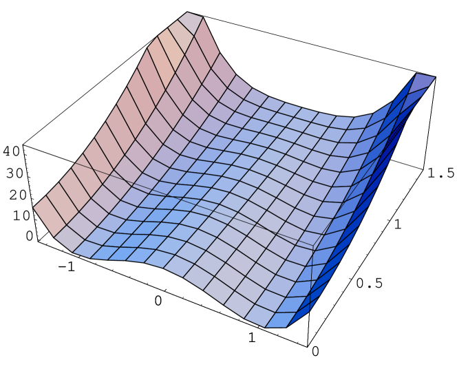
  Figure 3: Typical potential $V(\phi,\psi)$ for hybrid inflation.

  This category of models, which appeared rather recently, relies on the presence of two scalar fields: one plays the traditional rôle of the inflaton, while the other is necessary to end inflation.

  As an illustration, let us consider the original model of hybrid inflation [6] based on the potential

  $$V(\phi,\psi)={1\over 2}m^{2}\phi^{2}+{1\over 2}\lambda^{\prime}\psi^{2}\phi^{2}+{1\over 4}\lambda\left(M^{2}-\psi^{2}\right)^{2}.$$ (73)

  For values of the field $\phi$ larger than the critical value $\phi_{c}=\lambda M^{2}/\lambda^{\prime}$, the potential for $\psi$ has its minimum at $\psi=0$. This is the case during inflation. $\psi$ is thus trapped in this minimum $\psi=0$, so that the effective potential for the scalar field $\phi$, which plays the rôle of the inflaton, is given by

  $$V_{eff}(\phi)=V_{0}+{1\over 2}m^{2}\phi^{2},$$ (74)

  with $V_{0}=\lambda M^{4}/4$. During the inflationary phase, the field $\phi$ slow-rolls until it reaches the critical value $\phi_{c}$. The shape of the potential for $\psi$ is then modified and new minima appear in $\psi=\pm M$. $\psi$ will thus roll down into one of these new minima and, as a consequence, inflation will end.

  As far as inflation is concerned, hybrid inflation scenarios correspond effectively to single-field models with a potential characterized by $V^{\prime\prime}(\phi)>0$ and $0<\epsilon<\eta$. A typical potential is

  $$V(\phi)=\Lambda^{4}\left[1+\left({\phi\over\mu}\right)^{p}\right].$$ (75)

  Once more, this potential can be seen as the lowest order in a Taylor expansion about the origin.

  In the case of hybrid models, the value $\phi_{N}$ of the scalar field as a function of the number of e-folds before the end of inflation is not determined by the above potential and, therefore, $(\phi_{N}/\mu)$ can be considered as a freely adjustable parameter.

Many more details on inflationary models can be found in e.g. [7, 8, 9].

4 The theory of cosmological perturbations

So far, we have concentrated our attention on strictly homogeneous and isotropic aspects of cosmology. Of course, this idealized version, although extremely useful, is not sufficient to account for real cosmology and it is now time to turn to the study of deviations from homogeneity and isotropy.

In cosmology, inhomogeneities grow because of the attractive nature of gravity, which implies that inhomogeneities were much smaller in the past. As a consequence, for most of their evolution, inhomogeneities can be treated as linear perturbations. The linear treatment ceases to be valid on small scales in our recent past, hence the difficulty to reconstruct the primordial inhomogeneities from large-scale structure, but it is quite adequate to describe the fluctuations of the CMB at the time of last scattering. This is the reason why the CMB is currently the best observational probe of primordial inhomogeneities. For more details on the relativistic theory of cosmological perturbations, which will be briefly introduced in this chapter, the reader is invited to read the standard reviews [10] in the literature.

From now on, we will be mostly working with the conformal time $\eta$, instead of the cosmic time $t$. The conformal time is defined as

$$\eta=\int{dt\over a(t)}$$ (76)

so that the (spatially flat) FLRW metric takes the remarkably simple form

$$ds^{2}=a^{2}(\eta)\left[-d\eta^{2}+\delta_{ij}dx^{i}dx^{j}\right].$$ (77)

4.1 Perturbations of the geometry

Let us start with the linear perturbations of the geometry. The most general linear perturbation of the FLRW metric can be expressed as

$$ds^{2}=a^{2}\left\{-(1+2A)d\eta^{2}+2B_{i}dx^{i}d\eta+\left(\delta_{ij}+h_{ij}\right)dx^{i}dx^{j}\right\},$$ (78)

where we have considered only the spatially flat FLRW metric.

We have introduced a time plus space decomposition of the perturbations. The indices $i$, $j$ stand for spatial indices and the perturbed quantities defined in (78) can be seen as three-dimensional tensors, for which the indices can be lowered (or raised) by the spatial metric $\delta_{ij}$ (or its inverse).

It is very convenient to separate the perturbations into three categories, the so-called “scalar”, “vector” and “tensor” modes. For example, a spatial vector field $B^{i}$ can be decomposed uniquely into a longitudinal part and a transverse part,

$$B_{i}=\nabla_{i}B+{\bar{B}}_{i},\quad\nabla_{i}{\bar{B}}^{i}=0,$$ (79)

where the longitudinal part is curl-free and can thus be expressed as a gradient, and the transverse part is divergenceless. One thus gets one “scalar” mode, $B$ , and two “vector” modes ${\bar{B}}^{i}$ (the index $i$ takes three values but the divergenceless condition implies that only two components are independent.

A similar procedure applies to the symmetric tensor $h_{ij}$, which can be decomposed as

$$h_{ij}=2C\delta_{ij}+2\nabla_{i}\nabla_{j}E+2\nabla_{(i}E_{j)}+\overline{E}_{ij},$$ (80)

with $\overline{E}^{ij}$ transverse and traceless (TT), i.e. $\nabla_{i}\overline{E}^{ij}=0$ (transverse) and $\overline{E}^{ij}\delta_{ij}=0$ (traceless), and $E_{i}$ transverse. The parentheses around the indices denote symmetrization, namely $2\nabla_{(i}E_{j)}=\nabla_{i}E_{j}+\nabla_{j}E_{i}$. We have thus defined two scalar modes, $C$ and $E$, two vector modes, $E_{i}$, and two tensor modes, ${\bar{E}}_{ij}$.

In the following, we will be mainly interested in the metric with only scalar perturbations, since scalar modes are the most relevant for cosmology and they can be treated independently of the vector and tensor modes. In matrix notation, the perturbed metric will thus be of the form

$$g_{\mu\nu}=a^{2}\left[\begin{array}[]{ccc}-(1+2A)&&\nabla_{i}B\\ &&\\ \nabla_{j}B&&\left\{(1+2C)\delta_{ij}+2\nabla_{i}\nabla_{j}E\right\}\end{array}\right]\,.$$ (81)

After the description of the perturbed geometry, we turn to the perturbations of the matter in the next subsection.

4.2 Perturbations of the matter

Quite generally, the perturbed energy-momentum tensor can be written in the form

$$T^{\mu}_{\nu}=\left[\begin{array}[]{ccc}-(\rho+\delta\rho)&&q_{j}\\ &&\\ -q^{i}+(\rho+P)B^{i}&&(P+\delta P)\delta^{i}_{j}+\pi^{i}_{j}\end{array}\right]\,,$$ (82)

where $q_{i}$ is the momentum density and $\pi^{i}_{j}$ is the anisotropic stress tensor, which is traceless, i.e. $\pi_{k}^{k}=0$. One can then decompose these tensors into scalar, vector and tensor components, as before for the metric components, so that

$$q_{i}=\nabla_{i}q+\bar{q}_{i},\quad\nabla_{i}\bar{q}^{i}=0,$$ (83)

and

$$\pi_{ij}=\nabla_{i}\nabla_{j}\pi-{1\over 3}\delta_{ij}\nabla_{k}\nabla^{k}\pi+2\nabla_{(i}\pi_{j)}+\bar{\pi}_{ij},\quad\nabla_{k}\pi^{k}=0,\quad\nabla_{k}\bar{\pi}^{kl}=0,\quad\bar{\pi}^{k}_{k}=0.$$ (84)

4.2.1 Fluid

A widely used description for matter in cosmology is that of a fluid. Its homogeneous part is described by the energy-momentum tensor of a perfect fluid, as seen earlier, while its perturbed part can be expressed as

$$\delta T_{0}^{0}= -\delta\rho,$$ (85)

$$\delta T_{0}^{i}= -\left(\rho+p\right)v^{i},\quad\delta T^{0}_{i}=\left(\rho+p\right)\left(v_{i}+B_{i}\right)$$ (86)

$$\delta T^{i}_{j}= \delta P\delta^{i}_{j}+\pi^{i}_{j},$$ (87)

with $\pi_{k}^{k}=0$ as before and where $v^{i}$ is the three-dimensional fluid velocity defined by

$$\delta u^{i}={1\over a}v^{i}.$$ (88)

It is also possible to separate this perturbed energy-momentum tensor into scalar, vector and tensor parts by using decompositions for $v_{i}$ and $\pi_{ij}$ similar to (83) and (84).

4.2.2 Scalar field

Another type of matter, especially useful in the context of inflation, is a scalar field. The homogeneous description has already been given earlier and the perturbed expression for the energy-momentum tensor follows immediately from (41), taking into account the metric perturbations as well. One finds

$$a^{2}\delta T_{0}^{0} = -a^{2}\delta\rho=-\phi^{\prime}{\delta\phi}^{\prime}-a^{2}V^{\prime}\delta\phi+{\phi^{\prime}}^{2}A,$$ (89)

$$a^{2}\delta T^{0}_{i} = a^{2}q_{i}=-\phi^{\prime}\partial_{i}\delta\phi,$$ (90)

$$a^{2}\delta T^{i}_{j} = -\delta^{i}_{j}\left(a^{2}V^{\prime}\delta\phi+{\phi^{\prime}}^{2}A-\phi^{\prime}\delta\phi^{\prime}\right).$$ (91)

The last equation shows that, for a scalar field, there is no anisotropic stress in the energy-momentum tensor.

4.3 Gauge transformations

It is worth noticing that there is a fundamental difference between the perturbations in general relativity and the perturbations in other field theories where the underlying spacetime is fixed. In the latter case, one can define the perturbation of a given field $\phi$ as

$$\delta\phi(p)=\phi(p)-{\bar{\phi}}(p),$$ (92)

where ${\bar{\phi}}$ is the unperturbed field and $p$ is any point of the spacetime.

In the context of general relativity, spacetime is no longer a frozen background but must also be perturbed if matter is perturbed. As a consequence, the above definition does not make sense since the perturbed quantity $\phi$ lives in the perturbed spacetime ${\cal M}$, whereas the unperturbed quantity ${\bar{\phi}}$ lives in another spacetime: the unperturbed spacetime of reference, which we will denote $\bar{\cal M}$. In order to use a definition similar to (92), one must introduce a one-to-one identification, $\iota$, between the points of $\bar{\cal M}$ and those of ${\cal M}$. The perturbation of the field can then be defined as

$$\delta\phi(\bar{p})=\phi(\iota(\bar{p}))-{\bar{\phi}}(\bar{p}),$$ (93)

where $\bar{p}$ is a point of $\bar{\cal M}$.

However, the identification $\iota$ is not uniquely defined, and therefore the definition of the perturbation depends on the particular choice for $\iota$: two different identifications, $\iota_{1}$ and $\iota_{2}$ say, lead to two different definitions for the perturbations. This ambiguity can be related to the freedom of choice of the coordinate system. Indeed, if one is given a coordinate system in $\bar{\cal M}$, one can transport it into ${\cal M}$ via the identification. $\iota_{1}$ and $\iota_{2}$ thus define two different coordinate systems in ${\cal M}$, and in this respect, a change of identification can be seen as a change of coordinates in ${\cal M}$.

The metric perturbations, introduced in (78), are modified in a coordinate transformation of the form

$$x^{\alpha}\rightarrow x^{\alpha}+\xi^{\alpha},\qquad\xi^{\alpha}=(\xi^{0},\xi^{i}).$$ (94)

It can be shown that the change of the metric components can be expressed as

$$\Delta\left(\delta g_{\mu\nu}\right)=-2D_{(\mu}\xi_{\nu)}.$$ (95)

where $\Delta$ represents the variation, due the coordinate transformation, at the same old and new coordinates (and thus at different physical points). The above variation can be decomposed into individual variations for the various components of the metric defined earlier. One finds

$$\Delta A = -{\xi^{0}}^{\prime}-{\cal H}\xi^{0}$$ (96)

$$\Delta B_{i} = \nabla_{i}\xi^{0}-\xi_{i}^{\prime}$$ (97)

$$\Delta h_{ij} = -2\left(\nabla_{(i}\xi_{j)}-{\cal H}\xi^{0}\delta_{ij}\right).$$ (98)

The effect of a coordinate transformation can also be decomposed along the scalar, vector and tensor sectors introduced earlier. The generator $\xi^{\alpha}$ of the coordinate transformation can be written as

$$\xi^{\alpha}=(\xi^{0},\nabla^{i}\xi+\overline{\xi}^{i}),$$ (99)

with $\overline{\xi}^{i}$ transverse. This shows explicitly that $\xi^{\alpha}$ contains two scalar components, $\xi^{0}$ and $\xi$, and two vector components, $\overline{\xi}^{i}$. The transformations (96-98) are then decomposed into :

$$A \rightarrow A-{\xi^{0}}^{\prime}-{\cal H}\xi^{0}$$

$$B \rightarrow B+\xi^{0}-\xi^{\prime}$$

$$C \rightarrow C-{\cal H}\xi^{0}$$

$$E \rightarrow E-\xi$$ (100)

$$\overline{B}^{i} \rightarrow \overline{B}^{i}-{{\overline{\xi}}^{i}}^{\prime}$$

$$E^{i} \rightarrow E^{i}-\overline{\xi}^{i}.$$

The tensor perturbations remain unchanged since $\xi^{\alpha}$ does not contain any tensor component. The matter perturbations, either in the fluid description or in the scalar field description, follow similar transformation laws in a coordinate change.

In order to study the physically relevant modes and not spurious modes due to coordinate ambiguities, two strategies can a priori be envisaged. The first consists in working from the start in a specific gauge. A familiar choice in the literature on cosmological perturbations is the longitudinal gauge (also called conformal Newton gauge), which imposes

$$B_{\rm L}=0,\quad E_{\rm L}=0.$$ (101)

The second approach consists in defining gauge-invariant variables, i.e. variables that are left unchanged under a coordinate transformation. For the scalar metric perturbations, we start with four quantities ($A$, $B$, $C$ and $E$) and we can use two gauge transformations ($\xi^{0}$ and $\xi$). This implies that the scalar metric perturbations must be described by two independent gauge-invariant quantities. Two such quantities are

$$\Phi=A+(B-E^{\prime})^{\prime}+{\cal H}(B-E^{\prime})$$ (102)

and

$$\Psi=-C-{\cal H}(B-E^{\prime}),$$ (103)

as it can be checked by considering the explicit transformations in (100). It turns out that, in the longitudinal gauge, the remaining scalar perturbations $A_{\rm L}$ and $C_{\rm L}$ are numerically equivalent to the gauge-invariant quantities just defined $\Phi$ and $-\Psi$.

In practice, one can combine the two strategies by doing explicit calculations in a given gauge and then by relating the quantities defined in this gauge to some gauge-invariant variables. It is then possible to translate the results in any other gauge. In the rest of these lectures, we will use the longitudinal gauge.

4.4 The perturbed Einstein equations

After having defined the metric and the matter perturbations, we can now relate them via the perturbed Einstein equations. We will consider here explicitly only the scalar sector, which is the most complicated but also the most interesting for cosmological applications.

Starting from the perturbed metric (81), one can compute the components of Einstein’s tensor at linear order. In the longitudinal gauge, i.e. with $B_{\rm L}=E_{\rm L}=0$, one finds

$$\left(\delta G^{0}_{0}\right)_{\rm L} = {2\over a^{2}}\left[3{\cal H}^{2}A_{\rm L}-3{\cal H}C^{\prime}_{\rm L}+\nabla^{2}C_{\rm L}\right]$$ (104)

$$\left(\delta G^{0}_{i}\right)_{\rm L} = {2\over a^{2}}\nabla_{i}\left[-{\cal H}A_{\rm L}+C^{\prime}_{\rm L}\right]$$ (105)

$$\left(\delta G^{i}_{j}\right)_{\rm L} = {1\over a^{2}}\nabla^{i}\nabla_{j}\left(-C_{\rm L}-A_{\rm L}\right)+{1\over a^{2}}\left[-2C_{\rm L}^{\prime\prime}-4{\cal H}C_{\rm L}^{\prime}+\nabla^{2}C_{\rm L}\right.$$ (107)

$$\left.+2{\cal H}A_{\rm L}^{\prime}+\nabla^{2}A_{\rm L}+2\left(2{\cal H}^{\prime}+{\cal H}^{2}\right)A_{\rm L}\right]\delta^{i}_{j}.$$

Combining with the perturbations of the energy-momentum tensor given in (82), the perturbed Einstein equations yield, in the longitudinal gauge, the following relations: the energy constraint (from (104))

$$3{\cal H}^{2}A_{\rm L}-3{\cal H}C_{\rm L}^{\prime}+\nabla^{2}C_{\rm L}=-4\pi Ga^{2}\delta\rho_{\rm L},$$ (108)

the momentum constraint (from (105))

$$C_{\rm L}^{\prime}-{\cal H}A_{\rm L}=4\pi G\,a^{2}\,q_{\rm L},$$ (109)

the “anisotropy constraint” (from the traceless part of (107))

$$-A_{\rm L}-C_{\rm L}=8\pi G\,a^{2}\,\pi_{\rm L},$$ (110)

and finally

$$C_{\rm L}^{\prime\prime}+2{\cal H}C_{\rm L}^{\prime}-{\cal H}A_{\rm L}^{\prime}-(2{\cal H}^{\prime}+{\cal H}^{2})A_{\rm L}-{1\over 3}\nabla^{2}(A_{\rm L}+C_{\rm L})=-4\pi G\,\delta P_{\rm L},$$ (111)

obtained from the trace of (107).

The combination of the energy and momentum constraints gives the useful relation

$$\nabla^{2}\Psi=4\pi Ga^{2}\left(\delta\rho_{\rm L}-3{\cal H}q_{\rm L}\right)\equiv 4\pi Ga^{2}\delta\rho_{c},$$ (112)

where we have introduced the comoving energy density perturbation $\delta\rho_{c}$: this gauge-invariant quantity corresponds, according to its definition, to the energy density perturbation measured in comoving gauges characterized by $\delta T^{0}_{i}=q_{i}=0$. We have also replaced $C_{\rm L}$ by $-\Psi$. Note that the above equation is quite similar to the Newtonian Poisson equation, but with quantities whose natural interpretation is given in different gauges.

4.5 Equations for the matter

As mentioned earlier, a consequence of Einstein’s equations is that the total energy-momentum tensor is covariantly conserved (see Eq. (9)). For a fluid, the conservation of the energy-momentum tensor leads to a continuity equation that generalizes the continuity equation of fluid mechanics, and a momentum conservation equation that generalizes the Euler equation. In the case of a single fluid, combinations of the perturbed Einstein equations obtained in the previous subsection lead necessarily to the perturbed continuity and Euler equations for the fluid. In the case of several non-interacting fluids, however, one must impose separately the covariant conservation of each energy-momentum tensor: this is not a consequence of Einstein’s equations, which impose only the conservation of the total energy-momentum tensor.

In the perspective to deal with several cosmological fluids, it is therefore useful to write the perturbation equations, satisfied by a given fluid, that follow only from the conservation of the corresponding energy-momentum tensor, and independently of Einstein’s equations.

The continuity equation can be obtained by perturbing $u^{\mu}D_{\nu}T^{\nu}_{\mu}=0$. One finds, in any gauge,

$$\delta\rho^{\prime}+3{\cal H}\left(\delta\rho+\delta P\right)+\left(\rho+P\right)\left(3C^{\prime}+\nabla^{2}E^{\prime}+\nabla^{2}v\right)=0.$$ (113)

Dividing by $\rho$, this can be reexpressed in terms of the density contrast $\delta=\delta\rho/\rho$:

$$\delta^{\prime}+3{\cal H}\left({\delta P\over\delta\rho}-w\right)\delta+(1+w)\left(\nabla^{2}v+3C^{\prime}+\nabla^{2}E^{\prime}\right)=0,$$ (114)

where $w=p/\rho$ ($w$ is not necessarily constant here). The perturbed Euler equation is derived from the spatial projection of $\delta(D_{\nu}T^{\nu}_{\mu})=0$. This gives

$$\left(v+B\right)^{\prime}+\left(1-3c_{s}^{2}\right){\cal H}\left(v+B\right)+A+{\delta P\over\rho+P}+{2\over 3(\rho+P)}\nabla^{2}\pi=0,$$ (115)

where $c_{s}$ is the sound speed, which is related to the time derivatives of the background energy density and pressure:

$$c_{s}^{2}={p^{\prime}\over\rho^{\prime}}.$$ (116)

There are as many systems of equations (114-115) as the number of fluids. If the fluids are interacting, one must add an interaction term on the right-hand side of the Euler equations.

Finally, let us stress that the fluid description is not always an adequate approximation for cosmological matter. A typical example is the photons during and after recombination: their mean free path becomes so large that they must be treated as a gas, which requires the use of the Boltzmann equation (see e.g. [11] for a presentation of the Boltzmann equation in the cosmological context).

4.6 Initial conditions for standard cosmology

The notion of initial conditions depends in general on the context, since the initial conditions for a given period in the history of the universe can be seen as the final conditions of the previous phase. In cosmology, “initial conditions” usually refer to the state of the perturbations during the radiation dominated era (of standard cosmology) and on wavelengths larger than the Hubble radius.

Let us first address in details the question of initial conditions in the simple case of a single perfect fluid, radiation, with equation of state $p=\rho/3$ (which gives $c_{s}^{2}=w=1/3$). The four key equations are the continuity, Euler, Poisson and anisotropy equations, respectively Eqs (114), (115), (112) and (110). In terms of the Fourier components,

$$Q({\vec{k}})=\int{d^{3}x\over(2\pi)^{3/2}}e^{-i{\vec{k}}.{\vec{x}}}Q({\vec{x}}),$$ (117)

and of the dimensionless quantity

$$x\equiv k\eta$$ (118)

(during the radiation dominated era ${\cal H}=1/\eta$), the four equations can be rewritten as

$${d\delta\over dx}-{4\over 3}{\cal V}+4{dC\over dx}=0,$$ (119)

$${d{\cal V}\over dx}+{1\over 4}\delta+A=0,$$ (120)

$$x^{2}C={3\over 2}\left(\delta-{4\over x}{\cal V}\right)$$ (121)

$$C=-A.$$ (122)

We have introduced the quantity ${\cal V}\equiv kv$, which has the dimension of a velocity. Since we are interested in perturbations with wavelength larger than the Hubble radius, i.e. such that $x=k/{\cal H}\ll 1$, it is useful to consider a Taylor expansion for the various perturbations, for instance

$${\cal V}={\cal V}^{(0)}+x{\cal V}^{(1)}+{x^{2}\over 2}{\cal V}^{(2)}+\dots$$ (123)

One then substitutes these Taylor expansions into the above system of equations. In particular, the Poisson equation (121) gives

$${\cal V}^{(0)}=0,$$ (124)

in order to avoid a divergence, as well as

$${\cal V}^{(1)}={1\over 4}\delta^{(0)}.$$ (125)

The Euler equation (120) then gives

$$A^{(0)}=-{1\over 2}\delta^{(0)}.$$ (126)

The conclusion is that the initial conditions for each Fourier mode are determined by a single quantity, e.g. $\delta^{(0)}$, the other quantities being related via the above constraints.

In general, one must consider several cosmological fluids. Typically, the “initial” or “primordial” perturbations are defined deep in the radiation era but at temperatures low enough, i.e. after nucleosynthesis, so that the main cosmological components reduce to the usual photons, baryons, neutrinos and cold dark matter (CDM). The system (119-122) must thus be generalized to include a continuity equation and a Euler equation for each fluid. The above various cosmological species can be characterized by their number density, $n_{X}$, and their energy density $\rho_{X}$. In a multi-fluid system, it is useful to distinguish adiabatic and isocurvature perturbations.

The adiabatic mode is defined as a perturbation affecting all the cosmological species such that the relative ratios in the number densities remain unperturbed, i.e. such that

$$\delta\left(n_{X}/n_{Y}\right)=0.$$ (127)

It is associated with a curvature perturbation, via Einstein’s equations, since there is a global perturbation of the matter content. This is why the adiabatic perturbation is also called curvature perturbation. In terms of the energy density contrasts, the adiabatic perturbation is characterized by the relations

$${1\over 4}\delta_{\gamma}={1\over 4}\delta_{\nu}={1\over 3}\delta_{b}={1\over 3}\delta_{c},$$ (128)

They follow directly from the prescription (127), each coefficient depending on the equation of state of the particuler species.

Since there are several cosmological species, it is also possible to perturb the matter components without perturbing the geometry. This corresponds to isocurvature perturbations, characterized by variations in the particle number ratios but with vanishing curvature perturbation. The variation in the relative particle number densities between two species can be quantified by the so-called entropy perturbation

$$S_{A,B}\equiv{{\delta}n_{A}\over n_{A}}-{{\delta}n_{B}\over n_{B}}.$$ (129)

When the equation of state for a given species is such that $w\equiv p/\rho={\rm Const}$, then one can reexpress the entropy perturbation in terms of the density contrast, in the form

$$S_{A,B}\equiv{\delta_{A}\over 1+w_{A}}-{\delta_{B}\over 1+w_{B}}.$$ (130)

It is convenient to choose a species of reference, for instance the photons, and to define the entropy perturbations of the other species relative to it:

$$S_{b} \equiv\delta_{b}-{3\over 4}\delta_{\gamma},$$ (131)

$$S_{c} \equiv\delta_{c}-{3\over 4}\delta_{\gamma},$$ (132)

$$S_{\nu} \equiv{3\over 4}\delta_{\nu}-{3\over 4}\delta_{\gamma},$$ (133)

thus define respectively the baryon isocurvature mode, the CDM isocurvature mode, the neutrino isocurvature mode. In terms of the entropy perturbations, the adiabatic mode is obviously characterized by $S_{b}=S_{c}=S_{\nu}=0$.

In summary, we can decompose a general perturbation, described by four density contrasts, into one adiabatic mode and three isocurvature mode. In fact, the problem is slightly more complicated because the evolution of the initial velocity fields. For a single fluid, we have seen that the velocity field is not an independent initial condition but depends on the density contrast so that there is no divergence backwards in time. In the case of the four species mentioned above, there remains however one arbitrary relative velocity between the species, which gives an additional mode, usually named the neutrino isocurvature velocity perturbation.

The CMB is a powerful way to study isocurvature perturbations because (primordial) adiabatic and isocurvature perturbations produce very distinctive features in the CMB anisotropies [12]. Whereas an adiabatic initial perturbation generates a cosine oscillatory mode in the photon-baryon fluid, leading to an acoustic peak at $\ell\simeq 220$ (for a flat universe), a pure isocurvature initial perturbation generates a sine oscillatory mode resulting in a first peak at $\ell\simeq 330$. The unambiguous observation of the first peak at $\ell\simeq 220$ has eliminated the possibility of a dominant isocurvature perturbation. The recent observation by WMAP of the CMB polarization has also confirmed that the initial perturbation is mainly an adiabatic mode. But this does not exclude the presence of a subdominant isocurvature contribution, which could be detected in future high-precision experiments such as Planck.

4.7 Super-Hubble evolution

In the case of adiabatic perturbations, there is only one (scalar) dynamical degree of freedom. One can thus choose either an energy density perturbation or a metric perturbation, to study the dynamics, the other quantities being determined by the constraints.

If one considers the metric perturbation $\Psi=\Phi$ (assuming $\pi=0$), one can combine Einstein’s equations (111), with $\delta p=c_{s}^{2}\delta\rho$ (for adiabatic perturbations), and (108) to obtain a second-order differential equation in terms of $\Psi$ only:

$$\Psi^{\prime\prime}+3{\cal H}(1+c_{s}^{2})\Psi^{\prime}+\left[2{\cal H}^{\prime}+(1+3c_{s}^{2}){\cal H}\right]\Psi-k^{2}c_{s}^{2}\Psi=0.$$ (134)

Using the background Friedmann equations, the sound speed can be reexpressed in terms of the scale factor and its derivatives. For scales larger than the sonic horizon, i.e. such that $kc_{s}\ll{\cal H}$, the above equation can be integrated explicitly and yields

$$\Psi={{\cal H}\over a^{2}}\left[\alpha\int d\eta{a^{2}\left({\cal H}^{\prime}-{\cal H}^{2}\right)\over{\cal H}^{2}}+\beta\right],$$ (135)

where $\alpha$ and $\beta$ are two integration constants.

For a scale factor evolving like $a\propto t^{p}$, one gets

$$\Psi=-{\alpha\over p+1}+\beta\,p\,t^{-p-1}.$$ (136)

They are two modes: a constant mode and a decaying mode. Note that, in the previous subsection on the initial conditions, we eliminated the decaying mode to avoid the divergence when going backwards in time.

In a transition between two cosmological phases characterized respectively by the scale factors $a\propto t^{p_{1}}$ and $a\propto t^{p_{2}}$, one can easily finds the relation between the asymptotic behaviours of $\Psi$ (i.e. after the decaying mode becomes negligible) by using the constancy of $\alpha$. This gives

$$\Psi_{2}={p_{2}+1\over p_{1}+1}\Psi_{1}.$$ (137)

This is valid only asymptotically. In the case of a sharp transition, $\Psi$ must be continuous at the transition and the above relation will apply only after some relaxation time. For a transition radiation/non-relativistic matter, one finds

$$\Psi_{mat}={9\over 10}\Psi_{rad}.$$ (138)

In practice and for more general cases, it turns out that it is much more convenient to follow the evolution of cosmological perturbations by resorting to quantities that are conserved on super-Hubble scales. A familiar example of such a quantity is the curvature perturbation on uniform-energy-density hypersurfaces, which can be expressed in any gauge as

$$\zeta=C-{\cal H}{\delta\rho\over\rho^{\prime}}.$$ (139)

This is a gauge-invariant quantity by definition. The conservation equation (114) can then be rewritten as

$$\zeta^{\prime}=-{{\cal H}\over\rho+P}\delta P_{nad}-{1\over 3}\nabla^{2}(E^{\prime}+v),$$ (140)

where $\delta P_{nad}$ is the non-adiabatic part of the pressure perturbation, defined by

$$\delta P_{nad}=\delta P-c_{s}^{2}\delta\rho.$$ (141)

The expression (140) shows that $\zeta$ is conserved on super-Hubble scales in the case of adiabatic perturbations.

Another convenient quantity, which is sometimes used in the literature instead of $\zeta$, is the curvature perturbation on comoving hypersurfaces, which can be written in any gauge as

$$-{\cal R}=C+{{\cal H}\over\rho+P}q.$$ (142)

It is easy to relate the two quantities $\zeta$ and ${\cal R}$. Substituting e.g. $\delta\rho=\delta\rho_{c}+3{\cal H}q$, which follows from the definition (see (112)) of the comoving energy density perturbation, into (139), one finds

$$\zeta=-{\cal R}+{\delta\rho_{c}\over\rho+P}.$$ (143)

Using Einstein’s equations, in particular (112), this can be rewritten as

$$\zeta=-{\cal R}-{2\rho\over 3(\rho+P)}\left({k\over aH}\right)^{2}\Psi.$$ (144)

The latter expression shows that $\zeta$ and ${\cal R}$ coincide in the super-Hubble limit $k\ll aH$.

The quantity ${\cal R}$ can also be expressed in terms of the two Bardeen potentials $\Phi$ and $\Psi$. Using the momentum constraint (109) and the Friedmann equations, one finds

$${\cal R}=\Psi-{H\over\dot{H}}\left(\dot{\Psi}+H\Phi\right).$$ (145)

In a cosmological phase dominated by a fluid with no anisotropic stress, so that $\Phi=\Psi$, and with an equation of state $P=w\rho$ with $w$ constant, we have already seen that $\Psi$ is constant with time. Since the scale factor evolves like $a\propto t^{p}$ with $p=2/3(1+w)$, the relation (145) between ${\cal R}$ and $\Psi$ reduces to

$${\cal R}={5+3w\over 3(1+w)}\Psi.$$ (146)

In the radiation era, ${\cal R}=(3/2)\Psi$, whereas in the matter era, ${\cal R}=(5/3)\Psi$, and since ${\cal R}$ is conserved, one recovers the conclusion given in Eq. (138).

During inflation, $w\simeq-1$ and

$$w+1={\dot{\phi}^{2}\over\rho}\simeq-{2\over 3}{\dot{H}\over H^{2}}$$ (147)

so that

$${\cal R}\simeq-{H^{2}\over\dot{H}}\Psi_{inf}.$$ (148)

For a scalar field, the perturbed equation of motion reads

$$\ddot{\delta\sigma}+3H\dot{\delta\sigma}+\left({k^{2}\over a^{2}}+V^{\prime\prime}\right)\delta\sigma=\dot{\sigma}\left(\dot{\Phi}+3\dot{\Psi}\right)-2V^{\prime}\Phi.$$ (149)

5 Quantum fluctuations and “birth” of cosmological perturbations

In the previous section, we have discussed the classical evolution of the cosmological perturbations. In the classical context, the initial conditions, defined deep in the radiation era, are a priori arbitrary. What is remarkable with inflation is that the accelerated expansion can convert initial vacuum quantum fluctuations into “macroscopic” cosmological perturbations (see [13] for the seminal works). In this sense, inflation provides us with “natural” initial conditions, which turn out to be the initial conditions that agree with the present observations.

5.1 Massless scalar field in de Sitter

As a warming-up, it is instructive to discuss the case of a massless scalar field in a so-called de Sitter universe, or a FLRW spacetime with exponential expansion, $a\propto\exp(Ht)$. In conformal time, the scale factor is given by

$$a(\eta)=-{1\over H\eta}.$$ (150)

The conformal time is here negative (so that the scale factor is positive) and goes from $-\infty$ to $0$. The action for a massless scalar field in this geometry is given by

$$S=\int d^{4}x\sqrt{-g}\left(-{1\over 2}\partial_{\mu}\phi\partial^{\mu}\phi\right)=\int d\eta\,\,d^{3}x\,\,a^{4}\left[{1\over 2a^{2}}{\phi^{\prime}}^{2}-{1\over 2a^{2}}{\vec{\nabla}\phi}^{2}\right],$$ (151)

where we have substituted in the action the cosmological metric (77). Note that, whereas we still allow for spatial variations of the scalar field, i.e. inhomogeneities, we will assume here, somewhat inconsistently, that the geometry is completely fixed as homogeneous. We will deal later with the question of the metric perturbations.

It is possible to write the above action with a canonical kinetic term via the change of variable

$$u=a\phi.$$ (152)

After an integration by parts, the action (151) can be rewritten as

$$S={1\over 2}\int d\eta\,\,d^{3}x\,\left[{u^{\prime}}^{2}-{\vec{\nabla}u}^{2}+{a^{\prime\prime}\over a}u^{2}\right].$$ (153)

The first two terms are familiar since they are the same as in the action for a free massless scalar field in Minkowski spacetime. The fact that our scalar field here lives in de Sitter spacetime rather than Minkowski has been reexpressed as a time-dependent effective mass

$$m^{2}_{eff}=-{a^{\prime\prime}\over a}=-{2\over\eta^{2}}.$$ (154)

Our next step will be to quantize the scalar field $u$ by using the standard procedure of quantum field theory. One first turns $u$ into a quantum field denoted $\hat{u}$, which we expand in Fourier space as

$$\hat{u}(\eta,\vec{x})={1\over(2\pi)^{3/2}}\int d^{3}k\left\{{\hat{a}}_{\vec{k}}u_{k}(\eta)e^{i\vec{k}.\vec{x}}+{\hat{a}}_{\vec{k}}^{\dagger}u_{k}^{*}(\eta)e^{-i\vec{k}.\vec{x}}\right\},$$ (155)

where the $\hat{a}^{\dagger}$ and $\hat{a}$ are creation and annihilation operators, which satisfy the usual commutation rules

$$\left[{\hat{a}}_{\vec{k}},{\hat{a}}_{\vec{k}^{\prime}}\right]=\left[{\hat{a}^{\dagger}}_{\vec{k}},{\hat{a}^{\dagger}}_{\vec{k}^{\prime}}\right]=0,\quad\left[{\hat{a}}_{\vec{k}},{\hat{a}^{\dagger}}_{\vec{k}^{\prime}}\right]=\delta(\vec{k}-\vec{k}^{\prime}).$$ (156)

The function $u_{k}(\eta)$ is a complex time-dependent function that must satisfy the classical equation of motion in Fourier space, namely

$$u_{k}^{\prime\prime}+\left(k^{2}-{a^{\prime\prime}\over a}\right)u_{k}=0,$$ (157)

which is simply the equation of motion for an oscillator with a time-dependent mass. In the case of a massless scalar field in Minkowski spacetime, this effective mass is zero ($a^{\prime\prime}/a=0$) and one usually takes $u_{k}=(\hbar/2k)^{1/2}e^{-ik\eta}$ (the choice for the normalization factor will be clear below). In the case of de Sitter, one can solve explicitly the above equation with $a^{\prime\prime}/a=2/\eta^{2}$ and the general solution is given by

$$u_{k}=\alpha e^{-ik\eta}\left(1-{i\over k\eta}\right)+\beta e^{ik\eta}\left(1+{i\over k\eta}\right).$$ (158)

Canonical quantization consists in imposing the following commutation rules on the $\eta=$constant hypersurfaces:

$$\left[\hat{u}(\eta,\vec{x}),\hat{u}(\eta,\vec{x}^{\prime})\right]=\left[\hat{\pi}_{u}(\eta,\vec{x}),\hat{\pi}_{u}(\eta,\vec{x}^{\prime})\right]=0$$ (159)

and

$$\left[\hat{u}(\eta,\vec{x}),\hat{\pi}_{u}(\eta,\vec{x}^{\prime})\right]=i\hbar\delta(\vec{x}-\vec{x}^{\prime}),$$ (160)

where $\pi_{u}\equiv\delta S/\delta u^{\prime}$ is the conjugate momentum of $u$. In the present case, $\pi_{u}=u^{\prime}$ since the kinetic term is canonical.

Subtituting the expansion (155) in the commutator (160), and using the commutation rules for the creation and annihilation operators (156), one obtains the relation

$$u_{k}{u^{\prime}_{k}}^{*}-u_{k}^{*}u^{\prime}_{k}=i\hbar,$$ (161)

which determines the normalization of the Wronskian.

The choice of a specific function $u_{k}(\eta)$ corresponds to a particular prescription for the physical vacuum $|0\rangle$, defined by

$${\hat{a}}_{\vec{k}}|0\rangle=0.$$ (162)

A different choice for $u_{k}(\eta)$ is associated to a different decomposition into creation and annihilitation modes and thus to a different vacuum.

Let us now note that the wavelength associated with a given mode $k$ can always be found within the Hubble radius provided one goes sufficiently far backwards in time, since the comoving Hubble radius is shrinking during inflation. In other words, for $|\eta|$ sufficiently big, one gets $k|\eta|\gg 1$. Moreover, for a wavelength smaller than the Hubble radius, one can neglect the influence of the curvature of spacetime and the mode behaves as in a Minkowski spacetime, as can also be checked explicitly with the equation of motion (157) (the effective mass is negligible for $k|\eta|\gg 1$). Therefore, the most natural physical prescription is to take the particular solution that corresponds to the usual Minkowski vacuum, i.e. $u_{k}\sim\exp(-ik\eta)$, in the limit $k|\eta|\gg 1$. In view of (158), this corresponds to the choice

$$u_{k}=\sqrt{\hbar\over 2k}e^{-ik\eta}\left(1-{i\over k\eta}\right),$$ (163)

where the coefficient has been determined by the normalisation condition (161). This choice, in the jargon of quantum field theory on curved spacetimes, corresponds to the Bunch-Davies vacuum.

Finally, one can compute the correlation function for the scalar field $\phi$ in the vacuum state defined above. When Fourier transformed, the correlation function defines the power spectrum ${\cal P}_{\phi}(k)$:

$$\langle 0|\hat{\phi}(\vec{x}_{1})\hat{\phi}(\vec{x}_{2})|0\rangle=\int d^{3}k\,\,e^{i\vec{k}.(\vec{x}_{1}-\vec{x}_{2})}{{\cal P}_{\phi}(k)\over 4\pi k^{3}}.$$ (164)

Note that the homogeneity and isotropy of the quantum field is used implicitly in the definition of the power spectrum, which is “diagonal” in Fourier space (homogeneity) and depends only on the norm of $\vec{k}$ (isotropy). In our case, we find

$$2\pi^{2}k^{-3}{\cal P}_{\phi}={|u_{k}|^{2}\over a^{2}},$$ (165)

which gives in the limit when the wavelength is larger than the Hubble radius, i.e. $k|\eta|\ll 1$,

$${\cal P}_{\phi}(k)\simeq\hbar\left({H\over 2\pi}\right)^{2}\qquad(k\ll aH)$$ (166)

Note that, in the opposite limit, i.e. for wavelengths smaller than the Hubble radius ($k|\eta|\gg 1$), one recovers the usual result for fluctuations in Minkowski vacuum, ${\cal P}_{\phi}(k)=\hbar(k/2\pi a)^{2}$.

We have used a quantum description of the scalar field. But the cosmological perturbations are usually described by classical random fields. Roughly speaking, the transition between the quantum and classical (although stochastic) descriptions makes sense when the perturbations exit the Hubble radius. Indeed each of the terms in the Wronskian (161) is roughly of the order $\hbar/2(k\eta)^{3}$ in the super-Hubble limit and the non-commutativity can then be neglected. In this sense, one can see the exit outside the Hubble radius as a quantum-classical transition, although much refinement would be needed to make this statement more precise.

5.2 Quantum fluctuations with metric perturbations

Let us now move to the more realistic case of a perturbed inflaton field living in a perturbed cosmological geometry. The situation is more complicated than in the previous problem, because Einstein’s equations imply that scalar field fluctuations must necessarily coexist with metric fluctuations. A correct treatment, either classical or quantum, must thus involve both the scalar field perturbations and metric perturbations.

In order to quantize this coupled system, the easiest procedure consists in identifying the true degrees of freedom, the other variables being then derived from them via constraint equations. As we saw in the classical analysis of cosmological perturbations, there exists only one scalar degree of freedom in the case of a single scalar field, which we must now identify.

The starting point is the action of the coupled system scalar field plus gravity expanded up to second order in the linear perturbations. Formally this can be written as

$$S[\bar{\phi}+\delta\phi,g_{\mu\nu}=\bar{g}_{\mu\nu}+h_{\mu\nu}]=S^{(0)}[\bar{\phi},\bar{g}_{\mu\nu}]+S^{(1)}[\delta\phi,h_{\mu\nu};\bar{\phi},\bar{g}_{\mu\nu}]+S^{(2)}[\delta\phi,h_{\mu\nu};\bar{\phi},\bar{g}_{\mu\nu}],$$ (167)

where the first term $S^{(0)}$ contains only the homogeneous part, $S^{(1)}$ contains all terms linear in the perturbations (with coefficients depending on the homogeneous variables), and finally $S^{(2)}$ contains the terms quadratic in the linear perturbations. When one substitutes the FLRW equations of motion in $S^{(1)}$ (after integration by parts), one finds that $S^{(1)}$ vanishes, which is not very surprising since this is how one gets the homogeneous equations of motion, via the Euler-Lagrange equations, from the variation of the action.

The term $S^{(2)}$ is the piece we are interested in: the corresponding Euler-Lagrange equations give the equations of motion for the linear perturbations, which we have already obtained; but more importantly, this term enables us to quantize the linear perturbations and to find the correct normalization.

If one restricts oneself to the scalar sector, the quadratic part of the action depends on the four metric perturbations $A$, $B$, $C$, $E$, as well as on the scalar field perturbation $\delta\phi$. After some cumbersome manipulations, by using the FLRW equations of motion, one can show that the second-order action for scalar perturbations can be rewritten in terms of a single variable [14]

$$v=a\left(\delta\phi-{\phi^{\prime}\over{\cal H}}C\right),$$ (168)

which is a linear combination mixing scalar field and metric perturbations. The variable $v$ represents the true dynamical degree of freedom of the system, and one can check immediately that it is indeed a gauge-invariant variable.

In fact, $v$ is proportional to the comoving curvature perturbation defined in (142) and which, in the case of a single scalar field, takes the form

$${\cal R}=-C+{{\cal H}\over\phi^{\prime}}\delta\phi.$$ (169)

Note also that, if one can check a posteriori that $v$ is the variable describing the true degree of freedom by expressing the action in terms of $v$ only (modulo, of course, a multiplicative factor depending only on homogeneous quantities: the $v$ defined here is such that it gives a canonical kinetic term in the action), one can identify $v$ in a systematic way by resorting to Hamiltonian techniques, in particular the Hamilton-Jacobi equation [15].

With the variable $v$, the quadratic action takes the extremely simple form

$$S_{v}={1\over 2}\int d\eta\,\,d^{3}x\,\left[{v^{\prime}}^{2}+\partial_{i}v\partial^{i}v+{z^{\prime\prime}\over z}v^{2}\right],$$ (170)

with

$$z=a{\phi^{\prime}\over{\cal H}}.$$ (171)

This action is thus analogous to that of a scalar field in Minkowski spacetime with a time-dependent mass. One is thus back in a situation similar to the previous subsection, with the notable difference that the effective time-dependent mass is now $z^{\prime\prime}/z$, instead of $a^{\prime\prime}/a$.

The quantity we will be eventually interested in is the comoving curvature perturbation ${\cal R}$, which is related to the canonical variable $v$ by the relation

$$v=-z{\cal R}.$$ (172)

Since, by analogy with (165), the power spectrum for $v$ is given by

$$2\pi^{2}k^{-3}{\cal P}_{v}(k)=|v_{k}|^{2},$$ (173)

the corresponding power spectrum for ${\cal R}$ is found to be

$$2\pi^{2}k^{-3}{\cal P}_{\cal R}(k)={|v_{k}|^{2}\over z^{2}}.$$ (174)

In the case of an inflationary phase in the slow-roll approximation, the evolution of $\phi$ and of $H$ is much slower than that of the scale factor $a$. Consequently, one gets approximately

$${z^{\prime\prime}\over z}\simeq{a^{\prime\prime}\over a},\qquad{\rm(slow-roll)}$$ (175)

and all results of the previous section obtained for $u$ apply directly to our variable $v$ in the slow-roll approximation. This implies that the properly normalized function corresponding to the Bunch-Davies vacuum is approximately given by

$$v_{k}\simeq\sqrt{\hbar\over 2k}e^{-ik\eta}\left(1-{i\over k\eta}\right).$$ (176)

In the super-Hubble limit $k|\eta|\ll 1$ the function $v_{k}$ behaves like

$$v_{k}\simeq-\sqrt{\hbar\over 2k}\,{i\over k\eta}\simeq i\sqrt{\hbar\over 2k}\,{aH\over k},$$ (177)

where we have used $a\simeq-1/(H\eta)$. Consequently, on scales larger than the Hubble radius, the power spectrum for ${\cal R}$ is found, combining (174), (171) and (176), to be given by

$${\cal P}_{\cal R}\simeq{\hbar\over 4\pi^{2}}\left({H^{4}\over\dot{\phi}^{2}}\right)_{k=aH},$$ (178)

where we have reintroduced the cosmic time instead of the conformal time. This is the famous result for the spectrum of scalar cosmological perturbations generated from vacuum fluctuations during a slow-roll inflation phase. Note that during slow-roll inflation, the Hubble parameter and the scalar field velocity slowly evolve: for a given scale, the above amplitude of the perturbations is determined by the value of $H$ and $\dot{\phi}$ when the scale exited the Hubble radius. Because of this effect, the obtained spectrum is not strictly scale-invariant.

It is also instructive to recover the above result by a more intuitive derivation. One can think of the metric perturbations in the radiation era as resulting from the time difference for the end of inflation at different spatial points (separated by distances larger than the Hubble radius), the shift for the end of inflation being a consequence of the scalar field fluctuations $\delta\phi\sim H/2\pi$. Indeed,

$$\Psi_{\rm rad}\sim{\delta a\over a}\sim H\delta t,$$ (179)

and the time shift is related to the scalar field fluctuations by $\delta t\sim\delta\phi/\dot{\phi}$, which implies

$$\Psi_{\rm rad}\sim{H^{2}\over\dot{\phi}},$$ (180)

which agrees with the above result since during the radiation era ${\cal R}=(3/2)\Psi$ (see Eq. (146)). It is also worth noticing that, during inflation, in the case of the slow-roll approximation, the term involving $C$ in the linear combination (168) defining $v$ is negligible with respect to the term involving $\delta\phi$. One can therefore “ignore” the rôle of the metric perturbations during inflation in the computation of the quantum fluctuations and consider only the scalar field perturbations. But this simplification is valid only in the context of slow-roll approximation. It is not valid in the general case, as can be verified for inflation with a power-law scale factor.

5.3 Gravitational waves

We have focused so far our attention on scalar perturbations, which are the most important in cosmology. Tensor perturbations, or primordial gravitational waves, if ever detected in the future, would be a remarkable probe of the early universe. In the inflationary scenario, like scalar perturbations, primordial gravitational waves are generated from vacuum quantum fluctuations. Let us now explain briefly this mechanism.

The action expanded at second order in the perturbations contains a tensor part, which given by

$$S^{(2)}_{g}={1\over 64\pi G}\int d\eta\,d^{3}x\,a^{2}\eta^{\mu\nu}\partial_{\mu}\bar{E}^{i}_{j}\partial_{\nu}\bar{E}^{j}_{i},$$ (181)

where $\eta^{\mu\nu}$ denotes the Minkoswki metric. Apart from the tensorial nature of $E^{i}_{j}$, this action is quite similar to that of a scalar field in a FLRW universe (151), up to a renormalization factor $1/\sqrt{32\pi G}$. The decomposition

$$a\bar{E}^{i}_{j}=\sum_{\lambda=+,\times}\int{d^{3}k\over(2\pi)^{3/2}}v_{k,\lambda}(\eta)\epsilon^{i}_{j}({\vec{k}};\lambda)e^{i\vec{k}.\vec{x}}$$ (182)

where the $\epsilon^{i}_{j}({\vec{k}};\lambda)$ are the polarization tensors, shows that the gravitational waves are essentially equivalent to two massless scalar fields (for each polarization) $\phi_{\lambda}=m_{P}\bar{E}_{\lambda}/2$.

The total power spectrum is thus immediately deduced from (165):

$${\cal P}_{g}=2\times{4\over m_{P}^{2}}\times\hbar\left({H\over 2\pi}\right)^{2},$$ (183)

where the first factor comes from the two polarizations, the second from the renormalization with respect to a canonical scalar field, the last term being the power spectrum for a scalar field derived earlier. In summary, the tensor power spectrum is

$${\cal P}_{g}={2\hbar\over\pi^{2}}\left({H\over m_{P}}\right)_{k=aH}^{2},$$ (184)

where the label recalls that the Hubble parameter, which can be slowly evolving during inflation, must be evaluated when the relevant scale exited the Hubble radius during inflation.

5.4 Power spectra

Let us rewrite the scalar and tensor power spectra, respectively given in (178) and (184), in terms of the scalar field potential only. This can be done by using the slow-roll equations (49-50). One finds for the scalar spectrum

$${\cal P}_{\cal R}={1\over 12\pi^{2}}\left({V^{3}\over m_{P}^{6}{V^{\prime}}^{2}}\right)_{k=aH}$$ (185)

with subscript meaning that the term on the right hand side must be evaluated at Hubble radius exit for the scale of interest. The scalar spectrum can also be written in terms of the first slow-roll parameter defined in (52), in which case it reads

$${\cal P}_{\cal R}={1\over 24\pi^{2}}\left({V\over m_{P}^{4}\epsilon_{V}}\right)_{k=aH}.$$ (186)

From the observations of the CMB fluctuations,

$${\cal P}_{\cal R}^{1/2}={1\over 2\sqrt{6}\pi}\left({V^{1/2}\over m_{P}^{2}\epsilon_{V}^{1/2}}\right)\simeq 5\times 10^{-5}.$$ (187)

If $\epsilon_{V}$ is order $1$, as in chaotic models, one can evaluate the typical energy scale during inflation as

$$V^{1/4}\sim 10^{-3}m_{P}\sim 10^{15}{\rm GeV}.$$ (188)

The tensor power spectrum, in terms of the scalar field potential, is given by

$${\cal P}_{g}={2\over 3\pi^{2}}\left({V\over m_{P}^{4}}\right)_{k=aH}.$$ (189)

The ratio of the tensor and scalar amplitudes is proportional to the slow-roll parameter $\epsilon_{V}$:

$$r\equiv{{\cal P}_{g}\over{\cal P}_{\cal R}}=16\epsilon_{V}.$$ (190)

The scalar and tensor spectra are almost scale invariant but not quite since the scalar field evolves slowly during the inflationary phase. In order to evaluate quantitatively this variation, it is convenient to introduce a scalar spectral index as well as a tensor one, defined respectively by

$$n_{S}(k)-1={d\ln{\cal P}_{\cal R}(k)\over d\ln k},\quad n_{T}(k)={d\ln{\cal P}_{g}(k)\over d\ln k}.$$ (191)

One can express the spectral indices in terms of the slow-roll parameters. For this purpose, let us note that, in the slow-roll approximation, $d\ln k=d\ln(aH)\simeq d\ln a$, so that

$${d\phi\over d\ln a}={\dot{\phi}\over H}\simeq-{V^{\prime}\over 3H^{2}}\simeq-m_{P}^{2}{V^{\prime}\over V},$$ (192)

where the slow-roll equations (49-50) have been used. Therefore, one gets

$$n_{s}(k)-1=2\eta_{V}-6\epsilon_{V},$$ (193)

where $\epsilon_{V}$ and $\eta_{V}$ are the two slow-roll parameters defined in (52) and (54). Similarly, one finds for the tensor spectral index

$$n_{T}(k)=-2\epsilon_{V}.$$ (194)

Comparing with Eq. (190), this yields the relation

$$r=-8n_{T},$$ (195)

the so-called consistency relation which relates purely observable quantities. This means that if one was able to observe the primordial gravitational waves and measure the amplitude and spectral index of their spectrum, a rather formidable task, then one would be able to test directly the paradigm of single field slow-roll inflation.

Finally, let us mention the possibility to get information on inflation from the measurement of the running of the spectral index. Introducing the second-order slow-roll parameter

$$\xi_{V}=m_{P}^{4}\frac{V^{\prime}V^{\prime\prime\prime}}{V^{2}},$$ (196)

the running is given by

$$\frac{dn_{s}}{d\ln k}=-24\epsilon_{V}^{2}+16\epsilon_{V}\eta_{V}-2\xi_{V}.$$ (197)

As one can see, the amplitude of the variation depends on the slow-roll parameters and thus on the models of inflation.

5.5 Conclusions

To conclude, let us mention the existence of more sophisticated models of inflation, such as models where several scalar fields contribute to inflation. In contrast with the single inflaton case, which can generate only adiabatic primordial fluctuations, because all types of matter are decay product of the same inflaton, multi-inflaton models can generate both adiabatic and isocurvature perturbations, which can even be correlated [16].

Another recent direction of research is the possibility to disconnect the fluctuations of the inflaton, the field that drives inflation, from the observed cosmological perturbations, which could have been generated from the quantum fluctuations of another scalar field [17].

From the theoretical point of view an important challenge remains to identify viable and natural candidates for the inflaton field(s) in the framework of high energy physics, with the hope that future observations of the cosmological perturbations will be precise enough to discriminate between various candidates and thus give us a clue about which physics really drove inflation.

Alternative scenarios to inflation can also been envisaged, as long as they can predict unambiguously primordial fluctuations compatible with the present observations. In this respect, one must emphasize that the cosmological perturbations represent today essentially the only observational window that gives access to the very high energy physics, hence the importance for any early universe model to be able to give firm predictions for the primordial fluctuations it generates.

Acknowledgements:

I would like to thank the organizers of this Cargese school for inviting me to lecture at this very nice village in Corsica. I also wish to thank the other lecturers and participants for their remarks and questions, as well as Gérard Smadja and Filippo Vernizzi for their careful reading of the draft.

References

- [1] R. Wald, General Relativity (Chicago, 1984); S.M. Carroll, Spacetime and Geometry, (Addison Wesley, San Francisco, 2004).
- [2] A. H. Guth, Phys. Rev. D 23, 347 (1981).
- [3] A. A. Starobinsky, Phys. Lett. B 91, 99 (1980).
- [4] A. D. Linde, Phys. Lett. B 108, 389 (1982); A. Albrecht and P. J. Steinhardt, Phys. Rev. Lett. 48, 1220 (1982).
- [5] A. D. Linde, Phys. Lett. B 129, 177 (1983).
- [6] A. D. Linde, Phys. Rev. D 49, 748 (1994) [arXiv:astro-ph/9307002].
- [7] A. Linde, Particle physics and Inflationary Cosmology, (Harwood, Chur, 1990).
- [8] D.H. Lyth and A. Riotto, Phys. Rept. 314, 1 (1998) [hep-ph/9807278].
- [9] A.R. Liddle and D.H. Lyth, Cosmological inflation and large-scale structure, Cambridge University Press (2000).
- [10] H. Kodama and M. Sasaki, Prog. Theor. Phys. Suppl. 78, 1 (1984); V. F. Mukhanov, H. A. Feldman and R. H. Brandenberger, Phys. Rept. 215, 203 (1992).
- [11] C. P. Ma and E. Bertschinger, Astrophys. J. 455, 7 (1995) [arXiv:astro-ph/9506072].
- [12] G. Smoot, these proceedings.
- [13] V. F. Mukhanov and G. V. Chibisov, JETP Lett. 33, 532 (1981) [Pisma Zh. Eksp. Teor. Fiz. 33, 549 (1981)]; A. H. Guth and S. Y. Pi, Phys. Rev. Lett. 49, 1110 (1982); A. A. Starobinsky, Phys. Lett. B 117, 175 (1982); S. W. Hawking, Phys. Lett. B 115, 295 (1982).
- [14] V. F. Mukhanov, Phys. Lett. B 218, 17 (1989).
- [15] D. Langlois, Class. Quant. Grav. 11, 389 (1994).
- [16] D. Langlois, Phys. Rev. D 59, 123512 (1999) [arXiv:astro-ph/9906080].
- [17] D. H. Lyth and D. Wands, Phys. Lett. B 524, 5 (2002) [arXiv:hep-ph/0110002] ; G. Dvali, A. Gruzinov and M. Zaldarriaga, Phys. Rev. D 69, 023505 (2004) [arXiv:astro-ph/0303591].