hep-th/0405051

SWAT-nnn

RIKEN-TH-23

Vacua of ${\cal N}{=}1$ Supersymmetric QCD from Spin Chains and Matrix Models

Timothy J. Hollowood¹ and Kazutoshi Ohta^1,2

¹ Department of Physics
University of Wales Swansea
Swansea, SA2 8PP, UK

² Theoretical Physics Laboratory
The Institute of Physical and Chemical Research (RIKEN)
2-1 Hirosawa, Wako
Saitama 351-0198, JAPAN

Abstract

We consider the vacuum structure of the finite ${\cal N}=2$ theory with $N_{f}=2N$ fundamental hypermultiplets broken to ${\cal N}=1$ by a superpotential for the adjoint chiral multiplet. We do this in two ways: firstly, by compactification to three dimensions, in which case the effective superpotential is the Hamiltonian of an integrable spin chain. In the second approach, we consider the Dijkgraaf-Vafa holomorphic matrix model. We prove that the two approaches agree as long as the couplings of the two theories are related in a particular way involving an infinite series of instanton terms. The case of gauge group $SU(2)$ with $N_{f}=4$ is considered in greater detail.

1 Introduction

In this work, we examine the breaking of the ${\cal N}=2$ $SU(N)$ theory with $N_{f}=2N$ massive fundamental hypermultiplets to ${\cal N}=1$ by adding a general tree-level superpotential for the adjoint field of the form

$$\text{Tr}\,W(\Phi)=\sum_{j=2}^{n+1}\mu_{j}\text{Tr}\,\Phi^{j}\ .$$ (1.1)

Since we describe the situation with general hypermultiplet masses, the same problem with $N_{f}<2N$ can be described by taking limits of large masses where the associated hypermultiplets decouple.

There are several known ways to tackle the problem: factorizing the Seiberg-Witten curve [2]; using MQCD or deformation of the Seiberg-Witten curve [3, 4]; and using matrix models and the glueball superpotential (for a review see [5] and references therein). As well as describing the matrix model technique in some detail, we will add another approach to the list based on integrable systems.

The integrable system approach begins with the observation that the Seiberg-Witten curve of a class of ${\cal N}=2$ theories is the spectral curve of an integrable system. If one compactifies the theory on a circle to three dimensions and breaks to ${\cal N}=1$ as in (1.1), then one can write an effective superpotential for a set of scalar fields that includes the scalar from four dimensions as well as the dual photons and Wilson lines of the gauge field. The Coulomb branch in three dimensions is identified with the (complexified) phase space of the integrable system and the effective superpotential is one of the Hamiltonians of the integrable system. Hence, vacua correspond to equilibria of the integrable system [6]. The cases which have been considered in the literature are:

(i) The pure ${\cal N}=2$ theory in which case the integrable system is the affine Toda system [7, 8, 9].

(ii) The ${\cal N}=2^{*}$ theory (massive adjoint hypermultiplet) in which case the integrable system is the elliptic Calogero-Moser system [10, 6].

(iii) The ${\cal N}=2$ finite quiver theories in which case the integrable system is the spin elliptic Calogero-Moser system [11].

(iv) The compactified five-dimensional ${\cal N}=2^{*}$ theory in which case the integrable system is the elliptic Ruijsenaars-Schneider system [12].

(v) The Leigh-Strassler deformed ${\cal N}=4$ theory in which case the integrable system is also the elliptic Ruijsenaars-Schneider system [13, 14] (in a sense this example is somewhat different because there is no ${\cal N}=2$ parent theory).

In fact the integrable system approach can be adopted in an abstract sense by considering the problem at the level of action/angle variables [6] even when no concrete realization of the integrable is known or can easily be written down. Now we turn to the theory with fundamental hypermultiplets. The ${\cal N}=2$ theory with vanishing beta function, $N_{f}=2N$, is known to be associated to a spin-chain integrable system [15, 16, 17, 18] and this suggests that we can associate the vacua after breaking to ${\cal N}=1$ to equilibria of this integrable system. In Section 3.2 we consider the relation of the $N_{f}=2N$ theory with the spin chain integrable system in more detail and use it to deduce the vacuum structure of the $SU(2)$ theory with four massive hypermultiplets.

We note that the formalism can in principle be extended beyond $SU(2)$ but it becomes harder to find all the equibilibria. In Section 4, we use the alternative matrix model technique to find the glueball superpotentials of these theories, an approach that readily extends to $N_{f}<2N$. We note that the coupling of the matrix model approach is not equal to the coupling of the Seiberg-Witten curve. The two are related by a series of instanton terms:

$$\tau_{1}=\tau_{2}+\sum_{k=0}^{\infty}c_{k}e^{\pi ik\tau_{2}}\ .$$ (1.2)

The actual relation will be determined in Section 5. In fact it is known that the coupling of the Seiberg-Witten curve is itself not equal to the bare coupling of the theory [19], rather they are also related by an expansion of the form (1.2).

2 Semi-Classical Analysis of SQCD Vacua

The tree level superpotential of ${\cal N}{=}1$ $SU(N)$ supersymmetric QCD with $N_{f}$ flavors is obtained from the ${\cal N}{=}2$ superpotential by the addition of a supersymmetry breaking potential for the adjoint scalar field:

$$W_{\rm tree}(\Phi,Q,\tilde{Q})={\rm Tr}\,\tilde{Q}\Phi Q-{\rm Tr}\,M\tilde{Q}Q+{\rm Tr}\,\,W(\Phi)\ ,$$ (2.1)

where $Q$ and $\tilde{Q}$ are $N\times N_{f}$ and $N_{f}\times N$ matrices, respectively, and $M=\text{diag}(m_{1},\ldots,m_{N_{f}})$ is the mass matrix. In what follows it will be convenient to formulate the $SU(N)$ theory in terms of the $U(N)$ theory with an explicit Lagrange multiplier constraint in order to enforce the tracelessness of $\Phi$. To this end we take the potential for the adjoint to have the form

$$W(x)=\sum_{i=1}^{n+1}\mu_{i}x^{i}-\xi x\ ,$$ (2.2)

where $\xi$ is the Lagrange multiplier.

To investigate the vacuum structure one imposes D- and F-flatness modulo gauge transformations. The latter conditions read

$$Q\tilde{Q}+W^{\prime}(\Phi)=0\ ,\quad\Phi Q=QM\ ,\quad\tilde{Q}\Phi=M\tilde{Q}\ .$$ (2.3)

As usual solving the D- and F-flatness conditions modulo gauge transformations is equivalent to only imposing F-flatness modulo complex gauge transformations. The latter can be used to diagonalize $\Phi$:

$$\Phi={\rm diag}\,(\phi_{1},\phi_{2},\ldots,\phi_{N})\ .$$ (2.4)

This leaves the abelian $U(1)^{N}$ subgroup as well as the elements of the Weyl group which act as permutations of the elements (2.4) unfixed. For generic masses the solutions are as follows. First of all, for $r=0,\ldots,\text{min}(N,N_{f})$,

$$\Phi={\rm diag}\,\big{(}m_{I_{1}},\ldots,m_{I_{r}},\phi_{r+1},\ldots,\phi_{N}\big{)}\ ,$$ (2.5)

where the $I_{j}$ are distinct elements of the set $\{1,\ldots,N_{f}\}$. The $\phi_{j}$, $j=r+1,\ldots,N$ satisfy

$$W^{\prime}(\phi_{j})=0\ ,\qquad j=r+1,\ldots,N\ .$$ (2.6)

$$Q_{jI}=d_{j}\delta_{II_{j}}\ ,\quad\tilde{Q}_{Ij}=\tilde{d}_{j}\delta_{II_{j}}\ ,\quad j=1,\ldots,r\ ,$$ (2.7)

and 0 otherwise, and where

$$\tilde{d}_{j}d_{j}+W^{\prime}(m_{I_{j}})=0\ ,\qquad j=1,2,\ldots,r\ .$$ (2.8)

The fixed gauge symmetry and remaining complex gauge symmetry can be used to set $\tilde{d}_{i}=1$ and so the solution is at least generically discrete.

The solution breaks the gauge symmetry to $\prod_{i=1}^{k}U(N_{i})$ with $\sum_{i=1}^{k}N_{i}=N-r$. Here, $N_{i}$ is the number $\phi_{a}$ which lie at the $i^{\text{th}}$ solution of the polynomial $W^{\prime}(x)=0$. If $W^{*}_{\text{tree}}$ is the effective tree-level superpotential in the vacuum then variable $\xi$ is then determined by setting $\partial W^{*}_{\text{tree}}/\partial\xi=0$.

Now consider the situation with the simplest potential $W(x)=\mu x^{2}/2-\xi x$. In this case,

$$\phi_{j}=\xi/\mu\ ,\qquad j=r+1,\ldots,N\ .$$ (2.9)

The effective superpotential is

$$W^{*}_{\text{tree}}=\sum_{j=1}^{r}\Big{(}\frac{\mu}{2}m_{I_{j}}^{2}-\xi m_{I_{j}}\Big{)}-\frac{N-r}{2\mu}\xi^{2}\ .$$ (2.10)

Hence,

$$\xi=-\frac{\mu}{N-r}\sum_{j=1}^{r}m_{I_{j}}\ ,$$ (2.11)

and so in the $SU(N)$ theory we have

$$W^{*}_{\text{tree}}=\frac{\mu}{2}\sum_{j=1}^{r}m_{I_{j}}^{2}+\frac{\mu}{2(N-r)}\Big{(}\sum_{j=1}^{r}m_{I_{j}}\Big{)}^{2}\ .$$ (2.12)

In this vacuum $SU(N)$ is broken to $SU(N-r)$ and for $r<N$ the vacuum is characterized by the meson VEV

$$M=\tilde{Q}Q={\rm diag}\,\big{(}d_{1},\ldots,d_{r},0,\ldots,0)\ .$$ (2.13)

In the low energy limit, the theory is an ${\cal N}=1$ theory with $SU(N-r)$ gauge group which conventional reasoning says will confine and there will be $N-r$ vacua. Therefore we expect the total number of these vacua is

$$\sum_{r=0}^{\min(N,N_{f})-1}(N-r){}_{N_{f}}C_{r}\ ,$$ (2.14)

where ${}_{N_{f}}C_{r}$ represents the number of subsets $\{I_{1},\ldots,I_{r}\}\subset\{1,\ldots,N_{f}\}$.

The case with $r=N$, which means $N_{f}\geq N$, is somewhat special but can only be attained if the $N$-dimensional subset of the masses satisfy the constraint $\sum_{i=1}^{N}m_{I_{j}}=0$. In this case the vacuum is characterizes by a non-zero baryon VEV:

$$\begin{split}B^{I_{1}\cdots I_{N}}&=\frac{1}{N!}\epsilon^{j_{1}\cdots j_{N}}Q_{j_{1}I_{1}}\cdots Q_{j_{N}I_{N}}=d_{1}d_{2}\cdots d_{N}\ ,\\ \tilde{B}_{I_{1}\cdots I_{N}}&=\frac{1}{N!}\epsilon_{j_{1}\cdots j_{N}}\tilde{Q}_{I_{1}j_{1}}\cdots\tilde{Q}_{I_{N}j_{N}}=\tilde{d}_{1}\tilde{d}_{2}\cdots\tilde{d}_{N}\ .\end{split}$$ (2.15)

In these “Baryonic” vacua the gauge group is completely broken.

2.1 Example: $SU(2)$ with $N_{f}=4$

In this section, we consider the finite theory with gauge group $SU(2)$ and $N_{f}=4$ with a quadratic superpotential $W(x)=\mu x^{2}/2$, i.e. in our approach we take the $U(2)$ theory with $W(x)=\mu x^{2}/2-\xi x$.

We start with the vacua with $r=0$. In this case there is no Higgsing and

$$\Phi=Q=\tilde{Q}=0\ .$$ (2.16)

At low energy, the theory is described by a pure ${\cal N}=1$ theory with $SU(2)$ gauge group. This will confine and lead to 2 vacua. The superpotential vanishes in the classical approximation but we expect it to receive corrections from fractional instantons with the characteristic behaviour $e^{\pi i\tau}$.

There are four vacua with $r=1$ with, for $I=1,\ldots,4$,

$$\Phi={\rm diag}\,\big{(}m_{I},\xi/\mu)\ ,\quad\xi=-\mu m_{I}$$ (2.17)

For each choice $I$, $Q_{1I}$ and $\tilde{Q}_{I1}$ are non-vanishing. The $SU(2)$ gauge group is completely broken by the Higgs mechanism and the classical value of the superpotential is

$$W_{\rm tree}^{*}=\mu m_{I}^{2}\ .$$ (2.18)

The baryonic vacua can only occur when the masses are non-generic, in fact one needs $m_{I}+m_{J}=0$, for some $I$ and $J$. In this, one can check that there is a moduli space of vacua.

2.2 A brane configuration

The vacuum structure that we have established on the basis of a classical analysis can be readily interpreted in terms of the brane configurations. The $SU(N)$ gauge theory with $N_{f}$ flavors that we are considering is realized by a configuration of $N$ finite D4-branes stretching between two NS5-branes and $N_{f}$ semi-infinite D4-branes emerging from one of the NS5-branes in Type IIA string theory [20] (see the review [21] and references therein). The world-volumes of D4-branes and NS5-brane are along the 01236 and 012345 directions, respectively, and the gauge theory arises as the effective theory on the common directions 0123.

For a theory with ${\cal N}{=}2$ supersymmetry, the two NS5-branes are parallel and the D4-branes corresponding to gauge and flavor symmetry are freely moving on 45-plane. The $x^{4}+ix^{5}$ positions of finite D4-branes correspond to the (classical) VEV of the adjoint scalar field $\Phi$ and ones of semi-infinite D4-branes correspond to the masses of the matters in fundamental representation.

The supersymmetry breaking from ${\cal N}{=}2$ to ${\cal N}{=}1$ is achieved by a modification of the relative “shapes” of NS5-branes. For example, turning on the simple mass perturbation $W(x)=\mu x^{2}/2-\xi x$, is achieved by rotating one of the NS5-branes into the 78 direction [22]. Denoting $w=x^{7}+ix^{8}$, the the rotated NS5-brane is described by the complex line $w=\mu x-\xi$. The other NS5-brane remains along $w=0$. Generally, deforming the ${\cal N}{=}2$ theory by turning on the $k+1$-th order potential as in (2.2) is achieved by demanding that the shape of one of the NS5-branes is described by $w=W^{\prime}(x)$.

The relation between the classification of vacua as in Section 2 and the brane picture is rather direct. A vacuum with given value of $r$, corresponds to a situation in which $r$ of the semi-infinite D4-branes match up in $x$-space at $x=m_{I_{i}}$ $i=1,\ldots,r$, with $r$ of the finite D4-branes to make semi-infinite D4-branes which now end on the left-hand NS5-brane. The remaining $N-r$ finite D4-branes have to lie at zeros of $W^{\prime}(x)$.

For example, for gauge group $SU(2)$ with $N_{f}=4$, and the quadratic deformation $W(x)=\mu x^{2}/2-\xi x$, there are generically six vacua. There are 2 confining vacua where the two finite D4-branes lie at $x=w=0$ giving rise to an unbroken $SU(2)$ in the IR and the usual count of 2 vacua. There are 4 Higgs vacua where one of the semi-infinite D4-branes links up with one of finite D4-branes at $x=m_{I}$, $I\in\{1,2,3,4\}$. The remaining finite D4-brane sits at $x=m_{I}$. The confining and Higgs vacua are illustrated in Fig. 1 (a) and (b). Non-generically there are other possibilities. For example, if $m_{I}+m_{J}=0$ then both finite D4-branes can link up with 2 of the semi-infinite D4-branes. In this case, as illustrated in Fig. 1 (c), the brane configuration splits into two separate pieces.

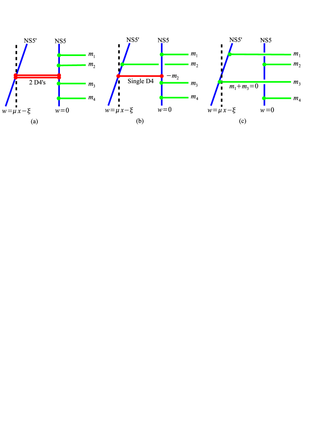
Figure 1: The classical brane configuration for $(N,N_{f})=(2,4)$. In general, the configuration has two finite D4-branes between the rotated NS5’-brane and NS5-brane, and four semi-infinite D4-branes from the right NS5-brane. The bullets on the line denote the end point of D4-branes on the NS5-brane. (a) Confining vacua. The number of vacua is 2. (b) Higgs vacua. There are 4 different choices in total. (c) “Baryonic” vacua for non-generic masses. The finite D4-branes disappear and brane configuration splits.

3 Integrable Systems and Vacuum Structure

3.1 The general story

In this section we set out a general picture of the relation between ${\cal N}=2$ theory broken to ${\cal N}=1$ and integrable systems. In this story it is very useful to have in mind the brane configurations of Type IIA string theory and brane rotation/deformation.

It is well-established that ${\cal N}=2$ theories are related to integrable systems [18]. The method that we describe in this section exploits this fact. The Seiberg-Witten curve of the theory is identified with the spectral curve of the integrable system. The moduli space, or Coulomb branch, of the theory, is therefore identified with the space of conserved quantities in the integrable system. The Coulomb branch has a natural set of coordinates which are defined by integrating the Seiberg-Witten holomorphic 1-form $\lambda$ around a set of canonical $A$-cycles on the curve $\Sigma$:

$$a_{i}=\oint_{A_{i}}\lambda\ .$$ (3.1)

Here, $i=1,\ldots,g$, the genus of $\Sigma$. The cycles are chosen so that the $a_{i}$ determine the masses of electrically changed BPS states int he theory. Magnetically charge BPS states involve the dual quantities

$$a_{i}^{D}=\oint_{B_{i}}\lambda\ ,$$ (3.2)

where the cycles $B_{i}$ are chosen to have intersections $A_{i}\cap B_{j}=\delta_{ij}$. Remarkably, the $a_{i}$ are precisely the action variables of the integrable system. The conjugate angle variables do not appear directly in the theory, however, they are identified with the coordinates $\psi_{i}$ of a point in the Jacobian of $\Sigma$. The Jacobian torus is defined as follows (for a reference on Riemann surfaces see [23]). Let $\omega_{j}$ be the associated set of $g$ holomorphic 1-forms (abelian differentials of the 1st kind) normalized so that $\oint_{A_{j}}\omega_{k}=\delta_{jk}$. The period matrix of $\Sigma_{\rm int}$ is the $g\times g$ matrix with elements

$$\tau_{jk}=\oint_{B_{j}}\omega_{k}\ .$$ (3.3)

The Jacobian torus consists of points $\psi_{j}\in{\bf C}^{g}$ with the identifications

$$\psi_{j}\thicksim\psi_{j}+n_{j}+\tau_{jk}m_{k}\ ,\qquad n_{j},m_{k}\in{\bf Z}\ .$$ (3.4)

As defined the $a_{i}$ and $\psi_{i}$ are canonically conjugate:

$$\{a_{i},\psi_{j}\}=\delta_{ij}\ .$$ (3.5)

In terms of the action angle variables, the dynamics with respect to any choice of Hamiltonian function $H(a_{i})$ is particularly simple:

$$\dot{a}_{i}=0\ ,\qquad\dot{\psi}_{i}=\frac{\partial H}{\partial a_{i}}\ .$$ (3.6)

We can be more explicit by using the fact that the spectral curve of the integrable system is described by a relation of the form $F(t,x)=0$ which is nothing but the usual description of the Seiberg-Witten curve of the field theory coming from the Type IIA brane configurations described in Section 2.2. In particular, the Seiberg-Witten 1-form is

$$\lambda=x\frac{dt}{t}\ .$$ (3.7)

An important rôle is played by the points $P_{i}$, $i=1,\ldots,k+1$, where $x=\infty$ at which $\Sigma$ is non-compact. In the brane configuration these are the points where one of the $k+1$ NS5-branes goes to infinity. In order to see their significance in the integrable system, let us consider the flows generated by some Hamiltonian at the level of the angles variables (3.6). It turns out that each flow can be written in terms of a meromorphic 1-form $\Omega$ on $\Sigma$ (actually an abelian differential of the 3rd kind) which is normalized by the condition

$$\oint_{A_{j}}\Omega=0\ .$$ (3.8)

The angular velocities are then given by integrals around the dual cycles:

$$\dot{\psi}_{i}=\oint_{B_{i}}\Omega\equiv\frac{\partial H}{\partial a_{i}}\$$ (3.9)

The 1-form $\Omega$ has poles at the points $P_{i}$ and the asymptotic expansions at these points are determined by the choice of Hamiltonian $H$:

$$\lim_{p\to P_{i}}\Omega(p)=d\big{(}U_{i}(x(p))+{\cal O}(1/x(p))\big{)}\ ,$$ (3.10)

where the $U_{i}(x)$ are polynomials which we will relate to the tree-level superpotentials which break ${\cal N}=2\to{\cal N}=1$. In fact in the brane picture $w=U_{i}(x)$ describes the bending of the $i^{\text{th}}$ NS5-brane in the 89 direction asymptotically at infinity. The ${\cal N}=1$ deformation of the $i^{\text{th}}$ gauge group factor is associated to a potential

$$W^{\prime}_{i}(x)=U_{i+1}(x)-U_{i}(x)\ .$$ (3.11)

Note that a shift in the $U_{i}(x)\to U_{i}(x)+f(x)$ is physically irrelevant. In the integrable system, the polynomials $U_{i}(x)$ determine specify $\Omega$ uniquely, up to exact terms which correspond to the freedom to shift each $U_{i}(x)$ by the same function. In this sense, only the differences of the $U_{i}(x)$ matter—as (3.11) makes clear.

We now relate $\Omega$, modulo exact terms, to $H$. The first move is to employ the Riemann’s bilinear relation to the abelian differentials

$$\pi_{i}\equiv\frac{\partial\lambda}{\partial a_{i}}$$ (3.12)

and $\Omega$:

$$\frac{1}{2\pi i}\sum_{i=1}^{g}\left(\oint_{A_{i}}\Omega\,\oint_{B_{i}}\pi_{j}-\oint_{B_{i}}\Omega\,\oint_{A_{i}}\pi_{j}\right)=\sum_{i=1}^{k}{\rm Res}_{P_{i}}(U_{i}(x)\pi_{j})\ ,$$ (3.13)

Now we use the normalization condition (3.8) and the fact that (3.1) and (3.12) imply that

$$\oint_{A_{i}}\pi_{j}=\delta_{ij}\ ,$$ (3.14)

to deduce

$$-\oint_{B_{i}}\Omega=\sum_{i=1}^{k+1}{\rm Res}_{P_{i}}(U_{i}(x)\pi_{i})=\frac{\partial}{\partial a_{i}}\sum_{i=1}^{k+1}{\rm Res}_{P_{i}}(U_{i}(x)\log t\,dx)\ .$$ (3.15)

In the last line we used the fact that the $a_{i}$ derivative is at constant $x$ and so could be pulled outside the integral. Hence, by comparing this with (3.6) we deduce that

$$H=-\sum_{i=1}^{k}{\rm Res}_{P_{i}}(U_{i}(x)\log t\,dx)$$ (3.16)

At this point we can investigate the equilibrium configurations of the integrable system which ought, by our general reasoning, to be associated to vacua of the QFT. For an equilibrium,

$$\frac{\partial H}{\partial a_{i}}=0\ \implies\ \oint_{B_{i}}\Omega=0\ .$$ (3.17)

Given the normalization condition this implies that for an equilibrium $\Omega=dw$, for some meromorphic function $w$ with singularities at $P_{i}$ with asymptotic behaviour from (3.10), $w\to U_{i}(x)+\cdots$. Hence the existence of a vacuum of the gauge theory can be phrased as the existence of a certain meromorphic function on the curve of the theory. The relation to the brane configuration should now be obvious. The points $P_{i}$, as we have said, represent the asymptotic positions of the NS5-branes. The meromorphic function $w$ describes the deformation of the Seiberg-Witten curve into the 89-plane associated with the breaking of ${\cal N}=2$ to ${\cal N}=1$. The superpotential (3.16) at the critical point can be written as an integral over the Riemann surface

$$H^{\star}=-\frac{1}{2\pi i}\int_{\Sigma}\log t\,dw\wedge dx\ ,$$ (3.18)

from which one can relate to Witten’s MQCD superpotential [24] (see [4] for a discussion of the relation).

For our particular example, there are two NS5-branes and hence two points at infinity $P_{1}\equiv\infty^{+}$ and $P_{2}=\infty^{-}$. We can choose $U_{2}=0$ and $U_{1}(x)=W^{\prime}(x)$. By integrating-by-parts in (3.16), we have a Hamiltonian and hence an effective superpotential

$$W_{\text{int}}=\text{Res}_{\infty^{+}}\Big{(}W(x)\frac{dt}{t}\Big{)}\ ,$$ (3.19)

Notice that we have developed the theory of the integrable system entirely in the language of action/angle variables. However, for certain examples we can write down the Hamiltonians in terms of other kinds of variables; for instance, the positions and momenta of particles, or spin variables and mixtures thereof. We do this for the theory with $N_{f}=2N$ fundamental hypermultiplets in the next section.

3.2 Spin Chains

In this section, we describe how to extend the integrable system approach to describe the ${\cal N}=2$ theories with fundamental matter. The integrable system that is associated to the finite theory, with $N_{f}=2N$, has been identified in [15, 16, 17, 18] as a certain twisted $SU(2)$ spin chain. This system describes the interactions of a set $N$ spins $\vec{S}^{(i)}$, $i=1,\ldots,N$, which are 3-vectors

$$\vec{S}^{(i)}=\big{(}S^{(i)}_{1},S^{(i)}_{2},S^{(i)}_{3}\big{)}\ .$$ (3.20)

The overall length of each vector is non-dynamical:

$$\vec{S}^{(i)}\cdot\vec{S}^{(i)}=k_{i}^{2}\ .$$ (3.21)

The parameters $k_{i}$ will be associated to masses in due course.

The integrable system has a $2\times 2$ “Lax matrix” defined at each “site”:

$$L_{i}(x)=\begin{pmatrix}x+\lambda_{i}+S^{(i)}_{3}&S^{(i)}_{1}-iS^{(i)}_{2}\\ S^{(i)}_{1}+iS^{(i)}_{2}&x+\lambda_{i}-S^{(i)}_{3}\end{pmatrix}$$ (3.22)

The “transfer matrix” is then defined to be

$$T(x)=L_{1}(x)\cdots L_{N}(x)V$$ (3.23)

and we have allowed for a “twisting” described by the constant matrix $V$. Unlike [15, 16, 17, 18], we will make the choice

$$V=\begin{pmatrix}-h&0\\ 0&h+2\end{pmatrix}\ ,$$ (3.24)

where $h$ is a parameter that we will relate to the UV coupling of the theory. The integrable system has a spectral curve $\Sigma$ defined by the algebraic relation between $x$ and another variable $t$:

$$F(x,t)=\det\big{(}T(x)-t{\bf 1}\big{)}=0\ .$$ (3.25)

This curve is easily seen to have genus $N-1$. The relation between the spectral curve and the integrable system is well known. The moduli space of the curve parameterizes the space of conserved quantities of the system. There are $3N$ variables subject to $N$ constraints (3.21); hence, the dimension of the phase space is $2N$. In particular, the action variables are given by integrating the 1-form $xd\log t$ around a set of basis 1-cycles on the curve. The conjugate angle variables are associated to a point in the Jacobian of $\Sigma$.

The curve $\Sigma$ has the form

$$t^{2}-2tP(x)-h(h+2)Q(x)=0\ ,$$ (3.26)

where

$$Q(x)=\prod_{I=1}^{2N}(x-m_{I})$$ (3.27)

with

$$m_{2i-1}=-\lambda_{i}-k_{i}\ ,\qquad m_{2i}=-\lambda_{i}+k_{i}\ ,$$ (3.28)

$i=1,\ldots,N$, and where

$$P(x)=x^{N}+H_{1}x^{N-1}+H_{2}x^{N-2}+\cdots+H_{N}\ .$$ (3.29)

Notice that the form of the curve is identical to the Seiberg-Witten curve of the ${\cal N}=2$ theory with $SU(N)$ gauge group and $N_{f}=2N$ fundamental hypermultiplets, and where $h$ is expressed in terms of the coupling by [25, 26]

$$h(\tau)=\frac{2\lambda(\tau)}{1-2\lambda(\tau)}\ ,$$ (3.30)

where $\lambda(\tau)$ involves the automorphic function

$$\lambda(\tau)=16q\prod_{n=1}^{\infty}\left(\frac{1+q^{2n}}{1+q^{2n-1}}\right)^{8}\ ,$$ (3.31)

and $q=e^{\pi i\tau}$. In particular, at weak coupling $h=32q+\cdots$. The parameters $m_{I}$ in (3.27) are not directly the bare masses, in fact

$$m_{I}=m_{I}^{b}+h\sum_{I=1}^{2N}m_{I}^{b}/(2N)\ .$$ (3.32)

In addition, the coupling $\tau$ in the curve is not equal to the bare coupling of the theory [19]. In general they are related by an instanton expansion of the form (1.2).

In (3.29) the $H_{i}(\vec{S}^{(j)})$ are a basis for the Hamiltonians of the integrable system. Explicitly, the first two Hamiltonians are

$$H_{1}=\sum_{i}\big{(}\lambda_{i}-(1+h)S^{(i)}_{3}\big{)}$$ (3.33)

and

$$H_{2}=\sum_{i<j}\Big{(}\lambda_{i}\lambda_{j}+i(1+h)\big{(}S^{(i)}_{2}S^{(j)}_{1}-S^{(i)}_{1}S^{(j)}_{2}\big{)}+\vec{S}^{(i)}\cdot\vec{S}^{(j)}-(1+h)\big{(}\lambda_{i}S^{(j)}_{3}+\lambda_{j}S^{(i)}\big{)}\Big{)}\ .$$ (3.34)

3.3 Breaking to ${\cal N}=1$

Now that we have established the precise relation between the twisted spin chain and the ${\cal N}=2$ field theory, we now consider the problem of breaking to ${\cal N}=1$ using the integrable system. The procedure is well established [10, 11]. First of all, consider compactifying the theory to three dimensions on a circle of finite radius $R$. In the 3-dimensional effective theory, the gauge field in the $U(1)^{N-1}$ unbroken gauge group can be “dualized” to scalar fields. These fields, along with the Wilson lines of the $U(1)^{N-1}$ around the circle amass into complex scalar field. The $N-1$ complex scalar fields are then naturally valued on a complex torus; in fact, precisely the Jacobian torus of $\Sigma$. In summary the Coulomb branch of the theory in three dimensions is identified with the complexified phase space of the integrable system and the split between the action-angle variables describes the moduli of the Coulomb branch of the four-dimensional theory plus the dual photons and Wilson lines.

Breaking to ${\cal N}=1$, as in (1.1), is described by an effective superpotential on the Coulomb branch of the 3-dimensional theory. The resulting superpotential is simply, as described in the last section in detail, one of the Hamiltonians of the integrable system. From (3.19), we have the following expression for the effective superpotential

$$W_{\text{int}}=\text{Res}_{\infty^{+}}W(x)\frac{dt}{t}=\text{Res}_{\infty^{+}}W(x)\left(\frac{P^{\prime}}{y}+\frac{h(h+2)Q^{\prime}}{2y(y+P)}\right)\ .$$ (3.35)

In particular, since $W(x)$ contains the term $-\xi x$ we have the constraint

$$\text{Res}_{\infty^{+}}x\left(\frac{P^{\prime}}{y}+\frac{h(h+2)Q^{\prime}}{2y(y+P)}\right)=0\ .$$ (3.36)

This can be written

$$H_{1}(\vec{S}^{(j)})=\frac{h}{2}\sum_{I=1}^{2N}m_{I}=-(\lambda_{1}+\lambda)h\ .$$ (3.37)

At the level of the integrable system experience with the finite $U(N)^{k}$ quiver theories [11], where the relative $U(1)$ factor are also IR free, suggests that the correct way to freeze out the $U(1)$ factor is via a Hamiltonian reduction. So as well as imposing (3.37) on the phase space, one also takes a quotient by the conjugate variable to $H_{1}$. Notice that $H_{1}$ generates a simultaneous rotation of the spins $\vec{S}^{(i)}$ around the $S^{(i)}_{3}$ axes and so the conjugate variable is this angle. In practice it is easier not to perform the quotient explicitly and as a consequence we shall find a degeneracy in our critical points corresponding to this unwanted degree-of-freedom.

3.4 Example: $SU(2)$

In this section, we consider the vacuum structure for the case of gauge group $SU(2)$ and the quadratic mass deformation $W(x)=\mu x^{2}/2-\xi x$. After imposing the constraint, and using (3.35), we find an effective superpotential

$$W_{\text{int}}=-\frac{\mu(H_{2}+h\sum_{I<J}m_{I}m_{J}/2)}{2(h+1)}\ .$$ (3.38)

So vacua are given by critical point of $H_{2}$. First of all, we solve the constraint (3.37) explicitly by choosing

$$S^{(1)}_{3}=y\ ,\qquad S^{(2)}_{3}=\lambda_{1}+\lambda_{2}-y\ .$$ (3.39)

and then impose the constraints (3.21) with Lagrange multipliers $\xi_{i}$, $i=1,2$. In order the that the four equations that result from the derivatives of $H_{2}$ with respect to $S^{(1)}_{1,2}$ and $S^{(2)}_{1,2}$, do not imply that the four aforementioned variables vanish (which would not be compatible with the constraints (3.21)), we need

$$\xi_{1}\xi_{2}+\frac{h(h+2)}{4}=0\ .$$ (3.40)

From this we find

$$S^{(1)}_{1}=\frac{-S^{(2)}_{1}+i(1+h)S^{(2)}_{2}}{2\xi_{1}}\ ,\qquad S^{(1)}_{2}=\frac{-i(1+h)S^{(2)}_{1}-S^{(2)}_{2}}{2\xi_{1}}\ .$$ (3.41)

The equation $\partial H_{2}/\partial y=0$ can then be solved for $y$. This leaves the two constraints (3.21) which imply that the Lagrange multiplier $\xi_{1}$ satisfies a sixth-order polynomial equation

$$\begin{split}&-64k_{1}^{2}\xi_{1}^{6}+128k_{1}^{2}\xi_{1}^{5}+16(2(h^{2}+2h-2)k_{1}^{2}+4\lambda_{1}^{2}+h(-2k_{2}^{2}+6\lambda_{1}^{2}+2\lambda_{2}^{2})+\\ &h^{2}(-k_{2}^{2}+2\lambda_{1}+2\lambda_{2}^{2}))\xi_{1}^{4}+32h(h+2)(-k_{1}^{2}+k_{2}^{2}(1+h)(\lambda_{1}^{2}-\lambda_{2}^{2}))\xi_{1}^{3}\\ &+4h(h+2)(-h(h+2)k_{1}^{2}+2((h^{2}+2h-2)k_{2}^{2}+(h+1)(2\lambda_{2}^{2}+h(\lambda_{1}^{2}+\lambda_{2}^{2}))))\xi_{1}^{2}\\ &-8h^{2}(h+2)^{2}k_{2}^{2}\xi_{1}-h^{3}(h+2)^{3}k_{2}^{2}=0\ .\end{split}$$ (3.42)

Note that each of the 6 solutions is degenerate due to simultaneous rotations in the $(S^{(1)}_{1},S^{(1)}_{2}$ and $(S^{(2)}_{1},S^{(2)}_{2})$ planes. However, this is the expected and unphysical degeneracy in the conjugate variable to $H_{1}$.

So the final result is that there are six vacua, which is the number expected (2.14). For generic values of the parameters it is not possible to write down explicitly the critical value of the superpotential. However, let us consider their weak coupling, $h\to 0$ limit. There are three pairs of solutions:

(i) $\xi_{1}=1\pm\lambda_{1}/k_{1}+{\cal O}(h)$ and $\xi_{2}={\cal O}(h)$, which gives

$$\begin{split}\vec{S}^{(1)}&=\Big{(}-\frac{\sigma-i\eta}{2(1\pm\lambda_{1}/k_{1})},\frac{-i\sigma-\eta}{2(1\pm\lambda_{1}/k_{1})},\mp k_{1}\Big{)}+{\cal O}(h)\ ,\\ \vec{S}^{(2)}&=\Big{(}\sigma,\eta,\lambda_{1}+\lambda_{2}\pm k_{1}\Big{)}+{\cal O}(h)\ ,\end{split}$$ (3.43)

where $\sigma^{2}+\eta^{2}=k_{2}^{2}-(\lambda_{1}+\lambda_{2}\pm k_{1})^{2}$.

(ii) $\xi_{1}={\cal O}(h)$ and $\xi_{2}=1\pm\lambda_{2}/k_{2}+{\cal O}(h)$, which gives

$$\begin{split}\vec{S}^{(1)}&=\Big{(}\xi,\eta,\lambda_{1}+\lambda_{2}\pm k_{2}\Big{)}+{\cal O}(h)\ ,\\ \vec{S}^{(2)}&=\Big{(}-\frac{\sigma-i\eta}{2(1\pm\lambda_{2}/k_{2})},\frac{-i\sigma-\eta}{2(1\pm\lambda_{2}/k_{2})},\mp k_{2}\Big{)}+{\cal O}(h)\ ,\end{split}$$ (3.44)

where $\xi^{2}+\eta^{2}=k_{1}^{2}-(\lambda_{1}+\lambda_{2}\pm k_{2})^{2}$.

(iii) $\xi_{1}=\pm((k_{2}^{2}-\lambda_{2}^{2})h/2(\lambda_{1}^{2}-k_{1}^{2}))^{1/2}+{\cal O}(h)$, which gives

$$\begin{split}\vec{S}^{(1)}&=\Big{(}-\frac{\sigma-i\eta}{2\xi_{1}},\frac{-i\sigma-\eta}{2\xi_{1}},\lambda_{1}\Big{)}+{\cal O}(h)\ ,\\ \vec{S}^{(2)}&=\Big{(}\sigma,\eta,\lambda_{2}\Big{)}+{\cal O}(h)\ ,\end{split}$$ (3.45)

where $\sigma^{2}+\eta^{2}=\lambda_{2}^{2}$.

In all these solutions the degeneracy due to rotations in $(\xi,\eta)$ corresponds to the angle variable conjugate to $H_{1}$ and is not physically relevant. Clearly the four vacua (i) and (ii) are the Higgs vacua with an expansion in instantons $h\sim e^{\pi i\tau}$ at weak coupling. For these vacua we can write the first two terms in the weak coupling expansion as

$$W^{*}_{\text{int}}=\mu m_{I}^{2}-\frac{\mu\prod_{J=1}^{4}(m_{I}+m_{J})}{8m_{I}^{2}}h+{\cal O}(h^{2})$$ (3.46)

The two vacua (iii) are identified with the confining vacua since they have an expansion in terms of $h^{1/2}$, in other words, finite instantons, at weak coupling. In these vacua

$$W^{*}_{\text{int}}=\pm 2\mu\big{(}m_{1}m_{2}m_{3}m_{4}h/2\big{)}^{1/2}+{\cal O}(h)\ .$$ (3.47)

These results may be checked very directly by factorizing the Seiberg-Witten curve. Defining the curve as

$$G(x,t)=t-2P(x)-h(h+2)Q(x)/t\ .$$ (3.48)

For the $SU(2)$ case this genus one curve degenerates to genus zero when

$$\frac{\partial G}{\partial t}=\frac{\partial G}{\partial x}=0\ .$$ (3.49)

These equations can be reduced to a single sixth-order polynomial equation for $x$:

$$h(h+2)Q^{\prime}(x)^{2}+4Q(x)P^{\prime}(x)^{2}=0\ ,\qquad t=-h(h+2)\frac{Q^{\prime}(x)}{2P^{\prime}(x)}\ .$$ (3.50)

The six solutions correspond to the four Higgs and two confining vacua and one can verify the result above.

4 The Holomorphic Matrix Model

The effective superpotential of our supersymmetric field theory can also be calculated from a holomorphic matrix model in the way describing originally by Dijkgraaf and Vafa [27] and then extended to include fundamental matter in [28] (see also the review [5] and references therein).

The matrix model is defined by the partition function

$$Z=\int[d\hat{\Phi}][d\hat{Q}][d\hat{\tilde{Q}}]e^{-\frac{1}{g_{s}}W_{\rm tree}(\hat{\Phi},\hat{Q},\hat{\tilde{Q}})}\ ,$$ (4.1)

where $W_{\rm tree}(\hat{\Phi},\hat{Q},\hat{\tilde{Q}})$ has the same form as the field theoretical tree level superpotential, but each $\hat{\Phi}$, $\hat{Q}$ and $\hat{\tilde{Q}}$ are now $\hat{N}\times\hat{N}$, $\hat{N}\times N_{f}$ and $N_{f}\times\hat{N}$ matrices, respectively, not fields. Here $\hat{N}$ is a number of “colors” to be taken the large $\hat{N}$ with fixed physical quantities of $N$, $N_{f}$ and $S=g_{s}\hat{N}$. The integral is to be understood in a holomorphic sense.

The matrices $\hat{Q}$ and $\hat{\tilde{Q}}$ appear quadratically and can be integrated out. Gauge transformation can then be used to diagonalize $\Phi$ at the expense of introducing a gauge-fixing determinant—the Vandermonde determinant. Denoting the eigenvalues of $\Phi$ as $\lambda_{i}$, $i=1,2,\ldots,\hat{N}$, the partition function becomes

$$Z=\int\prod_{i=1}^{N}d\lambda_{i}\,\frac{\prod_{i\neq j}(\lambda_{i}-\lambda_{j})}{\prod_{I=1}^{N_{f}}\prod_{i=1}^{N}(\lambda_{i}-m_{I})}e^{-\frac{1}{g_{s}}\sum_{i=1}^{N}W(\lambda_{i})}.$$ (4.2)

We now take the limit $\hat{N}\to\infty$ and $g_{s}\to 0$ with $S=g_{s}\hat{N}$ fixed. In this limit, it is appropriate to introduce a density of eigenvalues

$$\rho(\lambda)=\frac{1}{\hat{N}}\sum_{i=1}^{\hat{N}}\delta(\lambda-\lambda_{i}),$$ (4.3)

which is normalized as

$$\int d\lambda\,\rho(\lambda)=1\ .$$ (4.4)

The free-energy of the model has the expansion

$$-\ln Z=\frac{1}{g_{s}^{2}}{\cal F}_{\chi=2}+\frac{1}{g_{s}}{\cal F}_{\chi=1}\ ,$$ (4.5)

where

$${\cal F}_{\chi=2} =S\int d\lambda\,\rho(\lambda)W(\lambda)-S^{2}\int d\lambda d\lambda^{\prime}\,\rho(\lambda)\rho(\lambda^{\prime})\log(\lambda-\lambda^{\prime})\ ,$$ (4.6a)

$${\cal F}_{\chi=1} =S\sum_{I=1}^{N_{f}}\int d\lambda\,\rho(\lambda)\log(\lambda-m_{I}),$$ (4.6b)

are a contribution from the planer diagrams (sphere) and diagram with one boundary, respectively.

To leading order, the density of eigenvalues is determined from the saddle-point equation

$$2\int d\lambda^{\prime}\frac{\rho(\lambda^{\prime})}{\lambda-\lambda^{\prime}}=\frac{1}{S}W^{\prime}(\lambda)\ .$$ (4.7)

In the classical limit ($S\to 0$), the eigenvalues sit at one of the critical points of $W(x)$. In other words, a classical configuration of eigenvalues can be described by the filling fraction $\hat{N}_{i}/\hat{N}$ of the $i^{\text{th}}$ critical point. We are assuming that $W(x)$ is a polynomial of degree $n+1$. However, the saddle-point equation includes interaction terms coming from the Vandermonde determinant as well as from integrating out the matter matrices. At this point, we apply the usual hypothesis which states that the effect of these terms is to pull the eigenvalues away from the critical points along a set of open contours ${\cal C}_{i}$, $i=1\,\ldots,n$, in the neighbourhood of each critical point. The saddle-point equations (4.7) can be solved by introducing a resolvent

$$\omega(x)=\int_{{\cal C}}d\lambda\,\frac{\rho(\lambda)}{x-\lambda}\ ,$$ (4.8)

where ${\cal C}=\cup_{i=1}^{n}{\cal C}_{i}$. Note that $\omega(x)$ is an analytic function over the complex plane with cuts along ${\cal C}_{i}$. The density can be recovered from $\omega(x)$ as the discontinuity across the cuts ${\cal C}$:

$$\omega(x+\epsilon)-\omega(x-\epsilon)=-2\pi i\rho(x)\ ,\quad x\in{\cal C}\ ,$$ (4.9)

where $\epsilon$ is a suitable infinitesimal, so that $x\pm\epsilon$ lie just above and below the cut, respectively. In terms of $\omega(x)$, the saddle-point equation becomes

$$\omega(x+\epsilon)+\omega(x-\epsilon)=\frac{1}{S}W^{\prime}(x)\ ,\qquad x\in{\cal C}\ .$$ (4.10)

Since $\omega(x)$ goes to 0 at infinity, the solution to the saddle-point equation (4.10) is immediate:

$$2S\omega(x)=W^{\prime}(x)-\sqrt{W^{\prime}(x)^{2}+f(x)}\ ,$$ (4.11)

where $f(x)$ is an arbitrary polynomial of degree $n-1$. This latter requirement ensures

$$\lim_{x\to\infty}2S\omega(x)={\cal O}(1/x)\ .$$ (4.12)

It is useful to define

$$y^{2}=\big{(}W^{\prime}(x)-2S\omega(x)\big{)}^{2}=W^{\prime}(x)^{2}+f(x)\ .$$ (4.13)

The two sheets of $y$ describe a hyper-elliptic Riemann surface $\Sigma_{\text{mm}}$ with genus—at least generically—of $n-1$.

The $k$ constants in $f(x)=\sum_{j=1}^{n}b_{j}x^{j-1}$ are the moduli of the saddle-point solution, i.e. of the auxiliary surface $\Sigma_{\text{mm}}$. These $k$ moduli represent the freedom to choose the $k$ filling fractions at each cut and we may change variables $\{b_{i}\}\to\{S_{i}\}$, where

$$S_{i}=g_{s}\hat{N}_{i}=\int_{{\cal C}_{i}}\rho(x)dx=-\frac{1}{4\pi i}\oint_{A_{i}}y(x)dx\ ,$$ (4.14)

where $A_{i}$ is a contour which encloses the cut ${\cal C}_{i}$. In particular,

$$S=\sum_{i=1}^{n}S_{i}=-\sum_{i=1}^{n}\frac{1}{4\pi i}\oint_{A_{i}}\,y(x)dx=\frac{1}{4\pi i}\oint_{\infty^{+}}y(x)\,dx=-\frac{b_{N}}{4\mu_{N+1}}\ ,$$ (4.15)

where we pulled the contour off the cuts to the point at infinity $\infty^{+}$ on the top sheet ($y=\sqrt{W^{\prime}(x)^{2}+f(x)}$).

We now have all the ingredients to define the glueball superpotential which is the effective superpotential of the physical field theory, in a particular classical vacuum, where the $S_{i}$ are interpreted as fields:

$$W_{\rm gb}=\sum_{i=1}^{n}\left(N_{i}\frac{\partial{\cal F}_{\chi=2}}{\partial S_{i}}+\pi i\tau S_{i}\right)+{\cal F}_{\chi=1}\ .$$ (4.16)

Here, $\tau$ is the bare coupling of the field theory and the classical vacuum is specified by the $N_{i}$, $\sum_{i=1}^{n}N_{i}=N$, the number of eigenvalues of the adjoint field $\Phi$ lying at the $i^{\text{th}}$ critical point of $W(x)$.

To evaluate the derivative of ${\cal F}_{\chi=2}$ in (4.16), one can relate it to the variation of the free energy in bringing an eigenvalue in from infinity to the point $e_{i}$ at the end of the $i^{\text{th}}$ cut. Since the force on eigenvalue is $y$ we have

$$\frac{\partial{\cal F}_{\chi=2}}{\partial S_{i}}=\int_{\infty^{+}}^{e_{i}}y\,dx\ .$$ (4.17)

The contribution from the matter fields, the third term in (4.16), is easily evaluated, again one can show [29]

$${\cal F}_{\chi=1}=\tfrac{1}{2}\sum_{I=1}^{N_{f}}\Big{(}-\int^{\infty^{-}}_{m_{I}}y\,dx+W(m_{I})\Big{)}\ .$$ (4.18)

In (4.17) and (4.18), the integrals are actually divergent at infinity and need to be regularized. However, since we will work ultimately in the finite theory where the divergences cancel we shall not explicitly describe the details of the regularization process. In (4.18), the point with $x=m_{I}$ can be either on the top or bottom sheet of $\Sigma$ and this freedom to choose is necessary in order to describe all the vacua of the physical theory [29]. Since we will later choose all the $m_{I}$ on the bottom sheet when we engineer the Seiberg-Witten curve, we take the integral out to the point at infinity on the bottom sheet. If we need to specify whether $x=m_{I}$ is on the top or bottom sheet we write $m^{\pm}_{I}$, respectively.

Using (4.17) and (4.18), the glueball superpotential (4.16) takes the form

$$W_{\rm gb}=-\sum_{i=1}^{n}N_{i}\int_{e_{i}}^{\infty^{+}}y\,dx-\frac{\tau}{4}\sum_{i=1}^{n}\oint_{A_{i}}y\,dx-\tfrac{1}{2}\sum_{I=1}^{N_{f}}\left(\int_{m_{I}}^{\infty^{-}}y\,dx-W(m_{I})\right)\ .$$ (4.19)

We now specialize to the case $N_{f}=2N$ and in this case the potential divergences at the infinite points cancel and the regular can be removed.

4.1 Engineering the Seiberg-Witten curve

The Seiberg-Witten curve itself can be extracted from the matrix model by choosing a suitably generic potential $W(x)$ with order $N+1$:

$$W^{\prime}(x)=\mu_{N+1}\prod_{i=1}^{N}(x-\zeta_{i})\ .$$ (4.20)

This potential acts as a probe for the ${\cal N}=1$ vacuum which can zero-in on any point on the Coulomb branch of the ${\cal N}=2$ theory.

The matrix model curve $\Sigma_{\text{mm}}$ for an $N$-cut solution at the critical point of the glueball superpotential, with one physical eigenvalue at each critical point $N_{i}=1$, is then identified with the Seiberg-Witten curve where the $\{\zeta_{i}\}$ are related to the moduli $\{a_{i}\}$ of the ${\cal N}=2$ Coulomb branch as in (3.26). In addition the points $x=m_{I}$ are taken on the bottom sheet, which we indicate as $m^{-}_{I}$. We now proceed to find the critical point of the glueball superpotential in this case.

It is important for what follows that the $N-1$ quantities

$$\frac{\partial}{\partial b_{i}}y\,dx=\frac{x^{i-1}}{2y}\,dx\ ,$$ (4.21)

for $i=1,\ldots,N-1$, form a basis for the abelian differentials of the first kind on $\Sigma$. We will choose another basis for the abelian differentials $\{\omega_{i}\}$, $i=1\ldots,N-1$, normalized by

$$\oint_{A_{i}}\omega_{j}=\delta_{ij}\ ,\quad i,j=1,\ldots,N-1\ .$$ (4.22)

In addition,

$$\frac{\partial}{\partial b_{i}}y\,dx=\frac{1}{2\mu_{N+1}}\tau_{\infty^{+}\infty^{-}}\ ,$$ (4.23)

where on the right-and side we have $\tau_{p_{1}p_{2}}$, the meromorphic 1-form with simple poles at $p_{1}$ and $p_{2}$ with residues $\mp 1$, respectively.

The glueball superpotential (4.19) (with $N_{i}=1$ and $N_{f}=2N$) can be written

$$W_{\text{gb}}=-\frac{1}{2}\sum_{i=1}^{N}\int_{\hat{B}_{i}}y\,dx-\frac{\pi i\tau}{4\mu_{N+1}}b_{N}-\frac{1}{2}\sum_{I=1}^{2N}\left(\int_{m_{I}^{-}}^{\infty^{-}}y\,dx-W(m_{I})\right)\ ,$$ (4.24)

where $\hat{B}_{i}$ is the contour that goes from $\infty^{-}$ through the $i^{\text{th}}$ cut to $\infty^{+}$. To reach this expression we used the fact that $\int_{e_{i}}^{\infty^{+}}y\,dx=\tfrac{1}{2}\int_{\hat{B}_{i}}y\,dx$. As we have already explained this expression must be regularized, although at the end in the $N_{f}=2N$ case the regulator can be removed. The careful treatment of the regularization process is given in [29].

Figure 2: The integral paths for the effective superpotential calculation. The curve has two sheets connecting $N$ cuts and there are two distinguish infinite points, which we denote $\infty^{+}$ and $\infty^{-}$. The integral cycles are defined in the figure.

Taking the derivative of (4.24) with respect to $b_{i}$, $i=1,\ldots,N-2$, (we will consider the $b_{N-1}$ equation below) and taking suitable linear combinations to change basis between $\{x^{i}dx/y\}$ and $\{\omega_{i}\}$, we have

$$0=-\sum_{j=1}^{N}\int_{\hat{B}_{j}}\omega_{i}-\sum_{I=1}^{2N}\int_{m_{I}^{-}}^{\infty^{-}}\omega_{i}=-N\int_{\infty^{-}}^{\infty^{+}}\omega_{i}-\sum_{I=1}^{2N}\int_{m_{I}^{-}}^{\infty^{-}}\omega_{i}\ ,$$ (4.25)

where in the last line we have equality up to an element of the Jacobian lattice, $p_{i}+\tau_{ij}q_{j}$, $p_{i},q_{i}\in\mathbb{Z}$.

According to Abel’s theorem, (4.25) implies that there exists a meromorphic function on $\Sigma$ with a divisor $(\infty^{+})^{-N}(\infty^{-})^{-N}m_{1}^{-}\cdots m_{2N}^{-}$. This function is explicitly

$$t=P(x)+y\ ,$$ (4.26)

where $P(x)=\prod_{i=1}^{N}(x-a_{i})$ is a polynomial of degree $N$. In order that $t$ has zeros at $x=m_{I}$ on the bottom sheet implies that

$$P(x)+\gamma Q(x)=W^{\prime}(x)^{2}+f(x)\ .$$ (4.27)

where $Q(x)=\prod_{I=1}^{2N}(x-m_{I})$. These are $2N$ equations that determine $\{a_{i},b_{i}\}$. There is one remaining unknown $\gamma$ which will be fixed below. Hence, at the critical point the curve can be written

$$y^{2}=P(x)^{2}+\gamma Q(x)\ ,$$ (4.28)

We recognize this as precisely the Seiberg-Witten curve (3.26) and in particular the $\{a_{i}\}$ are the moduli on the Coulomb branch.

The remaining equation is obtained by taking the derivative with respect to $b_{N}$. After using a Riemann bilinear relation with $d\log t$ and $\partial(y\,dx)/\partial b_{N-1}$ one obtains

$$\tau=\frac{t(\infty^{-})}{t(\infty^{+})}=\frac{1}{\pi i}\log\frac{1-\sqrt{1+\gamma}}{1+\sqrt{1+\gamma}}\ .$$ (4.29)

Note that this expression, for the case $N_{f}<2N$, requires regularization, however, in the finite theory this is not necessary and a finite answer is obtained. Expressing $\gamma=h(h+2)$, as in (3.26), we find

$$h=-\frac{2e^{\pi i\tau}}{1+e^{\pi i\tau}}\ .$$ (4.30)

Comparing with (3.30), we see that the matrix model coupling, which we now denote as $\tau_{\text{mm}}$, cannot be equal to the Seiberg-Witten coupling $\tau_{\text{SW}}$ directly, rather they are related by an expression of the form (1.2).

We can now see that the matrix model approach to the vacuum problem agrees precisely with the integrable system treatment. Firstly the matrix model curve and Seiberg-Witten curve are identical, (3.26) and (4.28). Secondly one can compare the critical value of the superpotential. Using once again a Riemann bilinear identity for $d\log t$ and $y\,dx$ one finds that the critical value of the glueball superpotential is

$$W^{*}_{\text{gb}}={\rm Res}_{\infty^{+}}\Big{(}W(x)\frac{dt}{t}\Big{)}$$ (4.31)

a result that agrees precisely with $W^{*}_{\text{int}}$ in (3.19).

4.2 Effective superpotential for the quadratic potential

In this section, we analyze the effective superpotential for the quadratic potential $W(x)=\mu x^{2}/2$. This corresponds to looking at the one cut solution of the matrix model. Actually, in order to compare with the results of Section 3.2 we have to take into account the behaviour of the overall $U(1)$ factor. The matrix model calculation on the face of it involves the gauge group $U(N)$ rather than $SU(N)$. However, the $U(1)$ factor is, as we have described earlier, actually frozen out and is non-dynamical. However, in the matrix model approach the trace of $\Phi$ is non-vanishing. One finds

$$\langle{\rm Tr}\,\Phi\rangle=\sum_{j=1}^{r}m_{I_{j}}\ .$$ (4.32)

In order to compare with our earlier results we can force the trace part of $\Phi$ to vanish by considering, as previously, a more general potential $W(x)=\mu x^{2}/2-\xi x$. The extra parameter $\xi$ acts as a Lagrange multiplier which will be fixed by varying the effective superpotential.

The second question that confronts us is how the one cut solution can describe the multiplicity of vacua that we described in Section 2. The origin for the multiplicity of vacua is solved by realizing that there is an ambiguity as to which sheet the points $m_{I}$ lie. It is useful at this point to compare to brane configurations in Section 2.2. If $m_{I}$ lies on the bottom sheet then we interpret this to mean in brane language that the corresponding semi-infinite D4-brane ends on the right-hand NS5-brane, while, conversely, $m_{I}$ lies on the top sheet then the semi-infinite D4-brane ends on the left-hand NS5-brane. This means that the confining vacua, for example, have all the $m_{I}$ on the bottom sheet.

For the one-cut solution, $y^{2}=(\mu x-\xi)^{2}+b_{1}$ and the glueball superpotential is

$$W_{\rm gb}=\frac{\pi i\tau}{4\mu}b_{1}-\frac{1}{2}\sum_{I=1}^{2N}\Big{(}\int_{m_{I}}^{e_{1}}y\,dx-W(m_{I})\Big{)}\ ,$$ (4.33)

where $e_{1}$ is a point at the end of the cut. We can evaluate the integrals in this expression explicitly to give

$$W_{\rm gb}=\frac{\pi i\tau}{4\mu}b_{1}+\frac{1}{4\mu}\sum_{I=1}^{2N}\Big{(}\mu^{2}m_{I}^{2}-2\xi m_{I}+\mu\tilde{m}_{I}f_{\pm}(\tilde{m}_{I})+b_{1}\log\big{(}\mu\tilde{m}_{I}+f_{\pm}(\tilde{m}_{I})\big{)}-\tfrac{1}{2}b_{1}\log(-b_{1})\Big{)}$$ (4.34)

where we have defined $\tilde{m}_{I}=m_{I}-\xi/\mu$. Note that $f_{\pm}(x)=\pm\sqrt{\mu^{2}x^{2}+b_{1}}$ depending upon whether $x$ is on the top or bottom sheet, respectively.

The critical point equation is

$$\prod_{I=1}^{2N}\big{(}\mu\tilde{m}_{I}+f_{\pm}(\tilde{m}_{I})\big{)}=(-b_{1})^{N}e^{\pi i\tau}\ .$$ (4.35)

the critical value of the glueball superpotential is then

$$W_{\text{gb}}^{*}=\frac{1}{4\mu}\sum_{I=1}^{2N}\big{(}\mu^{2}m_{I}^{2}-2\xi m_{I}+\mu\tilde{m}_{I}f_{\pm}(\tilde{m}_{I})\big{)}\ .$$ (4.36)

4.3 The vacuum structure

In Section 2, we labelled the vacua by a subset $\{m_{I_{1}},\ldots,m_{I_{r}}\}\subset\{m_{1},\ldots,m_{2N}\}$. We will identify this vacuum with the matrix model saddle-point solution where $\{m_{I_{1}},\ldots,m_{I_{r}}\}$ are on the top sheet and the remainder $m_{I}$, $I\not\subset\{I_{1},\ldots,I_{r}\}$, are on the bottom sheet. In order to see why this is the correct identification, consider the classical limit $\tau\to i\infty$. In this limit $b_{1}$ is small and we can find a solution to (4.35) order-by-order in $b_{1}$. To leading order we find

$$(-b_{1})^{N-r}=(2\mu)^{2(N-r)}e^{\pi i\tau}\frac{\prod_{I=1}^{2N}\tilde{m}_{I}}{\prod_{j=1}^{r}\tilde{m}_{I_{j}}^{2}}+\cdots\ .$$ (4.37)

and

$$W_{\text{gb}}^{*}=\sum_{j=1}^{r}\big{(}\frac{\mu}{2}m_{I_{j}}^{2}-m_{I_{j}}\xi\big{)}-\frac{N-r}{2\mu}\xi^{2}-\mu(N-r)\left(-e^{\pi i\tau}\frac{\prod_{I=1}^{2N}\tilde{m}_{I}}{\prod_{j=1}^{r}\tilde{m}_{I_{j}}^{2}}\right)^{1/(N-r)}+\cdots\ .$$ (4.38)

The parameter $\xi$ is determined from $\partial W^{*}_{\text{gb}}/\partial\xi=0$, giving to leading order

$$\xi=-\frac{\mu}{N-r}\sum_{j=1}^{r}m_{I_{j}}+\cdots\ .$$ (4.39)

For example, for the confining vacuum $r=0$ and all the $m_{I}$ are on the bottom sheet and to leading order $\xi=0$. In this case, to leading order

$$W^{*}_{\text{gb}}=-\mu N\Big{(}-e^{\pi i\tau}\prod_{I=1}^{2N}m_{I}\Big{)}^{1/N}+\cdots\ ,$$ (4.40)

which is the characteristic expansion in terms of fractional instantons. Correspondingly, in a Higgs vacuum, $r=N-1$, so $N-1$ of the $m_{I}$ are on the top sheet. In this case, $\xi=-\mu\sum_{j=1}^{N-1}m_{I_{j}}+\cdots$ and

$$W^{*}_{\text{gb}}=\frac{\mu}{2}\Big{(}\sum_{j=1}^{N-1}m_{I_{j}}^{2}+\big{(}\sum_{j=1}^{N-1}m_{I_{j}}\big{)}^{2}\Big{)}+\mu\frac{\prod_{I=1}^{2N}(m_{I}+\sum_{j=1}^{N-1}m_{I_{j}})}{\prod_{j=1}^{N-1}(m_{I_{j}}+\sum_{j=1}^{N-1}m_{I_{j}})^{2}}e^{\pi i\tau}+\cdots\ .$$ (4.41)

Using the relation between the couplings in (4.30), one can confirm that (4.41) and (4.40) for $N=2$ match precisely with the results from the integrable system, (3.46) and (3.47), respectively.

References

- [1]
- [2] N. Seiberg and E. Witten, “Monopoles, duality and chiral symmetry breaking in N=2 supersymmetric QCD,” Nucl. Phys. B 431 (1994) 484 [arXiv:hep-th/9408099].
- [3] J. de Boer and Y. Oz, “Monopole condensation and confining phase of N = 1 gauge theories via M-theory fivebrane,” Nucl. Phys. B 511, 155 (1998) [arXiv:hep-th/9708044].
- [4] J. de Boer and S. de Haro, “The off-shell M5-brane and non-perturbative gauge theory,” [arXiv:hep-th/0403035].
- [5] R. Argurio, G. Ferretti and R. Heise, “An introduction to supersymmetric gauge theories and matrix models,” [arXiv:hep-th/0311066].
- [6] T. J. Hollowood, “Critical points of glueball superpotentials and equilibria of integrable systems,” JHEP 0310 (2003) 051 [arXiv:hep-th/0305023].
- [7] R. Boels, J. de Boer, R. Duivenvoorden and J. Wijnhout, “Nonperturbative superpotentials and compactification to three dimensions,” JHEP 0403 (2004) 009 [arXiv:hep-th/0304061].
- [8] R. Boels, J. de Boer, R. Duivenvoorden and J. Wijnhout, “Factorization of Seiberg-Witten curves and compactification to three dimensions,” JHEP 0403 (2004) 010 [arXiv:hep-th/0305189].
- [9] M. Alishahiha, J. de Boer, A. E. Mosaffa and J. Wijnhout, “N = 1 G(2) SYM theory and compactification to three dimensions,” JHEP 0309 (2003) 066 [arXiv:hep-th/0308120].
- [10] N. Dorey, “An elliptic superpotential for softly broken N = 4 supersymmetric Yang-Mills theory,” JHEP 9907 (1999) 021 [arXiv:hep-th/9906011].
- [11] N. Dorey, T. J. Hollowood and S. Prem Kumar, “An exact elliptic superpotential for N = 1* deformations of finite N = 2 gauge theories,” Nucl. Phys. B 624 (2002) 95 [arXiv:hep-th/0108221].
- [12] T. J. Hollowood, “Five-dimensional gauge theories and quantum mechanical matrix models,” JHEP 0303 (2003) 039 [arXiv:hep-th/0302165].
- [13] N. Dorey, T. J. Hollowood and S. P. Kumar, “S-duality of the Leigh-Strassler deformation via matrix models,” JHEP 0212 (2002) 003 [arXiv:hep-th/0210239].
- [14] T. J. Hollowood, “New results from glueball superpotentials and matrix models: The Leigh-Strassler deformation,” JHEP 0304 (2003) 025 [arXiv:hep-th/0212065].
- [15] A. Gorsky, A. Marshakov, A. Mironov and A. Morozov, “N=2 Supersymmetric QCD and Integrable Spin Chains: Rational Case ,” Phys. Lett. B 380 (1996) 75 [arXiv:hep-th/9603140].
- [16] A. Gorsky, S. Gukov and A. Mironov, “SUSY field theories, integrable systems and their stringy/brane origin. II,” Nucl. Phys. B 518 (1998) 689 [arXiv:hep-th/9710239].
- [17] A. Gorsky, S. Gukov and A. Mironov, “Multiscale N = 2 SUSY field theories, integrable systems and their stringy/brane origin. I,” Nucl. Phys. B 517 (1998) 409 [arXiv:hep-th/9707120].
- [18] A. Gorsky and A. Mironov, “Integrable many-body systems and gauge theories,” [arXiv:hep-th/0011197].
- [19] N. Dorey, V. V. Khoze and M. P. Mattis, “On N = 2 supersymmetric QCD with 4 flavors,” Nucl. Phys. B 492 (1997) 607 [arXiv:hep-th/9611016].
- [20] E. Witten, “Solutions of four-dimensional field theories via M-theory,” Nucl. Phys. B 500, 3 (1997) [arXiv:hep-th/9703166].
- [21] A. Giveon and D. Kutasov, “Brane dynamics and gauge theory,” Rev. Mod. Phys. 71, 983 (1999) [arXiv:hep-th/9802067].
- [22] J. L. F. Barbon, “Rotated branes and N = 1 duality,” Phys. Lett. B 402, 59 (1997) [arXiv:hep-th/9703051].
- [23] H. .M. Farkas and I. Kra, Riemann Surfaces, Graduate Texts in Mathematics 71, Springer Verlag.
- [24] E. Witten, “Branes and the dynamics of QCD,” Nucl. Phys. B 507 (1997) 658 [arXiv:hep-th/9706109].
- [25] P. C. Argyres, M. R. Plesser and A. D. Shapere, “The Coulomb phase of N=2 supersymmetric QCD,” Phys. Rev. Lett. 75 (1995) 1699 [arXiv:hep-th/9505100].
- [26] P. C. Argyres, M. R. Plesser and N. Seiberg, “The Moduli Space of N=2 SUSY QCD and Duality in N=1 SUSY QCD,” Nucl. Phys. B 471 (1996) 159 [arXiv:hep-th/9603042].
- [27] R. Dijkgraaf and C. Vafa, “Matrix models, topological strings, and supersymmetric gauge theories,” Nucl. Phys. B 644 (2002) 3 [arXiv:hep-th/0206255].
- [28] R. Argurio, V. L. Campos, G. Ferretti and R. Heise, “Exact superpotentials for theories with flavors via a matrix integral,” Phys. Rev. D 67 (2003) 065005 [arXiv:hep-th/0210291].
- [29] F. Cachazo, N. Seiberg and E. Witten, “Chiral Rings and Phases of Supersymmetric Gauge Theories,” JHEP 0304 (2003) 018 [arXiv:hep-th/0303207].