ITP-UU-04/13
SPIN-04/07
hep-th/0405032

RENORMALIZATION WITHOUT INFINITIES

Astract
Most renormalizable quantum field theories can be rephrased in terms of Feynman diagrams that only contain dressed irreducible 2-, 3-, and 4-point vertices. These irreducible vertices in turn can be solved from equations that also only contain dressed irreducible vertices. The diagrams and equations that one ends up with do not contain any ultraviolet divergences. The original bare Lagrangian of the theory only enters in terms of freely adjustable integration constants. It is explained how the procedure proposed here is related to the renormalization group equations. The procedure requires the identification of unambiguous “paths” in a Feynman diagrams, and it is shown how to define such paths in most of the quantum field theories that are in use today. We do not claim to have a more convenient calculational scheme here, but rather a scheme that allows for a better conceptual understanding of ultraviolet infinities.

Congratulations

This contribution is written at the occasion of Paul Frampton’s $60^{\underline{\mathrm{th}}}$ birthday.

1 Introduction. Rearranging Feynman diagrams

Usually, a quantized field theory is defined through its bare Lagrangian. From this Lagrangian, one derives Feynman diagrams to represent contributions to the amplitudes that one wishes to compute. Many of the resulting expressions are found to contain ultraviolet divergences, which are subsequently neutralized by adding new counter terms to the original Lagrangian[1]. In practice, this works so well that refinements and causeats are not thought worth-while for consideration, and indeed one can formulate precise justifications of this procedure. If the total number of physically distinguishable freely adjustable parameters stays finite and fixed in the course of the perturbative expansion, the theory is called ‘renormalizable’.

In many cases, however, there exists an alternative way to address renormalizable theories, such that never in the intermediate results UV divergent expressions enter. This short communication aims at explaining it.

Figure 1: Bare propagators and vertices

We start with the original formulation of the Feynman rules. In general, there are three-point vertices and four-point vertices. Higher vertices will rend the theory unrenormalizable, with the exception of some theories in lower space-time dimensions which we shall not consider.

Vertices with one or two external lines may occur, but they can quickly be eliminated by shifting and renormalizing the field definitions, and hence we will ignore them, although with a little more effort one can accommodate for them in the formulation below (see Fig. 1).

Figure 2: The dressed propagator.

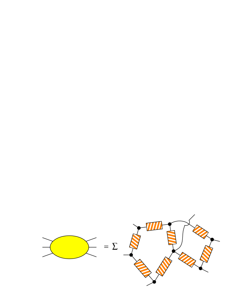
Figure 3: Example of a diagram with dressed propagator insertions

Our procedure for rearranging Feynman diagrams begins with dressing all propagators. We use the notation illustrated in Fig. 2. Thus, from now on, all propagators in a diagram are assumed to include the one-particle irreducible 2-point diagrams, which form a geometric series. A generic diagram will look as illustrated in Fig. 3.

Next, we consider all one-particle irreducuble 3-point diagrams. They can also be added, once and for all, to all bare 3-point vertices, to for m the so-called dressed 3-point vertices. Similarly, we can collect all subdiagrams needed to turn all 4-vertices into dressed 4-vertices, see Fig. 4. It is important that diagrams, where the propagators and vertices are replaced by dressed ones, themselves should not contain any other subgraphs with three or four external lines.

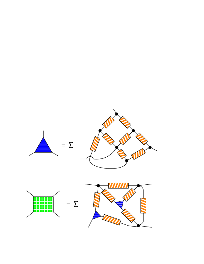
Figure 4: The dressed 3-point vertices formed from irrdeucible subdiagrams, and the dressed 4-point vertices from irrdeucible 4-point diagrams

A generic diagram then looks as in Fig. 5.

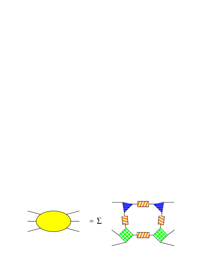
Figure 5: Diagrams with more than 4 external lines are built exclusively of dressed propagators, dressed 3-point vertices and dressed 4-point vertices

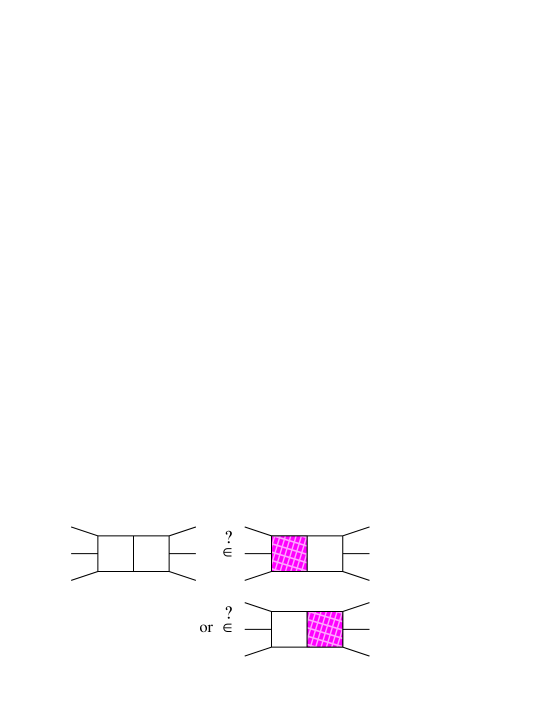
Figure 6: Ambiguity for irreducible 5-point vertices: the diagram indicated has six external lines and can be written in two ways using an irreducible 5-vertex. It would be counted twice, which is incorrect unless further correction procedures are introduced

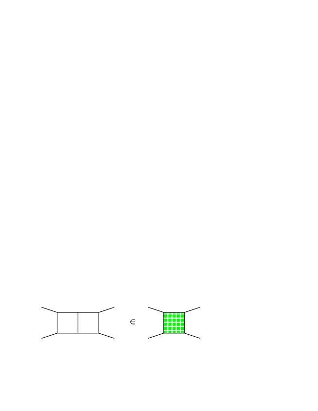
Figure 7: Subgraphs with 4 external lines do not lead to counting errors. The diagram depicted here contributes just once to the irreducble dressed 4-vertex

It is important to check here that rearranging diagrams using this prescription does not lead to omissions of any diagrams or to overcounting of diagrams. Indeed, if we were to continue the procedure towards irreducible diagrams with five external lines, overcounting would occur. This is illustrated in Fig. 6. Such an ambiguity cannot occur in the case of 4-vertices; cf. Fig. 7. The diagram of this Figure is counted correctly as a single contribution to the dressed 4-vertices.

We conclude from this section that all diagrams with five or more external lines can be seen to be built up in an unambiguous way from irreducible dressed propagators, 3-point functions and 4=point functions. These dressed diagrams themselves should not contain any irreducible subgraph with less than five external lines. Consequently, the integrations over any of the momenta in these dressed diagrams do not lead to any ultraviolet divergence. In particular, there are no overlapping ultraviolet divergences.

However, the dressed 2-, 3- and 4-point functions themselves cannot be reduced to convergent integrals along such lines; they themselves still seem to be built out of bare propagators and vertices. They will be considered in the next sections.

2 The Ariadne Procedure

The dressed 2-, 3- and 4-point vertices may be divergent, but if we introduce subtractions, more convergent expressions may arise. We claim that, if a divergent, irreducible diagram with $n<5$ external lines is considered, then we can take the difference between that diagram and the same diagram at some different values of its external momenta, and rewrite that as a new irreducible Feynman diagram with $n+1$ external lines, whose degree of convergence is improved by at least one power of $k$.

In order to introduce unambiguous rules for these difference diagrams, we need the notion of a guiding path inside a diagram. A guiding path is a sequence of propagators inside a diagram that form a single uninterrupted line from one external line to another, see Fig. 8. If an external line is a fermion, such as in QED, we can use this fermion as a guiding path. In $U(N)$ (gauge) theories, we can often use index lines as guiding paths, provided that not all index lines lead from one external line back to the same one; since such diagrams do not contribute in $SU(N)$ theories (fields in the adjoint representation are traceless), index lines are assured to be useful in these theories. However, also in $SO(N)$ theories, index lines cannot run from one external line back to the same line, since here also the adjoint representation is traceless. This means that also $U(1)$ theories can sometimes be handled. If, however, an external line has two (or more) units of $U(1)$ charge, it means that it has two index lines in terms of which the representation is symmetric, hence not traceless. In that case, we have to use some other guiding line. In the electro-weak case, this appears to be possible: all our bosonic fields have several quantum numbers, so that we do not have to resort on the unreliable $U(1)$ indices.

Thus, it seems that in most cases of interest one can find a guiding path. This will be referred to as the Ariadne principle. It is the one restriction that we will assume, besides the more familiar restriction that our theory should not contain any chiral anomalies[3] (more about the anomalies later).

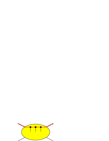
Figure 8: The introduction of a guiding path (dotted line)

Consider the sequence of (bare) propagators $P(k_{i})$ and (bare) vertices $V(k_{i})$ along a guiding path that leads from an external line with momentum $k_{0}$ to another line with momentum $k_{N}$.

$$F(k_{0},\,k_{N})=V_{1}(k_{1})P_{1}(k_{1})\,\cdots\,P(k_{N-1})V_{N}(k_{N})\,;$$ (2.1)

Here, and $k_{i}$ is the momentum in the $i^{\mathrm{th}}$ propagator or vertex, $i$ running from 1 to $N$. Now substitute all these momenta by the same values plus an additional, fixed, momentum $q$, and compute the difference between these two amplitudes:

$$F(k_{0}+q,\,k_{N}+q)-F(k_{0},\,k_{N})\ =\sum_{i}\Bigg{\{}V_{1}(k_{1})\cdots P_{i-1}(k_{i-1})$$ (2.2)

$$\bigg{(}\Big{(}V_{i}(k_{i}+q)-V_{i}(k_{i})\Big{)}P_{i}(k_{i}+q)+V_{i}(k_{i})\Big{(}P_{i}(k_{i}+q)-P_{i}(k_{i})\Big{)}\bigg{)}$$ (2.3)

$$V_{i+1}(k_{i+1}+q)\,P_{i+1}(k_{i+1}+q)\,\cdots\,V_{N}(k_{N}+q)\Bigg{\}}\,.$$ (2.4)

We see that this expression contains bare propagators and vertices that again form dressed propagators and vertices when summed. In particular, parts of this expression refer to the difference between two dressed propagators, which obey

$$P^{\mathrm{\,dr}}(k) = \Big{(}k^{2}+m^{2}-\Gamma(k)-i\varepsilon\Big{)}^{-1}\quad;$$

$$P^{\mathrm{\,dr}}(k+q)-P^{\mathrm{\,dr}}(k) = P^{\mathrm{\,dr}}(k)\,\Big{[}\Gamma(k+q)-\Gamma(k)-(k+q)^{2}+k^{2}\Big{]}\,P^{\mathrm{\,dr}}(k+q)\,.\ {}$$ (2.5)

Writing

$$k^{2}-(k+q)^{2}=-q_{\mu}(2k^{\mu}+q^{\mu})\ ;\qquad\Gamma(k+q)-\Gamma(k)=q_{\mu}\Gamma_{1}^{\mu}(k,q)\ ,$$ (2.6)

we see that the expression between square brackets here can be regarded as an effective three-point diagram $\Gamma_{1}^{\mu}$, multiplied with a factor $q_{\mu}$. Eq. (2.5) is depicted diagrammatically in Fig. 9.

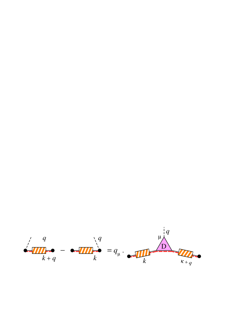
Figure 9: Difference between two dressed propagators in diagrammatic notation

3 Integrating the equations. Conclusion

Similarly, we can handle the difference between three-point diagrams, $V^{[3]}(k+q)-V^{[3]}(k)$, at different external momenta as four-point diagrams, see Fig. 10. The difference between two four-point diagrams is a sum of convergent diagrams, see Fig. 11. The difference equations used here can be used either for the original irreducible diagrams for the theory or for the diagrams obtained after a previous differenciation. In all cases, the irreducible diagrams of five or more external lines only contain convergent expressions. As far as the ultra-violet divergences is concerned, the situation is the same as if we had differentiated with respect to the momenta rather than taking finite differences (i.e., if $q$ had been taken infinitesimal. A disadvantage of infinitesimal $q$, however, is the emergence of higher order poles and the associated infra-red divergences in the propagators. Our difference procedure avoids infra-red divergences.

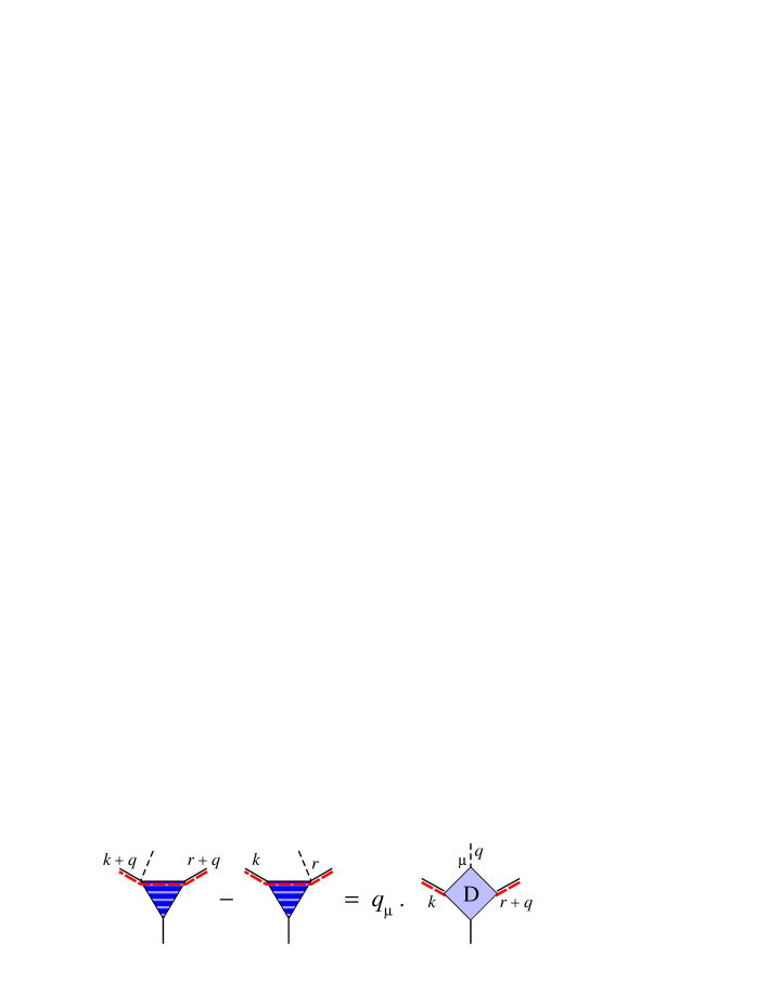
Figure 10: The difference between the 3-point functions at different values of the external momenta is a four-point diagram

Fig. 11, whose equation reads as:

$$V^{[4]}(k+q)-V^{[4]}(k)=q_{\mu}\sum_{i}V^{\mu\,[5]}_{i}(k,q,\cdots)\ ,$$ (3.1)

where $V_{i}^{\mu[5]}$ do not contain any divergences, in many respects is to be regarded as a renormalization group equation. Since $V_{i}^{\mu[5]}$ are all linearly (or better) convergent, the equation can be symbolized as

$${d\over dk}\Gamma^{[4]}(k)={1\over k}\beta(\Gamma^{[4]})(k)\,,$$ (3.2)

the r.h.s. being essentially a beta function. The difference equations for the 2- and 3-point functions, in short-hand, are

$$\Gamma^{[2]}(k+q)-\Gamma^{[2]}(k) = q^{\mu}\,k\,(D\Gamma)^{[3]}_{\mu}(k,q)\ ,$$ (3.3)

$$V^{[3]}(k+q)-V^{[3]}(k) = q^{\mu}\,(DV)^{[4]}_{\mu}(k,q)\ ,$$ (3.4)

where we explicitly indicated the $k$-dependence apart from logarithms. Thus, we see that Eqs. (3.3) and (3.4) converge in the infrared when integrated, whereas (3.2) has the infra-red structure of the renormalization group.[4]

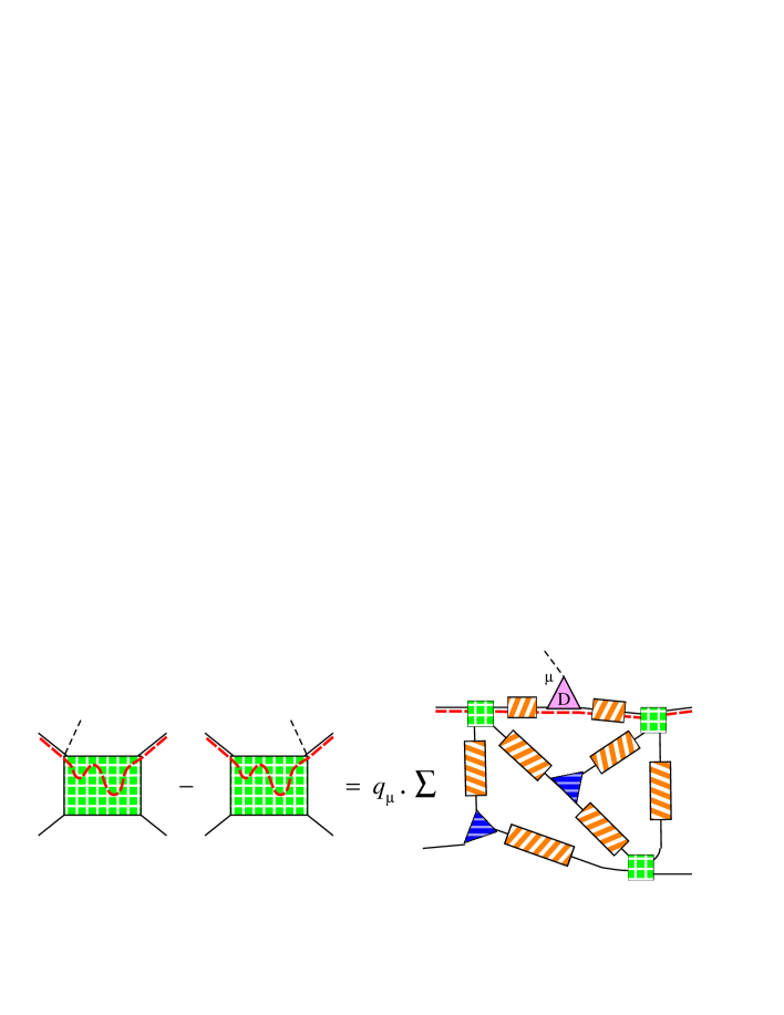
Figure 11: The difference between the 4-point functions at different values of the external momenta is a sum of convergent diagrams

Our set of equations appears to be particularly elegant because no direct reference is made to the bare Lagrangian of the theory! All bare coupling parameters are generated by the integration constants when integrating these difference equations.

Thus, Quantum Field Theory has been recast into a self-consistent set of equations, which can be integrated to obtain the desired amplitudes. The four-point amplitudes – more precisely, the canonically dimensionless irreducible $n$-point functions – follow from solving the renormalization group equation Eq. (3.1). The required integration constant(s) replace the original free parameters of the theory.

A difficulty may arise from the fact that the ‘guiding lines’ may be chosen in many alternative ways. Indeed, it is in integrating the equations that one might encounter anomalies[3]: the integration constants cannot be reconciled with all symmetries of the theory.

Also, the lower irreducible Green functions may generate integration constants, which would correspond to dimensionful parameters of the theory. The usual questions concerning “naturalness” are not affected by our procedure; if the integration constants lead to small amplitudes in the far infra-red, this may be considered as ‘unnatural’, but there is no objection to that from a purely mathematical point of view.

Another fundamental difficulty not addressed by our procedure is the divergence of the perturbative expansion for the diagrams in the r.h.s. of Eq. (3.1), depicted in Fig. 11. In general, such expansions diverge factorially. In the planar $N\rightarrow\infty$ limit, the number of diagrams increases by calculable power laws, but individual diagrams may grow factorially, so that there still is no guarantee for a finite radius of convergence.[2] In practice, it seems to be not unreasonable to simply cut the series off at some given order.

References

- [1] C. Itzykson and J.-B. Zuber, Quantum Field Theory, McGraw-Hill 1985; ISBN 0-07-032071-3; 0-07-066353-X.
- [2] G, ’t Hooft, Planar diagram field theories, in Progrss in Gauge Field Theory, NATO Adv. Study Inst. Series, eds. G. ’t Hooft et al., Plenum, 1984, 271, reprinted in G. ’t Hooft, Under the Spell of the Gauge principle, World Scientific, 1994, p. 378. See also: Nucl. Phys. B 72 (1974) 461.
- [3] S.L. Adler, Phys. Rev. 177 (1969) 2426; J.S. Bell and R. Jackiw, Nuovo Cim. 60A (1969) 47; S.L. Adler and W.A. Bardeen, Phys. Rev. 182 (1969) 1517; W.A. Bardeen, Phys. Rev. 184 (1969) 1848.
- [4] C.G. Callan, Phys. Rev. D2 (1970) 1541; K. Symanzik, Commun. Math. Phys. 16 (1970) 48; ibid. 18 (1970) 227.