MPP-2004-43

May 2004

Structure functions of $2d$ integrable asymptotically free models

Janos Balog

Research Institute for Particle and Nuclear Physics

1525 Budapest 114, Pf. 49, Hungary

Peter Weisz

Max-Planck-Institut für Physik

Föhringer Ring 6, D-80805 München, Germany

Abstract

We investigate structure functions in the 2–dimensional (asymptotically free) non–linear O$(n)\,\,\sigma$–models using the non–perturbative S–matrix bootstrap program. In particular the exact small (Bjorken) $x$ behavior is exhibited; the structure is rather universal and is probably the same in a wide class of (integrable) asymptotically free models. Structurally similar universal formulae may also hold for the small $x$ behavior of QCD in 4–dimensions. Structure functions in the special case of the $n=3$ model are accurately computed over the whole $x$ range for $-q^{2}/M^{2}<10^{5}$, and some moments are compared with results from renormalized perturbation theory. Some remarks concerning the structure functions in the $1/n$ approximation are also made.

1 Introduction

Structure functions describing scattering of electrons and neutrinos off nucleon targets are well measured and give us insight into the structure of the nucleons [?,?,?,?]. At high $-q^{2}$ and intermediate Bjorken $x$ the parton model and DGLAP equations [?,?] give a good description. At smaller $x$ the DLGAP equations are considered to break down and BFKL–type [?] equations take over, here the structure function $F_{2}\sim x^{-\nu(-q^{2})}$ with $\nu(-q^{2})>0$. A value of $\nu(0)>0$ would however (seem to) violate the Froissart bound. Recently saturation models, such as the so–called color glass model [?,?] predict the true asymptotic behavior to be $F_{2}\sim\ln^{p}x\,,$ with $p=1$ or 2.

The QCD literature on small $x$ physics is vast and rather involved [?,?]. One certain aspect is that a description of the asymptotically small $x$ region requires some crucial non–perturbative input. The most systematic non–perturbative methods for QCD, using the lattice regularization, are able to give non–perturbative information on the moments of the structure functions via the OPE [?,?], however they are not applicable to yield information on the asymptotically small $x$ behavior.

In this paper we study structure functions in asymptotically free integrable models in two dimensions. Despite the fact that there are no transverse directions, the structure functions have a rather rich and non–trivial behavior with many features reminiscent of the structure functions in QCD. Here we will concentrate on results obtained for O$(n)$ sigma models. In particular we have derived the exact small $x$ behavior in these models. The result has a rather universal model–independent structure, being independent of $n$ and holding for a large class of operator probes. One is tempted to speculate a similar qualitative structure to hold in QCD.

2 Sigma model 2–point functions

The O$(n)$ $\sigma$–model in $2d$ formally described by the Lagrangian

$${\cal L}=\frac{1}{2g_{0}^{2}}\sum_{a=1}^{n}\partial_{\mu}S^{a}\partial^{\mu}S^{a}\,,\,\,\,\,\,\,\,\,\sum_{a=1}^{n}S^{a}S^{a}=1\,,$$ (2.1)

is perturbatively asymptotically free for $n\geq 3$. A special property is that these models have an infinite number of local [?] and non–local [?] classical conservation laws which survive quantization. At the quantum level they imply absence of particle production. Assuming the spectrum to consist of one stable O$(n)$–vector multiplet of mass $M$, the S–matrix has been proposed long ago by the Zamolodchikovs [?]. Form factors of local operators can be computed using general principles [?]. The S–matrix bootstrap program for the construction of correlation functions involves summing the contributions over all intermediate states [?]. The possible equivalence of this construction to the continuum limit of the lattice regularized theory has been investigated in ref. [?]. In papers of one of the present authors (J.B) and M. Niedermaier [?] 2–point functions of various operators were computed, including those of the O($n$) current $J_{\mu}^{cd}$ and spin–field operators $\Phi^{a}$. We give their definitions here because they will be needed later to state our result on the small $x$ behavior:

$$\langle 0|T\,J^{cd}_{\mu}(x)J^{ef}_{\nu}(y)|0\rangle=$$

$$-i\left(\delta^{ce}\delta^{df}-\delta^{cf}\delta^{de}\right)\int\frac{{\rm d}^{2}q}{(2\pi)^{2}}{\rm e}^{-iq(x-y)}\left(q_{\mu}q_{\nu}-q^{2}\eta_{\mu\nu}\right)I_{1}(-q^{2}-i\epsilon)\,,$$ (2.2)

valid up to contact terms and

$$\langle 0|T\Phi^{a}(x)\Phi^{b}(y)|0\rangle=-i\delta^{ab}\Lambda_{n}^{2}\int\frac{{\rm d}^{2}q}{(2\pi)^{2}}{\rm e}^{-iq(x-y)}I_{0}(-q^{2}-i\epsilon)\,,$$ (2.3)

where the normalization factor $\Lambda_{n}$ is chosen (for later convenience):

$$\Lambda_{3}=\frac{2}{\sqrt{\pi}}\,,\,\,\,\,\,\Lambda_{n}=1\,\,\,\,\,n>3\,.$$ (2.4)

To complete the definitions we must supplement the operator normalizations. The currents have a normalization fixed by requiring their spatial integrals to yield the correct charges (cf Eq. (4.41)), and our field normalization is fixed by requiring

$$\langle 0|\Phi^{a}(0)|b,\theta\rangle=\delta^{ab}$$ (2.5)

for one particle states with momentum $p_{1}=M\sinh\theta$, with state normalization

$$\langle a,\theta^{\prime}|b,\theta\rangle=4\pi\delta^{ab}\delta(\theta^{\prime}-\theta)\,.$$ (2.6)

The studies of these 2–point functions (in the case $n=3$) [?] presently constitute the best evidence for the existence of a non–perturbative construction of a model with asymptotic freedom.

3 Sigma model structure functions

The $\sigma$–model analogue of the central object in deep inelastic scattering is

$$W^{ab;cdef}_{\mu\nu}(p,q)={1\over 4\pi}\int{\rm d}^{2}xe^{iqx}\langle a,p|\Bigl{[}J_{\mu}^{cd}(x),J_{\nu}^{ef}(0)\Bigr{]}|b,p\rangle\,.$$ (3.7)

We define the usual DIS kinematic variables

$$\nu=pq/M\,,\,\,\,\,\,\,\,x=-q^{2}/(2M\nu)\,,\,\,\,\,\,\,\,W^{2}=(p+q)^{2}\,.$$ (3.8)

In the relevant kinematic domain $q^{2}<0,W\geq M$ i.e. $0\leq x\leq 1$ we have

$$W^{ab;cdef}_{\mu\nu}(p,q)=\pi\sum_{r}\langle a,p|J_{\mu}^{cd}(0)|r\rangle\langle r|J_{\nu}^{ef}(0)|b,p\rangle\delta^{(2)}(p+q-P_{r})\,,$$ (3.9)

where the sum is over the complete set of $r$–particle (“in” or “out”) states. Using Lorentz and O$(n)$ invariance we have

$$W^{ab;cdef}_{\mu\nu}(p,q)=\left(\eta_{\mu\nu}-\frac{q_{\mu}q_{\nu}}{q^{2}}\right)\sum_{l=0}^{2}w_{l}(q^{2},x)R_{l}^{ab;cdef}\,,$$ (3.10)

with projectors $R_{l}$ corresponding to the 3 invariant $t$–channel “isospins” given by

$$R_{0}^{ab;cdef} = \frac{1}{n}\delta^{ab}(\delta^{ce}\delta^{df}-\delta^{cf}\delta^{de})\,,$$ (3.11)

$$R_{1}^{ab;cdef} = \frac{1}{2}(\delta^{ac}\delta^{be}-\delta^{bc}\delta^{ae})\delta^{df}-(c\leftrightarrow d)-(e\leftrightarrow f)+(c\leftrightarrow d\,,e\leftrightarrow f),$$ (3.12)

$$R_{2}^{ab;cdef} = -\frac{1}{2}\Bigl{\{}(\delta^{ac}\delta^{be}+\delta^{bc}\delta^{ae})\delta^{df}-(c\leftrightarrow d)-(e\leftrightarrow f)+(c\leftrightarrow d\,,e\leftrightarrow f)\Bigr{\}}$$ (3.13)

$$+\frac{2}{n}\delta^{ab}(\delta^{ce}\delta^{df}-\delta^{cf}\delta^{de})\,.$$

Note in 2 dimensions there is only one structure function for each isospin channel, since there is only one (conserved symmetric) tensor involving two momenta; one has e.g. ( for $p^{2}=M^{2}$)

$$\Bigl{(}p_{\mu}-{M\nu q_{\mu}\over q^{2}}\Bigr{)}\Bigl{(}p_{\nu}-{M\nu q_{\nu}\over q^{2}}\Bigr{)}=\frac{M^{2}(\nu^{2}-q^{2})}{(q^{2})^{2}}\left(q_{\mu}q_{\nu}-\eta_{\mu\nu}q^{2}\right)\,.$$ (3.14)

Although in QCD structure functions for operators not associated with physical sources have so far not been studied, we also introduce, for reasons which will soon become apparent, the field structure functions through

$$\Sigma^{ab;cd}(p,q) = -\pi q^{2}\sum_{r}\langle a,p|\Phi^{c}(0)|r\rangle\langle r|\Phi^{d}(0)|b,p\rangle\delta^{(2)}(p+q-P_{r})$$ (3.15)

$$= \Lambda_{n}^{2}\sum_{l=0}^{2}{\widetilde{w}}_{l}(q^{2},x)P_{l}^{ab;cd}\,,$$ (3.16)

with $t$–channel projectors $P_{l}$ for the vector representation given by

$$P_{0}^{ab;cd} = \frac{1}{n}\delta^{ab}\delta^{cd}\,,$$ (3.17)

$$P_{1}^{ab;cd} = \frac{1}{2}\Bigl{(}\delta^{ac}\delta^{bd}-\delta^{bc}\delta^{ad}\Bigr{)}\,,$$ (3.18)

$$P_{2}^{ab;cd} = \frac{1}{2}\Bigl{(}\delta^{ac}\delta^{bd}+\delta^{bc}\delta^{ad}\Bigr{)}-\frac{1}{n}\delta^{ab}\delta^{cd}\,.$$ (3.19)

The current operators connect only states with an even number of particles to the vacuum and the field operators only states with and odd number:

$$w_{l}(q^{2},x)=\sum_{r\,\,{\rm odd}}w_{l}^{(r)}(q^{2},x)\,,\,\,\,\,\,\,\,\,{\widetilde{w}}_{l}(q^{2},x)=\sum_{r\,\,{\rm even}}w_{l}^{(r)}(q^{2},x)\,.$$ (3.20)

The wonderful feature of integrable models is that one knows many explicit properties concerning the form factors appearing in the expressions. These are encapsulated in the Smirnov axioms [?], and using these one can derive the previously announced exact asymptotic small $x$ behavior of the structure functions:

$$w_{l}(q^{2},x)\sim\frac{1}{x\ln^{2}x}\frac{2\pi T_{l}}{(n-2)^{2}}A_{1}(-q^{2})\,,$$ (3.21)

$${\widetilde{w}}_{l}(q^{2},x)\sim\frac{1}{x\ln^{2}x}\frac{2\pi V_{l}}{(n-2)^{2}}A_{0}(-q^{2})\,,$$ (3.22)

where the functions $A_{s}$ are the “Adler functions” defined from the vacuum 2–point functions (2.2),(2.3) by

$$A_{s}(z)=-z^{2}\frac{\partial}{\partial z}I_{s}(z)\,,\,\,\,\,\,s=0,1\,.$$ (3.23)

The constants appearing in (3.21),(3.22) are characteristic of the O$(n)$ representations (vector $V$ and anti–symmetric tensor $T$) of the corresponding operators:

$$V_{0}=2(n-1)\,,\,\,\,\,\,V_{1}=V_{2}=n-2\,,$$ (3.24)

$$T_{0}=4(n-2)\,,\,\,\,\,\,T_{1}=n-2\,,\,\,\,\,T_{2}=4-n\,.$$ (3.25)

The explicit proof of these relations will be presented in a forthcoming more detailed publication [?]. In this letter we would like to concentrate on general features. Firstly we note that the structure of the asymptotic small $x$ behavior is independent of the operator, independent of $n$, and independent of the channel. Further since the results were obtained from rather general principles, we think that they are valid for a large class of integrable asymptotically free models. Indeed we have checked that the same behavior holds in the leading orders of the $1/n$ expansion in the Gross–Neveu model [?].

In the derivation of (3.21),(3.22) it appears that the $1/\ln^{2}x$ behavior is related to the high energy behavior of the scattering amplitudes; this is similar to the association of the proposed $\ln^{p}x$ in QCD with the asymptotic behavior of total cross sections (related to the forward scattering amplitude through the optical theorem).

The question is what can one learn for QCD; is the small $x$ behavior there also given by a structural formula factorizing a part characteristic to the target and a part described by the vacuum 2–point function? Unfortunately so far we have not succeeded to derive such a general result. As a first guess we have looked at the ratio of the structure function $F_{2}$ to the (electro–magnetic) Adler function $D$ in QCD, with HERA data at some of the lowest $x$ values published so far [?], and the Adler function taken from ref. [?]. The result is presented in Fig. 1; there is no sign that the ratio is becoming independent of $-q^{2}$ as $x$ decreases. However from such comparisons one should be cautious to draw conclusions concerning the asymptotic behavior, because at these values of $x$ the situation is qualitatively similar (only the slope is different) for the ratio $xw_{0}(q^{2},x)/A_{1}(-q^{2})$ in the O(3) $\sigma$–model, which is also plotted in the same figure. In this model one would have to go to much smaller values of $x$. The question remains for QCD, at which value of $x$ (for a given $-q^{2}$ range) does the true asymptotic behavior set in?

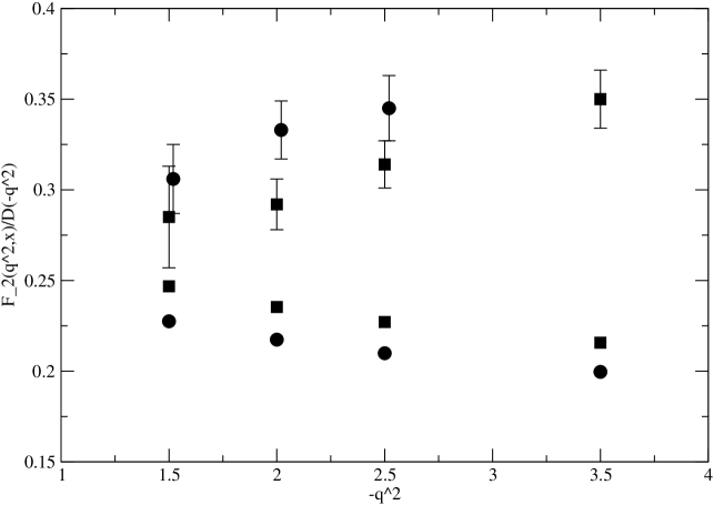
Figure 1: $F_{2}(q^{2},x)/D(-q^{2})$ for $x=5\cdot 10^{-5}$ (circles with error bars) and $x=8\cdot 10^{-5}$ (squares with error bars), for various values of $-q^{2}$ (in ${\rm GeV}^{2}$). Symbols without error bars are values of $xw_{0}(q^{2},x)/A_{1}(-q^{2})$ in the O(3) $\sigma$–model at the same values of $x$ (here the abscissa denotes values of $-q^{2}/M^{2}$).

The QCD structure functions in the range of small $x$ between $10^{-5}$ and $10^{-2}$ are fitted quite well with a “Lipatov form” $A(-q^{2})x^{-\nu(-q^{2})}$. As an exercise we have made least–square fits of $xw_{0}(q^{2},x)$ (for O(3)) with such a form and observed that in the regime $10^{-5}\leq x\leq 10^{-3}$ such fits with $\nu(-q^{2})=-0.192,\,-0.167,\,-0.151$ for $-q^{2}/M^{2}=1,10,100$ respectively, describe the data better than simplest fits of the form $C(-q^{2})/\ln^{2}x$ incorporating the known asymptotic small $x$ behavior.

3.1 $1/n$ expansion

The data obtained for O(3) used above and in subsequent sections require a considerable amount of computation. For this reason we include here a short discussion of structure functions in leading order of the $1/n$ expansion, where many qualitative results are rather similar to $n=3$ but where relatively simple analytic formulae are available. The easiest case is the leading order of the spin structure functions in the isospin 1,2 channels because they are given by the imaginary part of the propagator of the “auxiliary field”:

$${\widetilde{w}}_{l}(q^{2},x) = \frac{1}{n}\theta(W-2M)4\pi\frac{-q^{2}M^{2}}{(-q^{2}+M^{2})^{2}}\frac{\sinh\theta}{\theta^{2}+\pi^{2}}+{\rm O}(1/n^{2})\,,$$ (3.26)

$${\rm for}\,\,\,W^{2}=4M^{2}\cosh^{2}\frac{\theta}{2}\,,\,\,\,l=1,2\,.$$

Apart from suggesting that the limits $n\to\infty$ and $x\to 0$ commute, this simple function already illustrates many rather general features of the structure functions in this model. Firstly that the onset of the limit $x\to 0$ is not uniform in $-q^{2}$. In the Bj–limit $-q^{2}\to\infty\,,\,\,\,\,x\,\,{\rm fixed}$ we have

$${\widetilde{w}}_{l}(q^{2},x)\sim\frac{1}{n}\frac{2\pi(1-x)}{x\ln^{2}(-q^{2}/M^{2})}\,,\,\,\,\,\,l=1,2.$$ (3.27)

Secondly the limit $x\to 0$ for fixed $q^{2}$ is approached extremely slowly e.g. for $-q^{2}/M^{2}=1\,,\,\,{\widetilde{w}}_{l}/({\widetilde{w}}_{l})_{\rm asympt}=0.93$ for $x=10^{-5}$, while for $-q^{2}/M^{2}=100$ we have e.g. ${\widetilde{w}}_{l}/({\widetilde{w}}_{l})_{\rm asympt}=0.49,0.59$ for $x=10^{-5},10^{-7}$ respectively.

We remark that the leading order (in $1/n$) isospin 0 (field) structure function involves another (box) diagram which is also easily evaluated. One can show that the small $x$ behavior is as predicted by the general formula (3.22). The leading $1/n$ diagram contributing to the current structure functions is just a 1–particle exchange and thus only contributes a term $\propto\delta(1-x)$. We have computed the next–to–leading orders for the $l=1,2$ channels and again confirm the predicted behavior.

3.2 The case $n=3$

So far we have concentrated on the small $x$ region; in the following we extend our description of the structure functions to the whole range of $x$. We will do this for the case $n=3$ which is rather special for various reasons. For our studies in the S–matrix bootstrap approach it is important that it is the model for which the $r$–particle form factors can most easily be obtained explicitly. Moreover the spin and current 2–point functions exhibit in this case very similar features and there are miraculous scaling relations [?] which relate them . There are well defined recursive procedures for computing the form factors, the only practical limitation being that they become very involved. So far the record we have achieved is the 7–particle form factor of the spin field [?]; already its algebraic expression in MAPLE involves many megabytes of storage. Fortunately for the structure functions we only require sums over bilinear factors of the form factors which are computationally more manageable.

Just as for the 2–point functions [?] we find that for a fixed $-q^{2}$ only states with a limited number of particles contribute significantly. To appreciate this better we consider the sum of the field and current structure functions, which is a rather peculiar thing to do in general, but which is in fact rather natural in the special case $n=3$. Figs. 2 and 3 illustrate how the structure function $x(w_{0}+{\widetilde{w}}_{0})$ is built up from states with increasing particle number for the cases $-q^{2}/M^{2}=10^{2}$ and $-q^{2}/M^{2}=10^{4}$ respectively. We see that the higher states contribute very little and that we obtain nearly exact values for the structure functions for all values of $-q^{2}/M^{2}<10^{5}$ by including only intermediate states with $\leq 5$ particles for the current and $\leq 6$ particles for the spin field.

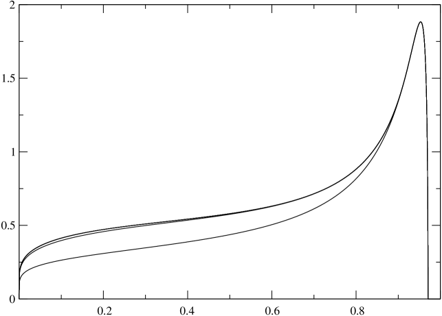
Figure 2: Approximations to $x(w_{0}+{\widetilde{w}}_{0})$ as functions of $0<x<1$ for $-q^{2}/M^{2}=100$. Curves correspond to sums up to and including $2,3,4,5,6$–particle intermediate states. The last 3 curves are indistinguishable on this scale.

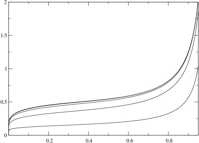
Figure 3: Approximations to $x(w_{0}+{\widetilde{w}}_{0})$ functions of $0<x\leq 0.95$ for $-q^{2}/M^{2}=10^{4}$. Curves correspond to sums up to and including 2,3,4,5,6–particle states.

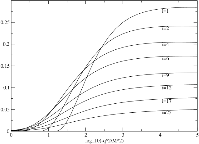
Figure 4: $xw_{0}(q^{2},x)$ for various values of $x=10^{-i/5}$.

In Fig. 4 we plot $xw_{0}(q^{2},x)$ as a function of ${\rm log}_{10}(-q^{2}/M^{2})$, for a selection of $x$–values . The function increases as $-q^{2}$ increases for all values of $x$ in this range.

3.3 Threshold behavior

Note that in Fig. 3 we have cut off the plot at $x=0.95$. This is because near $x=1$ the function develops a big bump with a peak $\sim 70$ which, if included in the same plot, would obscure the features we wanted to show there. The behavior of the $\sigma$–model structure functions near $x=1$ is indeed rather involved. For a fixed $-q^{2}$ the contribution to the structure function from the $r$–particle state $w^{(r)}$ vanishes for $x$ greater than some threshold value

$$x_{r}(-q^{2})=\left[1-(r^{2}-1)M^{2}/q^{2}\right]^{-1}\,.$$ (3.28)

The big bump in $x(w_{0}+{\widetilde{w}}_{0})$ referred to above is at this value of $-q^{2}/M^{2}=10^{4}$ practically entirely due to the $2$–particle contribution. For this contribution:

$$w^{(2)}_{l} \sim E_{l}(q^{2})\sqrt{x_{2}(-q^{2})-x}\,,\,\,\,x\to x_{2}\,,\,\,\,-q^{2}\,\,\,\,{\rm fixed}\,,$$ (3.29)

$$w^{(2)}_{l} \sim F_{l}(x)/\ln^{2}(-q^{2}/M^{2})\,,\,\,\,-q^{2}\to\infty\,,\,\,\,x\,\,\,\,{\rm fixed}\,,$$ (3.30)

where $E_{l},F_{l}$ are some (known) functions. The bump arises because $F_{l}$ is quite singular near threshold, $F_{l}\sim[(1-x)\ln^{2}(1-x)]^{-1}$. The analytic behavior as $x\to x_{2}$ sets in only extremely close to threshold e.g for $-q^{2}/M^{2}=10^{4}$ the position of the peak of the bump is at $x=0.99954$ whereas the function vanishes at $x_{2}=0.99970$. At $-q^{2}/M^{2}=10^{4}$ the 3–particle contribution also has a bump but it is less pronounced; (peak value $\sim 2.5$ at $x\sim 0.9953$). We conjecture that the threshold behavior of $w_{0}^{(r)}$ in the O(3) model is $(x_{r}-x)^{(r^{2}-3)/2}$.

One can also study the threshold behavior in the $n\to\infty$ limit. Here we find that in the leading order ${\widetilde{w}}_{l}\sim\sqrt{x_{2}(-q^{2})-x}$ for $l=1,2$ but ${\widetilde{w}}_{0}\sim 1/\sqrt{x_{2}(-q^{2})-x}$. We caution however that the limits $n\to\infty$ and $x\to$ threshold may not commute.

The characteristic enhanced near–threshold features in this model probably have no counterpart in QCD. For QCD the behavior of the structure functions in the $x\sim 1$ region is surely also complicated. But there the effects might be quite suppressed for large $-q^{2}$ since, if we model the behavior in this region by the contribution of resonances, their electromagnetic form factors are thought to fall very quickly (as powers) in $-q^{2}$ similarly to that of the proton.

4 Partons, OPE and moments

4.1 Parton model

In the O$(n)\,\,\sigma$–models there does not seem to be a simple parton picture. This is even so for the case $n=3$ where the model is equivalent to the $\rm\kern 2.5pt\vrule height=6.02773pt,depth=-0.51663pt,width=0.59998pt\kern-3.09998ptC{\rm P}^{1}$ model. For although this model is formulated in terms of a complex doublet of fields which are analogous to quarks in that they are confined, it seems that they do not play a rôle more similar to partons than the elementary bare spin fields in the original formulation . The question is related to that of understanding what are (if any) the “ultra–particles” in the sense of Buchholz and Verch [?], or to the associated question as to whether the $\sigma$–models have an underlying conformal field theory.

Although an intuitive parton description with suggestive DGLAP equations

$$q^{2}\frac{\partial}{\partial q^{2}}w_{l}(q^{2},x)=\int_{x}^{1}\frac{{\rm d}y}{y}p_{l}(x/y,q^{2})w_{l}(q^{2},y)\,,$$ (4.31)

(where $p_{l}(z,q^{2})$ would be the corresponding splitting functions) is still missing in these models, we still have the machinery of the operator product expansion (OPE) which we apply in the following.

4.2 Moments

A class of interesting quantities are the moments of the structure functions:

$$M_{l;N}(q^{2}) = \int_{0}^{1}{\rm d}xx^{N-1}w_{l}(q^{2},x)=\sum_{r={\rm odd}}M_{l;N}^{(r)}(q^{2})\,,$$ (4.32)

$${\widetilde{M}}_{l;N}(q^{2}) = \int_{0}^{1}{\rm d}xx^{N-1}{\widetilde{w}}_{l}(q^{2},x)=\sum_{r={\rm even}}M_{l;N}^{(r)}(q^{2})\,,$$ (4.33)

where $M_{l;N}^{(r)}(q^{2})$ denote the contributions from $r$–particle states

$$M_{l;N}^{(r)}(q^{2})=\int_{0}^{1}{\rm d}xx^{N-1}w_{l}^{(r)}(q^{2},x)\,.$$ (4.34)

As in QCD the moments satisfy renormalization group equations from which one can determine their leading behavior as $-q^{2}\to\infty$. These are derived by considering the OPE for the current–current and field–field products and explicitly treating the terms involving the operators of highest (zero) twist . The general analysis is rather involved because the classification of lowest twist operators turns out to be more complicated than in QCD because the elementary field is dimensionless . Our analysis extends that initiated e.g. in refs.[?], [?]. Here we just quote some results and defer the derivations to ref. [?].

For the current ($N$ even) moments in the isospin 0 channel we have

$$M_{0;N}(q^{2})=W_{0;N}\,\frac{n-2}{2(n-1)}\,\left\{1+\frac{1}{n-2}\lambda(q^{2})+{\rm O}\left(\lambda^{2}\right)\right\}\,,\,\,\,N\geq 2\,,$$ (4.35)

where $\lambda(q^{2})$ is an effective running coupling function defined through

$$\frac{1}{\lambda(q^{2})}+\frac{1}{n-2}\ln\lambda(q^{2})=\ln\frac{\sqrt{-q^{2}}}{\Lambda_{\rm\overline{MS\kern-0.98pt}\kern 0.98pt}}\,,$$ (4.36)

and the $W_{0;N}$ are renormalization group invariant, non-perturbative constants, corresponding to the matrix elements of spin $N$ operators. In the $N=2$ case this is the energy–momentum tensor operator $T_{\mu\nu}$ for which we know the constant explicitly

$$\langle a,\theta|T_{++}(0)|b,\theta\rangle=\frac{1}{4}W_{0;2}M^{2}{\rm e}^{2\theta}\delta^{ab}\,,\,\,\,\,W_{0;2}=2\,,$$ (4.37)

where the index $+$ means “$(0-1)/2$”. In particular the “momentum sum rule” follows:

$$M_{0;2}(-\infty)=\frac{n-2}{n-1}\,.$$ (4.38)

Note that all the isospin 0 moments tend to constants as $-q^{2}\to\infty$. As a consequence these current structure functions in the O($n$) models obey Bjorken scaling, and Fig. 4 indicates that the resulting limiting scaling functions are non–trivial. This is a special property of these models and we conjecture that this is due to the existence of an infinite set of local conserved quantities [?].

In the isospin $l=1$ channel for odd moments $N\geq 3$ we can only say that

$$M_{1;N}(q^{2})=W_{1;N}\,\lambda(q^{2})^{\frac{1}{n-2}}+\dots\,,\,\,N\geq 3\,,$$ (4.39)

but in the special case $N=1$ we have

$$M_{1;1}(q^{2})=\frac{1}{2}\,\,\left\{1-\frac{1}{n-2}\lambda(q^{2})+{\rm O}\left(\lambda^{2}\right)\right\}\,,$$ (4.40)

where the constant is known through the current normalization

$$\langle a,\theta|J_{+}^{cd}(0)|b,\theta\rangle=-2iM{\rm e}^{\theta}P_{1}^{ab;cd}\,.$$ (4.41)

From this follows the analogy to the Adler sum rule in QCD:

$$M_{1;1}(-\infty)=\frac{1}{2}\,.$$ (4.42)

For the spin field isospin 0 moments we have

$${\widetilde{M}}_{0;N}(q^{2})=\cases{\frac{W_{0;N}\pi^{2}nC_{n}}{(n-2)^{2}}\lambda(q^{2})^{\frac{n-3}{n-2}}\left\{1+{\rm O}(\lambda)\right\}\,,\,\,\,\,n\geq 4\,;\cr\frac{W_{0;N}}{4}\left\{1+\lambda(q^{2})+{\rm O}(\lambda^{2})\right\}\,,\,\,\,\,\,\,\,\,\,\,\,\,\,\,\,\,\,n=3,\cr}$$ (4.43)

where the non–perturbative constants $W_{0;N}$ are the same as for the current, and where $C_{n}$ is the non–perturbative constant appearing in the short distance expansion

$$\langle 0|\Phi^{a}(y)\Phi^{b}(0)|0\rangle\sim C_{n}\delta^{ab}\left(-\ln M|y|\right)^{\frac{n-1}{n-2}}\,,$$ (4.44)

which is only known for the cases $n=3$ and $n=\infty$ ($C_{\infty}=1/(2\pi)$). We see that only for the case $n=3$ do the moments of the field $l=0$ structure function have the same leading asymptotic behavior as those of the current.

For the isospin $l=1$ field (odd) moments we find to leading orders PT

$${\widetilde{M}}_{1;N}(q^{2})=\cases{{\widetilde{M}}_{0;2}(q^{2})\,,\,\,\,\,\,\,\,\,\,\,\,\,\,\,\,\,\,\,\,\,\,\,\,N=1\,;\cr{\widetilde{W}}_{1;N}\lambda^{\frac{2n-5}{n-2}}+\dots\,,\,\,N\geq 3,\cr}$$ (4.45)

where there is in general no obvious relation between the ${\widetilde{W}}_{1;N}$ and the constants occurring in (4.39), except for $n=3$ where they are equal (${\widetilde{W}}_{1;N}=W_{1;N}\,,\,\,n=3)$.

In Figs. 5 and 6 we plot the separate $r$–particle contributions $M_{0;2}^{(r)}$ and $M_{1;1}^{(r)}$ respectively (for $n=3$). They are typically bell–shaped (except for $r=1$) and perhaps obey scaling relations similar to those of the spectral functions examined in ref. [?]. The figures show how they build up the sum of moments $M_{0;2}+{\widetilde{M}}_{0;2}$ and $M_{1;1}+{\widetilde{M}}_{1;1}$. Using the exact ratio of the mass to the $\Lambda$–parameter

$$\frac{M}{\Lambda_{\rm\overline{MS\kern-0.98pt}\kern 0.98pt}}=\frac{(8/{\rm e})^{1/(n-2)}}{\Gamma[1+1/(n-2)]}\,,$$ (4.46)

obtained by Hasenfratz, Maggiore and Niedermayer [?], we also exhibit the perturbative results up to and including terms of order $\lambda(q^{2})$. The agreement of the summed terms and PT is impressive for $-q^{2}/M^{2}\sim 10^{5}$. For values of $-q^{2}/M^{2}>\sim 10^{6}$ contributions from states with $\geq 7$ particles must be taken into account. Note we have also included the contribution of the one particle states in the sums; these tend to improve the agreement at lower values of $-q^{2}$ and fall asymptotically as $M^{(1)}_{l;N}\sim m_{l}\pi^{4}/[4\ln^{2}(-q^{2}/M^{2})]$ with $m_{0}=1,m_{1}=1/2,m_{2}=-1/2$.

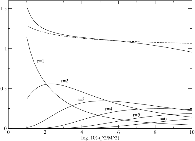
Figure 5: Contributions $M_{0;2}^{(r)}$ for $n=3$ from $r=1,\dots,6$–particle states. The upper full line is their sum. The dashed line is the perturbative expansion of $M_{0;2}+{\widetilde{M}}_{0;2}=1+\lambda$ up to and including terms of order $\lambda(q^{2})$.

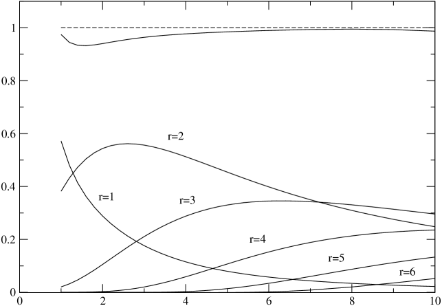
Figure 6: As for Fig. 5 but for the moment $l=1,N=1$; here the PT result is $1+{\rm O}(\lambda^{2})$.

4.3 Conclusions

Many qualitative field–theoretic features first observed in non–perturbative studies of integrable models in $2d$, have in the past found their counterparts in realistic models in 4 dimensions. Although fascinating in their own right, we hope that the investigations of structure functions of $2d$ O$(n)\,\,\sigma$–models presented in this paper will play a similar rôle. Similar methods are applicable to many other physical situations e.g. generalized structure functions, exclusive electro–production processes and rapidity gaps.

4.4 Acknowledgements

We would like to thank Ferenc Niedermayer for many instructive discussions on the parton model, Fred Jegerlehner for sending us data files on the QCD Adler function, Martin Lüscher and Christian Kiesling for reading the manuscript, and Vladimir Chekelian for information on the HERA data. This investigation was supported in part by the Hungarian National Science Fund OTKA (under T034299 and T043159).

References

- [1] A. Buras, Rev. Mod. Phys. 52 (1980) 199
- [2] G. Altarelli, Phys. Reports 81 (1982) 1
- [3] R. G. Roberts, The Structure of the Proton, Cambridge University Press, 1990
- [4] J. R. Forshaw, D. A. Ross, Quantum Chromodynamics and the Pomeron, Cambridge University Press, 1999
- [5] V. Gribov, L. Lipatov, Sov. J. Nucl. Phys. 15 (1972) 438 and 675; L. Lipatov, ibid 20 (1975) 94; Y. Dokshitser, Sov. Phys. JETP 46 (1977) 641
- [6] G. Altarelli, G. Parisi, Nucl. Phys. B126 (1977) 298
- [7] E. Kuraev, L. Lipatov, V. Fadin, Sov. Phys. JETP 44 (1976) 443; ibid 45 (1977) 199; Y. Balitskii, L. Lipatov, Sov. J. Nucl. Phys. 28 (1978) 822
- [8] E. Iancu, R. Venugopalan, hep-ph/0303204, to be published in QGP3, Eds. R. C. Hwa and X. N. Wang, World Scientific
- [9] L. McLerran, Acta Phys. Polon.B34 (2003) 5783; also hep-ph/0402137
- [10] Small Collaboration; B. Andersson et al., Eur. Phys. J. C25 (2002) 77; J. Andersen et al, hep-ph/0312333
- [11] A. H. Mueller, Summary talk given at 11th International Workshop on Deep Inelastic Scattering (DIS 2003), St.Petersburg, Russia, 23-27 Apr 2003, hep-ph/0307265
- [12] QCDSF-UKQCD Collaboration: T. Bakeyev et al. Contribution to 2nd Cairns Topical Workshop on Lattice Hadron Physics 2003 (LHP 2003), Cairns, Australia, 22-30 Jul 2003, hep-lat/0311017
- [13] J. W. Negele et al, hep-lat/0404005
- [14] A. M. Polyakov, Phys. Lett. 72B (1977) 224
- [15] M. Lüscher, Nucl. Phys. B135 (1978) 1
- [16] A. B. and Al. B. Zamolodchikov, Ann. Phys. 120 (1979) 253; Nucl. Phys. B133 (1978) 525
- [17] F. A. Smirnov, Form factors in Completely Integrable Models of Quantum Field Theory, World Scientific, 1992
- [18] M. Karowski, in Field theoretical methods in particle physics, 1980, ed. W. Rühl, Pg. 307
- [19] J. Balog, M. Niedermaier, F. Niedermayer, A. Patrascioiu, E. Seiler, P. Weisz, Phys. Rev. D60 (1999) 094508
- [20] J. Balog, M. Niedermaier, Phys. Rev. Lett. 78 (1997) 4151; Nucl. Phys. B500 (1997) 421
- [21] J. Balog, P. Weisz, in preparation
- [22] D. J. Gross, A. Neveu, Phys. Rev. D10 (1974) 3235
- [23] S. Eidelman, F. Jegerlehner, A. L. Kataev, O. Veretin, Phys. Lett. B454 (1999) 369
- [24] H1 Collab., C. Adloff et al., Eur. Phys. J. C21 (2001) 33
- [25] J. Balog, P. Weisz, Nucl. Phys. B668 (2003) 506
- [26] D. Buchholz, R. Verch, Rev. Math. Phys. 7 (1995) 1195; ibid 10 (1998) 775; D. Buchholz, Nucl. Phys. B469 (1996) 333; also, Talk at 12th International Congress of Math Phys (ICMP97), Brisbane, Australia 13-19 July 1997, hep-th/9710094
- [27] S. Caracciolo, A. Montanari, A. Pelissetto, JHEP 0009 (2000) 045; A. Montanari, Ph.D.Thesis, hep-lat/0104005
- [28] P. Hasenfratz, M. Maggiore, F. Niedermayer, Phys. Lett. B245 (1990) 522; P. Hasenfratz, F. Niedermayer, Phys. Lett. B245 (1990) 529