Symmetry allowed, but unobservable, phases in renormalizable Gauge Field Theory Models

Abstract:

In Quantum Field Theory models with spontaneously broken gauge invariance, renormalizability limits to four the degree of the Higgs potential, whose minima determine the vacuum state at tree-level. In many models, this bound has the intriguing consequence of preventing the observability, at tree-level, of some phases that would be allowed by symmetry. We show that, generally, the phenomenon persists also if one-loop radiative corrections are taken into account. The tree-level unobservability of some phases is characteristic in two-Higgs-doublet extensions of the Standard Model with additional discrete symmetries (to protect against neutral current flavor changing effects, for instance). We show that an extension of the scalar sector through suitable singlet fields can resolve the unnatural limitations on the observability of all the phases allowed by symmetry.

1 Introduction

In Quantum Field Theory models with spontaneously broken gauge invariance, at tree level, the true vacuum of the theory is determined by the location of the absolute minimum of the Higgs potential, thought of as a function of classical fields $\phi\in{\mathbb{R}}^{n}$. The set $\phi=(\phi_{1},\dots,\phi_{n})$ of all the scalar fields of the model transforms as an $n$-dimensional vector of the space of a linear representation of the full symmetry group (gauge group plus, possibly, discrete symmetries) of the Lagrangian (we shall denote by $G$ the linear group thus defined). The Higgs potential $V^{(d)}_{a}(\phi)$ is built as the most general G-invariant polynomial of given degree $d$ and is characterized also by a set $a=(a_{1},a_{2},\dots)$ of independent real coefficients determined by external conditions (control parameters). Generally the degree of the Higgs potential is chosen to be four, to guarantee renormalizability of the theory, and the control parameters are completely free, but for the constraints on the coefficients of the terms of highest degree in $\phi$, required to guarantee that $V^{(d)}_{a}(\phi)$ is bounded from below.

Owing to $G$-invariance, the absolute minimum of $V^{(d)}_{a}(\phi)$ is degenerate along a $G$-orbit $\Omega_{0}$, whose points define equivalent vacua. The set of subgroups of $G$ that leave invariant (isotropy subgroups of $G$ at) the points of $\Omega_{0}$ form a conjugacy class $[G_{0}]=\{g\,G_{0}\,g^{-1}\mid g\in G\}$, that defines both the orbit type of $\Omega_{0}$ and the residual symmetry of the system after spontaneous symmetry breaking. We shall think of this symmetry as thoroughly characterizing the phase of the system.

Distinct $G$-orbits can have the same symmetry and orbits with the same symmetry are said to form a stratum. Minima of the Higgs potential located at orbits lying in the same stratum determine the same phase: there is a one-to-one correspondence between strata and phases allowed by the $G$-symmetry.

An allowed phase can be dynamically realized as a phase of the system at tree-level only if the Higgs potential develops an absolute minimum at an orbit of the corresponding stratum, for at least a choice of values in the range of the control parameters. This possibility is strongly conditioned by the degree of the polynomial $V^{(d)}_{a}(\phi)$, which has to be chosen $\leq 4$, if one likes to guarantee the renormalizability of the model.

Generally, by varying the values of the control parameters, the location of the absolute minimum of the Higgs potential can be moved to different strata. When this happens, structural phase transitions take place [1]:

1. The transition is said second order if a continuous variation of the control parameters determines a continuous displacement of the location of the absolute minimum to a contiguous stratum and a consequent abrupt change of the residual symmetry. The initial and final symmetries are necessarily linked by a group-subgroup relation.

2. The transition is said first order if, for some values of the control parameters, the absolute minimum of the potential coexists with a faraway local minimum, sitting in a different (not necessarily contiguous) symmetry stratum. As the control parameters vary, the local minimum becomes deeper than the original global minimum, which is first transformed into a metastable local minimum and, subsequently, may even disappear. The details of the phase transformation process may be different, depending on the physical problem one is dealing with. According to the delay convention the system state remains in a stable or metastable equilibrium state until such state disappears. According to the Maxwell convention, the system state always corresponds to the global minimum of the potential. These two conventions represent extremes in a continuum of possibilities (see [2]). Quite recently, the impact of a delay-like convention (i.e. the requirement that the electroweak vacuum is sufficiently long-lived) on the lower bounds on the Higgs mass has been analyzed [3].

A phase will be said to be stable if it is associated to a non-degenerate absolute minimum of $V^{(d)}_{a}(\phi)$ which is stable in its stratum, stability being intended in the sense that small arbitrary perturbations of the control parameters in their allowed range cannot push the location of the minimum in a different stratum. Generally, only stable phases are thought to have non-zero probability to be observed. Therefore, in this paper, we shall identify the observable phases of a model with the allowed phases which can be stable in the dynamics of the model.

Our attitude in the analysis of the critical points of an Higgs potential is suggested by Catastrophe Theory, whose aim is to classify the modifications in the qualitative nature of the solutions of equations depending on (control) parameters, as these are varied. A particularly interesting class of equations is formed by gradient systems, i.e. autonomous dynamical systems, in which the (generalized) forces can be derived from the gradient of some potential. In particular, Elementary Catastrophe Theory studies the way the equilibria of a potential are modified as the control parameters are varied [4]. In this framework, a potential is considered as structurally stable if its qualitative properties (number and types of critical points, basin of attractions, etc.) are not changed by a sufficiently small perturbation of the control parameters. In a $n$-parameter family of functions, Morse functions are generic, i.e. are structurally stable. Thus, in a model describing the evolution of our Universe through a phenomenological potential, consisting in a $n$-parameter family of functions, it is natural to assume that a physically realizable phase corresponds to a generic configuration. Non-Morse potential functions have the role of organizing the entire qualitative nature of the family of functions, determining the possible phase transitions.

A model in which all the allowed phases are observable will be said to be complete.

It is not difficult to guess that, if in a model the degree of the Higgs potential is allowed to be sufficiently high, then the model is complete [5]. On the contrary, if the degree of the potential is limited, for instance to guarantee the renormalizability of the model, some allowed phases may become unobservable at tree-level. This fact has been more or less known since a long time, but has never attracted the due attention, mainly because, after the paper by S. Coleman and E. Weinberg (hereafter referred to as CW [6]) it is widely belived that the problem can always be removed by radiative corrections, whose contributions to the “effective” Higgs potential consist in $G$-invariant polynomials in $\phi$, of increasing degrees at increasing perturbative orders.

One of the main goals of this paper is to prove that this widespread belief is based on an unjustified extensive interpretation of the CW results, in the sense that the inclusion of radiative corrections is not in general, sufficient to cure the tree-level incompleteness of a gauge model. This statement will be proved to be true in a (SO${}_{3}\times{\mathbb{Z}}_{2}$, 5) model studied by CW, in an (SO₃, 5) variant of the model and in an (SU₃, 8) model.

The reason why radiative corrections may result ineffective in removing a tree-level incompleteness of a model, is due to the fact that, in the $G$-invariant polynomials in $\phi$, yielding the contributions of radiative corrections, the coefficients are well determined functions of the parameters defining the Lagrangian of the model at tree-level, and cannot, therefore, play the role of arbitrary independent parameters, like the control parameters.

It is also worth recalling that, in spontaneously broken gauge symmetries, the exact effective potential is real, while its perturbative series can be complex (see for instance [7, 8, 9, 10]). So, besides the computational difficulties in the determination of the quantum contributions to the (perturbative) effective potential, which essentially limit the results to one- or two-loop effects, particular care has to be taken in the regions where the effective quantum potential is complex.

We consider quite intriguing the emergence, in the set of allowed phases of a model, of possible selection rules originating from the constraint posed by the request of renormalizability. Our point of view is that renormalizability, which actually has to be considered as a “technical” assumption required to allow a consistent and significant perturbative solution of the theory, should not limit the implications of the basic symmetry of the formalism used to describe the system [11], not even at tree-level. In other words, in our opinion, all the allowed phases should be observable already at tree-level in a viable model. This attitude, if accepted, may have important consequences in the study of of Electro-Weak (EW) phase transitions, in the sense that all the allowed phases have to be thought, in principle, as possible phases in the evolution of the Universe [12, 13].

In the Standard Model (SM) of EW interactions, although the gauge boson and fermion structure has been accurately tested, experimental information about the Higgs sector (HS) is still very weak (see, for instance, [14, 15] and references therein). Serious motivations are well known for the extension of the scalar sector; among them we just recall supersymmetry (SUSY) and baryogenesis at the EW scale, [16]. So far, various extensions of the SM have been devised: the Minimal SUSY SM, the SM plus an extra Higgs doublet, the MSSM plus a Higgs singlet, the left–right symmetric model, the SM plus a complex singlet Higgs (see the introduction to [17] and references therein); quite recently, even a partly supersymmetric SM has been conceived ([18]). There is still, therefore, a certain freedom in the choice of the Higgs sector of the theory. A second goal of this paper is to show how compatibility between tree-level completeness and renormalizability can give further inputs in its construction.

In particular we shall show that, while in the basic two-Higgs-doublet extension of the SM all the allowed phases are observable, in the most popular models with two Higgs doublets, if the usual additional discrete symmetries are added to avoid flavor changing neutral current (FCNC) effects, this is only true if the Higgs potential is a polynomial of sufficiently high degree, greater than four.

Nowadays, there is general agreement in considering the Standard Model (SM) as an effective theory [19, 20, 21], since, for example, higher order (non renormalizable) operators are generally required to describe non vanishing neutrino masses. So, the main attitudes in dealing with phenomenology are either thinking to the SM as a low energy limit of a (supersymmetric) Grand Unification Theory (GUT) or to disregard the parent high energy theory and trying to recover, in a model independent way, some knowledge on bounds to the GUT unification scale, used to suppress higher order operator contributions to low energy physics. String theory is a major (but not the only!) candidate for this high energy theory, having the capability to include gravitation in a unique framework.

Despite this and even if it is only a technical requirement, one may wonder whether renormalizability can be maintained, without limiting the symmetry content of the theory. We shall show that, in some tree-level incomplete two-Higgs-doublet models, symmetry and renormalization can be reconciled if the Higgs sector is extended with the addition of one or more scalar singlets, with convenient transformation properties under the discrete symmetries of the model.

The paper is organized in the following way. In Section 2, making systematic use of simple results and techniques of geometric invariant theory [24], which strongly simplify the calculations, we determine all the allowed phases of three simple models: an (SO${}_{3}\times{\mathbb{Z}}_{2},{\underline{5}}$)–model studied as an example by CW, a simple (SO${}_{3},{\underline{5}})$ variant of the same model and, finally, an (SU₃, ${\underline{8}}$)–model. We show that all these models are tree-level incomplete and that the incompleteness is not removed if one-loop radiative corrections are taken into account. In Section 3 we justify the formal approach followed in Section 2, recalling the basic elements of a general approach (orbit space approach) to the determination of all the allowed phases [22, 23, 5] of a gauge model. Section 4 is devoted to the determination of allowed and observable phases in two Higgs doublet (2HD) extensions of the Standard Model in different dynamical configurations (renormalizable and incomplete or non-renormalizable and complete). In particular, besides the basic 2HD model with gauge and symmetry group SU${}_{2}\times\mathrm{U}_{1}$, we shall examine a 2HD model with an additional FCNC protecting discrete symmetry and a model in which the symmetry group is further extended with the inclusion of a CP-like transformation. In Section 5, we show that the extensions of these models with the introduction of convenient additional scalar singlets allows to make them complete, without giving up renormalizability.

2 Allowed and observable phases in three simple gauge models

In this section we shall determine all the allowed phases of three simple models: an (SO${}_{3}\times{\mathbb{Z}}_{2},{\underline{5}}$)–model studied as an example by CW, a simple (SO${}_{3},{\underline{5}})$ variant of the same model and an (SU₃, ${\underline{8}}$)–model. We show that:

1. the renormalizable versions of all these models are tree-level incomplete;

2. the incompleteness persists if the tree-level Higgs potential is replaced with the one-loop effective potential;

3. the incompleteness is completely removed at tree-level if one gives up renormalizability and allows a sufficiently high degree polynomial Higgs potential.

We shall be highly facilitated in our calculations by a systematic use of simple techniques and results of geometric invariant theory, that will be illustrated in a general formulation, in the next section.

2.1 An (SO₃, 5) gauge model

The model is a slight modification of an (SO${}_{3}\times{\mathbb{Z}}_{2},{\underline{5}})$ model, studied by CW, that will be analyzed in the following subsection.

The gauge (and complete symmetry) group of the model is SO₃ and the Higgs fields transform as the components of a vector $\phi$ in the space of a real five dimensional orthogonal representation of the group. If the components of $\phi$ are ordered in a $3\times 3$ traceless symmetric matrix $\Phi(\phi)$:

$$\Phi(\phi)=\frac{1}{\sqrt{2}}\,\left(\begin{array}[]{ccc}\phi_{4}+\phi_{5}/\sqrt{3}&\phi_{1}&\phi_{2}\\ \phi_{1}&-\phi_{4}+\phi_{5}/\sqrt{3}&\phi_{3}\\ \phi_{2},&\phi_{3}&-2\phi_{5}/\sqrt{3}\end{array}\right),$$ (1)

their transformation properties under a transformation $\gamma\in\mathrm{SO}_{3}$ are specified by the following relations:

$$\Phi(\phi)\rightarrow\Phi(\phi^{\prime})=\gamma\,\Phi(\phi)\,\gamma^{-1},\hskip 25.0pt\phi^{\prime}_{i}=\sum_{j=1}^{5}\,g_{ij}\,\phi_{j},$$ (2)

which determine the matrices $g$ forming the linear group $G$. This group has only two basic homogeneous invariant polynomials, that can be conveniently chosen to be the following:

$$p_{1}(\phi)={\rm Tr}\,\Phi^{2}(\phi),\hskip 25.0ptp_{2}(\phi)=\sqrt{6}\,{\rm Tr}\,\Phi^{3}(\phi).$$ (3)

In particular $p_{1}(\phi)=\sum_{i=1}^{5}\,\phi_{i}^{2}$, assuring that, as claimed, the group $G$ is a group of orthogonal matrices.

A general fourth degree $G$-invariant polynomial, to be identified with the Higgs potential of a renormalizable version of the model, can be conveniently written in the following form, in terms of the basic polynomial invariants $p=(p_{1},p_{2})$:

$$V^{(4)}_{a}(\phi)=\widehat{V}^{(4)}_{a}(p(\phi)),$$ (4)

where

$$\widehat{V}^{(4)}_{a}(p)=a_{1}\,p_{1}+a_{2}\,p_{2}+a_{3}\,p_{1}^{2},\hskip 25.0pta=(a_{1},a_{2},a_{3})$$ (5)

and $a_{3}$ has to be positive to guarantee that the potential is bounded from below for arbitrary $a_{1}$ and $a_{2}$.

A determination of the stationary points of $V^{(4)}_{a}(\phi)$ with standard analytic methods is not easy, even in this simple case, so it is convenient to tackle the problem in a cleverer way. Since, as stressed in the Introduction, one is essentially interested only in the location of the $G$-orbit at which $V^{(4)}_{a}(\phi)$ takes on its minimum, and a $G$-invariant function is a constant along a $G$-orbit, it will be advantageous to express $V^{(4)}_{a}$ as a function of the $G$-orbits. The approach followed by CW points in this direction. In fact, they exploit the fact that the matrix $\Phi(\phi)$ can be diagonalized by an SO₃ transformation (see (2)). This means that in every $G$-orbit there is at least a point $\phi$ represented by a diagonal matrix $\Phi(\phi)$, so the minimization problem can be tackled with the additional conditions $\phi_{1}=\phi_{2}=\phi_{3}=0$, an expedient that make it easily solvable. Even if effective in simple cases, like the one we are considering, this approach has two shortcomings:

1. The diagonalization of $\Phi(\phi)$ does not lead to a unique result. From a geometrical point of view, the different results correspond to the distinct intersections of the $G$-orbit through $\phi$ with a convenient orthogonal hyperplane and, in the case of compact groups, these intersections are always multiple. In the present case, for fixed $(x,y)\in{\mathbb{R}}^{2}$ and $\phi_{1}=\phi_{2}=\phi_{3}=0$, the six distinct points $(\phi_{4},\phi_{5})=(\pm x,y),\ (\pm(x-\sqrt{3}y)/2,\ -(\sqrt{3}x+y)/2),\ ((\pm x+\sqrt{3}y)/2,(-\sqrt{3}x+y)/2)$ lie on the same orbit. Thus, the coordinates $(\phi_{4},\phi_{5})$ do not yield a one-to-one parametrization of the orbits of $G$.

2. The approach cannot be generalized to an arbitrary compact linear group $G$.

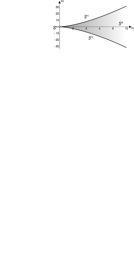
Figure 1: Orbit space and symmetry strata of (SO${}_{3},\underline{5})$ gauge model.

Both these difficulties can be overcome using a fundamental property of the basic invariants of any compact linear group: at distinct orbits, $p$ takes on distinct values (see next section).

Therefore, $(p_{1},p_{2})$ can be used as coordinates of the orbits of $G$ and the minimization of $V^{(4)}_{a}(\phi)=\widehat{V}^{(4)}_{a}(p(\phi))$ can be reduced to the minimization of $\widehat{V}^{(4)}_{a}$, thought of as a function of the independent variables $(p_{1},p_{2})$.

This choice yields, as additional significant bonus, a sensible reduction of the degree of the polynomial to minimize: $\widehat{V}^{(4)}_{a}(p)$ is only second degree in $p_{1}$ and linear in $p_{2}$. The sole price to pay for these advantages is that the range of $p$ does not coincide with the real $p$-plane and the minimization problem for $\widehat{V}^{(4)}_{a}(p)$ has to be dealt with as a constrained minimization problem. But this is a solvable problem. The range of $p$ can, in fact, be easily determined in the following way. The rectangular matrix formed by the gradients of the basic invariants, multiplied by its transpose, defines a positive semi-definite matrix

$${P_{\alpha\beta}(\phi)=\sum_{i=1}^{5}\,\frac{\partial p_{\alpha}(\phi)}{\partial\phi_{i}}\,\frac{\partial p_{\beta}(\phi)}{\partial\phi_{i}},\hskip 25.0pt\phi\in{\mathbb{R}}^{5},\ \alpha,\beta=1,2,}$$ (6)

whose elements are $G$-invariant polynomials in $\phi$, since the group $G$ is a group of orthogonal matrices.

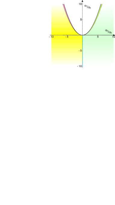
Figure 2: Representation of the solution of the minimization problem for the (SO${}_{3},{\underline{5}}$ )–model in the space of the control parameters.

In fact, taking into account also the homogeneity properties of $p_{1}$ and $p_{2}$, one easily finds

$${P(\phi)=\widehat{P}(p(\phi)),\quad\widehat{P}(p)=\left(\begin{array}[]{rr}4\,p_{1}&6\,p_{2}\\ 6\,p_{2}&9\,p_{1}^{2}\end{array}\right).}$$ (7)

The following conditions, assuring the semi-positivity of the matrix $\widehat{P}(p)$, define the range $p({\mathbb{R}}^{5})$ in the $p$-space (see Fig. 1):

$$p_{1}^{3}-p_{2}^{2}\geq 0.$$ (8)

As stated in the Introduction, the points $p$ in the range $p({\mathbb{R}}^{5})$ of $p(\phi)$ are in a one-to-one correspondence with the $G$-orbits. Thus, the algebraic set $p({\mathbb{R}}^{5})$ can be identified with the orbit space ${\mathbb{R}}^{5}/G$ of $G$.

The validity and meaning of condition (8), and, particularly, of the limiting cases, can be easily understood if it is written in terms of $\phi$, for $\phi_{1}=\phi_{2}=\phi_{3}=0$:

$$p_{1}^{3}(\phi)-p_{2}^{2}(\phi)\mid_{\phi_{1}=\phi_{2}=\phi_{3}=0}=\phi_{4}^{2}\left(\phi_{4}^{2}-3\phi_{5}^{2}\right)^{2}\geq 0.$$ (9)

A remarkable fact, which is characteristic of the orbit spaces of all compact groups, is the following. Being the orbit space a connected semi-algebraic set, it presents a natural geometric stratification (disjoint partition) in connected manifolds (primary strata), each primary stratum being open in its topological closure and contained, but for the highest dimensional one which is unique (principal stratum), in the boundary of a higher dimensional primary stratum. In the present case the primary strata (shown in Fig. 1) correspond to the following algebraic manifolds $W^{(i)}_{j}$ (the apex $i$ indicates the dimension and $j$ is an order index):

$${\begin{array}[]{lcl}W^{(0)}:\ p_{1}=0=p_{2};&&W^{(1)}_{1}:\ p_{1}>0=p_{2}-p_{1}^{3/2};\\ W^{(1)}_{2}:\ p_{1}>0=p_{2}+p_{1}^{3/2};&&W^{(2)}:\ p_{2}^{2}<p_{1}^{3}.\end{array}}$$ (10)

The symmetry strata are formed by one or more primary strata with the same dimensions. This property reduces the determination of all the symmetry strata, i.e. of all the allowed phases, to the determination of the solutions of the equation

$${g\,\Phi(\phi)\,g^{-1}=\Phi(\phi),\hskip 25.0ptg\in\mathrm{SO}_{3},}$$ (11)

only for a few configurations of $\Phi(\phi)$, one for each primary stratum, and, for each primary stratum, $\Phi(\phi)$ can be chosen in such a way that the solution turns out to be particularly simple.

Good choices of $\phi$ for an easy determination of the solutions of (11) are, for instance, $\phi=(0,0,0,0,-1)$, $\phi=(0,0,0,0,+1)$ and $\phi=(0,0,0,1,0)$ for $W^{(1)}_{1}$, $W^{(1)}_{2}$ and $W^{(2)}$, respectively. Using also (2) one easily concludes that

• The $G$-orbit corresponding to the point $\phi=0$ is represented by the tip of the orbit space and forms a stratum $S^{(0)}$, formed by a unique orbit with symmetry $[SO_{3}]$, corresponding to the phase ${\mathcal{F}}^{(0)}$ with unbroken symmetry.

• The other SO₃-orbits lying on the boundary of the orbit space, characterized by the conditions $p_{1}^{3}=p_{2}^{2}>0$ $(\phi_{1}=\phi_{2}=\phi_{3}=\phi_{4}^{2}\left(\phi_{4}^{2}-3\phi_{5}^{2}\right)^{2}=0\neq\phi_{4}^{2}+\phi_{5}^{2}$), share the same symmetry [SO₂]. They form, therefore, a unique stratum $S^{(1)}$, corresponding to a phase ${\mathcal{F}}^{(1)}$: $S^{(1)}=W^{(1)}_{1}\cup W^{(1)}_{2}$.

• Generic SO₃-orbits, corresponding to interior points of the orbit space, characterized by $p_{1}^{3}>p_{2}^{2}$ ($\phi_{1}=\phi_{2}=\phi_{3}=0<\phi_{4}^{2}\left(\phi_{4}^{2}-3\phi_{5}^{2}\right)^{2}$) have trivial symmetry (isotropy subgroup $\{1\!\!1\}$). They form, therefore a unique stratum $S^{(2)}$, corresponding to a phase ${\mathcal{F}}^{(2)}$ with completely broken symmetry: $S^{(2)}=W^{(2)}$.

Let us now examine the tree-level observability of the three allowed phases just found, in the assumption that the dynamics in the Higgs sector is determined by the potential (5). For this purpose, we have only to check whether, for each stratum $S^{(i)}$, there is an exclusive three dimensional region $R^{(i)}$ in the space of the control parameters $a=(a_{1},a_{2},a_{3})$, such that, for $a\in R^{(i)}$ the function $\widehat{V}^{(4)}_{a}(p),\ p\in{\mathbb{R}}^{n}/G$ has a stable absolute minimum located in $S^{(i)}$.

For general values of $a_{2}$, $\widehat{V}^{(4)}_{a}(p)$ is linear in $p_{2}$. So, one immediately realizes that, for any fixed value of $p_{1}$, it takes on its absolute minimum when $p_{2}$ is maximum (for $a_{2}<0$) or minimum (for $a_{2}>0$), that is on the boundary of the orbit space, formed by the union of the strata $S^{(0)}$ and $S^{(1)}$. Only for $a_{2}=0$ and $a_{1}<0$ the absolute minimum is located in the principal stratum $S^{(2)}$, but it is degenerate along a line $p_{1}=-a_{1}/(2a_{3})$, which also crosses the stratum $S^{(1)}$. Any perturbation $\delta a_{2}\neq 0$ would move it to $S^{(1)}$, so it is unstable.

A complete analytic solution of the minimization problem leads to the following results (see Fig. 2):

1. For $a_{1}<a_{2}^{2}/(4a_{3})\neq 0$ (open region below the lower parabola in Fig. 2), the absolute minimum is stable in the stratum $S^{(1)}$.

2. For $a_{1}>a_{2}^{2}/(4a_{3})$ the absolute minimum is stable in the stratum $S^{(0)}$.

3. For $9a_{2}^{2}/(32a_{3})>a_{1}>a_{2}^{2}/(4a_{3})$ (open region between the two parabolas in Fig. 2) the absolute minimum in $S^{(0)}$ is stable and coexists with a higher stable local minimum in $S^{(1)}$.

4. For $a_{1}<0=a_{2}$, the absolute minimum is degenerate and, therefore,  unstable, across the strata $S^{(1)}$ and $S^{(2)}$.

5. The parabola of equation $a_{1}=a_{2}^{2}/(4a_{3})$ is a critical line, formed by first order phase transition points.

If the evolution of the Universe were described by this model, it would be represented by a continuous line in the space of the control parameters $(a_{1},a_{2},a_{3})$. The only observable phase transitions would be first order transitions between the phases ${\mathcal{F}}^{(0)}$ and ${\mathcal{F}}^{(1)}$. These results can be easily understood graphically, noting that the level curves (equipotential lines) in the $p$-plane are parabolas (see Fig. 3). Therefore, the critical lines in the plane $(a_{1}/a_{3},a_{2}/a_{3})$ can be easily determined (see Fig. 2).

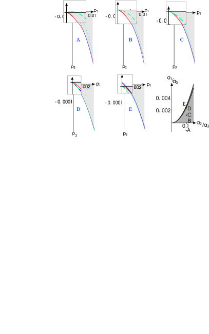
Figure 3: Level curves corresponding to critical points located in the primary strata $W^{(1)}_{2}$ (blue, continuous line) and $W^{(0)}$ (dashed green line) for the (SO${}_{3},{\underline{5}})$ gauge model (renormalizable version). The border of the orbit space in drawn in red. Cases A … E refer to the values of the control parameter shown in the last figure (for $a_{3}=1$ and $a_{2}/a_{3}=0.1$). The region near the origin of the plane $(p_{1},p_{2})$ is magnified, to show that the level curve for $W^{(0)}$ is tangent to the $p_{1}$ axis, in figure B. In figure D a typical coexistence of two degenerate minima is shown.

2.1.1 A non-renormalizable version of the model

Let us now show that if the Higgs potential is chosen as a general $G$-invariant polynomial of degree six, so that it contains also a term proportional to $p_{2}^{2}(\phi)$, then all the allowed phases turn out to be observable at tree-level. Like in the previous subsection, let us define $V^{(6)}_{a}(\phi)=\widehat{V}^{(6)}_{a}(p(\phi))$, through the relation

$$\widehat{V}^{(6)}_{a}(p)=a_{1}\,p_{1}+a_{2}\,p_{2}+a_{3}p_{1}^{2}+a_{4}\,p_{1}\,p_{2}+a_{5}\,p_{1}^{3}+a_{6}\,p_{2}^{2}.$$ (12)

For arbitrary values of $a=(a_{1},\dots,a_{6})$, the restriction of the function $\widehat{V}^{(6)}_{a}(p)$ to the orbit space is bounded from below if $a_{5}>0$ and $a_{6}>-a_{5}$.

The fact that all the allowed phases are observable can be proved through explicit standard calculations, but we prefer a more intuitive approach, that can be generalized to the case of an arbitrary linear compact group $G$, with a free basis of basic polynomial invariants.

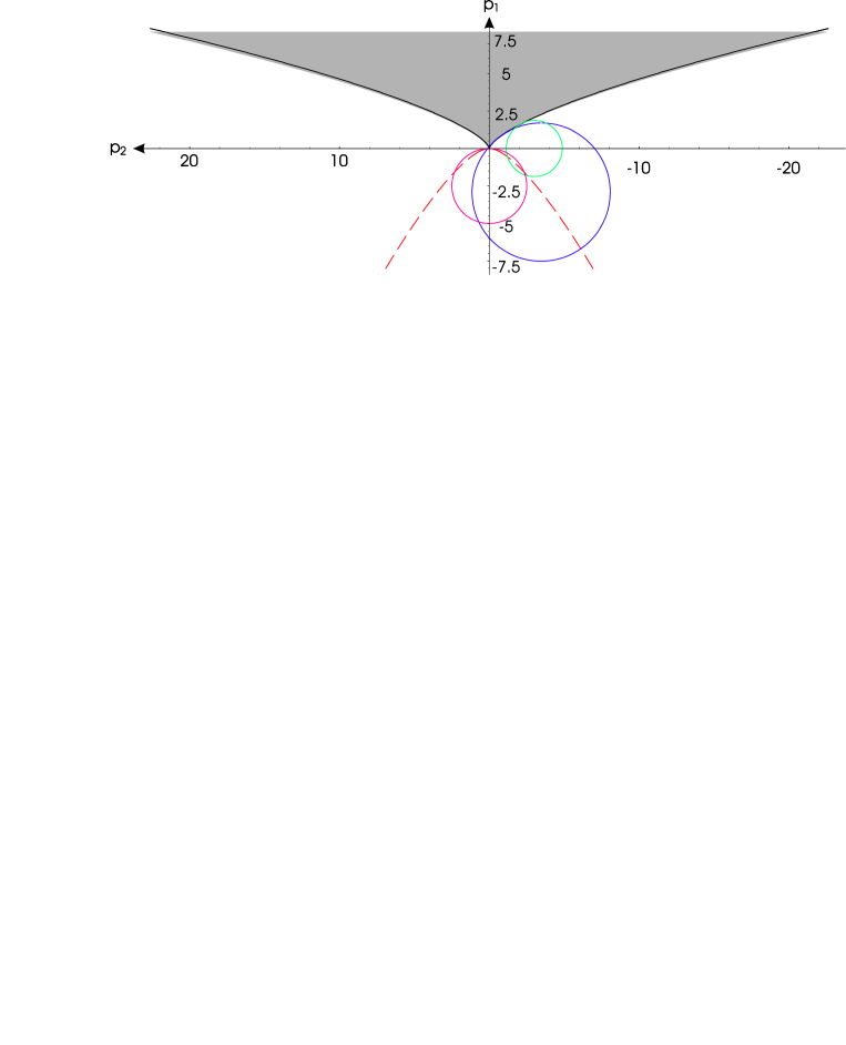
Figure 4: Level curves corresponding to critical points located in the primary strata $W^{(1)}_{2}$ (green circle) and $W^{(0)}$ (magenta circle) for the complete non renormalizable version of the (SO${}_{3},{\underline{5}})$ gauge model, for $a=a^{(0)}=(a_{1},a_{2},1,0,0,1)$. The dashed red curve represents the Maxwell catastrophe projection, which is the evolute of the curve $S^{(1)}$, that is the locus of the points in which degenerate absolute minima coexist in $S^{(1)}$ and $S^{0}$. The values of the control parameter can be recovered through the identification $a_{1}=-2\eta_{1}$ and $a_{2}=-2\eta_{2}$. The equation of the critical curve is $6561{p_{2}}^{4}+288(1+54p_{1})\,{p_{2}}^{2}+512p_{1}(1+6p_{1})^{2}=0$. The region external to the orbit space can be divided into three connected parts: when $\eta$ is in the first region, extending towards $p_{1}\rightarrow-\infty$ the minimum is in $S^{(0)}$, while in the other two regions, the minimum lies in the singular stratum $S^{(1)}$ (on $W^{(1)}_{1}$ and $W^{(1)}_{2}$, respectively, for $\eta_{1}>0$ and $\eta_{1}<0$.)

Let us denote by $a^{(0)}$ the following particular choice of values for the control parameters $a=(a_{1},\dots,a_{6})$:

$${a^{(0)}=(a_{1},a_{2},1,0,0,1),}$$ (13)

where the coefficients $a_{1}$ and $a_{2}$ of the linear terms in $\widehat{V}^{(6)}_{a}(p)$, are still considered as arbitrary parameters. Then, $\widehat{V}^{(6)}_{a^{(0)}}(p)$ can be rewritten in the following suggestive form:

$${\widehat{V}^{(6)}_{a^{(0)}}(p)=\left(p_{1}-\eta_{1}\right)^{2}+\left(p_{2}-\eta_{2}\right)^{2}+C,\hskip 25.0ptp\in p({\mathbb{R}}^{5}),}$$ (14)

where,

$${\eta_{1}=-a_{1}/2,\hskip 25.0pt\eta_{2}=-a_{2}/2,\hskip 25.0ptC=-{\eta_{1}}^{2}-{\eta_{2}}^{2}.}$$ (15)

In the $p$-space ${\mathbb{R}}^{2}$, the polynomial $\widehat{V}^{(6)}_{a^{(0)}}(p)-C$ represents the squared distance between the point $\eta$ and the point $p$ of the orbit space. It is therefore clear that

1. For $\eta$ interior to the orbit space, $V^{(6)}_{a^{(0)}}(p)$ has a stable (against small perturbations of its coefficients $\eta_{1}$ and $\eta_{2}$) absolute minimum at $p=\eta\in S^{(2)}$.

2. For $\eta$ exterior to the orbit space, but not too far from, and $\eta_{1}>0$, $\widehat{V}^{(6)}_{a^{(0)}}(p)$ has a stable absolute minimum at the closest point of $S^{(1)}$ to $\eta$.

3. For $\eta$ exterior to the orbit space and $\eta_{1}<0$, $\widehat{V}^{(6)}_{a^{(0)}}(p)$ has a stable absolute minimum in $S^{(0)}$.

4. For $\eta_{1}=0$, $\widehat{V}^{(6)}_{a^{(0)}}(p)$ has an unstable absolute minimum at $p=0$.

5. For $\eta\in S^{(1)}$, $\widehat{V}^{(6)}_{a^{(0)}}(p)$ has an unstable absolute minimum at $p=\eta$.

Let us now show that, the conclusions listed in the first three items above, about the existence of stable absolute minima in all the strata, continue to hold for $\widehat{V}^{(6)}_{a}(p)$, if $a$ ranges in a convenient domain, close to $a^{(0)}$.

To this end, in the range of the vector control parameters $a$ ($a_{5}>0$), for each arbitrarily chosen couple of non critical values of $(a_{1},a_{2})$ ($a_{1}\,a_{2}\neq 0$), let us consider points $a$ which are sufficiently close to $a^{(0)}$. Continuity reasons assure that, for every choice of $a$ in this region, the polynomial $\widehat{V}^{(6)}_{a}(p)$ has a stable local minimum close to the location $p^{(0)}$ of the minimum of $\widehat{V}^{(6)}_{a^{(0)}}(p)$ and sitting on the same stratum. In fact, the existence of a stationary point of $\widehat{V}^{(6)}_{a}(p)$ close to $p^{(0)}$ is guaranteed by the inverse functions theorem and this stationary point is surely an absolute minimum, since $\widehat{V}^{(6)}_{a}(p),\ p\in p({\mathbb{R}}^{5})$ is a convex function.

Let us denote by $v_{a}$ the minimum value of $\widehat{V}^{(6)}_{a}(p),\ p\in p({\mathbb{R}}^{5})$. Then the analytic justification just given is easy to understand from an analysis of the family of equipotential lines $\widehat{V}^{(6)}_{a}(p)=v_{a}$, for $a$ near to $a^{(0)}$ (see Fig. 4).

Figure 5: Level curve deformation for the non-renormalizable version of the (SO${}_{3},{\underline{5}}$) gauge model. The following values for the control parameters have been chosen: $a_{1}\approx-4.3$, $a_{2}\approx 6.18918$, $a_{3}=a_{4}=0.1$, $a_{6}\approx 0.998196$, in such a way that the centre of the ellipsis corresponding to $a_{5}=0$ is in point $(-2,-3)$ in the orbit space plane $(p_{1},p_{2})$. For this configuration the ellipsis turns out to be tangent to the orbit space primary stratum $W^{(1)}_{2}$ in the point of abscissa $p_{1}\approx 1.07322$. The sequence of plots shows how the aspect of the level curve changes according to different values of $a_{5}$ parameter.

1. For $a=a^{(0)}$ these lines are obviously circles centered at $\eta$. They are tangent to the orbit space for $\eta$ exterior to the orbit space (at a point of $S^{(1)}$, for $\eta_{1}>0$ and at $S^{(0)}$ for $\eta_{1}<0$), while they reduce to the point $\eta$, for $\eta$ interior to the orbit space.

2. When $a_{3}$, $a_{4}$ and $a_{6}$ are slightly perturbed, the circle is slightly deformed to an ellipsis centered in a point near to $\eta$, but, for the rest, the situation does not essentially change.

3. When also $a_{5}$ is raised to a small positive value, the geometry of the equipotential lines abruptly changes, but the conclusions remain essentially the same indicated above: the ellipsis is further slightly deformed, but remains a closed curve around $\eta$, and a new open branch of the algebraic curve is generated. The new branch, however, is confined to the far negative $p_{1}$-half-plane, if $a_{5}$ is sufficiently small. So it does not intersect the orbit space and cannot, consequently, host a minimum of the Higgs potential.

Before analyzing, in the next subsection, the effects of the contributions of one-loop radiative corrections to the effective potential, let us remark the following interesting aspect of the orbit space approach to the minimization problem we have followed. It has been proved in [25] that all the linear compact groups, whose base of invariant polynomials reduces to two elements with the same degrees $(d_{1},d_{2})$, have isomorphic orbit spaces. This means that the basic polynomial invariants can be chosen so that the $\widehat{P}$-matrix has a universal form, which, for $(d_{1},d_{2})=(2,3)$ is specified in (7). Since the general form of a given degree Higgs potential only depends on the number and degrees of the basic polynomial invariants, for all the groups under consideration, the minimization problem of the Higgs potential at tree-level reduces to the same geometrical problem. Only the symmetry of the possible phases depend on the particular symmetry group. The third sample model studied below, will yield an example of this phenomenon.

2.1.2 One-loop radiative corrections

In this subsection, we shall prove that the one-loop radiative corrections are not sufficient to make observable the phase ${\mathcal{F}}^{(2)}$, which is tree-level unobservable.

As stressed in CW, the vector bosons are responsible for the dominant radiative contributions $V_{\rm g}$ to the one-loop effective potential. In order to calculate $V_{\rm g}$, which is an SO₃-invariant function, in terms of the “coordinates” $p$, let us denote by $\langle\cdot,\cdot\rangle$ the euclidian scalar product in ${\mathbb{R}}^{5}$, by $T^{a}$, $a=1,2,3$ the generators of the Lie algebra of the matrix group $G$ and by $\epsilon^{a}$ the usual generators of the Lie algebra of the group SO₃:

$${\epsilon^{a}_{ij}=-\epsilon_{aij},\hskip 25.0pta,i,j=1,2,3.}$$ (16)

Then,

$${T^{a}\cdot\Phi=\epsilon^{a}\,\Phi-\Phi\,\epsilon^{a}.}$$ (17)

The explicit form of $V_{\rm g}(\phi)$ is the following [6]:

$${V_{\rm g}(\phi)=\frac{3}{64\pi^{2}}\,{\rm Tr}\left[M^{4}(\phi)\,\ln M^{2}(\phi)\right],}$$ (18)

where the matrix elements of $M^{2}(\phi)$ are defined by

$${M_{ab}^{2}(\phi)=g^{2}\,\langle T_{a}\phi,T_{b}\phi\rangle.}$$ (19)

The eigenvalues of the matrix $M^{2}(\phi)$ are SO₃-invariant algebraic functions of $\phi$ and the sum of all the products of $k$ distinct eigenvalues can be easily calculated as the sum $\sigma_{k}$ of the principal minors of order $k$, $k=1,2,3$. They are $G$-invariant polynomials in $\phi$ and can, therefore, be written as polynomial functions of $p$. A direct calculation gives

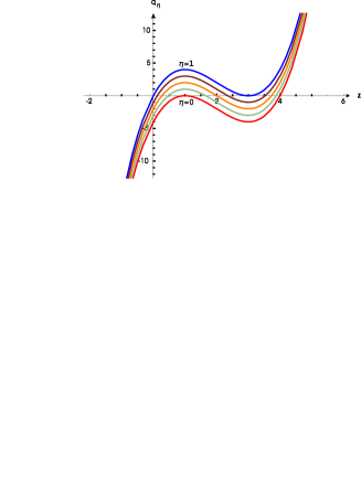
Figure 6: Family of functions $q_{\eta}(z)$, in the interval $[0,1]$ for $\eta=0,\;1/4,\;1/2,\;3/4,\;1$.

Figure 7: Graph of the function $f(\eta)=\sum_{i=1}^{3}z_{i}^{2}(\eta)\mathrm{ln}\left(z_{i}(\eta)\right)$

$${\begin{array}[]{l}\sigma_{1}=6\,p_{1},\hskip 25.0pt\sigma_{2}=9\,p_{1}^{2},\\ \\ \sigma_{3}={\displaystyle 4p_{1}^{3}\left(1-\frac{p_{2}^{2}}{p_{1}^{3}}\right)}.\end{array}}$$ (20)

This means that the eigenvalues of $M^{2}(\phi)$ can be written in the form $p_{1}z_{i}(\eta)$, where the $z_{i}$ are the roots of the following polynomial in $z$:

$${q_{\eta}(z)=z^{3}-6\,z^{2}+9\,z-4\left(1-\eta\right)\,,\quad\eta=p_{2}^{2}/p_{1}^{3}.}$$ (21)

Like $V(\phi)$, also $V_{\rm g}(\phi)$ can be, more economically, thought of as a function $\widehat{V}_{\rm g}(p)$ of $\eta=p_{2}^{2}/p_{1}^{3}$ in the orbit space of $G$:

$${\widehat{V}_{\rm g}(p)=\frac{3}{64\pi^{2}}\,\sum_{i=1}^{3}\,p_{1}^{2}\,z_{i}^{2}(\eta)\,\ln(p_{1}\,z_{i}(\eta)).}$$ (22)

The function $f(\eta)=\sum_{i=1}^{3}\,z_{i}^{2}(\eta)\,\ln(z_{i}(\eta))$ is plotted in Fig. 7, which confirms that, for every fixed value of $p_{1}>0$, $\widehat{V}_{\rm g}(p)$ has an absolute minimum for $p_{2}^{2}=p_{1}^{3}$. The minimum is degenerate: $p_{2}=\pm p_{1}^{3/2}$, but both locations sit on the stratum $S^{(1)}$. Thus, the substitution of the tree-level renormalizable Higgs potential with the one-loop effective potential, cannot but enforce the tree-level choice of the stratum $S^{(1)}$ as location of the absolute minimum.

2.1.3 The Coleman-Weinberg (SO${}_{3}\times{\mathbb{Z}}_{2}$, 5) gauge model

If in the model just studied the symmetry group is extended to SO${}_{3}\times{\mathbb{Z}}_{2}$, where ${\mathbb{Z}}_{2}$ is the discrete group generated by the transformation $\phi\rightarrow-\phi$, one gets one of the models discussed in CW as examples. We shall continue to use the notation introduced for the (SO${}_{3}\,,\;{\underline{5}}$)–model.

The extension of the symmetry leads to the following modifications of the results obtained for the original (SO₃,  ${\underline{5}}$)–model.

There are still two basic homogeneous invariant polynomials, but ${\rm Tr}\,\Phi^{3}(\phi)$ is not invariant under reflections of $\phi$, so the choice of the basic polynomial invariants has to be modified. A possibility is the following:

$$p_{1}(\phi)={\rm Tr}\,\Phi^{2}(\phi),\hskip 25.0ptp_{2}(\phi)=6\,\left({\rm Tr}\,\Phi^{3}(\phi)\right)^{2}.$$ (23)

The matrix $\widehat{P}(p)$, built from the gradients of the basic invariants $p_{1}(\phi)$ and $p_{2}(\phi)$ just defined, has the following form:

$${\widehat{P}(p)=\left(\begin{array}[]{cc}4\,p_{1}&12\,p_{2}\\ 12\,{p}_{2}&36\,{p}_{1}^{2}\,{p}_{2}\end{array}\right)}$$ (24)

and the conditions that guarantee its semi-positivity and define the range $p({\mathbb{R}}^{5})$ in ${\mathbb{R}}^{2}$ are the following (see Fig. 8):

$${p}_{1}^{3}\geq p_{2}\geq 0.$$ (25)

Also in this case it is easy to identify four primary strata $W^{(i)}$, defined by the following relations:

$${\begin{array}[]{l}W^{(0)}:\ p_{1}=0=p_{2};\hskip 25.0ptW^{(1)}_{1}:\ {p}_{1}>0={p}_{2}-{p}_{1}^{3};\\ W^{(1)}_{2}:\ {p}_{1}>0={p}_{2};\hskip 25.0ptW^{(2)}:\ 0<{p}_{2}<{p}_{1}^{3}.\end{array}}$$ (26)

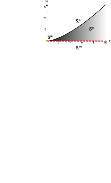
Figure 8: Orbit space and symmetry strata of the (SO${}_{3}\times{\mathbb{Z}}_{2}$, ${\underline{5}})$ gauge model.

By selecting a convenient point ($\phi_{1}=\phi_{2}=\phi_{3}=0$) in an arbitrarily chosen orbit in each of the primary strata, and determining the corresponding isotropy subgroup, one easily finds that the primary strata coincide with symmetry strata. Their residual symmetries are: [SO${}_{3}\times{\mathbb{Z}}_{2}$], [SO₂], $[{\mathbb{Z}}_{2}]$ and $[1\!\!1]$, respectively for $S^{(0)}$, $S^{(1)}_{1}$, $S^{(1)}_{2}$ and $S^{(2)}$. Let us describe the details of the calculation only in the case of the new phase associated to the stratum $S^{(1)}_{2}$.

For $\phi_{1}=\phi_{2}=\phi_{3}=0$, the condition $p_{2}(\phi)=0$ reduces to $\phi_{5}(3\phi_{4}^{2}-\phi_{5}^{2})=0$. It is sufficient to take into consideration only one of the solutions of this condition, since, for fixed values of $p_{1}(\phi)=\phi^{2}_{4}+\phi^{2}_{5}$, the other solutions lie on the same orbit and variations of $p_{1}$ lead to orbits of the same stratum. The solution $\phi_{5}=0$ corresponds to a matrix

$$\Phi_{0}=\frac{1}{\sqrt{2}}\,\left(\begin{array}[]{ccc}\phi_{4}&0&0\\ 0&-\phi_{4}&0\\ 0&0&0\end{array}\right),$$ (27)

which is invariant only under the transformations of the “parity” subgroup ${\mathbb{Z}}^{\prime}_{2}$ of SO${}_{3}\times{\mathbb{Z}}_{2}$ generated by the transformation resulting from a parity transformation $\phi\rightarrow-\phi$, followed by an SO₃ transformation, generated by the matrix

$$\gamma=\left(\begin{array}[]{ccc}0&-1&0\\ -1&0&0\\ 0&0&-1\end{array}\right)\,,$$ (28)

that exchanges the two non trivial elements of $\Phi_{0}$.

In a renormalizable version of the model, the Higgs potential can be written in the form of (4), (5), with $a_{2}=0$ (a choice that, in this case, is rigorously required by the symmetry of the model), and $a_{3}>0$, to guarantee that the potential is bounded from below.

In this model, the potential $\widehat{V}(p)$ is independent of $p_{2}$. As a consequence, in the $p$-space, equipotential lines reduce to straight-lines $p_{1}=c=$const. It is, therefore, clear that, for $a_{1}>0$, $\widehat{V}(p)$ has a stable minimum at $p_{1}=0=p_{2}$ ($c=0$), while for $a_{1}<0$ its minimum is degenerate along the straight-line $p_{1}=-a_{1}/a_{3}$, which crosses all the strata, but for $S^{(0)}$. As a consequence, the minimum is unstable and only the phase ${\mathcal{F}}^{(0)}$ is observable at tree-level.

If one gives up renormalizability and allows Higgs potentials of arbitrarily high degree, then it would be easy to show, arguing as in the preceding subsection, that at degree six also the phases ${\mathcal{F}}^{(1)}_{1}$ and ${\mathcal{F}}^{(1)}_{2}$ become tree-level observable, while degree twelve (the degree of ${p}_{2}^{2}(\phi)$) has to be reached in order to make sure that all the allowed phases are tree-level observable.

The dominant one-loop radiative corrections $V_{\rm g}$ are the same calculated in the case of the SO₃ model. As emphasized in CW and recalled in the preceding subsection, for $a_{1}<0$ they constrain the minimum of the effective potential in the stratum $S^{(1)}_{1}$ (${p}_{2}={p}_{1}^{3}$), with symmetry [SO₂], and the minimum is stable. Thus, at one-loop, the phase ${\mathcal{F}}^{(1)}_{2}$ is observable, but it is clear that ${\mathcal{F}}^{(1)}_{2}$ and ${\mathcal{F}}^{(2)}$ remain unobservable.

The results we have found are in complete agreement with the results in CW, but a comparison of the SO₃ and the SO${}_{3}\times{\mathbb{Z}}_{2}$ models makes it difficult for us to share the enthusiasm manifested by CW for the fact that in the SO${}_{3}\times{\mathbb{Z}}_{2}$ model “there is nothing in the symmetry properties of this theory that guarantees that the minimum of $V$ will obey Eq.(6,18). Thus, …, if a massless photon emerges, it will be as a consequence of detailed dynamics, not just of trivial group theory.” In fact, in the (SO₃, ${\underline{5}}$) model, which has the same gauge group, the emergence of a massless photon can be stated already at tree-level: it is a consequence of trivial group theory. In the SO${}_{3}\times{\mathbb{Z}}_{2}$ model, the exceeding degeneracy of the absolute minimum of the Higgs potential, which prevents the choice of the true vacuum at tree-level, is an artifact due to the combined effects of the additional discrete symmetry ${\mathbb{Z}}_{2}$ and the limit imposed by renormalizability on the degree of the Higgs potential. The introduction of the additional discrete reflection symmetry, justified in CW “to simplify the problem”, does, indeed, strongly modify the symmetry of the model and its allowed and observable phases: a new allowed phase is generated and the allowed phase with symmetry [SO₂] is made unobservable at tree-level. Discrete symmetries play important roles, not only from the phenomenological point of view and in the characterization of the allowed phases, but also in the selection of the observable ones.

2.2 An (SU₃, 8) gauge model

Let us consider a model with gauge group SU₃ and an octet $\phi$ of real Higgs fields, transforming as a vector in the space of the adjoint representation of the group. Like in the models studied above, the linear group $G=$(SU₃, ${\underline{8}}$) admits only two basic homogeneous invariant polynomials, that can be conveniently chosen to be the following:

$$p_{1}(\phi)=\sum_{i=1}^{8}\,\phi_{i}^{2},\hskip 25.0ptp_{2}(\phi)=\sqrt{3}\,\sum_{i,j,k=1}^{8}\,d_{ijk}\phi_{i}\,\phi_{j}\,\phi_{k},$$ (29)

where the $d_{ijk}$ is the usual completely symmetric Gell-Mann [26] tensor. The Higgs potential can be written, in terms of the basic invariants $p=(p_{1},p_{2})$ defined in (29) as in (4), (5). The $\widehat{P}(p)$-matrix and, therefore, the orbit space, turns out to be isomorphic to the orbit space of the linear group (SO₃, ${\underline{5}}$).

Therefore, the geometric aspects of the minimization problem, both in the renormalizable version of the model and in a non-renormalizable one, with a Higgs potential of degree six, are exactly the same solved in the case of the (SO₃, ${\underline{5}})$ model.

Only the symmetries of the four primary strata have to be recalculated in the model we are discussing. As well known they are [SU₃] (stratum $S^{(0)}=W^{(0)}$), [SU${}_{2}\times\mathrm{U}_{1}$] (stratum $S^{(1)}=W^{(1)}_{1}\cup W^{(1)}_{2}$), [$\mathrm{U}_{1}\times\mathrm{U}_{1}$] (stratum $S^{(2)}=W^{(2)}$), respectively. Also in this case there are three allowed phases and only ${\mathcal{F}}^{(0)}$ and ${\mathcal{F}}^{(1)}$ turn out to be tree-level observable in a renormalizable version of the model, while all the allowed phases are tree level observable if a non-renormalizable Higgs potential of degree six is allowed.

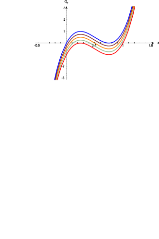
Figure 9: Family of functions $q^{\prime}_{\eta}(z)$, in the interval $[0,1]$, for $\eta=0,\;1/4,\;1/2,\;3/4,\;1$.

Figure 10: Graph of the function $f(\eta)=\sum_{i=1}^{3}z_{i}^{2}(\eta)\mathrm{ln}\left(z_{i}(\eta)\right)$, where $z_{i}(\eta)$ are the roots of the polynomial $q^{\prime}_{\eta}(z)$ .

As for the one-loop radiative corrections due to the vector bosons, the explicit form of $V_{\rm g}$ is given in (18), where

$${M_{ab}^{2}(\phi)=g^{2}\,\langle F_{a}\phi,F_{b}\phi\rangle,\hskip 25.0ptF_{a,ij}=f_{aij},\hskip 25.0pta,i,j=1,\dots,8}$$ (30)

and the $f_{aij}$ are the usual SU₃ completely antisymmetric structure constants.

The squared mass matrix $M^{2}$ has three non zero distinct eigenvalues that, also in this case, are algebraic $G$-invariant functions of $\phi$.

The same procedure followed in the case of the SO₃ model, allows to express them in the form $p_{1}\,z_{i}$, where the $z_{i}$’s are the roots of the following polynomial in $z$:

$${q^{\prime}_{\eta}(z)=(-1+z)(-1+4\,z)^{2}+\eta\,,\quad\eta=\dfrac{p_{2}^{2}}{p_{1}^{3}}.}$$ (31)

The range of the adimensional variable $\eta$ is the interval $[0,1]$. The polynomial functions $q^{\prime}_{\eta}(z)$ are plotted, for different values of $\eta$, in Fig. 10 and $V_{\rm g}$ as a function of $\eta$ is plotted in Fig. 10, for fixed values of $p_{1}$. The contribution $V_{\rm g}$ to the one-loop radiative corrections has evidently an absolute minimum for $\eta=1$. We conclude, therefore, that, like in the case of the SO₃ model, one-loop radiative corrections are not sufficient to make observable the phase ${\mathcal{F}}^{(2)}$ (not observable at tree-level).

3 The geometrical invariant theory approach to spontaneous symmetry breaking

The approach followed in the previous section to determine all the allowed phases in a gauge model can be formulated on an absolutely general and rigorous ground [22, 23, 5]. Let us briefly recall the basic elements.

Let $\phi$ denote the set of real scalar fields of the model to be thought of as a vector $\phi\in{\mathbb{R}}^{n}$ (vector order parameter), transforming according to a real orthogonal representation of the gauge group: $\phi\rightarrow g\cdot\phi$. We shall denote by $G$ the group of real orthogonal $n\times n$ matrices $g$.

The Higgs potential $V^{(d)}_{a}(\phi)$ is a $G$-invariant real polynomial function of $\phi$ with real coefficients $a_{i}$ (control parameters) and degree $d$. The observable phases of the system are determined by the location of the points of stable global minimum of $V^{(d)}_{a}(\phi)$. Owing to $G$-invariance, the Higgs potential is a constant along each $G$-orbit, so, each of its stationary points is degenerate along a whole $G$-orbit. Minima lying on the same $G$-orbit define equivalent vacua. Since the isotropy subgroups $G_{\phi}$ of $G$ at points $\phi$ of the same $G$-orbit are conjugate in $G$ ($G_{g\phi}=g\,G_{\phi}\,g^{-1}$), only the conjugacy class $[G_{\phi}]=\{g\,G_{\phi}\,g^{-1}\mid\,g\in G\}$ formed by the isotropy subgroups of $G$ at the points of the orbit of minima, i.e. the symmetry or orbit-type of the orbit hosting the absolute minimum, is physically relevant, and defines the symmetry of the associated stable phase.

The set of all $G$-orbits, endowed with the quotient topology and differentiable structure, forms the orbit space, ${\mathbb{R}}^{n}/G$, of $G$. The subset of all the points lying in $G$-orbits of the same orbit-type forms a symmetry stratum of ${\mathbb{R}}^{n}$ and the image in the orbit space of a symmetry stratum of ${\mathbb{R}}^{n}$ forms a stratum of ${\mathbb{R}}^{n}/G$. Phase transitions take place when, by varying the values of the control parameters, the absolute minimum of $V^{(d)}_{a}(\phi)$ is shifted to an orbit lying on a different stratum.

If $V^{(d)}_{a}(\phi)$ is a polynomial in $\phi$ of sufficiently high degree, by varying the control parameters, its absolute minimum can be shifted to any stratum of ${\mathbb{R}}^{n}/G$. So, the strata are in a one-to-one correspondence with the allowed phases. On the contrary, extra restrictions on the form of the Higgs potential, not coming from G-symmetry requirements (e.g., the assumption that it is a polynomial of degree $\leq 4$ in the Higgs fields), can prevent its global minimum from sitting, as a stable (against perturbations of the control parameters) minimum, in particular strata and make, consequently, the corresponding allowed phases dynamically unattainable at tree-level.

Being constant along each $G$-orbit, the Higgs potential can be conveniently thought of as a function defined in the orbit space ${\mathbb{R}}^{n}/G$ of $G$. This fact can be formalized using some basic results of invariant theory. In fact, every $G$-invariant polynomial function $F(\phi)$ can be built as a real polynomial function $\widehat{F}(p)$ of a finite set, $\{p_{1}(\phi),\dots,p_{q}(\phi)\}$, of basic homogeneous polynomial invariants (minimal integrity basis of the ring ${\mathbb{R}}\left[{\mathbb{R}}^{n}\right]^{G}$ of $G$-invariant polynomials, hereafter abbreviated in MIB) [27]:

$${F(\phi)=\widehat{F}(p(\phi)),\quad\phi\in{\mathbb{R}}^{n}}$$ (32)

and the range $p({\mathbb{R}}^{n})$ of the orbit map, $\phi\mapsto p(\phi)=(p_{1}(\phi),\dots,p_{q}(\phi))$ yields a diffeomorphic realization of the orbit space of $G$, as a connected semi-algebraic set in ${\mathbb{R}}^{q}$, i.e., as a subset of ${\mathbb{R}}^{q}$, determined by algebraic equations and inequalities. Thus, the elements of an integrity basis can be conveniently used to parametrize the points of $p({\mathbb{R}}^{n})$ that, hereafter, will be identified with the orbit space ${\mathbb{R}}^{n}/G$.

The elements of a minimal integrity basis need not, for general compact groups, be algebraically independent. If they are not so, the linear group $G$ is said to be non-coregular and the algebraic relations among the elements of its MIB’s are called syzygies. The number $q_{0}$ of algebraically independent elements in a MIB is $n-{\rm Dim}(\Omega_{\rm p})$, where ${\rm Dim}(\Omega_{\rm p})$ is the dimension shared by all the generic (principal) orbits $\Omega_{\rm p}$ of $G$. The linear groups studied in the preceding section are all coregular. Examples of non coregular groups will be met in the second part of the paper.

The orbit space of $G$ presents a natural geometric stratification, like all semi-algebraic sets. It can, in fact, be considered as the disjoint union of a finite number of connected semi-algebraic subsets of decreasing dimensions (primary strata), each primary stratum being a connected manifold open in its topological closure and lying in the boundary of a higher dimensional one (but for the highest dimensional stratum, which is unique and called principal stratum). The primary strata are the connected components of the symmetry strata. All the connected components of a symmetry stratum have the same dimension and the symmetries of two bordering symmetry strata are related by a group–subgroup relation, the orbit-type of the lower dimensional stratum being larger: more peripheric strata have larger symmetries.

If the only $G$-invariant point of ${\mathbb{R}}^{n}$ is the origin, there are no linear invariants and in ${\mathbb{R}}^{n}/G$ there is only one 0-dimensional stratum, corresponding to the origin of ${\mathbb{R}}^{q}$. All the other strata have at least dimension 1, since the isotropy subgroups of $G$ at the points $\phi\in{\mathbb{R}}^{n}$ and $\lambda\,\phi$, $\lambda\in{\mathbb{R}}$, are equal and, therefore, the points $(p_{1},\dots,p_{q})$ and $(\lambda^{d_{1}}p_{1},\dots,\lambda^{d_{q}}p_{q})$ ($d_{i}$ the degree of the basic invariant $p_{i}(\phi)$) sit on the same stratum. This fact, added to the homogeneity of the basic invariants and of the relations defining the strata, shows also that a complete information on the structure of the orbit space and its stratification can be obtained from its intersection with the image in ${\mathbb{R}}^{n}/G$ of the unit sphere of ${\mathbb{R}}^{n}$.

The semialgebraic set $p({\mathbb{R}}^{n})$, yielding an image of the orbit space of $G$ in the $p$-space, and its stratification has been shown to be determined by the points $p\in{\mathbb{R}}^{q}$, satisfying the following conditions [22, 23, 5]:

Theorem 1

Let $G$ be a compact linear group acting in ${\mathbb{R}}^{n}$, $\{p_{1}(\phi),\dots,p_{q}(\phi)\}$ a MIB of ${\mathbb{R}}\left[{\mathbb{R}}^{n}\right]^{G}$ and $Z\subseteq{\mathbb{R}}^{q}$ the algebraic variety of the relations among the $p_{i}(\phi)$’s. Then, $p({\mathbb{R}}^{n})$ is the unique connected semi-algebraic subset of $Z$ where the matrix $\widehat{P}(p)$, defined by the following relations, is positive semi-definite:

$$\widehat{P}_{ab}(p(\phi))=\sum_{j=1}^{n}\partial_{j}p_{a}(\phi)\,\partial_{j}p_{b}(\phi),\hskip 25.0pt\phi\in{\mathbb{R}}^{n}\,,\quad a=b=1,\,\ldots,\,q.$$ (33)

The $k$-dimensional primary strata of $p({\mathbb{R}}^{n})$ are the connected components of the set $\widehat{W}^{(k)}=\{p\in{\mathbb{R}}^{q}\mid\widehat{P}(p)\geq 0,\ {\rm rank\,}\widehat{P}(p)=k\}$; they are the images of the connected components of the $k$-dimensional isotropy type strata of ${\mathbb{R}}^{n}/G$. In particular, the set of the interior points of $p({\mathbb{R}}^{n})$ is the image of the principal stratum.

In the following, the primary and symmetry strata will always be denoted by $W^{(i)}_{j}$ and $S^{(i)}_{k}$ respectively, where the apex $i$ gives the dimension of the stratum and $j$ or $k$ are order numbers, which will be omitted if not necessary.

There is always at least a $G$-invariant polynomial of degree two, that, in this section, we shall denote by $p_{1}$:

$${p_{1}(\phi)=\sum_{i=1}^{n}\,\phi_{i}^{2}.}$$ (34)

With this convention, $\partial p_{1}(\phi)=2\phi_{i}$, so that the first row and column of the matrix $\widehat{P}(p)$ are completely determined to be $P_{1i}(p)=P_{i1}(p)=2d_{i}\,p_{i}$ by Euler equation, owing to the homogeneity of the polynomials $p_{i}(\phi)$. Moreover, the image in orbit space of a sphere of ${\mathbb{R}}^{n}$, centered in the origin, is the intersection of the orbit space with the linear variety of equation $p_{1}=$ const. This intersection is necessarily a compact subset, so any continuous function of $p$ certainly has an absolute minimum for a fixed value of $p_{1}$.

By defining, according to (32),

$$\widehat{V}^{(d)}_{a}(p(\phi))=V^{(d)}_{a}(\phi),\hskip 25.0pt\phi\in{\mathbb{R}}^{n},$$ (35)

the range of $V^{(d)}_{a}(\phi)$ coincides with the range of the restriction of $\widehat{V}^{(d)}_{a}(p)$ to the the orbit space $p({\mathbb{R}}^{n})$ and the local minima of $V^{(d)}_{a}(\phi)$ can be computed as the local minima of the function $\widehat{V}^{(d)}_{a}(p)$ with domain $p({\mathbb{R}}^{n})$.

In detail, denoting by $f_{\alpha}(p)=0$, $\alpha=1,\dots k$ a complete set of independent equations of the stratum $S$, the conditions for the occurrence of a stationary point of the potential at $p\in S$, can be conveniently written in the following form:

$${\left\{\begin{array}[]{l}f_{\alpha}(p)=0,\hskip 25.0pt\alpha=1,\dots,k,\\ \dfrac{\partial}{\partial p_{i}}\left(\widehat{V}^{(d)}_{a}(p)-\sum_{\alpha=1}^{k}\,\lambda_{\alpha}\,f_{\alpha}(p)\right)=0,\hskip 25.0pti=1,\dots,q,\end{array}\right.}$$ (36)

where the $\lambda_{\alpha}$’s are real Lagrange multipliers. A stationary point at $\overline{p}$ will be a stable local minimum on the stratum if the Hessian matrix $M^{2}_{\rm s}(\phi)$ of $V^{(d)}_{a}(\phi)$ is $\geq 0$ and has rank $n$ minus the dimension $\nu$ of the orbit ($\nu$ equals the number of Goldstone bosons), for any $\phi$ lying on the orbit of equation $p(\phi)=\overline{p}$. These conditions can be conveniently expressed in terms of the sums $K_{i}$ of the (determinants of) the principal minors of $M^{2}_{\rm s}(\phi)$ in the form $K_{i}>0$, $i=1,\dots,n-\nu$. Being $M^{2}_{\rm s}(\phi)$ a $G$-tensor of rank 2, the $K_{i}$’s are $G$-invariant polynomials in the $\phi_{i}$’s and can, therefore be expressed as polynomials in the elements of the MIB. As shown in [5, 23], the squared mass matrix of the scalars is reducible in the singular strata, so the above conditions on its semi-positivity and rank are equivalent to the following simpler conditions (for any $\phi$ on the $G$-orbit of equation $p(\phi)=\overline{p}$:

1. the $n\times n$ matrix $\partial^{2}(V^{(d)}_{a}(\phi)-\sum_{\alpha=1}^{k}\,\lambda_{\alpha}\,f_{\alpha}(p(\phi)))/\partial\phi_{i}\partial\phi_{j}$ is $\geq 0$ and its rank equals the dimensions $q-k$ of $S$;

2. the $n\times n$ matrix $\partial^{2}(\sum_{\alpha=1}^{k}\,\lambda_{\alpha}\,f_{\alpha}(p(\phi)))/\partial\phi_{i}\partial\phi_{j}$ is $\geq 0$ and its rank equals the dimension $n-(q-k)-\nu$ of the orthogonal space in ${\mathbb{R}}^{n}$ to the stratum at $\phi)$).

Also these conditions can obviously be expressed in terms of the principal minors of the matrices, i.e. as polynomial inequalities in the basic invariants. The requirement for $V_{a}^{(d)}(\phi)$ being bounded from below is equivalent to the condition that the constrained minimum of $V_{a}^{(d)}(\phi)$, in the intersection of the orbit space with the hyperplane of equation $p_{1}=$ const ($p_{1}$ is defined in (34)), is positive.

4 Allowed and observable phases in some two-Higgs doublet extensions of the Standard Model

The possibility of generating the observed Baryon Asymmetry of our Universe (BAU) during the Electro-Weak Phase Transition (EWPT) has been extensively studied since the middle of the eighties by several authors (see for instance [28, 29] and references therein). It is nowadays well established that the Standard Model is not suited to account for BAU, both because the amount of CP violation in the quark sector is too tiny and because the experimental lower bounds on the Higgs mass cause the phase transition not being enough strongly first order to prevent the baryon excess generated at the EWPT from being subsequently washed out by sphaleron effects. In the 2HD models there is a natural additional source of CP violation: the phase between the two VEV’s of the Higgs fields. Notwithstanding, as was pointed out in [29], since the baryon production ceases at very small values of the Higgs fields, models with only two Higgs doublets can hardly generate the right amount of BAU, because at the EWPT they behave as models with one light Higgs doublet, with the second heavier Higgs decoupling and having small impact on the phase transition. More promising has been the introduction of gauge singlet scalars which couple to the Higgs. In particular, a model with a second Higgs doublet and a complex gauge singlet has been analyzed in connection with baryogenesis and the dark matter problem in [30].

In this section, we shall characterize all the allowed and tree-level observable phases and all possible phase transitions between contiguous phases, for variants of a 2HD extension of the SM. In particular, for each model we shall determine a minimal set of basic polynomial invariants of $G$, the geometrical features of the orbit space, i.e. its stratification (including connectivity properties and bordering relations of the strata) and the orbit-types of its strata. Since our analysis will be stricly bounded to tree-level Higgs potentials, all our statements will be intended as tree-level statements, even when not explicitly claimed.

The conclusion will be that, if discrete symmetries are added, the renormalizable versions of the models are incomplete. In the following section we shall show that renormalizability and completeness can be reconciled if these models are extended by adding convenient scalar singlets.

4.1 Model 0: The two-Higgs extension of the Standard Model

In this subsection we analyze the basic two-Higgs extension of the Standard Model. The symmetry group of the Lagrangian is SU${}_{2}\times\mathrm{U}_{1}$ and there are two complex Higgs doublets $\Phi_{1}$ and $\Phi_{2}$ of hypercharge $Y=1$:

$${\Phi_{1}=\left(\begin{array}[]{c}\phi_{1}+i\,\phi_{2}\\ \phi_{3}+i\,\phi_{4}\end{array}\right)\,,\hskip 25.0pt\Phi_{2}=\left(\begin{array}[]{c}\phi_{5}+i\,\phi_{6}\\ \phi_{7}+i\,\phi_{8}\end{array}\right)\,,\hskip 25.0pt\phi_{i}\in{\mathbb{R}}.}$$ (37)

In this model, natural flavor conservation is violated by neutral current effects in the phase (hereafter called ${\mathcal{F}}^{(3)}$), that should correspond to the present phase of our Universe. So the model is not realistic, but it provides a simple example in which renormalizability does not exclude completeness.

The transformation induced by the element $\hat{j}=(-1\!\!1_{2},\mathrm{e}^{\mathrm{i}\pi Y})\in$ SU${}_{2}\times\mathrm{U}_{1}$ leaves invariant the fields $\Phi_{1}$ and $\Phi_{2}$. So, the linear group acting on the vector $\phi=(\phi_{1},\dots,\phi_{8})$ of the real Higgs fields of the model is $G=\left((\mathrm{SU}_{2}\times\mathrm{U}(1))/{\mathbb{Z}}_{2},\ {\underline{8}}\right)$, where ${\mathbb{Z}}_{2}$ is the group generated by $\hat{j}$.

A convenient choice for a MIB of real independent polynomial $G$-invariants is the following:

$${p_{1}=\Phi_{1}^{\dagger}\Phi_{1}+\Phi_{2}^{\dagger}\Phi_{2},\ \ p_{2}=\Phi_{1}^{\dagger}\Phi_{1}-\Phi_{2}^{\dagger}\Phi_{2},\ \ p_{3}+ip_{4}=2\,\Phi_{2}^{\dagger}\Phi_{1}.}$$ (38)

The relations defining $p({\mathbb{R}}^{4})$ and its strata, which are listed in Table 1, can be obtained from rank and positivity conditions of the $\widehat{P}(p)$-matrix associated to the MIB defined in Eq. (38):

$${\widehat{P}(p)=\left(\begin{array}[]{cccc}4\,p_{1}&4\,p_{2}&4\,p_{3}&4\,p_{4}\\ 4\,p_{2}&4\,p_{1}&0&0\\ 4\,p_{3}&0&4\,p_{1}&0\\ 4\,p_{4}&0&0&4\,p_{1}\end{array}\right)\,.}$$ (39)

Stratum	Defining relations	Symmetry	Boundary	Typical point $\phi$
$S^{(4)}$	$p_{1}>\sqrt{p_{2}^{2}+p_{3}^{2}+p_{4}^{2}}$	$\{1\!\!1\}$	${\overline{S}}^{(3)}$	$(\phi_{1},0,\phi_{3},\phi_{4},0,0,\phi_{7},0)$
$S^{(3)}$	$p_{1}=\sqrt{p_{2}^{2}+p_{3}^{2}+p_{4}^{2}}$	U${}_{1}^{\mathrm{e}.m.}$	$S^{(0)}$	$(0,0,\phi_{3},\phi_{4},0,0,\phi_{7},0)$
$S^{(0)}$	$p_{1}=p_{2}=p_{3}=p_{4}=0$	$G$		$(0,0,0,0,0,0,0,0)$

Table 1: Strata of the orbit space for the symmetry group $G=(\mathrm{SU}_{2}\times\mathrm{U}_{1})/{\mathbb{Z}}_{2}$ of Model 0. A bar denotes topological closure. The group U${}_{1}^{\mathrm{e}.m.}$ is formed by the elements $\left\{\mathrm{e}^{\mathrm{i}\theta(T_{3}+Y/2)}\right\}_{0\leq\theta<2\pi}$. For each stratum, a field configuration with the same symmetry is supplied (typical point). The $\phi_{i}$’s are generic non zero values.

The orbit space is the half-cone bounded by the surface of equation $p_{1}=\sqrt{\sum_{i=2}^{4}p_{i}^{2}}$. There are, evidently, only three primary strata of dimensions 0, 3 and 4. They are connected sets and have, consequently, to be identified to the three distinct symmetry strata: the tip of the cone corresponds to the stratum $S^{(0)}$, and the rest of the surface to the stratum $S^{(3)}$, while the interior points form $S^{(4)}$. There are no one-dimensional and two-dimensional strata.

A general fourth-degree polynomial invariant Higgs potential can be written in the following form:

$$\begin{array}[]{rcl}\widehat{V}(p)&=&\sum_{i,j=1}^{4}\,A_{ij}\,p_{i}\,p_{j}+\sum_{i=1}^{4}\,\alpha_{i}\,p_{i}\\ &&\\ &=&\sum_{i,j=1}^{4}\,A_{ij}\,(p_{i}-\eta_{i})(p_{j}-\eta_{j})-\sum_{i,j=1}^{4}\,A_{ij}\,\eta_{i}\,\eta_{j},\end{array}$$ (40)

where, to make sure that $\widehat{V}(p)$ is bounded from below, we assume that all the coefficients are real and the symmetric matrix $A$ is positive definite. Moreover: $\eta_{i}=-\frac{1}{2}\sum_{j=1}^{4}(A^{-1})_{ij}\,\alpha_{j}$.

In this simple case (convex orbit space), the constrained minima of $\widehat{V}(p)$ can be easily determined from elementary geometrical considerations. To this end, let us first choose $A\propto 1\!\!1$ and let us denote by $C=C^{+}\cup C^{-}$ the closed double cone bounded by the surfaces of equation $p_{1}=\pm\sqrt{\sum_{i=2}^{4}p_{i}^{2}}$ in the $p$-space ${\mathbb{R}}^{4}$. Then, since the potential is a constant plus the squared distance of $p$ from $\eta$, for given values of the $\eta_{i}$’s, the potential has a stable absolute minimum at the point $p$ of the orbit space which is closest to $\eta$. One is left, therefore, with the following possibilities:

• the minimum is stable in $S^{(4)}$, at $p=\eta$, for $\eta$ in the interior of $C^{+}$;

• the minimum is stable in $S^{(0)}$ ($p=0$) for $\eta$ in the interior of $C^{-}$;

• the minimum is stable in $S^{(3)}$, at the nearest point to $\eta$, for $\eta$ outside $C$;

• the minimum is unstable in $S^{(3)}\cup S^{(0)}$, at $p=\eta$, for $\eta$ on the surface of the double cone.

For a general fixed $A>0$, the results do not essentially change, since one can revert to the case $A=1\!\!1$ by means of a convenient linear transformation of the $p_{i}$’s, which defines a new (equivalent) MIB: as a result, $C^{+}$ and $C^{-}$ are simply rotated and deformed by independent re-scalings along the coordinate axes. So, in the space of the parameters $(\alpha_{1},\dots,\alpha_{4})$, that are independent linear combinations of the $\eta_{i}$’s, there are three disjoint open regions of stability of the three allowed phases associated to the strata of the orbit space. These regions are separated by inter-phase boundaries, formed by critical points where second order phase transitions may start; moreover, first order phase transitions cannot take place.

We can conclude that the model just discussed is both renormalizable and (tree-level) complete.

4.2 Model 1: A FCNC protecting version of Model 0

The model we shall analyze in this subsection contains the same set of fields as Model 1, but a discrete symmetry, generated by a reflection $\hat{\iota}$ is added, to protect the theory from FCNC processes (see, for instance [14, 15] and references therein). So, the symmetry group of the Lagrangian is assumed to be SU${}_{2}\times\mathrm{U}_{1}\times\{\hat{\iota}\}$, where $\{\hat{\iota}\}$ denotes the ${\mathbb{Z}}_{2}$ group generated by $\hat{\iota}$, which is assumed to act on the Higgs fields in the following way: $(\Phi_{1},\Phi_{2})\rightarrow(\Phi_{1},-\Phi_{2})$.

The phase transitions of Model 1 have been analyzed in [12, 13]. The possibility of two–stage phase transitions was proposed in [12] to reconcile the smallness of the CP-breaking term explicitly introduced at tree-level and the necessary amount of CP violation required to successfully account for baryogenesis. The author asserts that “Investigating the whole parameter space would be too time consuming”, so he performs only a numerical analysis of the nature of the phase transition driven by the third degree finite temperature corrections to the classical potential. In a more recent paper [13], the full contribution of the extra breaking terms (not considering them as perturbations) is also examined. The result is still a two–stage phase transition, but, in addition to the CP violation, the phase transition to the charge conserving vacuum generates some charge asymmetry in the presence of heavy leptons, which is compared with the astrophysical bounds.

The orbit space approach enables us to study such problems analytically and in full generality. Moreover, in an extended renormalizable and complete version of Model 1, Model 1C, that we shall study in a subsequent subsection, we shall check the possibility of spontaneous CP violation [31].

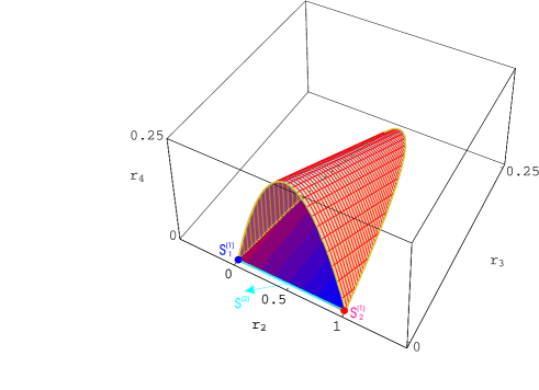
Figure 11: Representation in ${\mathbb{R}}^{3}$ of the section $\Xi$ of one of the two layers $p_{5}=\pm\sqrt{p_{3}p_{4}}$ of the four dimensional orbit space of Model 1 with the hyperplane of equation $p_{1}+p_{2}=1$. In this representation the primary stratification cannot be deduced directly from the figure. The blue and red points represent the one dimensional strata $S^{(1)}_{1}$ and $S^{(1)}_{2}$, respectively. They are connected by a pale blue line representing the stratum $S^{(2)}$. $\Xi$ looks like a cave: the union of the entrance, the floor and the interior form the principal stratum $S^{(4)}$, while the union of the ceiling and its green border represents the stratum $S^{(3)}$. The relations defining the strata can be found in Table 2.

${S}$	Defining relations	Symmetry	Boundary	Typical point $\phi$
${S}^{(4)}$	${p}_{5}^{2}-{p}_{3}{p}_{4}=0$	$\{1\!\!1\}$	$\overline{{S}^{(3)}}\,,\;\overline{{S}^{(2)}}$	$(\phi_{1},0,\phi_{3},\phi_{4},0,0,\phi_{7},0)$
	${p}_{1}+{p}_{2}>0\,,\;$
	${p}_{3}+{p}_{4}>0\,,\;$
	${p}_{1}{p}_{2}-{p}_{3}-{p}_{4}>0$
${S}^{(3)}$	${p}_{5}^{2}-{p}_{3}{p}_{4}=0\,,$	U${}_{1}^{\rm e.m.}$	$\overline{{S}^{(1)}_{1}}\,,\;\overline{{S}^{(1)}_{2}}$	$(0,0,\phi_{3},\phi_{4},0,0,\phi_{7},0)$
	${p}_{1}{p}_{2}-{p}_{3}-{p}_{4}=0\;$
	${p}_{1}\,,{p}_{2}>0\,,$
	${p}_{3},\,{p}_{4}\geq 0$
${S}^{(2)}$	${p}_{j}=0\,,\;j\neq 1,2$	$\{\alpha\hat{i}\}$	$\overline{{S}^{(1)}_{1}}\,,\;\overline{{S}^{(1)}_{2}}$	$(\phi_{1},0,0,0,0,0,\phi_{7},0)$
	${p}_{1}\,,{p}_{2}>0\;$
${S}^{(1)}_{1}$	${p}_{j}=0<{p}_{1}\,,\;j\neq 1$	U${}_{1}^{\rm e.m.}\times\{\hat{\iota}\}$	${S}^{(0)}$	$(0,0,\phi_{3},0,0,0,0,0)$
${S}^{(1)}_{2}$	${p}_{j}=0<{p}_{2}\,,\;\;j\neq 2\;$	U${}_{1}^{\rm e.m.}\times\{e^{i\pi Y}\,\hat{\iota}\}$	${S}^{(0)}$	$(0,0,0,0,0,0,\phi_{7},0)$
${S}^{(0)}$	${p}_{i}=0\,,$ $1\leq i\leq 5$	$G$		$(0,0,0,0,0,0,0,0)$

Table 2: Strata $S$ of the orbit space for the symmetry group $G=(\mathrm{SU}_{2}\times$U${}_{1})/{\mathbb{Z}}_{2}\times\{\hat{\iota}\}$ of Model 1. A bar denotes topological closure. The group U${}_{1}^{\rm e.m.}$ is formed by the elements $\left\{e^{i\theta(T_{3}+Y/2)}\right\}_{0\leq\theta<2\pi}$. For each stratum, a field configuration with the same symmetry is supplied (typical point). The $\phi_{i}$’s are generic non zero values. Confining strata are indicated, so that possible second order phase transitions can be easily identified.

In Model 1, the linear group acting on the vector $\phi$ of real Higgs fields is $G=\left((\mathrm{SU}_{2}\times\mathrm{U}(1))/{\mathbb{Z}}_{2}\,\times\{\hat{\iota}\},\ \underline{8}\right)$ and a MIB is the following:

$$\begin{array}[]{l}{p}_{1}=\Phi_{1}^{\dagger}\Phi_{1},\;\;{p}_{2}=\Phi_{2}^{\dagger}\Phi_{2},\;\;{p}_{3}=\left(\mathrm{Re}\left[\Phi_{2}^{\dagger}\Phi_{1}\right]\right)^{2},\\ \\ {p}_{4}=\left(\mathrm{Im}\left[\Phi_{2}^{\dagger}\Phi_{1}\right]\right)^{2},\;\;{p}_{5}=\mathrm{Re}\left[\Phi_{2}^{\dagger}\Phi_{1}\right]\;\mathrm{Im}\left[\Phi_{2}^{\dagger}\Phi_{1}\right].\end{array}$$ (41)

The elements of the MIB are related by a syzygy $s=p_{5}^{2}-p_{3}\,p_{4}$, so the orbit space is the four dimensional algebraic variety of equation $s=0$ in the 5–dimensional $p$-space. The defining relations of the strata of ${p}({\mathbb{R}}^{8})$, summarized in Table 2, are obtained from positivity and rank conditions of the matrix $\widehat{P}({p})$, associated to the MIB of Eq. (41):

$${\widehat{P}(p)=\left(\begin{array}[]{ccccc}4{p}_{1}&0&4{p}_{3}&4{p}_{4}&4{p}_{5}\\ 0&4{p}_{2}&4{p}_{3}&4{p}_{4}&4{p}_{5}\\ 4{p}_{3}&4{p}_{3}&4{p}_{3}\,({p}_{1}+{p}_{2})&0&2{p}_{5}\,({p}_{1}+{p}_{2})\\ 4{p}_{4}&4{p}_{4}&0&4{p}_{4}\,({p}_{1}+{p}_{2})&2{p}_{5}\,({p}_{1}+{p}_{2})\\ 4{p}_{5}&4{p}_{5}&2{p}_{5}\,({p}_{1}+{p}_{2})&2{p}_{5}\,({p}_{1}+{p}_{2})&({p}_{1}+{p}_{2})\,({p}_{3}+{p}_{4})\end{array}\right)}$$ (42)

The orbit space $p({\mathbb{R}}^{8})\subset{\mathbb{R}}^{5}$ is formed by the union of two layers of equations $p_{5}=\pm\sqrt{p_{3}p_{4}}$. The intersections with the hyperplane of equation ${p}_{1}+{p}_{2}=1$ are isomorphic and can be represented, in a three dimensional space, as the closed solid (semialgebraic set) $\Xi$ shown in Figure 11. The full orbit space is the four dimensional connected semi-algebraic set of ${\mathbb{R}}^{5}$ formed by the points ${p}=({p}_{1},{p}_{2},{p}_{3},{p}_{4},p_{5})=\Pi^{-1}(r)$, $r\in\Xi$, where $\Pi^{-1}$ is the inverse projection defined as follows:

$$\begin{array}[]{lccl}\Pi^{-1}:&{\mathbb{R}}^{3}\supset\Xi&\longrightarrow&{\mathbb{R}}^{5}\\ &(r_{2},r_{3},r_{4})&\mapsto&\left(\lambda(1-r_{2}),\lambda r_{2},\lambda^{2}r_{3},\lambda^{2}r_{4},\lambda^{2}\sqrt{r_{3}r_{4}}\right)\cup\\ &&&\hskip 20.00003pt\left(\lambda(1-r_{2}),\lambda r_{2},\lambda^{2}r_{3},\lambda^{2}r_{4},-\lambda^{2}\sqrt{r_{3}r_{4}}\right)\,,\hskip 20.00003pt\lambda\geq 0\,.\end{array}$$ (43)

For the ease of the reader, a scheme of the stratification is shown in Fig. 12, page 12.

We shall consider two different dynamical versions of Model 1, an incomplete renormalizable and a complete non-renormalizable one, that we shall denominate Model $1_{1}$ and $1_{2}$, respectively.

4.2.1 Model $1_{1}$: An incomplete renormalizable version of Model 1

A general four degree $G$-invariant polynomial can be written in the form

$$\begin{array}[]{l}V^{(4)}(\phi)=\widehat{V}^{(4)}(p(\phi)),\\ \\ \widehat{V}^{(4)}(p)=\sum_{i,j=1}^{2}\,A_{i\,j}\,p_{i}\,p_{j}+\sum_{i=1}^{5}\alpha_{i}p_{i}\,,\end{array}$$ (44)

where all the coefficients are real, $A_{1\,2}=A_{2\,1}$ and the following set of conditions (necessary and sufficient) has to be imposed to make sure that $V^{(4)}(\phi)$ diverges to $+\infty$ for $\|\phi\|\to\infty$:

$$A_{11},A_{22},A_{12}+\sqrt{A_{11}\,A_{22}}>0,\quad\alpha_{3},\alpha_{4}>-2\left(A_{12}+\sqrt{A_{11}\,A_{22}}\right),$$

(45)

$$\alpha_{5}^{2}<4\left[\alpha_{3}+2\left(A_{12}+\sqrt{A_{11}\,A_{22}}\right)\right]\times\left[\alpha_{4}+2\left(A_{12}+\sqrt{A_{11}\,A_{22}}\right)\right]\,.$$

The principal stratum $S^{(4)}$ is open in the orbit space, so possible minima of $V(p)$ located in $S^{(4)}$ are necessarily stationary points, which are determined by the solutions of the following set of equations, where $\lambda$ is a real Lagrange multiplier:

$${\begin{array}[]{l}\sum_{j=1}^{2}\,A_{i\,j}p_{j}+\alpha_{i}=0,\hskip 25.0pti=1,2\,,\\ \\ \alpha_{3}+\lambda\,p_{4}=0\,,\\ \\ \alpha_{4}+\lambda\,p_{3}=0\,,\\ \\ \alpha_{5}-2\lambda\,p_{5}=0\,,\\ \\ p_{5}^{2}-p_{3}\,p_{4}=0.\end{array}}$$ (46)

Since there are solutions only for $\alpha_{5}^{2}=\alpha_{3}\,\alpha_{4}$, possible minima in the principal stratum cannot be stable. So the model is renormalizable but incomplete.

The results of a more complete analysis are summarized in Table 3 and show that all the phases associated to the other strata are, instead, observable.

4.2.2 Model $1_{2}$: A complete non-renormalizable version of Model 1

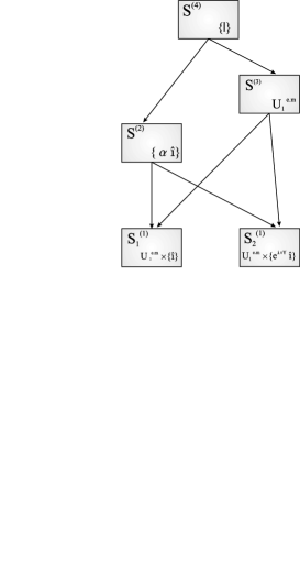
Figure 12: Stratification of the orbit space of model 1. Arrows connect higher dimensional (inner) strata to bordering lower dimensional ones. The stratum $S^{(0)}$ is not shown for simplicity. It would be connected by arrows issuing from $S^{(1)}_{1}$ and $S^{(1)}_{2}$

Making use of geometrical arguments similar to those used in the analysis of Model 0, we shall now prove that all the allowed phases of the model become observable, if the requirement of renormalizability is ignored and the dynamics of the Higgs sector is determined by a $G$-invariant polynomial potential of degree eight.

To this end, it will be sufficient to find a particular eight degree $G$-invariant polynomial $\widehat{V}_{0}^{(8)}(p)$, which, for convenient values of its coefficients, admits a stable absolute minimum in each of the strata of the orbit space of $G$. Stability is intended with respect to perturbations of $\widehat{V}_{0}^{(8)}(p)$, induced by arbitrary $G$-invariant polynomials of degree not exceeding eight.

The following simple potential is already sufficient, to make observable all the allowed phases:

$$\begin{array}[]{rcl}V^{(8)}(\phi)&=&\widehat{V}^{(8)}(p(\phi)),\\ &&\\ \widehat{V}^{(8)}(p)&=&\sum_{i=1}^{5}\,(p_{i}-\eta_{i})^{2}-\sum_{i=1}^{5}\,\eta_{i}^{2}\,,\quad p\in p({\mathbb{R}}^{8}).\end{array}$$ (47)

Stratum	Structural stability conditions
${S}^{(3)}$	$0<\lambda<2$, $\rho_{1}<0$, $-\dfrac{2\lambda\,\rho_{1}^{2}}{(2-\lambda)^{2}}<\rho_{2}<\dfrac{\rho_{1}^{2}}{4}$, $\rho_{3}>-2\lambda$,
	$-\lambda(\lambda+\rho_{3})<\rho_{4}<\dfrac{\rho_{1}^{2}}{4}$, $\lambda=\left(-\rho_{3}+\sqrt{\rho_{3}^{2}-4\rho_{4}+\alpha_{5}^{2}}\right)/2$
${S}^{(2)}$	$\rho_{1}<0$, $\rho_{2}>0$, $\rho_{3}>0$, $\alpha_{5}^{2}<\mathrm{Min}\left(2\rho_{4},4+2\rho_{3}+\rho_{4}\right)$
${S}_{1}^{(1)}$	$\alpha_{1}<0$, $\alpha_{2}>0$, $\rho_{3}>-\dfrac{8\alpha_{2}}{\alpha_{1}^{2}}$, $-\dfrac{16\alpha_{2}\left(4\alpha_{2}+\alpha_{1}^{2}\,\rho_{3}\right)}{4\alpha_{1}^{2}}<\rho_{4}<\dfrac{\rho_{3}^{2}}{4}$,
	$\alpha_{5}^{2}<4\dfrac{16\alpha_{2}^{2}+4\alpha_{1}^{2}\,\alpha_{2}\rho_{3}+\alpha_{1}^{4}\,\rho_{4}}{\alpha_{1}^{4}}$
${S}_{2}^{(1)}$	$\alpha_{1}>0,$ $\alpha_{2}<0$, $\rho_{3}>-\dfrac{8\alpha_{1}}{\alpha_{2}^{2}}$, $-\dfrac{16\alpha_{1}\left(4\alpha_{1}+\alpha_{2}^{2}\,\rho_{3}\right)}{4\alpha_{2}^{2}}<\rho_{4}<\dfrac{\rho_{3}^{2}}{4}$,
	$\alpha_{5}^{2}<4\dfrac{16\alpha_{1}^{2}+4\alpha_{2}^{2}\,\alpha_{1}\rho_{3}+\alpha_{2}^{4}\,\rho_{4}}{\alpha_{2}^{4}}$
${S}^{(0)}$	$\alpha_{1}>0,$ $\alpha_{2}>0$, $\rho_{3}>-4$, $\rho_{4}<\dfrac{\rho_{3}^{2}}{4}$, $\alpha_{5}^{2}<4+2\rho_{3}+\rho_{4}$

Table 3: Necessary and sufficient conditions for structural stability of the allowed phases in Model $1_{1}$, for $A=1\!\!1$. The phase corresponding to the principal stratum is dynamically unattainable. In the table, the results are expressed also in terms of the following functions of the control parameters: $\rho_{1}=\alpha_{1}+\alpha_{2}$, $\rho_{2}=\alpha_{1}\,\alpha_{2}$, $\rho_{3}=\alpha_{3}+\alpha_{4}$, $\rho_{4}=\alpha_{3}\,\alpha_{4}$.

In fact, it is easy to realize that, for each given choice of $\eta$, thought of as a point in the $p$-space, the absolute minimum of the potential $\widehat{V}^{(8)}(p)$ is located at the points $\bar{p}$ of the orbit space which is nearest to $\eta$. The minimum at the point $\bar{p}$, sitting on the stratum $\bar{S}$, is non degenerate, if $\eta$ is close enough to $\bar{S}$ in the intersection of the normal spaces at $\bar{p}$ to the higher dimensional strata bordering $\bar{S}$. The geometrical feature of the orbit space, that guarantees the existence and uniqueness of a point of the orbit space at minimum distance from $\eta$, under the conditions just specified, is the absence of intruding cusps (see Figure 11).

The above statements have been checked analytically. Constraints on the values of the control parameters $\eta_{i}$ which are sufficient to guarantee the location and stability of the absolute minimum in the different strata are listed in Table 4.

Stratum	Structural stability conditions
$S^{(4)}$	$\mu_{1}>0,\;\;\mu_{2}>0,\;\;0<\mu_{3}<\mu_{2}$, $\dfrac{2}{9}{\mu_{3}}^{2}<\mu_{4}<\dfrac{{\mu_{3}}^{2}}{4}$, $0<{\eta_{5}}^{2}<\mu_{4}$
$S^{(3)}$	$\mu_{1}>0\,,\;\;\mu_{2}>0\,,\;\;0<\mu_{3}<\dfrac{3}{2}\mu_{2}$, $-\mu_{2}\,(\mu_{2}-\mu_{3})<\mu_{4}<\dfrac{{\mu_{3}}^{2}}{4}$
$S^{(2)}$	$\eta_{1}>0\,,\;\;\eta_{2}>0\,,\;\;\eta_{3}<0\,,\,\;\eta_{4}<0$
${S}_{1}^{(1)}$	$\eta_{1}>0\,,\;\eta_{2}<0$, $\eta_{3}+\eta_{4}<-\dfrac{2\eta_{2}}{\eta_{1}}$, $\eta_{3}\,\eta_{4}<-\dfrac{4\eta_{2}\left[\eta_{2}+\eta_{1}(\eta_{3}+\eta_{4})\right]}{3{\eta_{1}}^{2}}$
${S}_{1}^{(2)}$	$\eta_{1}<0$, $\eta_{2}>0$, $\eta_{3}+\eta_{4}<-\dfrac{2\eta_{1}}{{\eta_{2}}^{2}}$, $\eta_{3}\,\eta_{4}<-\dfrac{4\eta_{1}\left[\eta_{1}+{\eta_{2}}^{2}(\eta_{3}+\eta_{4})\right]}{3{\eta_{2}}^{4}}$
$S^{(0)}$	$\eta_{1}\,,\;\eta_{2}<0$

Table 4: Sufficient conditions for structural stability of the phases $\mathcal{F}^{(i)}_{j}$ associated to strata $S^{(i)}_{j}$ of Model $1_{2}$. In the table, the results are expressed also in terms of the following functions of the control parameters: $\mu_{1}=\eta_{1}+\eta_{2}$, $\mu_{2}=\eta_{1}\,\eta_{2}$, $\mu_{3}=\eta_{3}+\eta_{4}$ and $\mu_{4}=\eta_{3}\,\eta_{4}$.

4.3 Model 2: Implementing a CP–like discrete symmetry in Model 1

In the model studied in [12, 13] the role of the discrete symmetry is fundamental in achieving the possibility of a two stage phase transition. The main advantage advocated by the authors is an amplification of the CP-violating effects. Since the experimental information on the Higgs sector are at present very weak and not enough to fully determine the discrete symmetries in two-Higgs-doublet models, the addition of some discrete symmetry could allow some subtler amplification pattern. Moreover, from a technical point of way, adding some discrete symmetry allows to construct symmetry group representations with a lower level of non-coregularity, which implies easier computations in the framework of the orbit space approach. Therefore in this subsection we shall consider a model with the same set of fields as Model 1, but with symmetry group SU${}_{2}\times\mathrm{U}_{1}\times\{\hat{\iota}\,,K\}$, where $\hat{\iota}$ is the generator of a reflection group and $K$ is the generator of a $CP$-like transformation: $(\Phi_{1},\Phi_{2})\rightarrow(\Phi_{1},-\Phi_{2})$ and $(\Phi_{1},\Phi_{2})\rightarrow(\Phi_{1}^{*},\Phi_{2}^{*})$, respectively. The addition of a new discrete symmetry will increase the number of allowed phases.

Stratum	Symmetry	Typical point $\phi$
${S}^{(4)}$	$\{1\!\!1\}$	$(\phi_{1},0,\phi_{3},\phi_{4},0,0,\phi_{7},0)$
${S}^{(3)}_{1}$	$\{\hat{\iota}\,K\}$	$(\phi_{1},0,\phi_{3},0,0,0,0,\phi_{8})$
${S}^{(3)}_{2}$	$\{K\}$	$(\phi_{1},0,\phi_{3},0,0,0,\phi_{7},0)$
${S}^{(3)}_{3}$	U${}_{1}^{\mathrm{e}.m.}$	$(0,0,\phi_{3},\phi_{4},0,0,\phi_{7},0)$
${S}^{(2)}_{1}$	$\{\alpha\,\hat{\iota},K\}$	$(\phi_{1},0,0,0,0,0,\phi_{7},0)$
${S}^{(2)}_{2}$	U${}_{1}^{\mathrm{e}.m.}\times\,\{\hat{\iota}\,K\}$	$(0,0,\phi_{3},0,0,0,0,\phi_{8})$
${S}^{(2)}_{3}$	U${}_{1}^{\mathrm{e}.m.}\times\{K\}$	$(0,0,\phi_{3},0,0,0,\phi_{7},0)$
${S}^{(1)}_{1}$	U${}_{1}^{\mathrm{e}.m.}\,\times\{\hat{\iota},K\}$	$(0,0,\phi_{3},0,0,0,0,0)$
${S}^{(1)}_{2}$	U${}_{1}^{\mathrm{e}.m.}\times\{e^{i\pi Y}\,\hat{\iota},K\}$	$(0,0,0,0,0,0,\phi_{7},0)$
${S}^{(0)}$	$(\mathrm{SU}_{2}\times\mathrm{U}_{1})/{\mathbb{Z}}_{2}\,\times\{\hat{\iota}\,,\;K\}$	$(0,0,0,0,0,0,0,0)$

Table 5: Symmetries of the strata ${S}$ of Model 2. The group $\mathrm{U}_{1}^{\mathrm{e.m.}}$ is defined as in Table 1, and $\alpha=\mathrm{e}^{\mathrm{i}\pi(T_{3}-Y/2)}$. Symmetries are specified by a representative element of the conjugacy class of isotropy subgroups. Finite groups are defined through their generators between brackets. For each stratum, a field configuration with the same symmetry is supplied (typical point). The $\phi_{i}$’s are generic non zero values.

Stratum	Defining relations	Symmetry	Boundary
${S}^{(4)}$	${p}_{1},{p}_{3},{p}_{4},{p}_{1}{p}_{2}-{p}_{3}-{p}_{4}>0$	$\{1\!\!1\}$	$\overline{{S}_{i}^{(3)}},i=1,2,3$
${S}^{(3)}_{1}$	${p}_{3}=0<{p}_{4}<{p}_{1}{p}_{2}\,,\;p_{1}+p_{2}>0$	$\{\hat{\iota}\,K\}$	$\overline{{S}_{i}^{(2)}},i=1,2$
${S}^{(3)}_{2}$	${p}_{4}=0<{p}_{3}<{p}_{1}{p}_{2}\,,\;p_{1}+p_{2}>0$	$\{K\}$	$\overline{{S}_{i}^{(2)}},i=1,3$
${S}^{(3)}_{3}$	${p}_{1}{p}_{2}-{p}_{3}-{p}_{4}=0<{p}_{1}+p_{2},\,{p}_{3},\,{p}_{4}$	U${}_{1}^{\rm e.m.}$	$\overline{{S}_{i}^{(2)}},i=2,3$
${S}^{(2)}_{1}$	${p}_{3}={p}_{4}=0<{p}_{1},\,{p}_{2}$	$\{\alpha\,\hat{\iota},K\}$	$\overline{{S}_{i}^{(1)}},i=1,2$
${S}^{(2)}_{2}$	${p}_{1}{p}_{2}-{p}_{4}={p}_{3}=0<{p}_{1}+{p}_{2},\,p_{4}$	U${}_{1}^{\rm e.m.}\times\{\hat{\iota}\,K\}$	$\overline{{S}_{i}^{(1)}},i=1,2$
${S}^{(2)}_{3}$	${p}_{1}{p}_{2}-{p}_{3}={p}_{4}=0<{p}_{1}+{p}_{2},\,p_{3}$	U${}_{1}^{\rm e.m.}\times\{K\}$	$\overline{{S}_{i}^{(1)}},i=1,2$
${S}^{(1)}_{1}$	${p}_{2}={p}_{3}={p}_{4}=0<{p}_{1}$	U${}_{1}^{\rm e.m.}\times\{\hat{\iota},K\}$	${S}^{(0)}$
${S}^{(1)}_{2}$	${p}_{1}={p}_{3}={p}_{4}=0<{p}_{2}$	U${}_{1}^{\rm e.m.}\times\{{\rm e}^{i\pi Y}\hat{\iota},K\}$	${S}^{(0)}$
${S}^{(0)}$	${p}_{1}={p}_{2}={p}_{3}={p}_{4}=0$	(SU${}_{2}\times$U${}_{1})/{\mathbb{Z}}_{2}\,\times\{\hat{\iota},K\}$

Table 6: Symmetries and defining relations of the strata $S$ of Model 2. The symmetries are specified by means of a “representative” element of the conjugacy class of isotropy subgroups. Finite groups are specified through their generators written between brackets and $\alpha=e^{i\pi(T_{3}-Y/2)}$. Continuous phase transitions are possible only between bordering strata. The group U${}_{1}^{\rm e.m.}$ is the subgroup of SU${}_{2}\times$U₁ formed by the elements $({\rm diag}\{e^{i\theta},e^{-i\theta}\},e^{i\theta})$ and U${}_{1}^{\rm e.m.}(\pi)$ denotes its element $({\rm diag}\{-1,1\},-1)$.

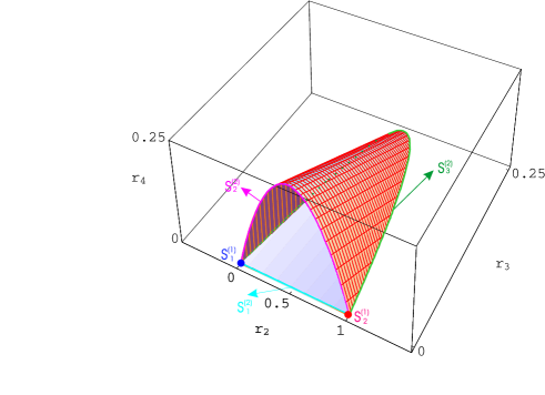
Figure 13: Section $\Xi$ of the four dimensional orbit space of Model 2 with the hyperplane of equation $p_{1}+p_{2}=1$. The one dimensional strata are represented by the blue and red points. The pale blue, pink and green lines represent the two dimensional strata $S^{(2)}_{1}$, $S^{(2)}_{2}$ and $S^{(2)}_{3}$, respectively. $\Xi$ looks like a cave, whose entrance, floor, ceiling and interior are formed by the strata $S^{(3)}_{1}$, $S^{(3)}_{2}$, $S^{(3)}_{3}$ and $S^{(4)}$, respectively. The relations defining the strata can be found in Table 6.

As in model 1, for our purposes it will be equivalent, but simpler, to consider as a symmetry group of the model $G=$ (SU${}_{2}\times\mathrm{U}_{1})/{\mathbb{Z}}_{2}\,\times\{\hat{\iota}\,,\,K\}$. Under these assumptions, a MIB is the following:

$$\begin{array}[]{l}{p}_{1}=\Phi_{1}^{\dagger}\Phi_{1},\;\;{p}_{2}=\Phi_{2}^{\dagger}\Phi_{2},\\ \\ {p}_{3}=\left(\mathrm{Re}\left[\Phi_{2}^{\dagger}\Phi_{1}\right]\right)^{2},\;\;{p}_{4}=\left(\mathrm{Im}\left[\Phi_{2}^{\dagger}\Phi_{1}\right]\right)^{2}.\end{array}$$ (48)

The defining relations of the strata of ${p}({\mathbb{R}}^{8})$ can be obtained from positivity and rank conditions of the symmetric matrix $\widehat{P}({p})$, associated to the MIB defined in (48):

$${\widehat{P}(p)=4\left(\begin{array}[]{cccc}{p}_{1}&0&{p}_{3}&{p}_{4}\\ 0&{p}_{2}&{p}_{3}&{p}_{4}\\ {p}_{3}&{p}_{3}&\,p_{3}({p}_{1}+{p}_{2})&0\\ {p}_{4}&{p}_{4}&0&{p}_{4}\,({p}_{1}+{p}_{2})\end{array}\right).}$$ (49)

The results are shown in Tables 5 and 6.

The section $\Xi$ of ${p}({\mathbb{R}}^{8})\subset{\mathbb{R}}^{4}$ with the hyperplane of equation ${p}_{1}+{p}_{2}=1$ is the three dimensional closed solid (semialgebraic set) shown in Figure 13. The full orbit space is the four dimensional connected semi-algebraic set formed by the points ${p}=({p}_{1},{p}_{2},{p}_{3},{p}_{4})=\Pi^{-1}(r)$, $r\in\Xi$, where $\Pi^{-1}$ is the inverse projection defined as follows:

$$\begin{array}[]{lccl}\Pi^{-1}:&{\mathbb{R}}^{3}\supset\Xi&\longrightarrow&{\mathbb{R}}^{4}\\ &(r_{2},r_{3},r_{4})&\mapsto&\left(\lambda(1-r_{2}),\lambda r_{2},\lambda^{2}r_{3},\lambda^{2}r_{4}\right)\,,\hskip 20.00003pt\lambda\geq 0\,.\end{array}$$ (50)

For the ease of the reader a scheme of the stratification of the model is shown in Fig. 14.

We shall consider two different dynamical versions of Model 2, a complete non-renormalizable and an incomplete renormalizable one.

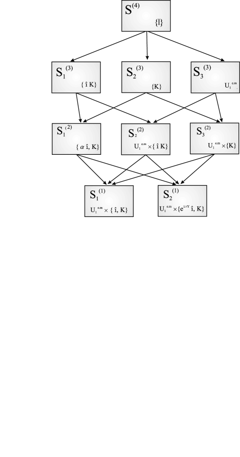
Figure 14: Stratification of the orbit space of model 2. Arrows connect higher dimensional (inner) strata to bordering lower dimensional ones. The stratum $S^{(0)}$ is not shown for simplicity. It would be connected by arrows issuing from $S^{(1)}_{1}$ and $S^{(1)}_{2}$

The $CP$-like transformation we have defined allows an easy verification of $CP$ conservation. For example, with reference to Tables 5 and 6, it is evident that $CP$ is broken in the stratum ${S}^{(3)}_{3}$, while $CP$ is conserved in ${S}^{(2)}_{2}$: the transformations induced by $\hat{\iota}$ determine the right $CP$-phase $\theta$ for each field of the theory.

4.3.1 Model $2_{1}$: An incomplete renormalizable version of Model 2

Let us now, in the frame of symmetries of Model 2, chose the Higgs potential as the most general, bounded below invariant polynomial of degree four:

$$\widehat{V}^{(4)}({p})=\sum_{i,j=1}^{2}\,A_{ij}\,{p}_{i}\,{p}_{j}+\sum_{i=1}^{4}\,\alpha_{i}\,{p}_{i},$$ (51)

where all the parameters are real, $A_{12}=A_{21}$ and the inequalities in the first line of Eq. (45) make sure that $V^{(4)}(p(\phi))$ diverges to $+\infty$ for $\|\phi\|\to\infty$.

As stated in [5, 23], since there are no relations among the elements of the MIB and the potential is linear in the basic invariants of degree four, its local minima can only sit on the boundary of the orbit space, for general values of the $\alpha_{i}$’s. The result of a detailed calculation is shown in Table 7: we have listed the values of the $\alpha_{i}$’s that guarantee the location of a stable absolute minimum of $\widehat{V}(p)$ in the different strata, for $A=1\!\!1$. In fact, there can be stationary points of the potential in the strata of dimension $\geq 3$ only if the $\alpha_{i}$’s satisfy particular conditions: $\alpha_{3}=\alpha_{4}=0$, $\alpha_{4}=0$, $\alpha_{3}=0$ and $\alpha_{3}=\alpha_{4}$, respectively, for the strata ${S}^{(4)}$, ${S}^{(3)}_{1}$, ${S}^{(3)}_{2}$ and ${S}^{(3)}_{3}$.

Stratum	Structural stability conditions
${S}^{(2)}_{1}$	$\alpha_{1}<0,$ $\alpha_{2}<0,$ $\alpha_{3}>0,$ $\alpha_{4}>0$
${S}^{(2)}_{2}$	$-2<\alpha_{4}<0,$ $\alpha_{3}>\alpha_{4},$ $\left(\alpha_{1}<0,\;\;\alpha_{2}<\dfrac{\alpha_{1}\alpha_{4}}{2}\right)$ or
	$\left(\alpha_{1}>0,\;\;\alpha_{2}>\dfrac{2\alpha_{1}}{\alpha_{4}}\right)$
${S}^{(2)}_{3}$	$-2<\alpha_{3}<0,$ $\alpha_{4}>\alpha_{3},$ $\left(\alpha_{1}<0,\;\;\alpha_{2}<\dfrac{\alpha_{1}\alpha_{3}}{2}\right)$ or
	$\left(\alpha_{1}>0,\;\;\alpha_{2}>\dfrac{2\alpha_{1}}{\alpha_{3}}\right)$
${S}_{1}^{(1)}$	$\alpha_{1}<0,$ $\alpha_{2}>0,$ $\alpha_{3}>\mathrm{Max}\left(2\dfrac{\alpha_{2}}{\alpha_{1}},-2\right)$, $\alpha_{4}>\mathrm{Max}\left(2\dfrac{\alpha_{2}}{\alpha_{1}},-2\right)$
${S}_{1}^{(2)}$	$\alpha_{1}>0,$ $\alpha_{2}<0,$ $\alpha_{3}>\mathrm{Max}\left(2\dfrac{\alpha_{1}}{\alpha_{2}},-2\right)$, $\alpha_{4}>\mathrm{Max}\left(2\dfrac{\alpha_{1}}{\alpha_{2}},-2\right)$
${S}^{(0)}$	$\alpha_{1}>0,$ $\alpha_{2}>0,$ $\alpha_{3}>-2,$ $\alpha_{4}>-2$

Table 7: Necessary and sufficient conditions for structural stability of the phases ${\mathcal{F}}^{(i)}_{j}$ associated to the strata ${\mathcal{S}}^{(i)}_{j}$ of 2₁, for $A=1\!\!1$. The strata not appearing in the table are physically unattainable.

These conditions reduce to zero the measures of the regions of stability of the corresponding phases, in the space of the parameters $\alpha_{i}$. So, there will not be stable phases associated to the strata of dimension $\geq 3$. As a consequence, it is impossible to generate spontaneous $CP$ violation in the model. The general problem of spontaneous $CP$ breaking in two-Higgs doublet models will be faced in a forthcoming paper [31].

We can conclude that Model $2_{1}$ is renormalizable, but it is incomplete.

4.3.2 Model $2_{2}$: A complete non-renormalizable version of Model 2

Stratum	Structural stability conditions
$S^{(4)}$	$\eta_{1}>0\,,\;\;\eta_{2}>0\,,\;\;0<\eta_{3}<\eta_{1}\eta_{2}\,,\;\;0<\eta_{4}<\eta_{1}\eta_{2}-\eta_{3}$
$S^{(3)}_{1}$	$\eta_{1}>0\,,\;\;\eta_{2}>0\,,\;\;\eta_{3}<0\,,\;\;0<\eta_{4}<\eta_{1}\eta_{2}$
${S}^{(3)}_{2}$	$\eta_{1}>0\,,\;\;\eta_{2}>0\,,\;\;0<\eta_{3}<\eta_{1}\eta_{2}\,,\;\;\eta_{4}<0$
${S}^{(3)}_{3}$	$0<\lambda<2\,,\;\;\mu_{1}>0\,,\;\;-\dfrac{2\lambda}{(\lambda-2)^{2}}\mu_{1}^{2}<\mu_{2}<\dfrac{\mu_{1}^{2}}{4}$
	$\dfrac{\lambda}{2}<\eta_{4}<\left(\dfrac{1}{2}+\dfrac{8\mu_{1}^{2}}{(\lambda^{2}-4)^{2}}\right)\lambda+\dfrac{4\mu_{2}}{(\lambda+2)^{2}}$
	$\eta_{3}=-\eta_{4}+\dfrac{\lambda\left((\lambda^{2}-4)^{2}+8\mu_{1}^{2}\right)+4\mu_{2}(\lambda-2)^{2}}{(\lambda^{2}-4)^{2}}$
${S}^{(2)}_{1}$	$\eta_{1}>0\,,\;\;\eta_{2}>0\,,\;\;\eta_{3}<0\,,\;\;\eta_{4}<0$
${S}^{(2)}_{2}$	$0<\lambda<2\,,\;\;\mu_{1}>0\,,\;\;-\dfrac{2\lambda}{(\lambda-2)^{2}}\mu_{1}^{2}<\mu_{2}<\dfrac{\mu_{1}^{2}}{4}\,,\;\;\eta_{3}<\dfrac{\lambda}{2}$
	$\eta_{4}=\dfrac{\lambda\left((\lambda^{2}-4)^{2}+16\mu_{1}^{2}\right)+8\mu_{2}(\lambda-2)^{2}}{2(\lambda^{2}-4)^{2}}$
${S}^{(2)}_{3}$	$0<\lambda<2\,,\;\;\mu_{1}>0\,,\;\;-\dfrac{2\lambda}{(\lambda-2)^{2}}\mu_{1}^{2}<\mu_{2}<\dfrac{\mu_{1}^{2}}{4}\,,\;\;\eta_{4}<\dfrac{\lambda}{2}$
	$\eta_{3}=\dfrac{\lambda\left((\lambda^{2}-4)^{2}+16\mu_{1}^{2}\right)+8\mu_{2}(\lambda-2)^{2}}{2(\lambda^{2}-4)^{2}}$
${S}_{1}^{(1)}$	$\eta_{1}>0\,,\;\;\eta_{2}<0\,,\;\;\eta_{3}<-\dfrac{\eta_{2}}{\eta_{1}}\,,\;\;\eta_{4}<-\dfrac{\eta_{2}}{\eta_{1}}$
${S}_{1}^{(2)}$	$\eta_{1}<0\,,\;\;\eta_{2}>0\,,\;\;\eta_{3}<-\dfrac{\eta_{1}}{\eta_{2}}\,,\;\;\eta_{4}<-\dfrac{\eta_{1}}{\eta_{2}}$
${S}^{(0)}$	$\eta_{1}<0\,,\;\;\eta_{2}<0$

Table 8: Sufficient conditions for structural stability of the phases ${\mathcal{F}}^{(i)}_{j}$ associated to the strata ${\mathcal{S}}^{(i)}_{j}$ of 2₂. In the table the results are expressed also in terms of the following functions of the control parameters: $\mu_{1}=\eta_{1}+\eta_{2}$ and $\mu_{2}=\eta_{1}\,\eta_{2}$.

If renormalizability conditions are dropped, the simple potential defined in (40), with the ${p}_{i}$’s specified in (48), is already sufficient to make observable all the allowed phases. It admits, in fact, a stable minimum in each of the strata listed in Tables 5 and 6, for suitable values of the $\eta_{i}$’s, as can be easily realized, with the help of Figure 13, by conveniently modifying the geometrical arguments exploited to determine the observable phases of Model 1. The transformation in Eq. (50) leads to a four dimensional semialgebraic set which, contrary to $\Xi$, is not convex, but, fortunately, like $\Xi$, has no intruding cusps. In particular, for $A\propto 1\!\!1$ let us think of $\eta$ as a point in the $p$-space. Then, if $\eta$ is within or near enough to the orbit space, there is only one local minimum of the potential (the absolute minimum) at the point ${p}$ of the orbit space which is nearest to $\eta$.

The above statements have been checked analytically: sufficient conditions for structural stability are expressed in Table 8, page 8.

5 Complete renormalizable two-Higgs-doublet $+$ singlet extensions of the SM

In the previous sections we have shown that it is possible to obtain complete models provided that renormalizability is given up in the Higgs potential. This could be rightly assessed to be too high a sacrifice.

In this section we shall propose a cheaper achievement of completeness in the incomplete 2HD models studied in Section 4. It is obtained by extending the models by adding one or two scalar singlets with convenient transformation properties under the discrete symmetries. The addition of scalar fields obviously modifies the linear symmetry group $G$ of the Higgs sector, i.e. the symmetry of the model, and extends the set of allowed phases. The important point is that both the allowed phases of the original models and the newly originated ones turn out to be observable in the extended versions of the models. Whether or not the increase in the number of phases is welcome can only be decided on the basis of an analysis of the phenomenological consequences of the models.

5.1 Model 1C: A complete renormalizable extension of Model 1

In this subsection, we shall show that the addition to Model 1 of a real SU${}_{2}\times\mathrm{U}_{1}$-singlet, $\phi_{9}$, with transformation rule $\hat{\iota}\,:\;\phi_{9}\rightarrow-\phi_{9}$ under the reflection $\hat{\iota}$, is sufficient to make observable all the phases allowed by the symmetry of the extended model, that we shall call Model 1C.

A MIB for the linear group $G=\left((\mathrm{SU}_{2}\times\mathrm{U}(1))/{\mathbb{Z}}_{2}\times\{\widehat{i}\},\ {\underline{9}}\right)$, acting on the nine independent scalar fields of the model, is made up of the following eight invariants:

$${\begin{array}[]{lcl}p_{1}=\Phi_{1}^{\dagger}\Phi_{1},\;\;\;p_{2}=\Phi_{2}^{\dagger}\Phi_{2},&&p_{3}=\phi_{9}^{2},\;\;\;p_{4}=\mathrm{Re}\left[\Phi_{2}^{\dagger}\Phi_{1}\right]\phi_{9},\\ &&\\ p_{5}=\mathrm{Im}\left[\Phi_{2}^{\dagger}\Phi_{1}\right]\,\phi_{9},&&p_{6}=\mathrm{Re}\left[\Phi_{2}^{\dagger}\Phi_{1}\right]^{2},\\ &&\\ p_{7}=\mathrm{Im}\left[\Phi_{2}^{\dagger}\Phi_{1}\right]^{2},&&p_{8}=\mathrm{Re}\left[\Phi_{2}^{\dagger}\Phi_{1}\right]\,\mathrm{Im}\left[\Phi_{2}^{\dagger}\Phi_{1}\right]\;.\end{array}}$$ (52)

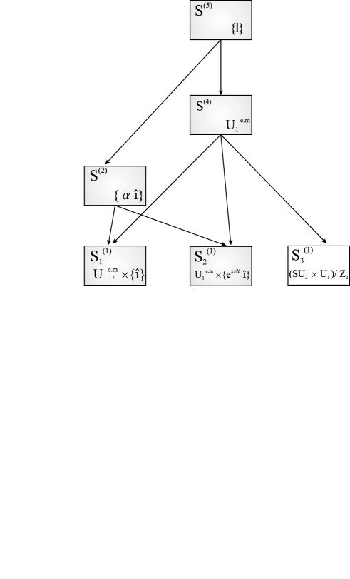
Figure 15: Stratification of model 1C. A unique new phase ${\mathcal{F}}_{3}^{(1)}$ associated to the stratum $S_{3}^{(1)}$ is added to the set of allowed phases of Model 1 (grey boxes). The stratum $S^{(0)}$ is not shown for simplicity. It would be connected by arrows issuing from $S^{(1)}_{1}$, $S^{(1)}_{2}$ and $S^{(1)}_{3}$.

The elements of the MIB have degrees $\{2,2,2,3,3,4,4,4\}$ and are related by six syzygies $s_{i}=0$:

$${\begin{array}[]{rcl}s_{1}&=&p_{4}^{2}-p_{3}\,p_{6},\ s_{2}=p_{5}^{2}-p_{3}\,p_{7},\ s_{3}=p_{8}^{2}-p_{6}\,p_{7},\\ s_{4}&=&p_{4}\,p_{8}-p_{5}\,p_{6},\ s_{5}=p_{3}\,p_{8}-p_{4}\,p_{5},\ s_{6}=p_{5}\,p_{8}-p_{4}\,p_{7}.\end{array}}$$ (53)

Only three of the syzygies are independent. Therefore, the orbit space is a semialgebraic subset of the five dimensional algebraic variety of the $p$-space ${\mathbb{R}}^{8}$, defined by the set of equations $s_{i}=0$, $i=1,\dots,6$. As usual, the relations defining the orbit space and its stratification can be determined from rank and positivity conditions of the $\widehat{P}(p)$-matrix associated to the MIB defined in (52). The results are reported in Tables 9 and 10.

The only non-vanishing upper triangular elements of the $\widehat{P}$-matrix turn out to be the following:

$$\widehat{P}_{i\,i} = 4p_{i}\;\;\mbox{\rm for}\;\;i=1,2,3\,,$$

$$\widehat{P}_{4\,4} = (p_{1}+p_{2})p_{3}+p_{6}\,,$$

$$\widehat{P}_{5\,5} = (p_{1}+p_{2})p_{3}+p_{7}\,,$$

$$\widehat{P}_{j\,j} = 4\left(p_{1}+p_{2}\right)\,p_{j}\;\;\mbox{\rm for}\;\;j=6,7\,,$$

$$\widehat{P}_{8\,8} = (p_{1}+p_{2})(p_{6}+p_{7})\,,$$

$$\widehat{P}_{i\,j} = 2p_{j}\;\;\mbox{\rm for}\;\;i=1,2,3\,\;\mbox{\rm and}\,j=4,5\,,$$

$$\widehat{P}_{i\,j} = 4p_{j}\;\;\mbox{\rm for}\;\;i=1,2\,\;\mbox{\rm and}\,j=6,7\,,$$

$$\widehat{P}_{i\,8} = 4p_{8}\;\;\mbox{\rm for}\;\;i=1,2\,,$$

$$\widehat{P}_{4\,5} = p_{8}\,,$$

$$\widehat{P}_{4\,6} = 2\widehat{P}_{5\,8}=2(p_{1}+p_{2})p_{4}\,,$$

$$\widehat{P}_{5\,7} = 2\widehat{P}_{4\,8}=2(p_{1}+p_{2})p_{5}\,,$$

$$\widehat{P}_{i\,8} = 2(p_{1}+p_{2})p_{8}\,,\mbox{\rm for}\;\;i=6,7\,.$$

Stratum	Symmetry	Typical point $\phi$
$S^{(5)}$	$\{1\!\!1\}$	$(\phi_{1},0,\phi_{3},\phi_{4},0,0,\phi_{7},0,\phi_{9})$
$S^{(4)}$	U${}_{1}^{\mbox{\rm e.m.}}$	$(0,0,\phi_{3},\phi_{4},0,0,\phi_{7},0,\phi_{9})$
$S^{(2)}$	$\{\alpha\hat{i}\}$	$(\phi_{1},0,0,0,0,0,\phi_{7},0,0)$
$S^{(1)}_{1}$	U${}_{1}^{\mbox{\rm e.m.}}\times\{\hat{i}\}$	$(0,0,\phi_{3},0,0,0,0,0,0)$
$S^{(1)}_{2}$	U${}_{1}^{\mbox{\rm e.m.}}\times\{e^{i\pi Y}\,\hat{i}\}$	$(0,0,0,0,0,0,\phi_{7},0,0)$
$S^{(1)}_{3}$	$(\mathrm{SU}_{2}\times\mathrm{U}_{1})/{\mathbb{Z}}_{2}$	$(0,0,0,0,0,0,0,0,\phi_{9})$
$S^{(0)}$	$(\mathrm{SU}_{2}\times\mathrm{U}_{1})/{\mathbb{Z}}_{2}\,\times\{\hat{\iota}\}$	$(0,0,0,0,0,0,0,0,0)$

Table 9: Symmetries of the strata of Model 1C. The group $\mathrm{U}_{1}^{\mathrm{e.m.}}$ is defined as in Table 1, and $\alpha=\mathrm{e}^{\mathrm{i}\pi(T_{3}-Y/2)}$. Symmetries are specified by a representative element of the conjugacy class of isotropy subgroups. Finite groups are defined through their generators between brackets. For each stratum, a field configuration with the same symmetry is supplied (typical point). The $\phi_{i}$’s are generic non zero values.

Stratum	Defining relations	Boundary
$S^{(5)}$	$s_{i}=0\,,1\leq i\leq 6$	$\overline{S^{(4)}}\,,\overline{S^{(2)}}$
	$p_{1}p_{2}-p_{6}-p_{7}>0\,,\;p_{1}+p_{2}>0$
	$p_{j}\geq 0\,,\;\;j=1,2,3,6,7.$
$S^{(4)}$	$s_{i}=0\,,1\leq i\leq 6$	$\overline{S^{(1)}_{j}}\,,\;1\leq j\leq 3$
	$p_{6}+p_{7}-p_{1}p_{2}=0\,,$
	$p_{i}+p_{j}>0\,,\;(i,j)=(1,2)\;\mbox{\rm{and}}\;(1,3)\;\mbox{\rm{and}}\;(2,3)$
	$p_{k}\geq 0\,,\;1\leq k\leq 3$
$S^{(2)}$	$p_{j}=0<p_{1}\,,p_{2}\,,\;\;\;j\neq 1,2$	$\overline{S^{(1)}_{j}}\,,\;1\leq j\leq 2$
$S^{(1)}_{1}$	$p_{i}=0<p_{1}\,,\;\;\;i\neq 1$	$S^{(0)}$
$S^{(1)}_{2}$	$p_{i}=0<p_{2}\,,\;\;\;i\neq 2$	$S^{(0)}$
$S^{(1)}_{3}$	$p_{i}=0<p_{3}\,,\;\;\;i\neq 3$	$S^{(0)}$
$S^{(0)}$	$p_{i}=0,\quad 1\leq i\leq 8$

Table 10: Stratification of the orbit space of Model 1C. The syzygies are $s_{1}=p_{4}^{2}-p_{3}p_{6}$, $s_{2}=p_{5}^{2}-p_{3}p_{7}$, $s_{3}=p_{8}^{2}-p_{6}p_{7}$, $s_{4}=p_{4}p_{8}-p_{5}p_{6}$, $s_{5}=p_{3}p_{8}-p_{4}p_{5}$, $s_{6}=p_{5}p_{8}-p_{4}p_{7}$. Neighboring strata are indicated, so that possible second order phase transitions can be easily identified.

As expected, a new phase, $S^{(1)}_{3}$, is now allowed.

The most general invariant polynomial of degree four in the scalar fields of the model can be written in the following form:

$${\widehat{V}^{(4)}(p)=\sum_{i=1}^{8}\,\alpha_{i}\,p_{i}+\sum_{i,j=1}^{3}\,A_{ij}\,p_{i}\,p_{j}\,,}$$ (54)

where, to guarantee that the potential is bounded from below, we assume that all the coefficients are real, the symmetric matrix $A$ is positive definite and

$$A_{11},A_{22}>0,\quad\alpha_{6},\alpha_{7}>-2\left(A_{12}+\sqrt{A_{11}\,A_{22}}\right),$$

(55)

$$\alpha_{8}^{2}<4\left[\alpha_{6}+2\left(A_{12}+\sqrt{A_{11}\,A_{22}}\right)\right]\times\left[\alpha_{7}+2\left(A_{12}+\sqrt{A_{11}\,A_{22}}\right)\right]\,.$$

The conditions for the occurrence of a stationary point of $\widehat{V}^{(4)}(p)$ in a given stratum are obtained from equation (36) and the explicit form of the relations defining the strata can be read from Table 10.

Stratum	Structural stability conditions
$S^{(5)}$	$\alpha_{2}<0\,,\;\alpha_{6}>0\,,\;\alpha_{7}>0\,,\;4\alpha_{6}\alpha_{7}-\alpha_{8}^{2}>0\,,\;\alpha_{3}<\dfrac{\alpha_{5}^{2}\alpha_{6}+\alpha_{4}^{2}\alpha_{7}-\alpha_{4}\alpha_{5}\alpha_{8}}{4\alpha_{6}\alpha_{7}-\alpha_{8}^{2}}\,,\;$
	$\alpha_{8}\left(-2\alpha_{5}\alpha_{6}+\alpha_{4}\alpha_{8}\right)\left(-2\alpha_{4}\alpha_{7}+\alpha_{5}\alpha_{8}\right)>0\,,\;$
	$\alpha_{1}<\dfrac{2\left[{{{\alpha}_{5}}}^{2}\,{{\alpha}_{6}}+{{{\alpha}_{4}}}^{2}\,{{\alpha}_{7}}-{{\alpha}_{4}}\,{{\alpha}_{5}}\,{{\alpha}_{8}}+{{\alpha}_{3}}\,\left(-4\,{{\alpha}_{6}}\,{{\alpha}_{7}}+{{{\alpha}_{8}}}^{2}\right)\right]}{\left(4\,\alpha_{6}\,\alpha_{7}-\alpha_{8}^{2}\right)^{3}\,}\times$
	$\hskip 25.0pt\times\dfrac{\left[-4\,{{\alpha}_{4}}\,{{\alpha}_{5}}\,\left({{\alpha}_{6}}+{{\alpha}_{7}}\right)\,{{\alpha}_{8}}+{{{\alpha}_{5}}}^{2}\,\left(4\,{{{\alpha}_{6}}}^{2}+{{{\alpha}_{8}}}^{2}\right)+{{{\alpha}_{4}}}^{2}\,\left(4\,{{{\alpha}_{7}}}^{2}+{{{\alpha}_{8}}}^{2}\right)\right]}{\alpha_{2}\,\alpha_{9}}<0$
$S^{(4)}$	$0<\lambda<2\,,\;\alpha_{6}>-\lambda\,,\;\alpha_{7}>-\lambda\,,\;\rho_{1}<0\,,\;-\dfrac{2\lambda}{(\lambda-2)^{2}}\rho_{1}^{2}<\rho_{2}<\dfrac{1}{4}\rho_{1}^{2}\,,\;$
	$\alpha_{8}^{2}<4\left(\alpha_{6}+\lambda\right)\left(\alpha_{7}+\lambda\right)\,,\;\alpha_{8}\left[\alpha_{4}\alpha_{8}-2\alpha_{5}\left(\alpha_{6}+\lambda\right)\right]\left[\alpha_{5}\alpha_{8}-2\alpha_{4}\left(\alpha_{7}+\lambda\right)\right]>0\,,\;$
	$\!\!\!\!\!\!\!\!\rho_{1}<\dfrac{\left(-2+\lambda\right)\,{\left(-4\,{{\alpha}_{4}}\,{{\alpha}_{5}}\,\left(2\,\lambda+{{\alpha}_{6}}+{{\alpha}_{7}}\right)\,{{\alpha}_{8}}+{{{\alpha}_{5}}}^{2}\,\left(4\,{\left(\lambda+{{\alpha}_{6}}\right)}^{2}+{{{\alpha}_{8}}}^{2}\right)+{{{\alpha}_{4}}}^{2}\,\left(4\,{\left(\lambda+{{\alpha}_{7}}\right)}^{2}+{{{\alpha}_{8}}}^{2}\right)\right)}^{2}}{{\left(-2\,{{\alpha}_{5}}\,\left(\lambda+{{\alpha}_{6}}\right)+{{\alpha}_{4}}\,{{\alpha}_{8}}\right)}^{2}\,{\left(-4\,\left(\lambda+{{\alpha}_{6}}\right)\,\left(\lambda+{{\alpha}_{7}}\right)+{{{\alpha}_{8}}}^{2}\right)}^{2}}<0$
	$\!\!\!\!\!\!\!\!{{\alpha}_{3}}=\dfrac{\lambda\,{{{\alpha}_{4}}}^{2}+\lambda\,{{{\alpha}_{5}}}^{2}+{{{\alpha}_{5}}}^{2}\,{{\alpha}_{6}}+{{{\alpha}_{4}}}^{2}\,{{\alpha}_{7}}-{{\alpha}_{4}}\,{{\alpha}_{5}}\,{{\alpha}_{8}}}{4\,{\lambda}^{2}+4\,\lambda\,{{\alpha}_{6}}+4\,\lambda\,{{\alpha}_{7}}+4\,{{\alpha}_{6}}\,{{\alpha}_{7}}-{{{\alpha}_{8}}}^{2}}$
$S^{(2)}$	$\rho_{1}<0\,,\;0<\rho_{2}<\dfrac{\rho_{1}^{2}}{4}\,,\;\alpha_{6}>-2\,,\;\alpha_{7}>-2\,,$
	$\alpha_{3}>\dfrac{\rho_{1}}{2}(\alpha_{6}+\alpha_{7})\,,\quad|\alpha_{8}|<2\sqrt{(\alpha_{6}+2)(\alpha_{7}+2)}$
	$2\left(\alpha_{4}^{2}+\alpha_{5}^{2}\right)-8\alpha_{3}\left(\alpha_{6}+\alpha_{7}\right)+\left(\alpha_{1}+\alpha_{2}\right)\left(4\alpha_{6}\alpha_{7}-\alpha_{8}^{2}\right)<0\,,\;$
	$\alpha_{5}^{2}\alpha_{6}+\alpha_{4}^{2}\alpha_{7}-\alpha_{4}\alpha_{5}\alpha_{8}-\alpha_{3}\left(4\alpha_{6}\alpha_{7}-\alpha_{8}^{2}\right)<0$
$S^{(1)}_{1}$	$\alpha_{1}<0\,,\;\alpha_{2}>0\,,\;\alpha_{3}>0\,,\;\alpha_{6}>\mathrm{Max}\left(\dfrac{2\alpha_{2}}{\alpha_{1}}\,,-2\right)\,,\;$ $\alpha_{7}>\mathrm{Max}\left(\dfrac{2\alpha_{2}}{\alpha_{1}}\,,-2\right)\,,\;$
	$|\alpha_{4}|<2\sqrt{\alpha_{3}\left(-\dfrac{2\alpha_{2}}{\alpha_{1}}+\alpha_{6}\right)}\,,\quad$ $|\alpha_{5}|<2\sqrt{\alpha_{3}\left(-\dfrac{2\alpha_{2}}{\alpha_{1}}+\alpha_{7}\right)}\,,\;$
	$\!\!\!\!\dfrac{1}{2\alpha_{1}\alpha_{3}}\left(\alpha_{1}\alpha_{4}\alpha_{5}+\sqrt{\left[8\alpha_{2}\alpha_{3}+\alpha_{1}\left(\alpha_{4}^{2}-4\alpha_{3}\alpha_{6}\right)\right]\left[8\alpha_{2}\alpha_{3}+\alpha_{1}\left(\alpha_{5}^{2}-4\alpha_{3}\alpha_{7}\right)\right]}\right)<\alpha_{8}$
	$\hskip 15.0pt\alpha_{8}<\dfrac{1}{2\alpha_{1}\alpha_{3}}\left(\alpha_{1}\alpha_{4}\alpha_{5}-\sqrt{\left[8\alpha_{2}\alpha_{3}+\alpha_{1}\left(\alpha_{4}^{2}-4\alpha_{3}\alpha_{6}\right)\right]\left[8\alpha_{2}\alpha_{3}+\alpha_{1}\left(\alpha_{5}^{2}-4\alpha_{3}\alpha_{7}\right)\right]}\right)\,,$
	$\alpha_{8}^{2}<4(\alpha_{6}+2)(\alpha_{7}+2)$
$S^{(1)}_{2}$	$\alpha_{1}>0\,,\;\alpha_{2}<0\,,\;\alpha_{3}>0\,,\;\alpha_{6}>\mathrm{Max}\left(\dfrac{2\alpha_{1}}{\alpha_{2}}\,,-2\right)\,,\;$ $\alpha_{7}>\mathrm{Max}\left(\dfrac{2\alpha_{1}}{\alpha_{2}}\,,-2\right)\,,\;$
	$|\alpha_{4}|<2\sqrt{\alpha_{3}\,\left(-\dfrac{2\alpha_{1}}{\alpha_{2}}+\alpha_{6}\right)}\,,\quad|\alpha_{5}|<2\sqrt{\alpha_{3}\,\left(-\dfrac{2\alpha_{1}}{\alpha_{2}}+\alpha_{7}\right)}\,,\;$
	$\!\!\!\!\dfrac{1}{2\alpha_{2}\alpha_{3}}\left(\alpha_{2}\alpha_{4}\alpha_{5}+\sqrt{\left[8\alpha_{1}\alpha_{3}+\alpha_{2}\left(\alpha_{4}^{2}-4\alpha_{3}\alpha_{6}\right)\right]\left[8\alpha_{1}\alpha_{3}+\alpha_{2}\left(\alpha_{5}^{2}-4\alpha_{3}\alpha_{7}\right)\right]}\right)<\alpha_{8}$
	$\hskip 15.0pt\alpha_{8}<\dfrac{1}{2\alpha_{2}\alpha_{3}}\left(\alpha_{2}\alpha_{4}\alpha_{5}-\sqrt{\left[8\alpha_{1}\alpha_{3}+\alpha_{2}\left(\alpha_{4}^{2}-4\alpha_{3}\alpha_{6}\right)\right]\left[8\alpha_{1}\alpha_{3}+\alpha_{2}\left(\alpha_{5}^{2}-4\alpha_{3}\alpha_{7}\right)\right]}\right)\,,$
	$\alpha_{8}^{2}<4(\alpha_{6}+2)(\alpha_{7}+2)$
$S^{(1)}_{3}$	$\alpha_{1}>0\,,\;\alpha_{2}>0\,,\;\alpha_{3}<0\,,\,\;\alpha_{6}>-2\,,\;\alpha_{7}>-2\,,\;\alpha_{8}^{2}<4(\alpha_{6}+2)(\alpha_{7}+2)\;$
$S^{(0)}$	$\alpha_{1}>0\,,\;\alpha_{2}>0\,,\;\alpha_{3}>0\,,\;\alpha_{6}>-2\,,\;\alpha_{7}>-2\,,\;\alpha_{8}^{2}<4(\alpha_{6}+2)(\alpha_{7}+2)$

Table 11: Necessary and sufficient conditions for structural stability of the phases ${\mathcal{F}}^{(i)}_{j}$ associated to the strata ${\mathcal{S}}^{(i)}_{j}$ of model 1C, for $A=1\!\!1$. Some solutions are given in terms of $\rho_{1}=\alpha_{1}+\alpha_{2}$ and $\rho_{2}=\alpha_{1}\alpha_{2}$.

The high dimensionality of the orbit space prevents, in this case, a simple geometric determination of conditions guaranteing the existence of a stable local minimum on a given stratum. For this model, a complete analytic solution of these conditions is possible, even if high degree polynomial equations are involved. A way to overcome this difficulty is to express the structural stability conditions in parametric form, at least for some higher dimensional strata. Moreover, it is sometimes convenient to symmetrize the solution, i.e. to express it in terms of the functions $\alpha_{i}+\alpha_{j}$ and $\alpha_{i}\alpha_{j}$ of couples of control parameters $\alpha_{i}$ and $\alpha_{j}$ appearing in the Higgs potential. More generally, the main mathematical problem one has to face is the solution of systems of polynomial equalities and inequalities in the phenomenological parameters $\alpha$. At the very end one hopes to get a Cylindrical Algebraic Decomposition (CAD) which is sufficiently compact to be fitted in a table. Since that is very often an impossible task, due to the large amount of logical options involved, in this work we contented ourselves with exhibiting sufficient conditions for structural stability of Models $1_{2}$, $2_{2}$ (see above) and 2C (see below). In the case of model 1C, in Table 11 we reported the complete solution (necessary and sufficient conditions) but, in the aim of keeping the table within reasonable dimensions, we renounced to the standard CAD form, which can be derived and written out with a reasonable effort.

Model 1C could be relevant in the study of electro-weak baryogenesis: $CP$ violation is achieved in phase $S^{(4)}_{1}$, so it is interesting to examine the possibility of first order phase transitions to more symmetrical phases [31].

5.2 Model 2C: A complete renormalizable extension of Model 2

Like Model 1, Model 2 can be completed, without giving up renormalizability, through the addition of scalar singlets with convenient transformation properties under the discrete symmetry group. We shall call 2C, the the model obtained from Model 2 by adding a couple of real SU${}_{2}\times\mathrm{U}_{1}$-singlets, denoted by $\phi_{9}$ and $\phi_{10}$, with transformation rules $(\phi_{9},\phi_{10})\rightarrow(-\phi_{9},-\phi_{10})$ and, respectively, $(\phi_{9},\phi_{10})\rightarrow(-\phi_{9},\phi_{10})$ under transformations induced by $\hat{\iota}$ and $K$.

The following set of invariants yields a MIB in the present case:

$${\begin{array}[]{l}p_{1}=\Phi^{\dagger}_{1}\,\Phi_{1}\,,\hskip 10.00002pt\ p_{2}=\Phi^{\dagger}_{2}\,\Phi_{2}\,,\hskip 10.00002ptp_{3}={\phi_{9}}^{2}\,,\hskip 10.00002ptp_{4}={\phi_{10}}^{2},\\ p_{5}=\mathrm{Im}\left[\Phi_{2}^{\dagger}\Phi_{1}\right]\phi_{9}\,,\hskip 10.00002ptp_{6}=\mathrm{Re}\left[\Phi_{2}^{\dagger}\Phi_{1}\right]\phi_{10},\\ p_{7}=\left(\mathrm{Re}\left[\Phi_{2}^{\dagger}\Phi_{1}\right]\right)^{2}\,,\hskip 10.00002ptp_{8}=\left(\mathrm{Im}\left[\Phi_{2}^{\dagger}\Phi_{1}\right]\right)^{2}\;.\end{array}}$$ (56)

The elements of the MIB have degrees $\{2,2,2,2,3,3,4,4\}$ and are related by the independent syzygies $s_{1}=0$ and $s_{2}=0$, where

$$\begin{array}[]{lcr}s_{1}&=&p_{6}^{2}-p_{4}p_{7}\,,\\ s_{2}&=&p_{5}^{2}-p_{3}p_{8}\,.\end{array}$$ (57)

Therefore, the orbit space is a semialgebraic subset of the six dimensional algebraic variety defined in the $p$-space ${\mathbb{R}}^{8}$ by the set of equations $s_{1}=s_{2}=0$. The relations defining the orbit space and its stratification, reported in Tables 12 and 13, can be determined from rank and positivity conditions of the $\widehat{P}(p)$-matrix associated to the MIB defined in (56), whose non-vanishing upper triangular elements are listed below:

$$\widehat{P}_{i\,i} = 4p_{i},\hskip 25.0pti=1,2,3,4\,,$$

$$\widehat{P}_{5\,5} = (p_{1}+p_{2})p_{3}+p_{8}\,,$$

$$\widehat{P}_{6\,6} = \left({p_{1}}+{p_{2}}\right)\,{p_{4}}+{p_{7}}\,,$$

$$\widehat{P}_{j\,j} = 4\left(p_{1}+p_{2}\right)\,p_{j},\hskip 25.0ptj=7,8\,,$$

$$\widehat{P}_{i\,5} = 2p_{5}\,,\hskip 25.0pti=1,2,3\,,$$

$$\widehat{P}_{i\,6} = 2p_{6}\,,\hskip 25.0pti=1,2,4\,,$$

$$\widehat{P}_{i\,7} = 4p_{7}\,,\hskip 25.0pti=1,2\,,$$

$$\widehat{P}_{i\,8} = 4p_{8}\,,\hskip 25.0pti=1,2\,,$$

$$\widehat{P}_{5\,8} = 2\left(p_{1}+p_{2}\right)p_{5}\,,$$

$$\widehat{P}_{6\,7} = 2\left(p_{1}+p_{2}\right)p_{6}\,.$$

Stratum	Symmetry	Typical point $\phi$
$S^{(6)}$	$\{1\!\!1\}$	$(\phi_{1},0,\phi_{3},\phi_{4},0,0,\phi_{7},0,\phi_{9},\phi_{10})$
$S^{(5)}$	U${}_{1}^{\mathrm{e}.m.}$	$(0,0,\phi_{3},\phi_{4},0,0,\phi_{7},0,\phi_{9},\phi_{10})$
$S^{(4)}_{1}$	$\{K\}$	$(\phi_{1},0,\phi_{3},0,0,0,\phi_{7},0,0,\phi_{10})$
$S^{(4)}_{2}$	$\{\hat{\iota}\,K\}$	$(\phi_{1},0,0,\phi_{4},0,0,\phi_{7},0,\phi_{9},0)$
$S^{(3)}_{1}$	U${}_{1}^{\mathrm{e}.m.}\times\{K\}$	$(0,0,\phi_{3},0,0,0,\phi_{7},0,0,\phi_{10})$
$S^{(3)}_{2}$	U${}_{1}^{\mathrm{e}.m.}\times\,\{\hat{\iota}\,K\}$	$(0,0,0,\phi_{4},0,0,\phi_{7},0,\phi_{9},0)$
$S^{(2)}_{1}$	$\{\alpha\,\hat{\iota},K\}$	$(\phi_{1},0,0,0,0,0,\phi_{7},0,0,0)$
$S^{(2)}_{2}$	$(\mathrm{SU}_{2}\times\mathrm{U}_{1})/{\mathbb{Z}}_{2}$	$(0,0,0,0,0,0,0,0,\phi_{9},\phi_{10})$
$S^{(1)}_{1}$	U${}_{1}^{\mathrm{e}.m.}\,\times\{\hat{\iota},K\}$	$(0,0,\phi_{3},0,0,0,0,0,0,0)$
$S^{(1)}_{2}$	U${}_{1}^{\mathrm{e}.m.}\times\{e^{i\pi Y}\,\hat{\iota},K\}$	$(0,0,0,0,0,0,\phi_{7},0,0,0)$
$S^{(1)}_{3}$	$(\mathrm{SU}_{2}\times\mathrm{U}_{1})/{\mathbb{Z}}_{2}\times\{K\}$	$(0,0,0,0,0,0,0,0,\phi_{9},0)$
$S^{(1)}_{4}$	$(\mathrm{SU}_{2}\times\mathrm{U}_{1})/{\mathbb{Z}}_{2}\times\{\hat{\iota}\,K\}$	$(0,0,0,0,0,0,0,0,0,\phi_{10})$
$S^{(0)}$	$(\mathrm{SU}_{2}\times\mathrm{U}_{1})/{\mathbb{Z}}_{2}\,\times\{\hat{\iota}\,,\;K\}$	$(0,0,0,0,0,0,0,0,0,0)$

Table 12: Symmetries of the strata $S$ of Model 2C. The group $\mathrm{U}_{1}^{\mathrm{e.m.}}$ is defined as in Table 1, and $\alpha=\mathrm{e}^{\mathrm{i}\pi(T_{3}-Y/2)}$. Symmetries are specified by a representative element of the conjugacy class of isotropy subgroups. Finite groups are defined through their generators between brackets. For each stratum, a field configuration with the same symmetry is supplied (typical point). The $\phi_{i}$’s are generic non zero values.

Stratum	Defining relations	Boundary
$S^{(6)}$	$s_{1}=s_{2}=0<q\,,p_{1},p_{2};$	$\overline{S^{(5)}}\,,\;\overline{S^{(4)}_{1}}\,,\;\overline{S^{(4)}_{2}}$
	$p_{4}(p_{1}+p_{2})+p_{7}\,,p_{3}(p_{1}+p_{2})+p_{8}>0\,;$
	$p_{i}\geq 0$ for $i=3,4$
$S^{(5)}$	$s_{1}=s_{2}=q=0\,;$	$\overline{S^{(2)}_{2}}\,,\;\overline{S^{(3)}_{1}}\,\;\overline{S^{(3)}_{2}}$
	$p_{4}(p_{1}+p_{2})+p_{7}\,,p_{3}(p_{1}+p_{2})+p_{8}\,,p_{7}+p_{8}>0\,;$
	$p_{i}\geq 0$ for $i=1,2,3,4$
$S^{(4)}_{1}$	$s_{1}=p_{3}=p_{5}=p_{8}=0<q\,,p_{4}(p_{1}+p_{2})+p_{7}$	$\overline{S^{(2)}_{1}}\,,\;\overline{S^{(3)}_{1}}$
	$p_{i}\geq 0$ for $i=1,2,4$
$S^{(4)}_{2}$	$s_{2}=p_{4}=p_{6}=p_{7}=0<q\,,p_{3}(p_{1}+p_{2})+p_{8}$	$\overline{S^{(2)}_{1}}\,,\;\overline{S^{(3)}_{2}}$
	$p_{i}\geq 0$ for $i=1,2,3$
$S^{(3)}_{1}$	$s_{1}=p_{3}=p_{5}=p_{8}=q=0<p_{1}+p_{2}\,,p_{1}+p_{4}\,,p_{2}+p_{4}$	$\overline{S^{(1)}_{1}}\,,\;\overline{S^{(1)}_{2}}\,,\;\overline{S^{(1)}_{4}}$
	$p_{i}\geq 0$ for $i=1,2$
$S^{(3)}_{2}$	$s_{2}=p_{4}=p_{6}=p_{7}=q=0<p_{1}+p_{2}\,,p_{1}+p_{3}\,,p_{2}+p_{3}$	$\overline{S^{(1)}_{1}}\,,\;\overline{S^{(1)}_{2}}\,,\;\overline{S^{(1)}_{3}}$
	$p_{i}\geq 0$ for $i=1,2$
$S^{(2)}_{1}$	$p_{i}=0\,,\;i\neq 1,2\,;\;0<p_{1}\,,p_{2}$	$\overline{S^{(1)}_{1}}\,,\;\overline{S^{(1)}_{2}}$
$S^{(2)}_{2}$	$p_{i}=0\,,\;i\neq 3,4\,;\;0<p_{3}\,,p_{4}$	$\overline{S^{(1)}_{3}}\,,\;\overline{S^{(1)}_{4}}$
$S^{(1)}_{1}$	$p_{i}=0<p_{1}\,,\;i\neq 1$	$S^{(0)}$
$S^{(1)}_{2}$	$p_{i}=0<p_{2}\,,\;i\neq 2$	$S^{(0)}$
$S^{(1)}_{3}$	$p_{i}=0<p_{3}\,,\;i\neq 3$	$S^{(0)}$
$S^{(1)}_{4}$	$p_{i}=0<p_{4}\,,\;i\neq 4$	$S^{(0)}$
$S^{(0)}$	$p_{i}=0$ for $1\leq i\leq 8$

Table 13: Orbit space characterization of strata $S$ of Model 2C. The syzygies are $s_{1}=p_{6}^{2}-p_{4}p_{7}$, $s_{2}=p_{5}^{2}-p_{3}p_{8}$, and $q=p_{1}p_{2}-p_{7}-p_{8}$. Neighbouring strata are given, so that possible second order phase transitions can be easily identified.

Stratum	Structural stability conditions
$S^{(6)}$	$\alpha_{7}>0,$ $\alpha_{8}>0,$ $\rho_{1}<0,$ $\alpha_{5}^{2}-4\ \alpha_{3}\alpha_{8}>0,$ $\alpha_{6}^{2}-4\ \alpha_{4}\alpha_{7}>0,$
	$\rho_{1}^{2}>\dfrac{1}{2}\left(\dfrac{\alpha_{6}^{2}\left(\alpha_{6}^{2}-4\ \alpha_{4}\alpha_{7}\right)}{\alpha_{7}^{3}}+\dfrac{\alpha_{5}^{2}\left(\alpha_{5}^{2}-4\ \alpha_{3}\alpha_{8}\right)}{\alpha_{8}^{3}}\right),$
	$\ \ \dfrac{1}{8}\left(\dfrac{\alpha_{6}^{2}\left(\alpha_{6}^{2}-4\ \alpha_{4}\alpha_{7}\right)}{\alpha_{7}^{3}}+\dfrac{\alpha_{5}^{2}\left(\alpha_{5}^{2}-4\ \alpha_{3}\alpha_{8}\right)}{\alpha_{8}^{3}}\right)<\rho_{2}<\dfrac{\rho_{1}^{2}}{4}$
$S^{(5)}$	$-2<\lambda<0,$ $\alpha_{7}>\lambda,$ $\alpha_{8}>\lambda,$ $\rho_{1}<0,$   $\dfrac{\alpha_{5}^{2}}{4\ \left(\alpha_{8}-\lambda\right)}-\dfrac{2\left(\alpha_{8}-\lambda\right)^{2}}{\alpha_{5}^{2}\left(\lambda+2\right)^{2}}\ \rho_{1}^{2}<\alpha_{3}<\dfrac{\alpha_{5}^{2}}{4\ \left(\alpha_{8}-\lambda\right)},$
	$\dfrac{\alpha_{5}^{2}\left(\lambda-2\right)^{2}\left[\alpha_{5}^{2}-4\alpha_{3}\left(\alpha_{8}-\lambda\right)\right]}{32\left(\alpha_{8}-\lambda\right)^{3}}+\dfrac{2\ \lambda}{\left(2+\lambda\right)^{2}}\ \rho_{1}^{2}<\rho_{2}<\dfrac{\rho_{1}^{2}}{4}$
	$\!\!\!\!{{\alpha}_{4}}=\dfrac{-\left({\left(-4+{\lambda}^{2}\right)}^{2}\,\ {{{\alpha}_{6}}}^{4}\right)+64\,\lambda\,{{{\alpha}_{1}}}^{2}\,{\left(\lambda-{{\alpha}_{7}}\right)}^{3}-32\,\left(4+{\lambda}^{2}\right)\,{{\alpha}_{1}}\,{{\alpha}_{2}}\,\ {\left(\lambda-{{\alpha}_{7}}\right)}^{3}+64\,\lambda\,{{{\alpha}_{2}}}^{2}\,{\left(\lambda-{{\alpha}_{7}}\right)}^{3}}{4\,{\left(-2+\lambda\right)}^{2}\,{\left(2+\lambda\right)}^{2}\,{{{\alpha}_{6}}}^{2}\,\left(\lambda-{{\alpha}_{7}}\right)}+$
	$+\dfrac{{{{\alpha}_{5}}}^{4}\,{\left(\lambda-{{\alpha}_{7}}\right)}^{2}}{4\,{{{\alpha}_{6}}}^{2}\,{\left(-\lambda+{{\alpha}_{8}}\right)}^{3}}-\dfrac{{{\alpha}_{3}}\,{{{\alpha}_{5}}}^{2}\,{\left(\lambda-{{\alpha}_{7}}\right)}^{2}}{{{{\alpha}_{6}}}^{2}\,{\left(-\lambda+{{\alpha}_{8}}\right)}^{2}}$
$S_{1}^{(4)}$	$\alpha_{7}>0,$ $\ \rho_{1}<0,$ $\alpha_{8}>0,$ $\ \alpha_{5}^{2}\ -4\ \alpha_{3}\alpha_{8}<0,$ $\alpha_{6}^{2}\ -4\ \alpha_{4}\alpha_{7}>0,$ $\rho_{1}^{2}>\dfrac{\alpha_{6}^{2}\left(\alpha_{6}^{2}\ -4\ \alpha_{4}\alpha_{7}\right)}{2\ \alpha_{7}^{3}},$
	$\dfrac{\alpha_{6}^{2}\left(\alpha_{6}^{2}\ -4\ \alpha_{4}\alpha_{7}\right)}{8\ \alpha_{7}^{3}}<\rho_{2}<\dfrac{\rho_{1}^{2}}{4}$
$S_{2}^{(4)}$	$\alpha_{7}>0,$ $\alpha_{8}>0,$ $\rho_{1}<0,$ $\alpha_{5}^{2}-4\ \alpha_{3}\alpha_{8}>0,$ $\alpha_{6}^{2}-4\ \alpha_{4}\alpha_{7}<0,$ $\rho_{1}^{2}>\dfrac{\alpha_{5}^{2}\left(\alpha_{5}^{2}\ -4\ \alpha_{3}\alpha_{8}\right)}{2\ \alpha_{8}^{3}}$
	$\dfrac{\alpha_{5}^{2}\left(\alpha_{5}^{2}\ -4\ \alpha_{3}\alpha_{8}\right)}{8\ \alpha_{8}^{3}}<\rho_{2}<\dfrac{\rho_{1}^{2}}{4}$
$S_{1}^{(3)}$	$-2<\lambda<0,$ $\rho_{1}<0,$ $\dfrac{2\ \lambda}{\left(2+\lambda\right)^{2}}\ \rho_{1}^{2}<\rho_{2}<\dfrac{\rho_{1}^{2}}{4},$ $\ \ \alpha_{3}>0,$ $\alpha_{7}>\lambda,$ $\alpha_{8}>\lambda,$ $\alpha_{5}^{2}-4\ \alpha_{3}\left(\alpha_{8}-\lambda\right)<0$
	${{{{\alpha}_{4}}}={\dfrac{{\left(-4+{\lambda}^{2}\right)}^{2}\,\ {{{\alpha}_{6}}}^{4}+32\,\left(\lambda\,{{\alpha}_{1}}-2\,{{\alpha}_{2}}\right)\,\left(-2\,{{\alpha}_{1}}+\lambda\,{{\alpha}_{2}}\right)\,{\left(\lambda-{{\alpha}_{7}}\right)}^{3}}{4\,{\left(-4+{\lambda}^{2}\right)}^{2}\,\ {{{\alpha}_{6}}}^{2}\,\left(-\lambda+{{\alpha}_{7}}\right)}}}$
$S_{2}^{(3)}$	$0<\lambda<2,$ $\rho_{1}<0,$ $\dfrac{2\ \lambda}{\left(2+\lambda\right)^{2}}\ \rho_{1}^{2}<\rho_{2}<\dfrac{\rho_{1}^{2}}{4},$ $\ \ \alpha_{4}>0,$ $\alpha_{7}>\lambda,$ $\alpha_{8}>\lambda,$ $\alpha_{6}^{2}-4\ \alpha_{4}\left(\alpha_{7}-\lambda\right)<0$
	${{{\alpha}_{3}}}=\dfrac{{\left(-4+{\lambda}^{2}\right)}^{2}\,{{{\alpha}_{5}}}^{4}\ +32\,\left(\lambda\,{{\alpha}_{1}}-2\,{{\alpha}_{2}}\right)\,\left(-2\,{{\alpha}_{1}}+\lambda\,{{\alpha}_{2}}\right)\,{\left(\ \lambda-{{\alpha}_{8}}\right)}^{3}}{4\,{\left(-4+{\lambda}^{2}\right)}^{2}\,\ {{{\alpha}_{5}}}^{2}\,\left(-\lambda+{{\alpha}_{8}}\right)}$
$S_{1}^{(2)}$	$\alpha_{1}<0,$ $\alpha_{2}<0,$ $\alpha_{3}>0,$ $\alpha_{4}>0,$ $\alpha_{7}$ $>\dfrac{\alpha_{6}^{2}}{4\alpha_{4}},$ $\ \alpha_{8}$ $>\dfrac{\alpha_{5}^{2}}{4\;\alpha_{3}}$
$S_{2}^{(2)}$	$\alpha_{1}>0,$ $\alpha_{2}>0,$ $\alpha_{3}<0,$ $\alpha_{4}<0,$ $|\alpha_{5}|$ $<$ $2\sqrt{2}\sqrt{-\dfrac{\alpha_{1\ }\alpha_{2}}{\alpha_{3}}},$ $|\ \alpha_{6}|$ $<\sqrt{\dfrac{-8\ \alpha_{1}\alpha_{2}-\alpha_{3}\alpha_{5}^{2}}{\alpha_{4}}}$, $\alpha_{7}>-2$, $\alpha_{8}>-2$
$S_{1}^{(1)}$	$\alpha_{1}<0,$ $0<\alpha_{2}<-\alpha_{1},$ $\alpha_{3}>0,$ $\alpha_{4}>0,$ $\alpha_{7}>\ \dfrac{8\;\alpha_{2}\alpha_{4}+\alpha_{1}\alpha_{6}^{2}}{4\;\alpha_{1}\alpha_{4}},$ $\alpha_{8}>\ \dfrac{8\ \alpha_{2}\alpha_{3}+\alpha_{1}\alpha_{5}^{2}}{4\ \alpha_{1}\alpha_{3}}$
$S_{2}^{(1)}$	$\alpha_{1}>0,$ $-\alpha_{1}<\alpha_{2}<0,$ $\alpha_{3}>0,$ $\alpha_{4}>0,$ $\ \alpha_{7}>\dfrac{8\;\alpha_{1}\alpha_{4}+\alpha_{2}\alpha_{6}^{2}}{4\;\alpha_{2}\;\alpha_{4}},$ $\alpha_{8}>\ \dfrac{8\ \alpha_{1}\alpha_{3}+\alpha_{2}\alpha_{5}^{2}}{4\ \alpha_{2}\;\alpha_{3}}$
$S_{3}^{(1)}$	$\ \alpha_{1}>0,$ $\alpha_{2}>0,$ $\alpha_{3}<0,$ $\alpha_{4}>0,$ $|\alpha_{5}|$ $<$ $2\sqrt{2}\sqrt{-\dfrac{\alpha_{1\ }\alpha_{2}}{\alpha_{3}}}$, $\alpha_{7}>-2$, $\alpha_{8}>-2$
$S_{4}^{(1)}$	$\ \alpha_{1}>0,$ $\alpha_{2}>0,$ $\alpha_{3}>0,$ $\alpha_{4}<0,$ $|\alpha_{6}|$ $<$ $2\sqrt{2}\sqrt{-\dfrac{\alpha_{1\ }\alpha_{2}}{\alpha_{4}}}$, $\alpha_{7}>-2$, $\alpha_{8}>-2$
$S^{(0)}$	$\ \alpha_{1}>0,$ $\alpha_{2}>0,$ $\alpha_{3}>0$, $\alpha_{4}>0$, $\alpha_{7}>-2$, $\alpha_{8}>-2$

Table 14: Sufficient conditions for structural stability of strata of model 2C, for $A=1\!\!1$. Some solutions are given in terms of $\rho_{1}=\alpha_{1}+\alpha_{2}$ and $\rho_{2}=\alpha_{1}\alpha_{2}$.

As expected, three new phases, $S^{(2)}_{2}$, $S^{(1)}_{3}$ and $S^{(1)}_{4}$, are now allowed.

The most general invariant polynomial of degree four in the scalar fields of the model can be written in terms of the following polynomial $\widehat{V}(p)$ in the $p_{i}$’s with degree $\leq 4$:

$${\widehat{V}(p)=\sum_{i=1}^{8}\,\alpha_{i}\,p_{i}+\sum_{i,j=1}^{4}\,A_{ij}\,p_{i}\,p_{j}\,,}$$ (58)

where all the coefficients are real and, to guarantee that the potential is bounded from below, the symmetric matrix $A$ is positive definite.

The conditions for the occurrence of a stationary point of $\widehat{V}(p)$ in a given stratum are obtained from equation (36) and the explicit form of the relations defining the strata can be read from Table 13.

Figure 16: Stratification of model 2C. Three new phases ${\mathcal{F}}^{(2)}_{2}$, ${\mathcal{F}}^{(1)}_{3}$ and ${\mathcal{F}}^{(1)}_{4}$ associated to the strata $S^{(2)}_{2}$, $S^{(1)}_{3}$ and $S^{(1)}_{4}$ are added to the allowed phases of Model 2 (grey boxes). The stratum $S^{(0)}$ is not shown for simplicity. It would be connected by arrows issuing from each of the one dimensional strata.

In this case too, the high dimensionality of the orbit space prevents a simple geometric determination of the conditions guaranteing the existence of a stable local minimum on a given stratum and a complete analytic solution of these conditions is impossible, since exceedingly high degree polynomial equations are involved. Despite this, using convenient majorizations, we have been able to prove that all the phases allowed by the symmetry of Model 2C are observable. In particular, for each allowed phase of symmetry $[H]$, we have analytically determined an eight dimensional open semialgebraic set ${R}_{H}$ in the space of the coefficients $\alpha=(\alpha_{1},\dots,\alpha_{8})$, such that, for all $\alpha\in{R}_{H}$ and $A$ in a convenient neighborhood of the $4\times 4$ unit matrix, the potential $\widehat{V}(p(\phi))$, defined through (58), has a stable absolute minimum in the stratum with symmetry $[H]$.

In Table 14 we have listed the values of the $\alpha_{i}$’s (in CAD form) that guarantee the location of the absolute minimum of $\widehat{V}(p)$ in the different strata, for $A=1\!\!1$.

Model 2C could be relevant in the study of electro-weak baryogenesis: $CP$ violation is achieved in the phase ${\mathcal{F}}^{(5)}$, so it is interesting to examine the possibility of first order phase transitions to more symmetrical phases [31].

6 Comments and conclusions

We have shown that in some renormalizable Quantum Field Theory models with spontaneously broken gauge invariance, the request that the Higgs potential is an invariant polynomial of degree not exceeding four has the intriguing consequence of preventing the observability, at tree-level, of some phases that would be, otherwise, allowed by the symmetries of the models. Since radiative corrections to the Higgs potential are invariant polynomials of increasing degree at growing perturbative orders, one could think that the problem can be solved by dynamics. We have shown that this is not obvious at all. We have checked, in fact, that the phenomenon can persist also if one-loop radiative corrections are taken into account. This raises the doubt that radiative corrections cannot be a general solution to the problem of unobservability of some phases. In view also of the practical difficulties which would be met to prove the completeness of the perturbative solution of a model, we have proposed that tree-level completeness should be accepted as a rule in building the Higgs sector of any viable gauge model of electro-weak interactions.

We have proved that some popular 2HD extensions of the SM, with discrete symmetries preventing NCFC effects, do not satisfy this requirement, but the models can be made complete if the Higgs potentials are allowed to be a sufficiently high degree polynomial in the scalar fields. This choice might appear to be not very appealing, because it implies giving up renormalizability. Thus, looking for a way to reconcile completeness and renormalizability we found that a simple solution actually exists: it is sufficient to extend the Higgs sector of these models through the addition of scalar singlets with convenient transformation properties under the discrete symmetries.

The advantages of matching symmetry and renormalizability are quite obvious:

• It is possible to employ standard renormalizable quantum field theory techniques also to deal with (possibly) new physics phenomena.

• The analysis of standard 2HD models can give important hints in the extensions of the SM Higgs sector.

• It is possible to conceive an Higgs sector extension of the SM in which CP violation is spontaneously realized.

The phenomenological consequences of the last point are under examination ([31]).

The results we have obtained are relevant even if finite temperature corrections to the effective potential are taken into account. In fact, let us consider one loop thermal contribution to the tree level Higgs potential: a high temperature series expansion leads to the inclusion of two opposite contributions. One is positive, symmetry restoring, and proportional to $\sum_{i}(M^{2}_{A})_{i}\,T^{2}$, where $(M^{2}_{A})_{i}$ are the eigenvalues of the gauge boson mass matrix, depending on the VEV’s of the real Higgs fields. The other one, which is negative and proportional to $\sum_{i}{(M^{2}_{A})_{i}}^{3/2}\,T$, contributes to the barrier in the potential that makes the transition first order (see for instance [35] and references therein). We just note that the inclusion of the symmetry restoring term is equivalent to the increase (with temperature) in the values of the $\alpha$’s which multiply second degree invariants (denoted by $\alpha^{(II)}$). It is easy to realize, from the tables exhibiting structural stability conditions for the different models, that a stable minimum falls on $S^{(0)}$ whenever all the $\alpha^{(II)}$’s are positive. The term linear in the temperature can be written as an algebraic function of the basic polynomial invariants of the linear group $G$, defining the symmetry of the model. So, also in this case, an orbit space approach makes simpler the analysis of possible spontaneous CP violation. In this case it becomes fundamental, not only for a preliminary zero temperature analysis, to get the complete symmetry breaking scheme of the model.

Let us conclude with some speculations concerning some (possible) interpretations of the new singlet scalar fields appearing in the completion of 2HD models studied in this paper. As for the transformation properties under the symmetry group, the scalar singlets behave like composite fields of a couple of doublet fields, which enter in the construction of the basic polynomial invariants. So, in the phenomenological approach (à la Landau-Ginzburg) to the study of phase transitions that we are considering, their introduction could be justified by the necessity of accounting for the possible formation of bound states of the Higgs doublets.

Alternatively, one might think that the observable phases are the visible effects of a symmetry in a field “superspace”, in the spirit of the superspace group approach to quasi-crystals (for a review, see [34]). We just recall that in the superspace group approach to quasi-crystals, the visible diffraction structure exhibits some regularities, which can be interpreted as the result of a projection of a super-crystal from some super world to the physical one. Paralleling this framework, one could also think that the new phases appearing after the renormalizable completion of the Models are actually not visible. In order to get a weak isomorphism between the phases of the original model and the ones appearing in the Model enriched with the new singlet fields, one could suitably restrict the control parameter space, appealing some unknown dynamical reason, in such a way that all the new phases are not stable (thus unobservable), while the original ones are all attainable. For instance, it would be sufficient to require that $\alpha_{3}>0$ for Model 1C, and $\alpha_{3},\,\alpha_{4}>0$ for Model 2C. It has not to be forgotten, however, that the new singlet fields have some indirect impact also in the scalar sector, since the number of the eigenvalues of the mass matrix and their numerical values generally depend also on the VEV of this new fields.

- [1] L. D. Landau and E. M. Lifshitz, Statistical Physics Pergamon, London 1958.
- [2] R. Gilmore, Catastrophe time scales and conventions, Phys. Rev. A 20 (1979) 2510–2515.
- [3] G.Isidori, G. Ridolfi and A. Strumia, On the metastability of the Standard Model vacuum, Nucl. Phys. B 609 (2001) 387 -409.
- [4] R. Gilmore, Catastrophe Theory for Scientists and Engineers, J. Whiley and Sons 1981.
- [5] G. Sartori, Geometric Invariant Theory: A Model-Independent Approach to Spontaneous Symmetry and/or Supersymmetry breaking, Nuovo Cim. 14 (1991) 1–120 and references therein.
- [6] S. Coleman and E. Weinberg, Radiative corrections at the origin of spontaneous symmetry breaking, Phys. Rev. D 7 (1973) 1888–1910.
- [7] Y. Fujimoto, L. O’Raifertaigh and G. Parravicini, Effective potential for non-convex potentials, Nucl. Phys. B 212 (1983) 268–300.
- [8] E. J. Weinberg and A. Wu, Understanding complex perturbative effective potentials, Phys. Rev. D 36 (1987) 2474–2480.
- [9] A. Dannenberg, Dysfunctional methods and the effective potential, Phys. Lett. B 202 (1988) 110–116.
- [10] K. Cahill, An effective potential that is real, Phys. Rev. D 52 (1995) 4704–4717.
- [11] Yu.M. Gufan, O.D. Lalakulich, G. Sartori and G.M. Vereshkov, Evolution of the Universe in two-Higgs doublets Standard Models, in: D. Bambusi, M. Cadoni and G. Gaeta eds., Proceedings of Symmetry and Perturbation Theory 2001 (World Scientific, Singapore, 2002 - ISBN 981-02-4793-1) 78–91.
- [12] V. Zarikas, The phase transition of the two Higgs extension of the standard model Phys. Lett. B 384 (1996) 180–184.
- [13] A. B. Lahanas, V. C. Spanos and V. Zarikas, Charge asymmetry in two-Higgs doublet models Phys. Lett. B 472 (2000) 119–128.
- [14] M. Sher, Electroweak Higgs potential and vacuum stability, Phys. Rept. 179 (1989) 273–418.
- [15] J. Gunion, H. Haber and G. Kane, S. Dawson, The Higgs Hunter’s Guide Perseus Publishing, Cambridge MA, 1990.
- [16] V. A. Rubakov and M. E. Shaposhnikov, Electroweak baryon number non-conservation in the early Universe and in High Energy Collisions Usp. Fiz. Nauk. 166 (1996) 493-537 [hep-ph/9603208].
- [17] J. Choi and R.R. Volkas, Real Higgs singlet and the electroweak phase transition in the standard model, Phys. Rev. Lett. B 317 (1993) 385–391.
- [18] T. Gherghetta and A. Pomarol, The Standard Model Partly Supersymmetric, Phys. Rev. D 67 (2003) 085018 [hep-th/0302001].
- [19] S. Weinberg, Baryon and Lepton-Nonconserving Processes, Phys. Rev. Lett. 43 (1979) 1566–1570.
- [20] S. Weinberg, Effective gauge theories, Phys. Lett. B 91 (1980) 51–55.
- [21] S. Weinberg, Varieties of baryon and lepton nonconservation, Phys. Rev. D 22 (1980) 1694–1700.
- [22] M. Abud and G. Sartori, The geometry of orbit space and natural minima of Higgs potentials, Phys. Lett. B 104 (1981) 147–152.
- [23] M. Abud and G. Sartori, The geometry of spontaneous symmetry breaking, Ann. Phys. (NY) 150 (1983) 307.
- [24] D. Mumford and J. Fogarty, Geometric invariant theory, Ergeb. Math. Grenzgeb. (3), vol. 34, Springer-Verlag, Berlin 1964, 2nd edition 1982.
- [25] G. Sartori, Universality in orbit spaces of compact linear groups, Mod. Phys. Lett. A 4 (1989) 91–98.
- [26] M. Gell–Mann and Y. Ne’eman, The Eightfold Way, W. A. Benjamin Inc. Publishers (New York, Amsterdam) 1964, page 50.
- [27] D. Hilbert, Ueber die Theorie der algebraischen Formen, Math. Ann. 36 (1890) 473-534 and Ueber die vollen Invariantensysteme, Math. Ann. 42 (1893) 313-373.
- [28] M. Dine, R. G. Leigh, P. Huet, A. Linde and P. Linde, Towards the theory of the electroweak phase transition, Phys. Rev. D 46 (1992) 550 -571.
- [29] M. Dine, P. Huet and R. Singleton Jr., Baryogenesis at the electroweak scale, Nucl. Phys. B 375 (1992) 625–648.
- [30] J. McDonald, Electroweak baryogenesis and dark matter via a gauge singlet scalar, Phys. Lett. B 323 (1994) 339–346.
- [31] A. Masiero, G. Sartori and G. Valente, in preparation.
- [32] S. Weinberg, Gauge Theory of CP Nonconservation, Phys. Rev. Lett. 37 (1976) 657–661.
- [33] G. Sartori and G. Valente, in preparation.
- [34] T. Janssen and A. Janner, Incommensurability in crystals, Adv. Phys. 36 (1987) 519–624.
- [35] J. M. Cline and P. A. Lemieux, Electroweak phase transition in two Higgs doublet models, Phys. Rev. D 55 (1997) 3873–3881.
- [36] M. Coste, An Introduction to Semialgebraic Geometry, Quaderni dottorato di Ricerca in Matematica Univ. di Pisa (Istituti Ed. e Poligrafici Int., Pisa–Roma, 2000, ISBN: 88-8147-225-2).