Strings through the Microscope

Abstract

Over the last few years, string theory has changed profoundly. Most importantly, novel duality relations have emerged which involve gauge theories of brane excitations on one side and various closed string backgrounds on the other. In this lecture, we introduce the fundamental ingredients of modern string theory and explain how they are modeled through 2D (boundary) conformal field theory. This so-called ‘microscopic description’ of strings and branes is an active research area with new results ranging from the classification and construction of boundary conditions to studies of 2D renormalization group flows. We shall provide an overview of such developments before concluding the lecture with an extensive outlook on some present and future research that is motivated by current problems in string theory. This includes investigations of non-rational and non-unitary conformal field theories.

SPhT-T04/055

1 Introduction

During the last years several new elements have entered the picture of string theory and they have inspired many novel ideas in a variety of fields, including high energy physics and cosmology. The stringy image of our world (see Figure 1) contains super-gravity propagating in a 10D background with some dimensions being compactified. In addition there are branes stretching out along $p+1$-dimensional hyper-surfaces. Excitations of these branes give rise to gauge theory and matter that can propagate along the brane’s world-volume. As inspiring as this picture has been for many recent developments in physics, it can also be misleading, especially when applied to some extreme situations in which the space becomes strongly curved or even singular. It is therefore crucial to keep in mind that such an image of the world only arises in limit of string theories in which the involved length scales are long compared to the string length and hence that an important task in string theory is to develop techniques which allow computing genuinely stringy corrections. This goal has been a fruitful challenge for more than two decades now and it has lead to many new insights within the last years.

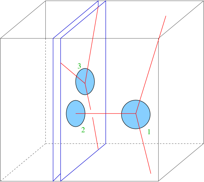
Figure 1: The picture of modern super-string theory contains closed strings which propagate in a 10D background, $p$-branes stretching along $p+1$-dimensional surfaces and open strings whose end-points move within the branes’ world-volume.

Such developments are the main focus of this lecture. To begin with, we shall take a much closer look at the various elements of Figure 1, enlarging them so that we can see the strings’ finite extension. In the process we shall learn how to model the picture in mathematical physics. This will involve the whole wealth of boundary conformal field theory (CFT), a domain that is also known for its beautiful applications to critical phenomena (see e.g. the lecture of Smirnov for some recent applications). As we scan over the picture of the world, we shall gradually set up a dictionary between its various elements and concepts of 2D boundary conformal field theory.

After this more introductory part we shall start to discuss some of the recent string inspired developments in boundary conformal field theory. Our presentation will follow the traditional devision into rational vs. non-rational conformal field theory. The former is relevant for the study of strings on compact components of the 10-dimensional world. This subject has seen an enormous boost in recent years and by now there exist very powerful techniques that are essentially universal, i.e. apply to very large classes of compact target spaces. Non-rational conformal field theory, on the other hand, is relevant for string theory in non-compact spaces. As we will discuss, such non-compact backgrounds are an essential ingredient in string theory duals of (large N) gauge theory. They are also vital for studies of time-dependent string backgrounds. Applications to these two domains have pushed non-rational conformal field theory to the forefront of research in string theory.

2 Strings, branes and boundary conformal field theory

The main purpose of this section is to zoom in on the elements of the picture we sketched above, to understand what they look like in full string theory and how they are modeled in mathematical physics.

2.1 Closed strings and bulk conformal field theory

The first element we are going to enlarge is a junction at which three closed strings come together (see Figure 2). Our aim here is to assign a number to this junction which we can interpret as an amplitude for the joining/splitting of closed strings. This number depends on the particular background we consider and on the states $\phi$ of the three closed strings that participate in the process. The latter decorate the three external legs of Figure 2 and they are taken from an infinite set of possible closed string modes. When we deal with strings in flat space, for example, states are characterized by a center of mass momentum and an infinite variety of different vibrational modes.

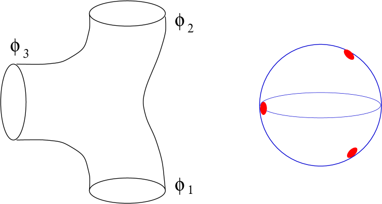
Figure 2: The interaction 3-vertex of three closed string modes $\Phi_{\nu}$ is obtained from a 3-point function of a 2D conformal field theory on a closed surface $\mathbb{P}^{1}$. The fundamental fields of the 2D conformal field theory arise through the parametrization of the closed string’s world-surface.

To assign an amplitude to the vertex, we consider the latter as an image of a 3-punctured 2-sphere ${\mathbb{P}^{1}}$ under the parametrization map $(X^{\mu}(z,\bar{z}))_{\mu=0,1,\dots,9}$. Being the parametrization of the closed string’s world-surface, $X^{\mu}$ are components of a 10-dimensional bosonic field with action

$$S_{\rm CS}[X]\ =\ S[X]\ =\ \frac{1}{4\pi\alpha^{\prime}}\,\int\,dzd{\bar{z}}\,\left(g_{\mu\nu}(X)+B_{\mu\nu}(X)\right)\,\partial X^{\mu}\bar{\partial}X^{\nu}\ +\ \dots$$ (21)

where the dots stand for additional terms e.g. involving Fermions. If our strings propagate in flat space then the background metric $g$ and B-field $B$ are constant. This implies that the action is quadratic and computations in the resulting free field theory can be reduced to Gaussian integrals. For more general backgrounds, however, both $g$ and $B$ depend on the coordinates of the background and we are dealing with (a special class of scale invariant) 2D non-linear $\sigma$-models. Our discussion here has brought us to the first entry in our dictionary: it is claimed that possible closed string backgrounds are associated with 2D conformal field theories on closed surfaces. Closed string modes $\phi$ correspond to fields $\Phi(z,{\bar{z}})$ in the conformal field theory. The 3-point functions of such fields are determined by conformal symmetry up to some constants

$$\langle\Phi_{1}(z_{1},{\bar{z}}_{1})\Phi_{2}(z_{2},{\bar{z}}_{2})\Phi_{3}(z_{3},{\bar{z}}_{3})\rangle\ =\ \frac{C(\phi_{1},\phi_{2},\phi_{3})}{|z_{12}|^{2\Delta_{12}}|z_{23}|^{2\Delta_{23}}|z_{13}|^{2\Delta_{23}}}$$

where $z_{ij}=z_{i}-z_{j}$ and the exponents $\Delta_{ij}$ are certain linear combinations of the scaling dimensions $\Delta_{i}$ of the fields $\Phi_{i}$. Along with the spectrum of these scaling dimensions $\Delta_{i}$, the 3-point couplings $C$ are known to contain all the information about the conformal field theory. They obey various consistency conditions which are rather difficult to solve, but starting from the seminal paper by Belavin et al.[9], many such solutions have been constructed. In string theory, the 3-point couplings $C$ provide the amplitude of the 3-point vertex, i.e. they tell us how likely it is that two closed string modes $\phi_{1},\phi_{2}$ combine into a single closed string in the mode $\phi_{3}$.

2.2 Branes and boundary conditions in CFT

Now that we understand how to model closed strings, let us start to look at the next element of Figure 1, namely at branes. Originally, the latter entered the image through the study of classical super-gravity. In fact, it is known for many years that the differential equations of classical super-gravity possess static solutions which describe charged and massive objects whose mass and charge is localized along certain $p+1$-dimensional hyper-surfaces. These objects are very much like extremal black holes, only that they extend in $p$ spatial directions. Since closed string theory is considered as an interesting candidate for a consistent short distance completion of gravity, we are lead to the obvious problem of finding a description for branes in string theory.

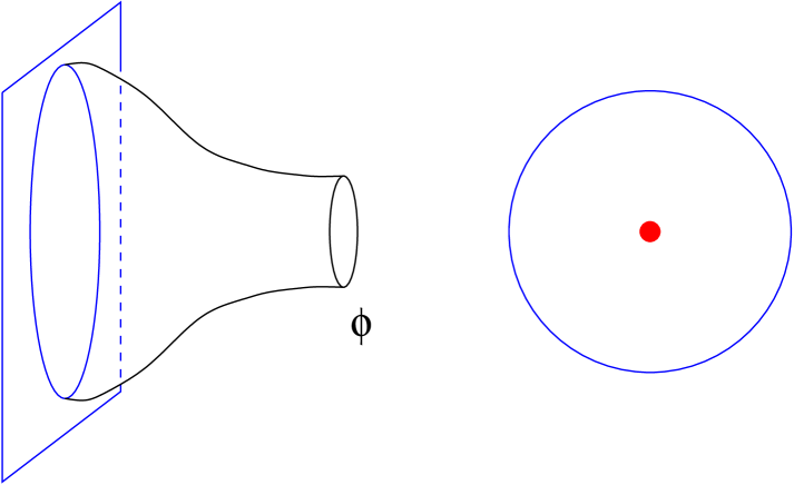
Figure 3: The interaction of closed strings with a brane is related to the bulk 1-point function in a 2D conformal field theory on a disc. Different branes correspond to different boundary conditions imposed along the boundary of the disk.

To answer this question let us now enlarge another element of our image (see Figure 3). We claimed above that branes are charged and massive objects. As such, they can interact with various other objects in the bulk, e.g. through exchange of gravitons and higher closed string modes. When such a closed string mode hits the brane or is emitted from it, we obtain the picture shown in Figure 3. The parametrization of the closed string world-surface now involves a map from a disc to the 10-dimensional background such that the boundary of the disc is embedded into the world-volume of the brane. We ensure this by imposing Dirichlet boundary conditions for all components of $(X^{\mu})$ which are associated with directions transverse to the brane. Our discussion here motivates the following general proposal that was first formulated by Polchinski[45]: branes in some closed string background correspond to conformally invariant boundary conditions of the associated conformal field theory. It is well known that boundary conditions in conformal field theory can be characterized by the 1-point functions of bulk fields $\Phi$. Using once more conformal invariance and a conformal mapping from the disc to the upper half-plane, the 1-point functions are easily shown to possess the following general form

$$\langle\Phi(z,{\bar{z}})\rangle^{\rm BC}\ =\ \frac{B^{\rm BC}(\phi)}{|z-{\bar{z}}|^{2\Delta_{\phi}}}\ \ .$$

In other words, conformally invariant boundary conditions are uniquely determined by the 1-point couplings $B(\phi)$. The latter provide a measure for how strongly a given closed string mode $\phi$ couples to the brane and hence in particular encodes information on the mass and charge of the brane.

2.3 Open strings and boundary fields

At this point we are still missing the open strings that we would expect to be around as soon as we introduce branes. This is indeed the case. To argue that open strings are indeed part of our present setup, a brief look at lattice spin models with boundaries may be helpful. The latter are closely related to the 2D continuum field theories we are dealing with. Moreover, it is intuitively obvious that such lattice systems contain a set of excitations which can only live along the boundary and which depend on the specific boundary condition we impose. In the 2-dimensional Ising model with free boundary conditions, for example, we can measure the boundary magnetization. Once we fix the boundary spins, however, measurements of this quantity become trivial and hence do not correspond to an observable of the model. In continuum field theory, boundary excitations are described by fields which can only be inserted at points along the boundary, i.e. to so-called boundary fields. These are exactly the objects that we need in order to model open strings. As in the case of closed strings, there exists an infinite number of open string modes $\psi$ and to these we assign boundary fields $\Psi(u)$ of the corresponding boundary conformal field theory. The spectrum of open string modes depends on the brane we consider, just as the spectrum of boundary fields depends on the boundary condition we impose along the boundary.

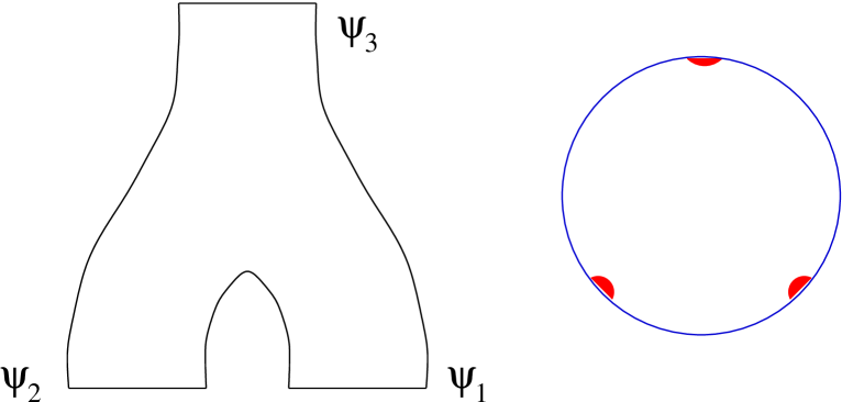
Figure 4: The interaction 3-vertex of open string modes $\Psi_{\nu}$ is obtained from a 3-point function of boundary fields in a 2D conformal field theory on the disc or half-plane.

There is one new set of couplings that comes with the vertex of three open string modes (see Figure 4). The computation of such a vertex involves a disc with three fields inserted along the boundary. Once more, this amplitude is determined by conformal invariance up to a set of 3-point couplings,

$$\langle\Psi_{1}(u_{1})\Psi_{2}(u_{2})\Psi_{3}(u_{3})\rangle\ =\ \frac{O(\psi_{1},\psi_{2},\psi_{3})}{|u_{12}|^{\Delta_{12}}|u_{23}|^{\Delta_{23}}|u_{13}|^{\Delta_{23}}}$$

where $u_{ij}=u_{i}-u_{j}$ and the $u_{i}$ are coordinates for the boundary of the upper half-plane. Needless to say that the 3-point couplings $O$ encode the probability of two open string modes $\psi_{1},\psi_{2}$ to combine into a single open string in the mode $\psi_{3}$.

This concludes our journey through the various elements of Figure 1. Along the way we have learned to characterize boundary conformal field theories through three different sets of couplings, the 3-point couplings $C$ of the bulk fields, the couplings $B$ appearing in the 1-point function of bulk fields and the 3-point couplings $O$ of boundary fields. This is a rather abstract way to think about boundary conformal field theories, especially when compared with the action (21) for closed strings that we started our discussion with. Since it is sometimes helpful to think about conformal field theories in terms of such actions, we would like to mention that in the case of open strings, $S[X]$ gets modified to

$$S_{\rm OS}[X]\ =\ S[X]+\frac{1}{2\pi{\alpha^{\prime}}}\,\int_{\partial\Sigma}du\,A_{\mu}(X)\,\partial_{u}X^{\mu}(u)$$ (22)

where the first term is the same as in formula (21) with $\Sigma$ being replaced by a surface with boundary. The new boundary term means that open strings can couple through the velocity $\partial_{u}X^{\mu}$ of their endpoints to a new background field, namely to a vector field $A_{\mu}(X)$. We interpret $A$ as a gauge field on the brane and think of the string endpoints as carrying charges. The action (22) is to be supplemented by Dirichlet boundary conditions on $X$ for all directions transverse to the brane.

2.4 Instabilities, dynamics and RG-flows

In the last three subsections, our dictionary has received quite a number of entries, but there are a few more that we would like to add in passing. To motivate these additional entries, we note that many of the existing string backgrounds are actually unstable. This applies e.g. to the 26-dimensional bosonic string theory and it is a common phenomenon in the context of branes. In fact, configurations of several stable branes tend to be unstable, the most famous example being the pair of a brane and its anti-brane.

In general relativity we can easily detect instabilities of some given static solution to the classical field equations. All we need to study is the spectrum of fluctuations around the solution. Modes that are exponentially enhanced are associated with instabilities. Let us now see how we can find unstable modes in string theory. To this end we consider some static background. Its conformal field theory description involves a product of a time-like free field $X^{0}$ and a unitary conformal field theory whose target is the 9-dimensional spatial slice of the static background. This theory possesses an exponentially growing mode if we can add the following conformally invariant terms to the action

$$\delta S\ \sim\ \int_{\Sigma}dzd{\bar{z}}\ e^{\epsilon_{\Phi}X^{0}(z,{\bar{z}})}\,\Phi(z,{\bar{z}})+\int_{\partial\Sigma}du\ e^{\epsilon_{\Psi}X^{0}(u)}\,\Psi(u)$$ (23)

where $\Phi(z,{\bar{z}})$ and $\Psi(u)$ are bulk and boundary fields in the conformal field theory for the spatial slice and the coefficients $\epsilon_{\Phi}$ and $\epsilon_{\Psi}$ must be real in order to have an exponential growth with time. But such exponential fields of a time-like free boson possess a positive scaling dimension so that the fields $\Phi$ and $\Psi$ must have scaling dimensions $\Delta_{\Phi}\leq 2$ and $\Delta_{\Psi}\leq 1$ if we want $\delta S$ to be scale invariant. In other words, instabilities of a closed string background and branes therein correspond to relevant bulk and boundary fields, respectively.

If we wanted to control the full decay process generated by an instability, we would have to solve the theory with interaction $\delta S$. At present, no example of such a theory has been constructed within 10D string theory. Nevertheless, some insights into aspects of decay processes have been obtained using a proposed relation with renormalization group (RG) flows. This requires, however, that we reduce our ambitions and only try to identify the final state of the decay process rather than the whole dynamical evolution. Let us consider an initial state which is encoded in a CFT₁ for the 9-dimensional spatial slice of the static background. Next we choose some relevant bulk or boundary field $\Phi$ or $\Psi$ to trigger the decay. After all radiation has has escaped, we expect our system to settle down in a static final state that is again described by a product of a time-like free boson and a CFT₂ for the spatial slice of the final stable state. Hence, the dynamics has lead us from some CFT₁ to CFT₂ with the help of relevant fields $\Phi$ or $\Psi$. It is obviously tempting to think that CFT₂ is the IR fixed point of the RG flow from CFT₁ on the RG trajectory that is generated by adding $\Phi$ or $\Psi$. Supporting evidence for this proposal is strong in the case of boundary instabilities, but the proposal seems much harder to justify when we deal unstable bulk theories. A more thorough discussion of these issues and many further references can be found in the literature[27].

2.5 Summary: dictionary between ST and BCFT

Let us pause for a moment and review all the entries in our dictionary between string theory and 2D boundary conformal field theory:
                Closed string background ${\mathcal{X}}$ 2D CFT ${\mathcal{C}}_{{\mathcal{X}}}$ on closed surface $\Sigma$ Closed string mode $\phi$ Bulk field $\Phi(z,{\bar{z}}),z\in\Sigma,$ in ${\mathcal{C}}_{\mathcal{X}}$ Closed string vertex $C$ 3-point function of bulk fields Brane ${\mathcal{B}}$ in background Boundary condition (BC) for ${\mathcal{C}}_{\mathcal{X}}$ $\Rightarrow$ BCFT ${\mathcal{C}}_{{\mathcal{X}}}^{\mathcal{B}}$ on open surface $\Sigma$ Open string mode $\psi$ Boundary field $\Psi(u),u\in\partial\Sigma,$ in ${\mathcal{C}}_{\mathcal{X}}^{\mathcal{B}}$ Open string vertex $O$ 3-point function of boundary fields Instability of a background Relevant bulk- or boundary-field Initial/final state of decay UV/IR fixed point of an RG-flow
Recall that the last line has the status of a conjecture. To test our dictionary one may form sentences in string theory (or gravity) and check that they translate into meaningful sentences of (boundary) conformal field theory.

3 Rational BCFT and strings in compact backgrounds

We are now prepared to begin reviewing results on the explicit construction of boundary conformal field theories. Systematic rational conformal field theory model building usually starts with theories whose target space is a compact group manifold $G$. It then proceeds to cosets and orbifolds. Among them one finds all known models with interesting applications to statistical physics and string theory. Here we shall explain the most central results of the field using one special example, namely the group $G=$SU(2)$\cong S^{3}$. A few comments on various generalizations and extensions are collected at the end.

3.1 Strings on the 3-sphere

Before we look at strings moving on a 3-sphere, let us recall that, to leading order in ${\alpha^{\prime}}$, $\sigma$-models of the form (21) are conformal invariant if the background fields satisfy

$${\alpha^{\prime}}{\mathcal{R}}_{\mu\nu}(g)-\frac{{\alpha^{\prime}}}{4}H_{\mu\lambda\omega}H_{\nu}^{\ \lambda\omega}\ =\ O({\alpha^{\prime}}^{2})\ \ .$$

Here, ${\mathcal{R}}$ is the curvature of the background metric $g$ and $H=dB$. Hence, if strings move in a curved background, then a non-vanishing magnetic field $B$ is unavoidable.

With this in mind let us consider strings on a 3-sphere $S^{3}\cong$ SU(2). Their world-surfaces are parametrized by a group valued map $h:\Sigma\rightarrow$ SU(2) and these parametrization fields appear in an action of the form

$$S[h]\ =\ \frac{{\sf k}}{4\pi}\int dzd{\bar{z}}\ {\rm tr\ }(h^{-1}\partial h)(h^{-1}\bar{\partial}h)+\frac{{\sf k}}{12\pi}\int d^{-1}(h^{-1}dh)^{\wedge_{3}}\ \ .$$ (31)

The second term is known as the Wess-Zumino-Witten (WZW) term. Locally, it may be rewritten in the form of the second term in eq. (21). We also note that the parameter ${\sf k}$ is a measure for the size of the 3-sphere and that, in the quantum theory, ${\sf k}$ must be integer.

The WZW model possesses a large symmetry, given by two commuting actions of the affine Lie algebra ${\widehat{{\rm su}}(2)}_{\sf k}$. Each of these two algebras is generated by the Laurent modes $J^{\mu}_{n},n\in\mathbb{Z},$ of an su(2)-valued conserved current $J=J^{\mu}t_{\mu}$ with relations

$$[\,J^{\mu}_{n}\,,\,J^{\nu}_{m}\,]\ =\ i{f^{\mu\nu}}_{\rho}\,J^{\rho}_{n+m}+{{\sf k}}\,n\,\delta^{\mu,\nu}\,\delta_{n,-m}\ \ .$$ (32)

The two affine Lie algebras act on the space of fields in the theory, extending the actions that are induced by the usual left and right translation of the group on itself.

It turns out that a wide class of boundary conformal field theories can be written down in terms of data from the representation theory of their infinite dimensional symmetries. The most important such data are the set ${\mathcal{J}}$ of unitary representations, the so-called modular $S$-matrix, the Clebsch-Gordan multiplicities $N$ of the fusion product and an infinite dimensional generalization of the 6J-symbols which is known as the Fusing matrix $F$. For the SU(2) affine Lie algebra, explicit formulae may be spelled out. In this case, the requirement of unitarity leaves us with just a finite number of representations. We label them through $j\in{\mathcal{J}}=\{0,1/2,\dots,{\sf k}/2\}$. Their conformal weights are given by $\Delta_{j}=j(j+1)/({\sf k}+2)$ and for the modular S-matrix one finds

$$S_{ij}\ =\ \sqrt{\frac{2}{{\sf k}+2}}\ \sin\frac{\pi(2i+1)(2j+1)}{{\sf k}+2}\ \ .$$ (33)

With the help of the Verlinde formula it is not difficult to compute the following fusion rules $N$ from the modular S-matrix,

$${N_{ij}}^{k}\ =\ \left\{\begin{array}[]{ll}1&\mbox{ for }\ k=|i-j|,\dots,{\mbox{\rm min\/}}(i+j,{\sf k}-i-j)\\[5.69054pt] 0&\mbox{ otherwise }\end{array}\right.\ \ .$$ (34)

They are similar to the Clebsch-Gordan multiplicities of the Lie algebra su(2), apart from the truncation which appears whenever $i+j>{\sf k}/2$.

Formulae for the fusing matrix also exist in the literature. Since they are a bit more involved, we shall not present them here. Let us only mention one property concerning their limiting behavior as we send ${\sf k}\rightarrow\infty$,

$$\lim_{{\sf k}\rightarrow\infty}F_{{\scriptstyle J}{\scriptstyle k}}\hskip 0.85358pt\displaystyle{[}\hskip 1.42262pt\begin{array}[]{ll}{\scriptstyle i}&{\scriptstyle j}\\[-4.2679pt] {\scriptstyle I}&{\scriptstyle K}\end{array}\displaystyle{]}\ =\ \displaystyle{\{}\hskip 1.42262pt\begin{array}[]{lll}{\scriptstyle i}&{\scriptstyle j}&{\scriptstyle k}\\[-4.2679pt] {\scriptstyle I}&{\scriptstyle J}&{\scriptstyle K}\end{array}\displaystyle{\}}\ \ .$$ (35)

This concludes our list of representation theoretic data for the affine Lie algebra. We shall see these quantities again in a moment when we write down formulae for the couplings $B$ of closed strings to branes on $S^{3}$, for their open string spectra and the 3-point vertices $O$ of open string modes.

3.2 Branes on group manifolds

Many constructions of conformal invariant boundary theories are ultimately based on fundamental observations made by J. Cardy[13]. When applied to the case at hand, they provide us with a finite set of ${\sf k}+1$ boundary conformal field theories which we label by $J=0,1/2,\dots,{\sf k}/2$, just as we enumerate the unitary representations of the corresponding affine Lie algebra. Recall that these boundary theories can be uniquely characterized through the couplings $B$ that appear in the 1-point functions of the bulk fields. According to Cardy’s solution, these 1-point couplings are simply given by the matrix elements of the modular S-matrix,

$$\langle\Phi_{j}^{ab}(z,{\bar{z}})\rangle_{J}\ =\ \frac{S_{Jj}}{\sqrt{S_{0}j}}\ \frac{\delta^{a,b}}{|z-{\bar{z}}|^{2\Delta_{j}}}$$ (36)

where $\Delta_{j}=j(j+1)/({\sf k}+2)$. The superscripts $a,b=-j,\dots,j,$ placed at the symbol $\phi$ label different components within a tensor multiplet $\phi_{j}$. One should think of these labels as the quantum numbers for ground states of the closed string. They are the same labels that appear on the matrix elements $D^{j}_{ab}(g)$ of group representations, except that the label $j$ is cut off at $j\leq{\sf k}/2$.

Geometrically, these boundary theories were found[3] to describe branes that are localized along a discrete set of conjugacy classes of SU(2), i.e. along 2-spheres around the group unit $e\in$ SU(2). They come equipped with a magnetic field of the form

$$B\ \sim\ {\rm tr\ }h^{-1}dh\,\wedge\,\frac{{\rm Ad}_{h}+1}{{\rm Ad}_{h}-1}\,h^{-1}dh\ \ ,$$ (37)

where ${\rm Ad}$ denotes the adjoint action of the group on its Lie algebra. For higher groups $G$, such a field $B$ gives a non-trivial potential for the pull-back of the WZW 3-form to the branes’ world-volumes. Such 2-form potentials on conjugacy classes of a group $G$ were considered in the mathematical literature. There they appear in connection with deformations of the theory of co-adjoint orbits.

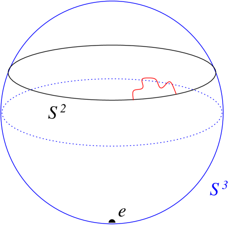
Figure 5: Maximally symmetric branes on a 3-sphere are localized along conjugacy classes of SU(2), i.e. they are either point-like or they wrap a 2-sphere in $S^{3}$. Such spherical branes exist only for a discrete set of radii.

Our geometrical interpretation of the boundary theories with 1-point functions (36) may be justified in several different ways. The argument we want to give here is based on the observation[21]

$$\langle\Phi^{ab}_{j}(z,{\bar{z}})\rangle_{J({\sf k})}\ \stackrel{{\scriptstyle{\sf k}\rightarrow\infty}}{{\sim}}\ \int_{\rm SU(2)}d\mu(g)\,\delta(\vartheta(g)-\vartheta_{0})\,\phi^{ab}_{j}(g)\ \ ,$$ (38)

where $d\mu(g)$ denotes the Haar measure on SU(2), $\phi_{j}^{ab}(g)\sim D^{j}_{ab}(g)$ are the wave functions of the lightest closed string modes and $\vartheta$ is the azimuthal angle on the 3-sphere. In taking the limit, we allowed the boundary label $J$ to depend on the level ${\sf k}$ and we defined $\vartheta_{0}:=2\pi\lim J({\sf k})/{\sf k}$. Since $0\leq J\leq{\sf k}/2$, the angle $\vartheta_{0}$ lies in the interval $[0,\pi]$. The appearance of the $\delta$-function on the right hand side shows that closed string modes indeed detect a spherical object which is localized at the azimuthal angle $\vartheta=\vartheta_{0}$.

3.3 Open strings on group manifolds

Let us now turn to the open strings which can propagate along the ${\sf k}+1$ different spherical branes on $S^{3}$. According to our dictionary, this means that we want to obtain the set of boundary fields and the 3-point couplings $O$ for each of the above boundary theories. Following general arguments, it is possible to show that the space of boundary fields carries the action of a single affine Lie algebra rather than two commuting actions as in the case of bulk fields. This reflects a similar reduction of the geometric symmetries: whereas there exist two commuting sets of (left and right) translations on SU(2), only a special combination, namely the adjoint action, leaves the conjugacy classes invariant. Under the action of the affine Lie algebra ${\widehat{{\rm su}}(2)}_{\sf k}$, the space ${\mathcal{H}}_{J}$ of boundary fields decomposes as

$${\mathcal{H}}_{J}\ =\ {\mathcal{H}}_{JJ}\ =\ {\bigoplus}_{j}\ {N_{JJ}}^{j}\ {\mathcal{V}}_{j}$$ (39)

where ${\mathcal{V}}_{j}$, $j=0,1/2,\dots,{\sf k}/2$, denote irreducible unitary representations of the affine Lie algebra ${\widehat{{\rm su}}(2)}_{\sf k}$, and where ${N_{JJ}}^{j}$ are the associated fusion rules (see eq. (34)). Note that only integer spins $j$ appear on the right hand side of eq. (39) and that in the limit ${\sf k}\rightarrow\infty$, the summation on the right hand side is truncated at $j_{max}=2J$. This means that the decomposition of ${\mathcal{H}}_{J}$ is as close as it can be to the decomposition of ${\mbox{\rm Mat}}(2J+1)$ into su(2) multiplets. In fact, there is a correspondence between the spin $j$ multiplets of matrices ${\it Y}^{j}_{a}\in{\mbox{\rm Mat}}(2J+1)$ and ground states in ${\mathcal{V}}_{j}\subset{\mathcal{H}}_{J}$. It is also worth pointing out the similarity between the labeling of open string ground states and spherical harmonics $Y_{a}^{j}(\varphi,\theta)$. Only the cut-off at $j_{max}=2J$ on the spin $j$ does not appear for functions on a 2-sphere.

Boundary fields $\psi^{a}_{j}$ associated with ground states of the open string are labeled by the representation $j=0,1,\dots,j_{max}$ and $a=-j,\dots,j$. Their 3-point vertices were found[4] using important previous work by Runkel[53] on minimal models,

$$\langle\Psi^{a}_{i}(u_{1})\,\Psi_{j}^{b}(u_{2})\,\Psi_{k}^{c}(u_{3})\rangle_{J}\ =\ {|u_{12}|^{-\Delta_{12}}|u_{23}|^{-\Delta_{23}}|u_{13}|^{-\Delta_{23}}}\,\displaystyle{[}\,\begin{array}[]{lll}{\scriptstyle i}&{\scriptstyle j}&{\scriptstyle k}\\[-5.69054pt] {\scriptstyle a}&{\scriptstyle b}&{\scriptstyle c}\end{array}\displaystyle{]}\,F_{{\scriptstyle J}{\scriptstyle k}}\hskip 0.85358pt\displaystyle{[}\hskip 1.42262pt\begin{array}[]{ll}{\scriptstyle j}&{\scriptstyle i}\\[-4.2679pt] {\scriptstyle J}&{\scriptstyle J}\end{array}\displaystyle{]}$$ (310)

where the symbol in square brackets stands for the Clebsch-Gordan coefficients of su(2). The latter guarantee that both sides of the equation transform in the same way under the action of the zero mode algebra su(2). The non-trivial part of equation (310) therefore concerns the relation of 3-point vertices for open strings with entries of the Fusing matrix.

We conclude this subsection with a brief remark on an interesting link to non-commutative geometry. Let us observe that the 3-point couplings simplify significantly if we send ${\sf k}$ to infinity,

$$\langle\Psi^{a}_{i}(u_{1})\,\Psi_{j}^{b}(u_{2})\,\Psi_{k}^{c}(u_{3})\rangle_{J}^{{\sf k}\rightarrow\infty}\,=\,\displaystyle{\{}\hskip 1.42262pt\begin{array}[]{lll}{\scriptstyle j}&{\scriptstyle i}&{\scriptstyle k}\\[-4.2679pt] {\scriptstyle J}&{\scriptstyle J}&{\scriptstyle J}\end{array}\displaystyle{\}}\,\displaystyle{[}\,\begin{array}[]{lll}{\scriptstyle i}&{\scriptstyle j}&{\scriptstyle k}\\[-5.69054pt] {\scriptstyle a}&{\scriptstyle b}&{\scriptstyle c}\end{array}\displaystyle{]}\ \ .$$ (311)

Here we have used the property (35) of the fusing matrix. It is straightforward to check that the numbers appearing on the right hand side of this equation arise naturally from the multiplication of ordinary $(2J+1)\times(2J+1)$ matrices. In fact, the same numbers appear when we rewrite the product ${\it Y}^{i}_{a}\cdot{\it Y}^{j}_{b}$ as a linear combination of the su(2) multiplets ${\it Y}^{k}_{c}\in{\mbox{\rm Mat}}(2J+1)$. In this sense, the 3-point vertices for open strings on branes in SU(2) provide an infinite dimensional deformation of matrix multiplication. The emergence of non-commutative matrix algebras in the context of open string theory is not surprising. As we have stressed before, the end-points of open strings behave like charged particles which can couple to the vector potential $A$ of the magnetic field on the brane. Hence, the non-commutativity we encounter in the context of open strings is directly related to a similar phenomenon for e.g. electrons in a strong magnetic field. Relations between branes, open string and non-commutative geometry were initially discovered for branes in flat space[16, 14, 55] and they have been studied extensively for several years.[59, 17]

3.4 Brane dynamics on group manifolds

Before we list a few generalizations of the above results, we would like to briefly comment on some dynamical processes involving branes in $S^{3}$. Here we shall use the conjectured relation with RG-flows in the 2D boundary conformal field theory. It turns out that the study of boundary renormalization groups flows in models with an SU(2) current algebra is a classical problem of mathematical physics that was first addressed in the context of the Kondo-model.

The Kondo-model is designed to understand the effect of magnetic impurities on the low-temperature conductance properties of a 3D conductor. The latter can have electrons in a number ${\sf k}$ of conduction bands. If the impurities are far apart, their effect may be understood within an s-wave approximation of scattering events between a conduction electron and the impurity. This allows to formulate the whole problem on a 2-dimensional world-sheet for which the coordinates $(u,v)$ are associated with the time and the radial distance from the impurity, respectively. One can build several currents out of the basic fermionic fields. Among them is a spin current $\vec{J}(u,v)$. Its Laurent modes satisfy the relations (32) of a $\widehat{\rm su}(2)_{\sf k}$ current algebra. This spin current is the one that couples to the magnetic impurity of spin $J_{M}$ which is sitting at the boundary $v=0$,

$$S_{\rm Kondo}\ \sim\ \lambda\int_{-\infty}^{\infty}du\,\Lambda_{\mu}J^{\mu}(u,0)\ \ .$$ (312)

Here, the matrices $\Lambda_{\mu},\mu=1,2,3$ form a $(2J_{M}+1)$-dimensional irreducible representation of su(2) and the parameter $\lambda$ controls the strength of the coupling. Note that the term (312) is identical to the coupling of open string ends with velocity $J^{\mu}(u,0)$ to a background gauge field $A_{\mu}=\Lambda_{\mu}$ (see formula (22)). Hence, $\Lambda_{\mu}$ may be interpreted as a constant non-abelian gauge field on one of our branes. For $M>1$, the interaction is marginally relevant so that, according to the proposal formulated in subsection 2.4, switching on such non-abelian gauge fields represents an instability. Its effect on the brane can be understood by searching for an RG fixed-point along the RG trajectory generated by the term (312).

Fortunately, a lot of techniques have been developed to deal with perturbations of the form (312). From the old analysis it is known that non-trivial fixed points are reached at a finite value $\lambda=\lambda^{*}$ of the renormalized coupling constant $\lambda$ if $2J_{M}\leq{\sf k}$ (exact- or over-screening resp.). These fixed points have been identified through several different approaches and a simple rule summarizing the results of such investigations was formulated by Affleck and Ludwig[1]. The latter can be applied directly to our branes on SU(2)[22] and it shows that e.g. point-like branes carrying a constant U(M) gauge field decay into an extended spherical brane with label $J_{M}=(M-1)/2$.

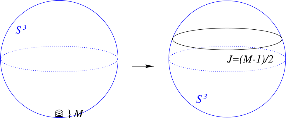
Figure 6: Studies of RG flows in models with a SU(2) current symmetry show that point-like branes carrying a constant U(M) gauge field decay into an extended spherical brane with label $J_{M}=(M-1)/2$.

For large values of ${\sf k}$, the result we have just formulated admits an easier derivation using some of the geometric structures we have outlined above. It is widely known that massless open string modes give rise to a gauge theory on the brane to which they are attached. But due to the presence of the $B$-field on our spherical branes, the open strings detect a non-commutative (matrix) geometry (cf. last subsection). Hence, we are tempted to conclude that a special non-commutative gauge theory should be associated with branes on the 3-sphere. This is indeed the case and the precise form of the relevant gauge theory has been determined following the usual rules of string theory[5], at least to leading order in $\alpha^{\prime}$. Once the action of this gauge theory is found, one can search for instabilities and classical ground states. The outcome of such an analysis confirms very nicely the formation of spherical branes from point-like branes that we have described in our discussion of RG-fixed points above. This agreement is not accidental. In fact, when ${\sf k}$ is large, the action of the non-commutative field theory is a functional on the space of boundary couplings whose stationary points approximate zeros of the $\beta$-function. The analysis of RG-fixed points through non-commutative field equations has significant technical advantages over more traditional approaches. These are related to a very efficient book-keeping of the possible boundary couplings through non-commutative variables.

3.5 Overview: various generalizations and extensions

The material presented in this section has been generalized in many different directions and we would like to list a few of these developments before we leave the rational boundary conformal field theories. Not surprisingly, results similar to the ones we have reviewed here are also available for all other compact simple simply connected Lie groups. For many of the higher groups, moreover, there exist new families of maximally symmetric branes that are associated with outer automorphisms of $G$ and hence have no analogue in the case of SU(2). Their boundary couplings $B$ and open string spectra were first studied by Felder et al.[21] (see also [43, 25]). Results on the open string couplings and dynamics have also been obtained[6]. In addition to the maximally symmetric branes, i.e. those that admit an action of the whole group $G$, one can impose boundary conditions which break part of this symmetry. Investigations of such branes were initiated in a paper by Moore et al.[39] and a rather systematic construction has been developed more recently[50]. It is worth mentioning that symmetry breaking branes on group manifolds possess interesting applications to defect lines in 2D conformal field theory. With the theory of strings and branes on group manifolds being under such good control, one can start to descend to orbifolds and cosets thereof. Studies of branes and open strings in curved orbifold backgrounds possess a long history[49, 10, 42, 24, 11]. The theory of branes in coset models has also been treated by many authors (see e.g. [39, 26, 19, 23] for some early contributions and references).

4 Recent progress for strings in non-compact spaces

The last part of this lecture is devoted to some developments in the area of non-rational boundary conformal field theory. As indicated in the introduction, these are highly relevant for the study of dualities between string and gauge theory and for time-dependent processes in string theory. Here we shall explain these motivations in some detail and then focus mainly on one particular model, namely on the Liouville field theory.

4.1 String/gauge theory dualities

According to an old observation by ’t Hooft, structures found in closed string amplitudes are very reminiscent of features in the perturbative expansion of large $N$ gauge theories. This suggests that it might be possible to compute gauge theory amplitudes from string theory. Though the idea has been around for a long time, only a single concrete example was known until 1997: The duality between the quantum mechanics of hermitian matrices and a toy model of string theory with a 2-dimensional target space (see e.g. the lectures of Klebanov[31] and references therein).

After branes had entered the stage of string theory, the situation changed drastically. We may grasp the fundamental role of branes for such developments through the following short analysis of Figure 7. The image shows a simple string diagram that admits two rather distinct interpretations. We can either think of a process in which a closed string mode is emitted from one brane and propagates a distance $\Delta x$ through the background before being absorbed by a second brane. Alternatively, the process can be seen as a pair creation and subsequent annihilation of open strings which end on the two involved branes. Though none of these interpretations is distinguished a priori, actual computations may favor one of them, depending on the separation $\Delta x$ between the branes. If they are very far apart only the massless closed string modes contribute significantly to the amplitude and hence one can safely perform the string theory computation in its super-gravity approximation. For short distances $\Delta x$ between the branes, however, many massive closed string modes start to enter the computation and we better switch to a description in terms of light, i.e. mildly stretched, open strings. This reinterpretation leaves us with a one-loop computation in the gauge theory of massless open string modes. The reasoning we have just gone through hints toward an intimate relation between closed string models and gauge theory. This relation has a few interesting features. Observe, for example, that it does not preserve the underlying space-time dimensions since closed strings propagate in the 10D background while gauge bosons cannot leave the branes’ $p+1$-dimensional world-volume. In addition, the relation also mixes different loop orders as can be inferred from Figure 7. Here, we found a closed string tree level amplitude that contains information about a gauge theory one-loop diagram.

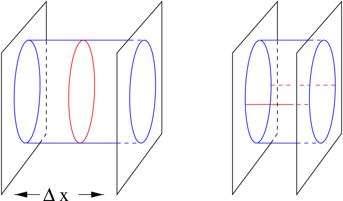
Figure 7: Depending on the distance $\Delta x$ between branes the shown string amplitude can be approximated by either a tree level computation in super-gravity or a one-loop gauge theory computation.

With all this in mind it seems no longer surprising that branes provide us with many new and concrete dualities between gauge theories and models of closed strings. The most famous example certainly is Maldacena’s duality[35] between ${\mathcal{N}}=4$ Super-Yang-Mills theory and string theory on $AdS_{5}\times S^{5}$. It involves an SU(N) gauge theory at large N with ’t Hooft coupling $\lambda=g_{\rm YM}N^{2}$ on one side and an $AdS_{5}$ space with curvature radius $R^{2}/{\alpha^{\prime}}\sim\sqrt{\lambda}$ on the other. Hence, if we want to study gauge theory at finite ’t Hooft coupling, the curvature of $AdS_{5}$ cannot be neglected so that string effects become important. Not only does this bring us back to the main theme of the lecture, it also hides novel challenges arising from the fact that the relevant closed strings propagate on a non-compact curved background. Similar observations can be made for all the other known examples of such dualities between gauge and string theory[2]. Therefore, extending the methods and results reviewed in the previous section to non-compact target spaces becomes an important new task for conformal field theory.

Here we shall restrict our attention to the example of Liouville theory. Since it appears as constituent of 2D string theory, Liouville theory enters one side of the aforementioned duality with matrix quantum mechanics. More recent developments show that even this duality, though it pre-dates the discovery of branes in string theory by several years, ultimately arises is the same way as all the modern AdS/CFT-type dualities.

4.2 Liouville theory and its applications

Liouville theory may be considered as the minimal model of non-rational conformal field theory. It describes the motion of strings in a single direction with an exponential potential

$$S_{L}[X]\ \sim\ \int_{\Sigma}dzd{\bar{z}}\,\left(\partial X\bar{\partial}X+\mu e^{2bX}\right)\ \ .$$ (41)

Here, $X$ is a free bosonic field with background charge (linear dilaton). Note that a change of the parameter $\mu$ can be re-absorbed in a constant shift of the field $X$. Hence, the dependence of Liouville theory on $\mu$ is rather trivial. On the other hand, the correlation functions of the model display a very non-trivial dependence on the second parameter $b$. If we send $b$ to zero while rescaling $x=bX$ and $\lambda=b^{2}\mu$, we recover a model of particles in the potential $V(x)=\lambda\exp 2x$. The full field theoretic model contains both perturbative and non-perturbative corrections to this limit. The latter turn out to render the quantum theory self-dual with respect to the replacement $b\rightarrow b^{-1}$.

After these remarks on the model itself, let us briefly comment on two interesting applications. It is well known that a flat space with trivial background fields must be 26-dimensional for bosonic strings to propagate in it. This restriction to 26 dimensions, however, may be circumvented through the presence of non-trivial background fields. An example realizing such a scenario is the famous 2D string theory. It is constructed from a product of a 1-dimensional free bosonic field with Liouville theory at $b=1$. Obviously, such a closed string theory is of little practical interest, but is provides a valuable toy model for bosonic string theory. Compared to its 26-dimensional relative, the 2-dimensional model has the advantage of being perturbatively stable.

The second application is much more recent and also less well tested. It has been proposed[28] that a time-like version of Liouville theory at $b=i$ describes the homogeneous condensation of a closed string tachyon. A short look at the classical action (23) makes this proposal seem rather plausible. Recall that actions of this form describe a tachyon decay with a closed/open string tachyon profile $\Phi/\Psi$. If we consider a closed string tachyon which decays homogeneously, then we must choose $\Phi=\mu=$const. In addition, the parameter $\epsilon_{\phi}$ is now forced to be $\epsilon_{\mu}=2$ so that the interaction term (23) becomes scale invariant. After a Wick-rotation of the field $X^{0}=iX$, the interaction term looks formally like the interaction term in Liouville theory, only that the we have $b=i$, just as it was claimed above. Though on first sight this may all seem rather convincing, there are many subtleties hidden in the relation between Liouville theory and tachyon condensation. We will be able to display them more clearly once we have presented the exact solution of Liouville theory.

4.3 The solution of Liouville field theory

The solution of Liouville theory on closed and open surfaces has been a major success of the last ten years. We shall briefly spell out some of the most central formulae before we return to the applications.

Let us begin with a few simple remarks on the spectrum of the model. It is rather obvious that ground states $\phi_{P}$ of closed strings in the exponential potential can be labeled by a real number $P\geq 0$ which corresponds to the momentum of an incoming wave in the region $X\rightarrow-\infty$ where the potential vanishes. The states $\phi_{P}$ are stringy analogues of the particle wave functions

$$\varphi_{P}(x)\ =\ (\lambda/4)^{-i\omega}\,\Gamma^{-1}(-2i\omega)\,K_{2i\omega}(\sqrt{\lambda}e^{x})$$

for a Schroedinger problem in an exponential potential. Here, $K$ denotes the modified Bessel function of second kind. Finding the 3-vertex of the closed string modes $\phi_{P}$ turned out to be a very difficult problem that was only solved in 1994. The answer is usually expressed in terms of $\alpha_{j}=Q/2+iP_{j}$ where $Q=b+b^{-1}$,

$$C(\alpha_{1},\alpha_{2},\alpha_{3})\ =\ \left[\pi\mu\gamma(b^{2})(b^{2})^{1-b^{2}}\right]^{(2\tilde{\alpha}-Q)/b}\ \frac{\Upsilon^{\prime}(0)}{\Upsilon(2\tilde{\alpha}-Q)}\ \prod_{j=1}^{3}\,\frac{\Upsilon(2\alpha_{j})}{\Upsilon(2\tilde{\alpha}_{j})}\ \ .$$ (42)

Here, we have also introduced the notation $\tilde{\alpha}=(\alpha_{1}+\alpha_{2}+\alpha_{3})/2$ and $\tilde{\alpha}_{j}=\alpha-\alpha_{j}$. In addition, the special function $\Upsilon$ is obtained from Barnes’ double Gamma function by

$$\Upsilon(\alpha)\ :=\ \Gamma^{-1}_{2}(\alpha|b,b^{-1})\,\Gamma^{-1}_{2}(Q-\alpha|b,b^{-1})\ \ .$$ (43)

The solution (42) was first proposed by H. Dorn and H.J. Otto [15] and by A. and Al. Zamolodchikov [66], based on extensive earlier work by many authors (see e.g. the reviews [58, 63] for references). Crossing symmetry of the conjectured 3-point function was then checked analytically in two steps by Ponsot and Teschner [46] and by Teschner [63, 64].

Different conformally invariant boundary conditions were found and studied in several papers[20, 62, 67]. As one might suspect, there exist two different types of boundary theories, one describing point-like objects, the other corresponding to space-filling branes with an additional exponential boundary interaction that is felt by the end-points of open strings. It turns out that a point-like brane can only sit in the region where the Liouville potential $V$ becomes large. The simplest such brane is characterized by a 1-point coupling of the form

$$B(P)\ =\ \left(\pi\mu\gamma(b^{2})\right)^{-iP/b}\,\frac{2^{7/4}i\pi P}{\Gamma(1-2iPb^{-1})\Gamma(1-2iPb)}\ \ .$$ (44)

Open strings on this brane possess a discrete spectrum without continuous zero modes, in agreement with our geometrical intuition (see [67] for details). Let us remark that the brane with boundary coupling (44) is only one in an infinite set which is parametrized by two positive integers $(n,m)$. The status of the boundary conditions with $(n,m)\neq(1,1)$ as physical branes in Liouville theory, however, is less clear.

Extended branes in the Liouville background, on the other hand, obviously possess one continuous physical parameter. It enters the theory through an additional boundary interaction of the form $V_{B}\sim\mu_{B}\exp bX$. Note that constant shifts of the field $X$ have been used before to rescale the bulk parameter $\mu$. Hence, there is no freedom left now to absorb the new boundary parameter $\mu_{B}$. Consequently, coupling constants of the boundary theory display a non-trivial dependence on $\mu_{B}$ as can be seen in the case of the bulk 1-point coupling,[20]

$$B_{s}(P)\ =\ \left(\pi\mu\gamma(b^{2})\right)^{-iP/b}\,\cos(2\pi sP)\,\frac{\Gamma(1+2iPb^{-1})\Gamma(1+2iPb)}{-2^{5/4}i\pi P}\ \ .$$ (45)

Here, the parameter $s$ is related to the boundary coupling $\mu_{B}$ by the relation

$$\mu_{B}^{2}\sin\pi b^{2}\ =\ \mu\cosh^{2}\pi sb\ \ .$$

Each of these extended branes comes with a continuous spectrum of open string modes. For imaginary values of the boundary parameter $s$, one may also encounter additional discrete states[62]. The 3-point vertex for open strings on the extended branes has been constructed by Ponsot and Teschner[47]. The formulae are more complicated and we refer the interested reader to the original papers.

4.4 Some applications and extensions

In this subsection we would like to comment on some of the applications and possible extensions of the results we outlined above. As we pointed out earlier, Liouville theory is a building block for the string theory dual of matrix quantum mechanics,

$$S_{\rm MQM}\ \sim\ -\beta\int dt\left[\frac{1}{2}(\partial_{t}M(t))^{2}+V(M(t))\right]$$

where $M(t)$ are hermitian $N\times N$ matrices and $V$ is a cubic potential. To be more precise, the duality involves taking $N$ and $\beta$ to infinity while keeping their ratio $\kappa=N/\beta$ fixed and close to some critical value $\kappa_{c}$. In this double scaling limit, the matrix model can be mapped to a system of non-interacting fermions moving through an inverse oscillator potential, one side of which has been filled up to a Fermi level at $\Delta\kappa=\kappa-\kappa_{c}\sim g_{s}^{-1}$. With a quick glance at Figure 8, we conclude that the model must be non-perturbatively unstable against tunneling of Fermions from the left to the right. This instability is reflected in the asymptotic expansion of the partition sum and even quantitative predictions for the mass $m\sim a/g_{s}$ of the instantons were obtained. The general dependence of brane masses on the string coupling $g_{s}$ along with the specific form of the coupling (44) have been used recently to identify the instanton of matrix quantum mechanics with the localized brane in the Liouville model[41, 40, 32, 7]. In this sense, branes had been seen through investigations of matrix quantum mechanics more than ten years ago, i.e. long before their central role for string theory was fully appreciated.

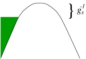
Figure 8: In the double scaling limit, the hermitian matrix model can be mapped to a system of non-interacting fermions moving through an inverse oscillator potential, one side of which has been filled up to a Fermi level at $\Delta\kappa=\kappa-\kappa_{c}\sim g_{s}^{-1}$.

Concerning the application of Liouville theory to the condensation of tachyons, there exist a few quite encouraging recent developments. Let us recall that the description of tachyon condensation requires sending the parameter $b$ to $b=i$ and evaluating the correlators for imaginary momenta $P$. We can at least find one quantity for which this procedure may be carried out easily. It is the coupling of closed strings to a decaying brane, i.e. the 1-point coupling $B$ in the theory (23) with $\Phi=0$ and $\Psi=\mu_{B}$. In fact, from the formula (45) we read off that

$$\langle\,\exp\left(iEX^{0}(z,{\bar{z}})\right)\,\rangle\ \sim\ \left(\pi\mu\right)^{iE}\,\frac{1}{\sinh\pi E}\ \ .$$

This result may be checked directly[60, 33] through perturbative computations[12, 44, 51]. Other quantities in the rolling tachyon background have a much more singular behavior at $b=i$. In fact, Barnes’ double $\Gamma$-function $\Gamma_{2}(x|b,b^{-1})$ is a well defined analytic function as long as ${\rm Re}b\neq 0$. If we send $b\rightarrow i$, on the other hand, $\Gamma_{2}$ diverges. Nevertheless, it can be shown[57] that the function $\Upsilon$ and the bulk couplings (42) possess a well defined limit. These limits, however, are no longer analytic and hence cannot be Wick rotated. It turns out that there are at least two different limiting theories. The first one occurs for real momenta (Euclidean target space) and it coincides with the interacting $c=1$ limit of unitary minimal models that was first discovered by Runkel and Watts[54]. A limiting bulk theory with imaginary momenta (Lorentzian target space) has also been constructed[57]. Future investigations will show whether this does provide an exact description of closed string rolling tachyons.

Even though Liouville theory is the only non-rational model that has been solved completely, there exist at least partial solutions for a few other non-compact backgrounds. These include the $H^{+}_{3}\cong$ SL($2,\mathbb{C}$)/SU(2) model, a non-compact relative of the group manifold SU(2) and Euclidean version of $AdS_{3}\sim$ SL(2,$\mathbb{R}$). The bulk structure constants $C$ of this theory were found several years ago by Teschner[61] and couplings $B$ of closed strings to various branes have been proposed[48, 34]. Open string couplings $C$ for non-compact branes in $H^{+}_{3}$, on the other hand, remain unknown.

Let us point out that $H_{3}^{3}$ model itself suffers from an imaginary magnetic field and hence is unphysical. But its solution represented a key step toward the construction of two rather important string backgrounds. The first concerns the description of strings in $AdS_{3}$. In a series of papers[36, 37, 38], amplitudes in this Lorentzian version of the $H^{+}_{3}$ model have been worked out and interpreted. Another interesting application arises from the coset space $H^{+}_{3}/\mathbb{R}$. This model became famous as the Euclidean 2D black hole[65]. It is a non-compact analogue of parafermions and hence a close relative of $N=2$ minimal models. Non-compact parafermions and $N=2$ minimal models have been argued to be T-dual to the Sine-Liouville (as reviewed in[30]) and the $N=2$ Liouville theory[29], respectively. References to the original literature and results on branes in these backgrounds can be found in the recent literature[52, 18].

Acknowledgement: I wish to thank the organizers of the ICMP 2003 for the opportunity to present this overview.

References

- [1] I. Affleck and A. W. W. Ludwig, Critical Theory Of Overscreened Kondo Fixed Points, Nucl. Phys. B 360 (1991) 641.
- [2] O. Aharony, S. S. Gubser, J. M. Maldacena, H. Ooguri, and Y. Oz, Large N field theories, string theory and gravity, Phys. Rept. 323 (2000) 183–386, hep-th/9905111.
- [3] A. Yu. Alekseev and V. Schomerus, D-branes in the WZW model, Phys. Rev. D60 (1999) 061901, hep-th/9812193.
- [4] A. Yu. Alekseev, A. Recknagel, and V. Schomerus, Non-commutative world-volume geometries: Branes on SU(2) and fuzzy spheres, JHEP 09 (1999) 023, hep-th/9908040.
- [5] A. Yu. Alekseev, A. Recknagel, and V. Schomerus, Brane dynamics in background fluxes and non-commutative geometry, JHEP 05 (2000) 010, hep-th/0003187.
- [6] A. Y. Alekseev, S. Fredenhagen, T. Quella, and V. Schomerus, Non-commutative gauge theory of twisted D-branes, hep-th/0205123.
- [7] S. Y. Alexandrov, V. A. Kazakov and D. Kutasov, Non-perturbative effects in matrix models and D-branes, JHEP 0309 (2003) 057, hep-th/0306177.
- [8] E. Barnes, The theory of the double gamma function, Philos. Trans. Roy. Soc. A196 (1901) 265.
- [9] A. A. Belavin, A. M. Polyakov, and A. B. Zamolodchikov, Infinite conformal symmetry in two-dimensional quantum field theory, Nucl. Phys. B241 (1984) 333–380.
- [10] M. Bianchi and A. Sagnotti, On The Systematics Of Open String Theories, Phys. Lett. B 247 (1990) 517.
- [11] L. Birke, J. Fuchs, and C. Schweigert, Symmetry breaking boundary conditions and WZW orbifolds, Adv. Theor. Math. Phys. 3 (1999) 671–726, hep-th/9905038.
- [12] C. G. . Callan, I. R. Klebanov, A. W. W. Ludwig and J. M. Maldacena, Exact solution of a boundary conformal field theory, Nucl. Phys. B 422, 417 (1994), hep-th/9402113.
- [13] J. L. Cardy, Boundary conditions, fusion rules and the Verlinde formula, Nucl. Phys. B324 (1989) 581.
- [14] C.-S. Chu and P.-M. Ho, Noncommutative open string and D-brane, Nucl. Phys. B550 (1999) 151, hep-th/9812219.
- [15] H. Dorn and H. J. Otto, Two and three point functions in Liouville theory, Nucl. Phys. B429 (1994) 375–388, hep-th/9403141.
- [16] M. R. Douglas and C. Hull, D-branes and the noncommutative torus, JHEP 02 (1998) 008, hep-th/9711165.
- [17] M. R. Douglas and N. A. Nekrasov, Noncommutative field theory, Rev. Mod. Phys. 73 (2001) 977, hep-th/0106048.
- [18] T. Eguchi and Y. Sugawara, Modular bootstrap for boundary N = 2 Liouville theory, JHEP 0401 (2004) 025, hep-th/0311141.
- [19] S. Elitzur and G. Sarkissian, D-branes on a gauged WZW model, Nucl. Phys. B625 (2002) 166–178, hep-th/0108142.
- [20] V. Fateev, A. B. Zamolodchikov and A. B. Zamolodchikov, Boundary Liouville field theory. I: Boundary state and boundary two-point function, hep-th/0001012.
- [21] G. Felder, J. Fröhlich, J. Fuchs, and C. Schweigert, The geometry of WZW branes, J. Geom. Phys. 34 (2000) 162–190, hep-th/9909030.
- [22] S. Fredenhagen and V. Schomerus, Branes on group manifolds, gluon condensates, and twisted K-theory, JHEP 0104 (2001) 007, hep-th/0012164.
- [23] S. Fredenhagen and V. Schomerus, D-branes in coset models, JHEP 02 (2002) 005, hep-th/0111189.
- [24] J. Fuchs and C. Schweigert, Symmetry breaking boundaries. I: General theory, Nucl. Phys. B 558 (1999) 419, hep-th/9902132.
- [25] M. R. Gaberdiel and T. Gannon, Boundary states for WZW models, hep-th/0202067.
- [26] K. Gawedzki, Boundary WZW, G/H, G/G and CS theories, hep-th/0108044.
- [27] M. Gutperle, M. Headrick, S. Minwalla and V. Schomerus, Space-time energy decreases under world-sheet RG flow, JHEP 0301 (2003) 073, hep-th/0211063.
- [28] M. Gutperle and A. Strominger, Timelike boundary Liouville theory, Phys. Rev. D 67 (2003) 126002, hep-th/0301038.
- [29] K. Hori and A. Kapustin, Duality of the fermionic 2d black hole and N = 2 Liouville theory as mirror symmetry, JHEP 0108 (2001) 045, hep-th/0104202.
- [30] V. Kazakov, I. K. Kostov and D. Kutasov, A matrix model for the two-dimensional black hole, Nucl. Phys. B 622 (2002) 141, hep-th/0101011.
- [31] I. R. Klebanov, String theory in two-dimensions, hep-th/9108019.
- [32] I. R. Klebanov, J. Maldacena and N. Seiberg, D-brane decay in two-dimensional string theory, JHEP 0307 (2003) 045, hep-th/0305159.
- [33] F. Larsen, A. Naqvi and S. Terashima, Rolling tachyons and decaying branes, JHEP 0302 (2003) 039, hep-th/0212248.
- [34] P. Lee, H. Ooguri and J. w. Park, Boundary states for AdS(2) branes in AdS(3), Nucl. Phys. B 632 (2002) 283, hep-th/0112188.
- [35] J. M. Maldacena, The large N limit of superconformal field theories and supergravity, Adv. Theor. Math. Phys. 2 (1998) 231 [Int. J. Theor. Phys. 38 (1999) 1113], hep-th/9711200.
- [36] J. M. Maldacena and H. Ooguri, Strings in AdS(3) and SL(2,R) WZW model. I, J. Math. Phys. 42 (2001) 2929, hep-th/0001053.
- [37] J. M. Maldacena, H. Ooguri and J. Son, Strings in AdS(3) and the SL(2,R) WZW model. II: Euclidean black hole, J. Math. Phys. 42 (2001) 2961, hep-th/0005183.
- [38] J. M. Maldacena and H. Ooguri, Strings in AdS(3) and the SL(2,R) WZW model. III: Correlation functions, Phys. Rev. D 65 (2002) 106006, hep-th/0111180.
- [39] J. Maldacena, G. W. Moore, and N. Seiberg, Geometrical interpretation of D-branes in gauged WZW models, JHEP 07 (2001) 046, hep-th/0105038.
- [40] E. J. Martinec, The annular report on non-critical string theory, hep-th/0305148.
- [41] J. McGreevy and H. Verlinde, Strings from tachyons: The c = 1 matrix reloaded, JHEP 0312 (2003) 054 hep-th/0304224.
- [42] M. Oshikawa and I. Affleck, Boundary conformal field theory approach to the critical two-dimensional Ising model with a defect line, Nucl. Phys. B495 (1997) 533–582, cond-mat/9612187.
- [43] V. B. Petkova and J. B. Zuber, Boundary conditions in charge conjugate sl(N) WZW theories, hep-th/0201239.
- [44] J. Polchinski and L. Thorlacius, Free Fermion Representation Of A Boundary Conformal Field Theory, Phys. Rev. D 50, 622 (1994), hep-th/9404008.
- [45] J. Polchinski, TASI lectures on D-branes, hep-th/9611050.
- [46] B. Ponsot and J. Teschner, Liouville bootstrap via harmonic analysis on a noncompact quantum group, hep-th/9911110.
- [47] B. Ponsot and J. Teschner, Boundary Liouville field theory: Boundary three point function, Nucl. Phys. B622 (2002) 309–327, hep-th/0110244.
- [48] B. Ponsot, V. Schomerus and J. Teschner, Branes in the Euclidean AdS(3), JHEP 0202 (2002) 016, hep-th/0112198.
- [49] G. Pradisi and A. Sagnotti, Open String Orbifolds, Phys. Lett. B 216 (1989) 59.
- [50] T. Quella and V. Schomerus, Symmetry breaking boundary states and defect lines, JHEP 06 (2002) 028, hep-th/0203161.
- [51] A. Recknagel and V. Schomerus, Boundary deformation theory and moduli spaces of D-branes, Nucl. Phys. B 545, 233 (1999), hep-th/9811237.
- [52] S. Ribault and V. Schomerus, Branes in the 2-D black hole, JHEP 0402 (2004) 019, hep-th/0310024.
- [53] I. Runkel, Boundary structure constants for the A-series Virasoro minimal models, Nucl. Phys. B549 (1999) 563, hep-th/9811178.
- [54] I. Runkel and G. M. T. Watts, A non-rational CFT with c = 1 as a limit of minimal models, JHEP 09 (2001) 006, hep-th/0107118.
- [55] V. Schomerus, D-branes and deformation quantization, MLI-13-1998-99, JHEP 06 (1999) 030, hep-th/9903205.
- [56] V. Schomerus, Lectures on branes in curved backgrounds, Class. Quant. Grav. 19 (2002) 5781, hep-th/0209241.
- [57] V. Schomerus, Rolling tachyons from Liouville theory, JHEP 0311 (2003) 043, hep-th/0306026.
- [58] N. Seiberg, Notes On Quantum Liouville Theory And Quantum Gravity, Prog. Theor. Phys. Suppl. 102 (1990) 319.
- [59] N. Seiberg and E. Witten, String theory and noncommutative geometry, JHEP 09 (1999) 032, hep-th/9908142.
- [60] A. Sen, Rolling tachyon, JHEP 0204 (2002) 048, hep-th/0203211.
- [61] J. Teschner, On structure constants and fusion rules in the SL(2,C)/SU(2) WZNW model, Nucl. Phys. B 546 (1999) 390, hep-th/9712256.
- [62] J. Teschner, Remarks on Liouville theory with boundary, hep-th/0009138.
- [63] J. Teschner, Liouville theory revisited, Class. Quant. Grav. 18 (2001) R153–R222, hep-th/0104158.
- [64] J. Teschner, A lecture on the Liouville vertex operators, hep-th/0303150.
- [65] E. Witten, On string theory and black holes, Phys. Rev. D 44 (1991) 314.
- [66] A. B. Zamolodchikov and A. B. Zamolodchikov, Structure constants and conformal bootstrap in Liouville field theory, Nucl. Phys. B477 (1996) 577–605, hep-th/9506136.
- [67] A. B. Zamolodchikov and A. B. Zamolodchikov, Liouville field theory on a pseudosphere, hep-th/0101152.