Quantum Mechanics of a Charged Particle in an Axial Magnetic Field

Abstract

We study some aspects of the quantum theory of a charged particle moving in a time-independent, uni-directional magnetic field. When the field is uniform, we make a few clarifying remarks on the use of angular momentum eigenstates and momentum eigenstates with the diamagnetism of a free electron gas as an example. When the field is non-uniform but weakly varying, we discuss both perturbative and non-perturbative methods for studying a quantum mechanical system. As an application, we derive the quantized energy levels of a charged particle in a Helmholtz coil, which go over to the usual Landau levels in the limit of a uniform field.

I Introduction

Although the quantum theory of a charged particle moving in a uni-directional constant magnetic field has been studied over many decades (for some text-book treatments, see for example magnetic ), we would like to make some clarifying remarks which we believe are useful. In studying this problem, one has to make a choice of the gauge. Different gauge choices, of course, lead to a trivial phase redefinition of the wave function. Moreover, corresponding to specific gauges, one chooses either a wave function which is an eigenstate of the momentum operator (which has continuous eigenvalues) or that of the angular momentum operator (which has discrete eigenvalues). In section II we point out that such a choice is unessential and derive an explicit relation between the two bases. This is then used in the treatement of diamagnetism of a free electron gas with angular momentum eigenstates. In section III, we study the case when the magnetic field has a weak $z$-dependence (where the $z$-axis is in the direction of the field). Then, there must be also a weak radial field and we work under conditions where it is consistent to treat this component of the field perturbatively. We find the energy eigenvalues for certain models of the $z$-dependence. These models could approximate the field between two parallel circular currents. In section IV, we discuss the form of the wave-function for large quantum numbers associated with the $z$-motion, using a non-perturbative approach in a slowly varying field. As an application, we study in section V the structure of the quantized energy levels of a charged particle in a Helmholtz coil, which are specified by two quantum numbers. The first is associated with the motion in the $(x,y)$ plane, while the second characterizes the motion in the $z$-direction. This energy spectrum may be regarded as a generalization of the Landau levels magnetic to the case of a slowly varying magnetic field. A brief conclusion is presented in section VI.

II Uniform magnetic field

We take the field to be in the $z$-direction, and to have $z$-component $B$. We take the particle’s charge and mass to be $e$ and $m$. Two gauges for the vector potential which are commonly used are

$${\bf A}=(-By/2,Bx/2,0)$$ (1)

and

$${\bf A}=(-By,0,0).$$ (2)

But the difference between these two gauges can only be trivial, since the wave-functions just differ by the phase factor

$$\omega=\exp[ieBxy/(2c\hbar)].$$ (3)

Therefore we might just as well choose (1).

For shortness, we define

$${\cal B}=eB/c$$ (4)

The Hamiltonian in gauge (1) is

$$H={1\over 2m}[(p_{x}-{\cal B}y/2)^{2}+(p_{y}+{\cal B}x/2)^{2}+p_{z}^{2}]$$

$$={1\over 2m}[p_{x}^{2}+p_{y}^{2}+p_{z}^{2}+{\cal B}^{2}(x^{2}+y^{2})/4+{\cal B}L]=H^{\prime}+p_{z}^{2}/2m,$$ (5)

where

$$p_{x}=-i\hbar{\partial\over\partial x},\leavevmode\nobreak\ \leavevmode\nobreak\ p_{y}=-i\hbar{\partial\over\partial y},\leavevmode\nobreak\ \leavevmode\nobreak\ p_{z}=-i\hbar{\partial\over\partial z},$$ (6)

$$L=xp_{y}-yp_{x}\,.$$ (7)

We define also

$$P_{x}=p_{x}+{\cal B}y/2,\leavevmode\nobreak\ \leavevmode\nobreak\ P_{y}=p_{y}-{\cal B}x/2.$$ (8)

Then the operators $P_{x},P_{y}$ and $L$ each commute with $H$ and $p_{z}$. But they don’t commute with each other:

$$[P_{x},P_{y}]=i\hbar{\cal B},\leavevmode\nobreak\ \leavevmode\nobreak\ [L,P_{x}]=i\hbar P_{y},\leavevmode\nobreak\ \leavevmode\nobreak\ [L,P_{y}]=-i\hbar P_{x}$$ (9)

We may choose the wave-function $\psi(x,y,z)$ to be an eigenfunction of $p_{z}$ with eigenvalue $\hbar k_{z}$:

$$\psi(x,y,z)=e^{ik_{z}z}\phi(x,y).$$ (10)

$$H\psi=e^{ik_{z}z}[H^{\prime}+\hbar^{2}k_{z}^{2}/(2m)]\phi,$$ (11)

and from now on we will be concerned with $H^{\prime}$ and $\phi(x,y)$.

We may choose $\phi$ to be an eigenfunction of any one of the three operators $P_{x},P_{y},L$. We discuss the two cases (i) eigenfunction of $P_{x}$ (by rotational invariance we can equally well choose it to be an eigenstates of $P_{y}$) and (ii) eigenfunction of $L$. These wave-functions may be written in a more compact form if we define a magnetic length $l$ by

$$l=\sqrt{\hbar/{\cal B}}.$$ (12)

In case (i), we have

$$\phi_{k_{x},n}(x,y)={1\over\sqrt{2\pi}}e^{ik_{x}x}e^{-ixy/2l^{2}}\xi_{n}(y),$$ (13)

where $\hbar k_{x}$ is the eigenvalue of $P_{x}$, and $\xi_{n}$ satisfies

$${\hbar^{2}\over 2m}\left[-{\partial^{2}\over\partial y^{2}}+\{(y/l^{2})-k_{x}\}^{2}\right]\xi_{n}(y)=E^{\prime}\xi_{n}(y),$$ (14)

$E^{\prime}$ being the eigenvalue of $H^{\prime}$. This equation describes a simple harmonic oscillator whose equilibrium point is shifted, and the eigenfunctions have the form

$$\xi_{n}(y)=l^{-1/2}u_{n}[(y-\eta)/l],$$ (15)

where $n$ is a positive integer,

$$\eta=l^{2}k_{x}\,,\leavevmode\nobreak\ \leavevmode\nobreak\ E^{\prime}={\hbar{\cal B}\over m}(n+{1\over 2})$$ (16)

and $u_{n}(w)$ is the real, normalized solution of

$$\left[-{\partial^{2}\over\partial w^{2}}+w^{2}\right]u_{n}(w)=(2n+1)u_{n}(w).$$ (17)

Next we take the case (ii), where we use energy eigenfunctions which are also eigenfunctions of angular momentum $L$ with eigenvalue $\hbar M$. We denote these normalized wave-functions by

$$\zeta_{n,M}(x,y).$$ (18)

Eigenfunctions of type (i), in equation (13), are non-normalizable and have a continuous degeneracy, whereas those of type (ii) in (18) are normalized and have a discrete degeneracy. Nevertheless, it should be possible to express each type in terms of the other. To this end, we consider a superposition of the form

$$\chi_{n,f}=\int dk_{x}f(k_{x})\phi_{k_{x},n}(x,y)$$ (19)

where $f$ is some function to be determined and

$$\int dxdy\chi^{*}_{n^{\prime},f}\chi_{n,f}=\delta_{nn^{\prime}}\int dk_{x}|f(k_{x})|^{2}.$$ (20)

In order to make (19) an eigenstate of $L$, we require

$$\hbar M\chi_{n,f}=L\chi_{n,f}$$

$$=-i\hbar(2\pi l)^{-1/2}\int dk_{x}f(k_{x})\left(x{\partial\over\partial y}-y{\partial\over\partial x}\right)$$

$$\times\exp[ik_{x}x-ixy/2l^{2}]u_{n}[(y/l)-lk_{x}].$$ (21)

We convert $x$ and $x^{2}$ into derivatives of $e^{ik_{x}x}$ and integrate by parts to put these derivatives onto $f$ and $u$. In this way, we find that equation (21) is satisfied provided $f$ obeys

$$-{1\over l^{2}}{d^{2}f\over dk_{x}^{2}}+l^{2}k_{x}^{2}f=[2(n-M)+1]f.$$ (22)

This equation is consistent, and its normalised solution is just

$$f(k_{x})=l^{1/2}u_{n-M}[lk_{x}].$$ (23)

Thus, finally, the required eigenfunction of $L$ is determined to be

$$\zeta_{n,M}(x,y)=l^{1/2}\int dk_{x}u_{n-M}(lk_{x})\phi_{k_{x},n}(x,y).$$ (24)

Using the ortho-normality of the $u_{n}$ coefficients in (24), we can invert this equation to find the momentum eigenfunctions in terms of the angular momentum eigenfunctions:

$$\phi_{k_{x},n}(x,y)=l^{1/2}\sum_{M=-\infty}^{n}u_{n-M}(lk_{x})\zeta_{n,M}(x,y).$$ (25)

The text-book treatment (see for example diamagnetism ) of the diamagnetism of a free electron gas is usually formulated in terms of the eigenfunctions of momentum (13). The sample is considered to have a finite size with dimensions $S_{x},S_{y}$ in the $x$- and $y$-directions, in which case states contribute only for

$$|\eta|<S_{y}.$$ (26)

So the number of states with a given energy and value of $k_{z}$ is

$${{\cal B}S_{x}S_{y}\over 2\pi\hbar}={S_{x}S_{y}\over 2\pi l^{2}}$$ (27)

It ought to be possible to carry out the analysis using the angular momentum eigen-functions (18). In that case, it is natural to consider a cylindrical sample, axis along the $z$ axis, with radius $R$. The asymptotic form of the wave function (18), for large $\rho$, is proportional to

$$e^{iM\phi}\rho^{2n-M}\exp(-\rho^{2}/4l^{2}),$$ (28)

and this has its maximum at

$$\rho_{max}=\sqrt{2(2n-M)}\,\,l.$$ (29)

Thus we expect states to contribute for

$$2n-M<{R^{2}\over 2l^{2}}.$$ (30)

Then, for given $n$, the range of $M$ is

$$2n-{R^{2}\over 2l^{2}}\leq M\leq n,$$ (31)

so that the number of possible values of $M$ is

$${R^{2}\over 2l^{2}}-n.$$ (32)

The relevant values of $n$ are of order $(mkTl^{2}/\hbar^{2})$ which is small compared to $(R^{2}/l^{2})$ for typical values of $B$, $R$ and $T$ (temperature). Thus (32) gives a factor

$${\pi R^{2}\over 2\pi l^{2}}$$ (33)

which is proportional to the area just as in (27).

III Weakly varying magnetic field

We now allow the magnetic field to vary slowly with $z$, but we restrict ourselves to motion near the $z$-axis. Along the axis, we use an expansion

$$B_{z}(z)=B_{0}[1+b_{1}(z/a)^{2}+b_{2}(z/a)^{4}+...]$$ (34)

where $a$ is a characteristic length.

A realistic case would be a pair of two similar current loops, each perpendicular to the common $z$-axis and of radius $a$, separated by a distance $2d$. This system, known as the Helmholtz coil, is shown in Fig. 1.

Figure 1: Schematic illustration of a Helmholtz coil.

Near the origin the field has an expansion of the above form, where $B_{0}$ is determined by the current carried by the loops and (in terms of $r=(d/a)^{2}$)

$$b_{1}={3(4r-1)\over 2(r+1)^{2}},\leavevmode\nobreak\ \leavevmode\nobreak\ \leavevmode\nobreak\ b_{2}={15(1-12r+8r^{2})\over 8(r+1)^{4}}.$$ (35)

Off the axis, the magnetic field must have some radial component. Up to second order (that is the $b_{1}$ term), we take the vector potential to be

$${\bf A}={1\over 2}B_{0}[1+b_{1}(z^{2}-\rho^{2}/4)/a^{2}](-y,x,0).$$ (36)

This form follows by rotational symmetry (if the field is generated by currents in circles about the axis), together with the gauge choice $\mbox{\boldmath$\nabla$}\cdot{\bf A}$$=0$ and Maxwell’s equation $\nabla^{2}{\bf A}=0$.

As the leading approximation, we keep just the $b_{1}z^{2}$ term in (34) (we shall see that the $\rho^{2}$ term is effectively smaller). We seek an energy eigenfunction of the Hamiltonian (5), with ${\cal B}$ now $z$-dependent, of the form

$$W(z)\Phi(x,y).$$ (37)

Then the equation for $W$ is (we now define $l$ to be $\sqrt{\hbar/{\cal B}_{0}}$)

$$-{d^{2}W\over dz^{2}}+(2n+1){b_{1}z^{2}\over a^{2}l^{2}}W={2m\Delta E\over\hbar^{2}}W,$$ (38)

where the second term on the left comes from $E^{\prime}$ in (14) when $B$ is $z$-dependent. This is just the equation for a simple harmonic oscillator and, for $k_{z}=0$, the energy associated with the $z$ motion is

$$\Delta E={\hbar^{2}\over mal}\sqrt{b_{1}(2n+1)}(N+{1\over 2}).$$ (39)

We can now treat the $z^{4}$ term in (34) and the $\rho^{2}$ term in (36) as perturbations. These terms are of the same order. This is because the transverse size of the wave-function is of order $l$ whereas the longitudinal size is of order $\sqrt{la}$. Note that, as an example, for a magnetic flux density of 1 tesla, $l=2.5\times 10^{-8}m$.

Treating the $z^{4}$ term by perturbation theory, we find an additional energy

$$\Delta E^{\prime}={3\hbar^{2}\over 4ma^{2}}{b_{2}\over b_{1}(2n+1)}(1+2N+2N^{2}).$$ (40)

Note that this is independent of $B$ and usually very small if $a$ is macroscopic. However, for large values of $N$, the contributions from the $b_{2}$ term and higher terms in (34) may be significant.

We also treat by perturbation theory the $\rho^{2}$ term in (36). To this end we require, inserting the $\rho^{2}$ term in (36) into the Hamiltonian (5),

$$\Delta E^{\prime\prime}=-{\hbar b_{1}\over 16ma^{2}l^{2}}\int dxdy\phi^{*}_{n,M}(2L\rho^{2}+\hbar\rho^{4}/l^{2})\phi_{n,M}.$$ (41)

These expectation values can be worked out using:

$$\int dxdy\psi^{*}\rho^{2}\psi=(2n-M+1)l^{2},$$ (42)

$$\int dxdy\psi^{*}\rho^{4}\psi=[(2n-M+1)^{2}+2n(n-M)+2n-M+1]l^{4}.$$ (43)

As a result, we have

$$\Delta E^{\prime\prime}=-{\hbar^{2}b_{1}\over 16ma^{2}}[6n(n+1)-M(M+1)+2(1-nM)].$$ (44)

This is independent of $B$ and, in general, is much smaller than (40) for large values of $N$.

IV Non-perturbative approach to a slowly varying field

We have seen that when the quantum number associated with the $z$-motion is large, $N>>n$, the dependence of $B_{z}$ upon $\rho$ may be neglected in first approximation. In this case, the vector potential may be written as:

$${\bf A}={1\over 2}B_{z}(z)(-y,x,0)\,.$$ (45)

This leads to the Schrödinger equation:

$${\partial^{2}\psi\over\partial\rho^{2}}+{1\over\rho}{\partial\psi\over\partial\rho}-\bigg{(}{M^{2}\over\rho^{2}}+{eB_{z}M\over\hbar c}+{e^{2}B_{z}^{2}\over 4\hbar^{2}c^{2}}\rho^{2}\bigg{)}\psi+{\partial^{2}\psi\over\partial z^{2}}=-{2m\over\hbar^{2}}E\psi\,,$$ (46)

where we have taken the energy eigenfunction to be also an eigenfunction of the angular momentum $L_{z}$ with eigenvalue $\hbar M$. Let us consider a solution of the form:

$$\psi(\phi,\rho,z)=F(\phi,\rho,z)f(z)$$ (47)

and assume, since the field is slowly varying, that:

$$\bigg{|}{\partial F\over\partial z}\bigg{|}<<\bigg{|}{\partial F\over\partial\rho}\bigg{|}\,.$$ (48)

Then, the Schrödinger equation (46) takes the form:

$${1\over F}\bigg{[}{\partial^{2}F\over\partial\rho^{2}}+{1\over\rho}{\partial F\over\partial\rho}\bigg{]}-{M^{2}\over\rho^{2}}-{eB_{z}M\over\hbar c}-{e^{2}B_{z}^{2}\over 4\hbar^{2}c^{2}}\rho^{2}=-\bigg{[}{1\over f}{d^{2}f\over dz^{2}}+{2m\over\hbar^{2}}E\bigg{]}\,.$$ (49)

The right hand side of (49) depends on $z$ only, so that we have:

$${d^{2}f\over dz^{2}}+{2m\over\hbar^{2}}Ef={2m\over\hbar^{2}}E^{\prime}(z)f$$ (50)

and

$${\partial^{2}F\over\partial\rho^{2}}+{1\over\rho}{\partial F\over\partial\rho}-\bigg{(}{M^{2}\over\rho^{2}}+{eB_{z}M\over\hbar c}+{e^{2}B_{z}^{2}\rho^{2}\over 4\hbar^{2}c^{2}}\bigg{)}F=-{2m\over\hbar^{2}}E^{\prime}(z)F\,.$$ (51)

But we know how to solve (51), in which $z$ is just a parameter. Comparing with (16), we see that:

$$E^{\prime}(z)={e\hbar\over mc}(n+{1\over 2})B_{z}(z)\,.$$ (52)

Thus, (50) may be written as:

$${d^{2}f\over dz^{2}}+{2m\over\hbar^{2}}\bigg{[}E-{e\hbar(2n+1)\over 2mc}B_{z}(z)\bigg{]}f=0\,,$$ (53)

which is just an ordinary differential equation.

We can now check the assumption (48). The solutions of (51) have the form (18), namely:

$$F(\phi,\rho,z)=\zeta_{n,M}(\phi,\sqrt{{eB_{z}\over 2\hbar c}}\,\rho)\,.$$ (54)

Hence, the condition (48) requires that:

$${\rho\over B_{z}}{dB_{z}\over dz}<<1\,.$$ (55)

Although this cannot be satisfied for all $\rho$, we note that the solution (54) contains the factor:

$$\exp[-{eB_{z}\over 4\hbar c}\rho^{2}]\,,$$ (56)

so that typical values of $\rho$ are of order $\sqrt{\hbar c/eB_{z}}$. Thus, we expect (55) to be valid for:

$$\sqrt{{\hbar c\over e}}{1\over B_{z}^{3/2}}{dB_{z}\over dz}<<1\,.$$ (57)

This can be satisfied provided we take $B_{z}$ to be varying slowly enough. For instance, if $B_{z}(z)$ has the form (34) with $|z|$ of order $a$, then the left hand side of (57) is of order $l/a$, which is very small for typical values of $B_{0}$ and $a$.

V Quantized energy levels in a Helmholtz coil

A simple example of a magnetic mirror is provided by the pair of current loops shown in Fig. 1. Then, as can be seen from equations (34) and (35) for $2d>a$, the magnetic field can increase enough in the region near the current loops, so that a charged particle may eventually be reflected out of this region towards the center of the coil. The classical restoring force which may confine the particle along the $z$-axis is provided by the $\rho$-component of the magnetic field:

$${\bf B}(z)=-{1\over 2}\rho{\partial B_{z}\over\partial z}\hat{\mbox{\boldmath$\rho$}}+B_{z}\hat{{\bf z}}\,.$$ (58)

which can be derived from (45) using ${\bf B}=\mbox{\boldmath$\nabla$}\times{\bf A}$.

In this section, we will discuss the quantized energy levels of a charged particle in a Helmholtz coil. To this end, we will analyse the basic equation (53), where

$$B_{z}(z)={1\over 2}B_{0}(d^{2}+a^{2})^{3/2}\bigg{\{}{1\over[(z+d)^{2}+a^{2}]^{3/2}}+{1\over[(z-d)^{2}+a^{2}]^{3/2}}\bigg{\}}\,.$$ (59)

The general behavior of this field, for $2d>a$, is shown in Fig. 2.

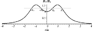
Figure 2: Pattern of the field $B_{z}(z)$ in a Helmholtz coil. Circles indicate the classical turning points.

Since (53) was derived under the assumption that $N>>1$, our analysis will be more appropriate in the semiclassical regime. This may be studied conveniently in the WKB approximation, which is particularly useful since we are dealing with a slowly varying potential:

$$V(z)={e\hbar\over 2mc}(2n+1)B_{z}(z)\,.$$ (60)

One of the most interesting results arising from the WKB method is a semiclassical estimate for the quantized energy levels in a potential. Matching the WKB wave function at each of the classical turning points, which are determined by the relation $E=V(z)$, leads to the Bohr-Sommerfeld quantization condition:

$$\int_{-Z_{+}}^{Z_{+}}\sqrt{2m[E-V(z)]}dz=(N+{1\over 2})\pi\hbar\,,$$ (61)

where the classical turning points for bound motion, $\pm Z_{+}$, are situated inside the well as shown in Fig. 2. (We neglect, in first approximation, the very small probability of tunneling through the potential barrier.)

In general, equation (61) is rather complicated and can only be solved numerically. However, when $d/a$ is somewhat larger than $1/2$, it may be solved in closed form, since in this case $z/a$ will be effectively of order $1/2$ or smaller. Then, we can expand the potential $V(z)$ [see (59) and (60)] up to terms which are of quartic order in $z/a$, as shown in equations (34) and (35). In this approximation, the quantization condition (61) may be written in the form:

$$\int_{-Z_{+}}^{Z_{+}}\sqrt{{\cal E}-1-b_{1}\big{(}{z\over a}\big{)}^{2}-b_{2}\big{(}{z\over a}\big{)}^{4}}dz=\pi\sqrt{{c\hbar\over(2n+1)eB_{0}}}(N+{1\over 2})\,,$$ (62)

where the dimensionless parameter ${\cal E}$ is defined by:

$${\cal E}={2mc\over(2n+1)e\hbar B_{0}}E\,.$$ (63)

We can now determine explicity the positions of the classical turning points, which are given by:

$$Z_{\pm}=a\bigg{[}{-b_{1}\pm\sqrt{b_{1}^{2}+4b_{2}({\cal E}-1)}\over 2b_{2}}\bigg{]}^{1/2}\,,$$ (64)

where $\pm Z_{-}$ are the turning points for unbound motion, which are situated outside the well as shown in Fig. 2. Then, the integral appearing in (62) can be evaluated in closed form in terms of the complete elliptic integrals of the first (${\bf F}$) and second (${\bf E}$) kind tables , with the result:

$${2\sqrt{-b_{2}}\over 3a^{2}}Z_{-}\bigg{[}\big{(}Z_{+}^{2}-Z_{-}^{2}\big{)}{\bf F}\bigg{(}{Z_{+}\over Z_{-}}\bigg{)}+\big{(}Z_{+}^{2}+Z_{-}^{2}\big{)}{\bf E}\bigg{(}{Z_{+}\over Z_{-}}\bigg{)}\bigg{]}=\pi\sqrt{{c\hbar\over(2n+1)eB_{0}}}(N+{1\over 2})\,.$$ (65)

This is a transcendental equation which determines implicitly the energy in terms of the quantum number $N$. The energies of the bound states have an upper bound $E^{max}$ which corresponds to the maximum value of the potential. At this energy, $Z_{+}=Z_{-}$, so that using (63) and (64) we obtain:

$$E^{max}_{n}={e\hbar B_{0}\over 2mc}(2n+1)\bigg{(}1-{b_{1}^{2}\over 4b_{2}}\bigg{)}\,.$$ (66)

When $Z_{+}=Z_{-}$, the equation (65) simplifies considerably and fixes the maximum value of the quantum number $N$, which is given by the relation:

$$N_{max}+{1\over 2}={\sqrt{2(2n+1)}\over 3\pi}{b_{1}^{3/2}\over|b_{2}|}{a\over l}\,,$$ (67)

where $l=\sqrt{c\hbar/eB_{0}}$ is the magnetic length. Hence, $N_{max}$ is in general a very large number, which is in acordance with our previous assumption.

A more explicit relation giving $E$ as a function of $N$ can be obtained by solving numerically the equation (65). As an example, the numerical solution for $n=0$ and $d/a=3/5$ is shown in Fig. 3. Here, the numerical values of ${\cal E}^{max}=1.028$ and $N_{max}=1.12\times 10^{6}$ are in good agreement with the corresponding results obtained from the closed form expressions (66) and (67). One can see that the numerical solution can be fitted reasonably well, for large quantum numbers, by a simple phenomenological form like $N^{5/6}$.

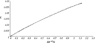
Figure 3: Numerical solution (crossed) of Eq. (65) for the energy spectrum and plot (solid) of the form $N^{5/6}$ for large $N$.

Finally, we note from (34) and (35) that for $d/a=1/2$, $b_{1}=0$ and $b_{2}=-144/125$. Then, the system of the two current loops provides a practically uniform field in the central region of the Helmholtz coil. In this case, (66) reduces to the well known expression for the Landau levels which occur in a constant field. Therefore, one may regard the quantized energies described by (65) and (66), as an extension of the Landau levels to the case of a slowly varying magnetic field.

VI Conclusion

In this paper, we have discussed several aspects concerning the quantum behavior of a charged particle in a static magnetic field. We have treated the issue of the relation between the choice of gauge and the choice of the diagonal operators which commute with the Hamiltonian of the system. We have also developed some approaches which may be useful for physical applications in a slowly varying magnetic field. These methods have been applied to study the quantized energy levels of a charged particle in a weakly varying field. Such a field may be present, for example, in a magnetic mirror like the Helmholtz coil. We have shown that this energy spectrum represents an interesting extension of the well known Landau levels which occur in an uniform magnetic field.

This work was supported in part by US DOE Grant number DE-FG 02-91ER40685, by CAPES, CNPq and FAPESP, Brazil.

Bibliography

1. L. D. Landau and E. M. Lifshitz, Quantum Mechanics: The Non-Relativistic Theory, Butterworth-Heinemann, 1981; L. E. Ballentine, Quantum Mechanics, Prentice Hall, 1990; S. Gasiorowicz, Quantum Physics (2nd edition), Wiley, 1996; E. Merzbacher, Quantum Mechanics (3rd edition), Wiley, 1998; J. Schwinger, Quantum Mechanics, Springer, 2001.
2. R. E. Peierls, Quantum Theory of Solids, Oxford University Press, 2001.
3. I. S. Gradshteyn and M. Ryzhik, Tables of Integral Series and Products, Academic Press, New York, 1980.