Particle Production in Tachyon Condensation

Abstract

We study particle production in the tachyon condensation process as described by different effective actions for the tachyon. By making use of invariant operators, we are able to obtain exact results for the density of produced particles, which is shown to depend strongly on the specific action. In particular, the rate of particle production remains finite only for one of the actions considered, hence confirming results previously appeared in the literature.

1 Introduction

One of the most intriguing features of String Theory is the tachyon condensation process and its possible description in terms of a tachyon effective theory. Finding an effective action for the tachyon field is a difficult task. Nevertheless, in certain situations (like the decay of non-BPS D-branes) some aspects of the string dynamics can be described by an effective field theory action involving only the tachyon and massless modes (see for example Refs. [1, 2]).

The form of the effective action for the tachyon depends on the choice of the region in field space where it can be valid. One such a region corresponds to the neighbourhood of the perturbative string vacuum (in which the tachyon $T=0$) where one can reconstruct the tachyon effective action from string $S$-matrix. In this case, we expect the effective action to be of the form

$$S=-\int\mbox{{\rm d}}t\,\mbox{{\rm d}}^{p}x\,\left({1\over 2}\,\eta^{\mu\nu}\,\partial_{\mu}T\,\partial_{\nu}T-{\mu^{2}\over 2}\,T^{2}+g\,T^{4}+\ldots\right)\ .$$ (1.1)

where $\eta_{\mu\nu}$ is the Minkowski metric (Greek indices run from $0$ to $p$), $\mu$ and $g$ are constants and the dots represent higher order terms.

A second possibility is trying to reconstruct the effective action near some exact conformal points. One such a conformal point is a time-dependent background that represents an exact boundary conformal field theory [4, 5, 6, 7],

$$T=f_{0}\,e^{\mu\,x^{0}}+{\bar{f}}_{0}\,e^{-\mu\,x^{0}}\ .$$ (1.2)

A special case is then the “rolling tachyon” background

$$T=f_{0}\,e^{\mu\,x^{0}}\ ,$$ (1.3)

where $\mu^{2}=1$ or $1/2$ in the bosonic and supersymmetric case respectively, which would be described by the homogeneous Lagrangian [8]

$$L=-\frac{1}{1+\frac{T^{2}}{2}}\,\sqrt{1+\frac{T^{2}}{2}-\left(\partial_{0}T\right)^{2}}\ .$$ (1.4)

If the above admits a straightforward covariant generalization, one obtains

$$S=-\int\mbox{{\rm d}}t\,\mbox{{\rm d}}^{p}x\,{1\over 1+{T^{2}\over 2}}\,\sqrt{1+{T^{2}\over 2}+\eta^{\mu\nu}\,\partial_{\mu}T\,\partial_{\nu}T}\ ,$$ (1.5)

which has just the form of a “DBI” (Dirac-Born-Infeld) action

$$S=-\int\mbox{{\rm d}}t\,\mbox{{\rm d}}^{p}x\,V(\tilde{T})\,\sqrt{1+\eta^{\mu\nu}\,\partial_{\mu}\tilde{T}\,\partial_{\nu}\tilde{T}}\ ,$$ (1.6)

where $\tilde{T}=\sqrt{2}\,\sinh\left(T/\sqrt{2}\right)$ and the potential is given by

$$V(\tilde{T})=\left(\cosh\frac{\tilde{T}}{\sqrt{2}}\right)^{-1}\ .$$ (1.7)

Even if the rolling tachyon (1.3) is an exact solution of the equation of motion that arises from the action (1.5), it is not completely clear whether such an action should be used for the description of field theory space around the perturbative vacuum $T=0$. In particular, in Refs. [9, 10, 11], the stability of the the classical time-dependent solution of Eq. (1.5) was analyzed, showing that fluctuations become large in a very short time interval and hence they might significantly change the classical evolution. One can also interpret the huge growth of fluctuations as the creation of a large number of fluctuation modes in the time-dependent background of the classical solution [12]. We can then expect that at some time near the beginning of the tachyon condensation the density of the number of particles created reaches the string density and the linearized approximation, in which fluctuations are assumed small, breaks down.

Finally, one can also consider as a starting point a tachyon effective action of the form

$$S=-\int\mbox{{\rm d}}t\,\mbox{{\rm d}}^{p}x\,\frac{1}{1+T}\sqrt{1+T+\frac{\eta^{\mu\nu}\,\partial_{\mu}T\,\partial_{\nu}T}{T}}\ ,$$ (1.8)

which arises when one considers the tachyon of a D-brane in bosonic String Theory and was derived in Ref. [13] following the proposal of Ref. [8].

We will analyze the production of particles for the three actions reviewed above by making use of Lewis’ invariant operators [14]. This technique yields exact results and will allow us to go beyond the usual linear approximation in all the cases under consideration. Our analysis follows the same line as that of Ref. [15]. In particular, we shall restrict our study of particle production to the fluctuation modes with initial momentum $k^{2}>\mu^{2}$ at infinite past. Modes with $k^{2}<\mu^{2}$ exponentially grow even at the beginning of the tachyon condensation and this may significantly change the classical evolution. The analysis of these modes is a challenging task beyond the scope of this paper and even for the modes with a positive frequency $\Omega_{k}^{2}=k^{2}-\mu^{2}$ at far past we will get some interesting results.

2 Particle Production

The fluctuations of the tachyon field obtained by using the effective Lagrangians in Eqs. (1.1), (1.5) and (1.8) may be described by the Hamiltonian of an harmonic oscillator with time dependent frequency (as shown in Ref. [15]). The formalism of Lewis’ invariant operators [14] will then provide us with the exact expressions for the number of particles produced by the time-dependence of the frequency.

2.1 DBI action

Figure 1: Particle density for the linearized approximation (dashed line) and for the exact solution (solid line) for the DBI action.

Starting with the action given in Eq. (1.5), one can show that the fluctuations of the tachyon field are governed by the Hamiltonian for an harmonic oscillator with a time dependent frequency [15]

$$\Omega^{2}_{k}(t)={k^{2}\over 1+e^{\sqrt{2}\,t}}+m^{2}\ ,\ \ \ \ m^{2}=-{1\over 2}\ .$$ (2.1)

The expression for the number of created particles is then

$$N_{k}(t)={1\over{4\,\Omega_{k}}}\,\left(\dot{\rho}^{2}+\Omega_{k}^{2}\,\rho^{2}+{1\over\rho^{2}}\right)-{1\over 2}\ .$$ (2.2)

The auxiliary function $\rho(t)$ is given by

$$\rho(t)=\sqrt{\frac{x_{1}^{2}(t)+x_{2}^{2}(t)}{\omega_{0k}}}$$ (2.3)

where $\omega_{0k}\equiv\lim_{t\rightarrow-\infty}\Omega_{k}(t)=k^{2}-1/2$, and $x_{1}(t)$ and $x_{2}(t)$ are independent solutions of the homogeneous equation

$$\ddot{x}(t)+\Omega_{k}^{2}(t)\,x(t)=0\ .$$ (2.4)

For the frequency in Eq. (2.1) they are given by

$$x_{1}(t)={1\over 2}\,\left(y_{1}(t)+y_{2}(t)\right)$$

(2.5)

$$x_{2}(t)={1\over 2i}\,\left(y_{1}(t)-y_{2}(t)\right)\ ,$$

where

$$y_{1}(t)=e^{\displaystyle{i\,\omega_{0k}\,t}}\,_{2}F_{1}\left(-{1\over 2}+{i\over\sqrt{2}}\,\omega_{0k},{1\over 2}+{i\over\sqrt{2}}\,\omega_{0k};1+i\,\sqrt{2}\,\omega_{0k};-e^{\sqrt{2}\,t}\right)$$

(2.6)

$$y_{2}(t)=e^{\displaystyle{-i\,\omega_{0k}\,t}}\,_{2}F_{1}\left(-{1\over 2}-{i\over\sqrt{2}}\,\omega_{0k},{1\over 2}-{i\over\sqrt{2}}\,\omega_{0k};1-i\,\sqrt{2}\,\omega_{0k};-e^{\sqrt{2}\,t}\right)\ ,$$

and the $F$’s are hypergeometric functions [16]. One can see from Fig. 1 that the number of produced particles diverges for a finite $t$ for $k\gg 1$ as in Ref. [15], but this effect seems to be due to the $\Omega_{k}(t)$ becoming imaginary and not to happen as $\Omega_{k}(t)\gg 1$. In any case, the production obtained by the exact method is significantly smaller than the result obtained using a linear approximation and seems to diverge at a later time. This allows for the possibility that, when backreaction effects are included, the tachyon condensation process might be correctly described by this effective action.

2.2 Bosonic Action

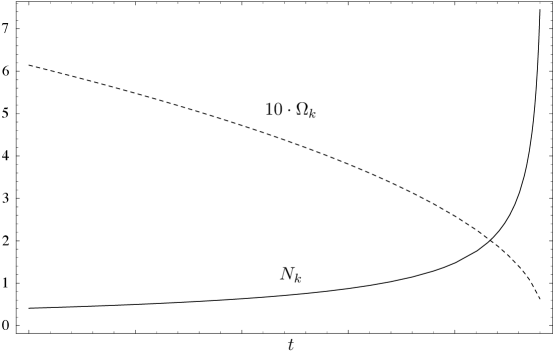
Figure 2: Particle density $N_{k}(t)$ (solid line) and frequency $10\,\Omega_{k}(t)$ (dashed line) for the Bosonic Action.

In this section we will compute the particle production on D-branes in bosonic String Theory assuming a tachyon effective action of the form given in Eq. (1.8).

In the present case the time dependent frequency is given by

$$\Omega^{2}_{k}(t)=\left(1-e^{t}\right)\,k^{2}-\frac{1}{4}\equiv\omega_{0k}^{2}-\lambda\,e^{t}\ ,$$ (2.7)

where $\omega_{0k}^{2}=k^{2}-1/4$ and $\lambda=k^{2}$. The expression for the number of produced particles is the same as in Eq. (2.2), where $x(t)$ again solves the homogenous equation of the harmonic oscillator with frequency $\Omega_{k}$. We then have

$$x_{1}(t)={1\over 2}\,\left[I_{2\,i\,\omega_{0k}}\left(2\,k\,e^{t/2}\right)\,\Gamma\left(1+2\,i\,\omega_{0k}\right)+I_{-2\,i\,\omega_{0k}}\left(2\,k\,e^{t/2}\right)\,\Gamma\left(1-2\,i\,\omega_{0k}\right)\right]$$

(2.8)

$$x_{2}(t)={1\over 2\,i}\,\left[I_{2\,i\,\omega_{0k}}\left(2\,k\,e^{t/2}\right)\,\Gamma\left(1+2\,i\,\omega_{0k}\right)-I_{-2\,i\,\omega_{0k}}\left(2\,k\,e^{t/2}\right)\,\Gamma\left(1-2\,i\,\omega_{0k}\right)\right]\ ,$$

where the $I$’s are Bessel functions [16]. Particle production becomes relevant shortly after the condensation process has begun, due to the fact that $\Omega_{k}(t)$ becomes imaginary, as is shown in Fig. 2 (in which $\Omega_{k}$ is multiplied by a factor of 10 for convenience).

2.3 Perturbative Effective Action

Figure 3: Particle density $N_{k}(t)$ (solid line) and frequency variation $\dot{\Omega}_{k}(t)/\Omega^{2}_{k}(t)$ (dashed line) for the Bosonic Action.

On using the action in Eq. (1.1), one obtains the Hamiltonian of an harmonic oscillator with time dependent frequency

$$\Omega^{2}_{k}(t)=6\,g\,e^{2\,\mu\,t}+k^{2}-\mu^{2}\equiv\lambda\,e^{2\,\mu\,t}+\omega_{0k}^{2}\ ,$$ (2.9)

where $\omega_{0k}^{2}=k^{2}-\mu^{2}$ and $\lambda=6\,g$. The expression for the number of produced particles is again the same as that in Eq. (2.2), with

$$x_{1}(t)={1\over 2}\,\left[J_{i\,{\omega_{0k}\over\mu}}\,\left(\sqrt{6\,g\over\mu^{2}}\,e^{\mu\,t}\right)\,\Gamma\left(1+i\,{\omega_{0k}\over\mu}\right)+J_{-i\,{\omega_{0k}\over\mu}}\left(\sqrt{6\,g\over\mu^{2}}\,e^{\mu\,t}\right)\,\Gamma\left(1-i\,{\omega_{0k}\over\mu}\right)\right]$$

(2.10)

$$x_{2}(t)={1\over 2\,i}\,\left[J_{i\,{\omega_{0k}\over\mu}}\left(\sqrt{6\,g\over\mu^{2}}\,e^{\mu\,t}\right)\,\Gamma\left(1+i\,{\omega_{0k}\over\mu}\right)-J_{-i\,{\omega_{0k}\over\mu}}\left(\sqrt{6\,g\over\mu^{2}}\,e^{\mu\,t}\right)\,\Gamma\left(1-i\,{\omega_{0k}\over\mu}\right)\right]\ ,$$

where the $J$’s are Bessel functions and $\Gamma$ the Gamma function [16].

We can now restrict the analysys to the bosonic case ($\mu^{2}=1$), since for the supersymetric case ($\mu^{2}=1/2$) the situation is exactly the same. The number of produced particles is plotted in Fig. 3. One will note that the density of the produced particles reaches a maximum as the variation of $\Omega_{k}(t)$ varies more rapidly and then settles down. This behavior strongly suggests that the corresponding action (1.1) might then be suitable for describing the condensation process up to the time when the linear approximation breaks down (that is when $\mu^{2}\,T^{2}\simeq g\,T^{4}$).

3 Conclusions

We have computed the density of particles produced in the early stages of the tachyon condensation. The use of invariant operators allows us to obtain exact results and to show that the production rate strongly depends on the form of the action. The DBI action (1.5) and the Bosonic Action (1.8) produce divergent densities in the early stages of the tachyon condensation, whereas the Perturbative Effective Action (1.1) seems to yield a regular behavior when the linearized approximation is satisfied. This suggests that such an action should be regarded as the most suitable candidate to describe the process of tachyon condensation. On the other hand one should note that backreaction effects have been neglected in our approach. Any conclusions therefore need to be confirmed by an analysis that takes into account the backreaction, and our results must be considered as preliminary until a more thorough (and very likely numerical) analysis is performed. This is left for future research beyond the scope of this paper.

References

- [1] N. D. Lambert and I. Sachs, Phys. Rev. D 67 (2003) 026005 [hep-th/0208217].
- [2] N. D. Lambert and I. Sachs, JHEP 0106 (2001) 060 [hep-th/0104218].
- [3] A. A. Tseytlin, J. Math. Phys. 42 (2001) 2854 [hep-th/0011033].
- [4] A. Sen, Mod. Phys. Lett. A 17 (2002) 1797 [hep-th/0204143].
- [5] A. Sen, JHEP 0207 (2002) 065 [hep-th/0203265].
- [6] A. Sen, JHEP 0204 (2002) 048 [hep-th/0203211].
- [7] M. Gutperle and A. Strominger, Phys. Rev. D 67 (2003) 126002 [hep-th/0301038].
- [8] D. Kutasov and V. Niarchos, “Tachyon effective actions in open string theory”, hep-th/0304045.
- [9] M. Berkooz, B. Craps, D. Kutasov and G. Rajesh, JHEP 0303 (2003) 031 [hep-th/0212215].
- [10] G. N. Felder, L. Kofman and A. Starobinsky, JHEP 0209 (2002) 026 [hep-th/0208019].
- [11] A. V. Frolov, L. Kofman and A. A. Starobinsky, Phys. Lett. B 545 (2002) 8 [hep-th/0204187].
- [12] J. Kluson, “Particle production on half S-brane”, hep-th/0306002.
- [13] J. Kluson, “Note on D-brane effective action in the linear dilaton background”, hep-th/0310076.
- [14] H.R. Lewis, J. Math. Phys. 9 (1968) 1976; H.R. Lewis and W.B. Riesenfeld, J. Math. Phys. 10 (1969) 1458.
- [15] J. Kluson, JHEP 0401 (2004) 019 [hep-th/0312086].
- [16] M. Abramowitz and I. Stegun, Handbook of mathematical functions with formulas, graphs, and mathematical table, Dover Publishing (1965).