Through the Looking Glass:

AdS-FT with time dependent boundary conditions and black hole formation

Keith Copsey

Department of Physics, UCSB, Santa Barbara, CA 93106

keith@physics.ucsb.edu

I solve for the behavior of scalars in Lorentzian AdS with time dependent boundary conditions, focusing in particular on the dilaton. This corresponds, via the AdS-CFT correspondence, to considering a gauge theory with a time dependent coupling. Changes which keep the gauge coupling nonzero result in finite but physically interesting states in the bulk, including black holes, while sending the gauge coupling to zero appears to produce a cosmological singularity in the bulk.

1 Introduction

Most work on AdS assumes one puts constant boundary conditions on the bulk fields at spatial infinity. This corresponds to putting reflective boundary conditions (i.e. a mirror) at infinity so no energy goes through the boundary. In the context of the AdS-CFT correspondence non-constant boundary conditions for the dilaton corresponds to a time dependent gauge coupling in the boundary field theory. This suggests non-constant boundary conditions for the dilaton may be physically interesting. On the field theory side non-constant boundary conditions imply we no longer have time translation symmetry, energy conservation, conformal symmetry (the gauge coupling sets a scale), or supersymmetry ($\{\mathrm{Q},\bar{\mathrm{Q}}\}=\mathrm{P}$ and since we have no time translation symmetry we have no superalgebra either). This field theory requires investigation, although very slow or fast changes in the gauge coupling would appear to be well described in the gauge theory by quasi-static and sudden approximations respectively.

With these facts in mind I set about investigating the solution in the bulk for a massless field with time dependent boundary conditions. At first one might expect even changing the gauge coupling slightly would produce a rather severe response in the bulk. AdS has an infinite volume and area near the boundary and hence it seems likely even a finite change in the boundary conditions would send infinite energy into the bulk. Since the field is massless and AdS is conformally flat it seems likely the disturbance would be on the light cone. Then one might expect a null singularity which converges to a point at the origin. On the other hand, the boundary field theory seems perfectly well behaved and one would expect finite changes in the dilaton boundary value would lead to finite energy states (e.g. scattered waves, black holes) in the bulk. We will see the second is true. The fact that we only get a finite reaction suggests this approach might lead to a full quantum description of matter dynamically collapsing to form a black hole—a still unrealized goal.

It is also interesting to consider what happens if one sends the gauge coupling in the boundary theory to zero. While the gauge theory becomes free the dilaton boundary value gets sent to minus infinity and it seems very unlikely one would get a finite response in the bulk. Perhaps the simplest possibilty is a big crunch. It would be very interesting to have a full quantum gravity description of any cosmological singularity and to be able to say something definitive about the possibility of a bounce through a big crunch.

Analytic continuation between Euclidean and Lorentzian AdS turns out to be significantly more subtle than is usually assumed and in particular I will discuss the failure of a sensible analytic continuation of the solution to Laplace’s equation in either direction. I present a generic mode sum formalism for solving the Lorentzian problem and then specialize to massless fields in AdS and find several explicit solutions. I then discuss how to estimate the energy flowing through the boundary and in the bulk and why finite changes in the dilaton boundary value result in finite energy states in the bulk. The disturbance created in the bulk by changing boundary conditions is not confined to the light cone and in the cases where it is large I estimate the size of the black holes produced. Finally, I mention an array of future research possibilities.

2 The Euclidean solution and the failure of analytic continuation

Almost all of the work on string theory in AdS has been done in the Euclidean signature with the assertion made that the (or at least a) Lorentzian solution is given by an analytic continuation. In this section I will show that the analytic continuation of the Euclidean solution to Laplace’s equation in AdS with time dependent boundary conditions is not sensible. In particular, one always finds either branch cuts prevent a definition of the expressions in question or complex results for given real boundary conditions. The solution for Euclidean $AdS_{d+1}$ for a minimally coupled massless scalar field in Poincaré coordinates was given by Witten some time ago [1]:

$$\Psi=c\int\mathrm{dx^{\prime d}}\underbrace{\frac{z^{d}}{(z^{2}+(x_{0}-x^{\prime}_{0})^{2}+\sum_{i=1}^{d-1}(x_{i}-x^{\prime}_{i})^{2})^{d}}}_{G(\vec{x},\vec{x}^{\prime},z)}\,\cdot\,\phi(\vec{x}^{\prime})$$ (2.1)

where c is a constant, $\vec{x}=(x_{0},x_{1}\ldots,x_{d-1})$, $\phi=\Psi(z=0)$ (i.e. the boundary value), $\nabla^{2}G(\vec{x},\vec{x}^{\prime},z)=0$ for $z\neq 0$, and $G(\vec{x},\vec{x}^{\prime},z)\rightarrow\delta(\vec{x}-\vec{x}^{\prime})$ as $z\rightarrow 0$. Recall the metric in Poincaré coordinates with Euclidean signature is given by:

$$\mathrm{ds}^{2}=\frac{\mathrm{d}z^{2}+\mathrm{d}x_{0}^{2}+\mathrm{d}x_{1}^{2}+\ldots{}+\mathrm{d}x_{\mathrm{d}-1}^{2}}{z^{2}}$$ (2.2)

Before turning to the subtleties of continuing (2.1) let me first though remind the reader of a well known subtlety in the transition from Euclidean to Lorentzian space. Namely, in Lorentzian space the bulk solution is not uniquely specified by Dirichlet boundary conditions; one can always add normalizable solutions which vanish at the boundary. As is very well known, the Laplace equation in Euclidean space with regular boundary conditions has a unique solution. The assumption has been made in the literature that to solve for scalar fields in Lorentzian space one just adds the desired normalizable solution (determined by boundary conditions on a spacelike slice through AdS) to the analytically continued Euclidean solution [2] :

$$\Psi_{A}=\Psi_{normalizable}+c^{\prime}\int\mathrm{dx^{\prime d}}\frac{z^{d}}{(z^{2}-(x_{0}-x^{\prime}_{0})^{2}+\sum_{i=1}^{d-1}(x_{i}-x^{\prime}_{i})^{2})^{d}}\,\cdot\,\phi(\vec{x}^{\prime})$$ (2.3)

Note there is now a pole in the denominator. For the sake of simplicity I’ll drop the normalizable piece and stick to spherical symmetry. Moving the origin to ($x_{0},x_{1},\ldots{},x_{\mathrm{d}-1}$) and introducing spherical coordinates $(\rho,\Omega)$ for the shifted $(x^{\prime}_{1},\ldots,x^{\prime}_{d-1})$:

$$\Psi_{A}=c^{\prime\prime}\int_{-\infty}^{\infty}\mathrm{d\tau}\int_{0}^{\infty}\mathrm{d\rho}\,\frac{\rho^{d-2}z^{d}}{(z^{2}-(t-\tau)^{2}+\rho^{2})^{d}}\,\cdot\,\phi(\tau)$$ (2.4)

Including a generic pole prescription,

$$\Psi_{A}=c^{\prime\prime}\int_{-\infty}^{\infty}\mathrm{d\tilde{\tau}}\int_{0}^{\infty}\mathrm{d\tilde{\rho}}\,\frac{\tilde{\rho}^{d-2}}{(\tilde{\rho}-(\sqrt{\tilde{\tau}^{2}-1}+i\epsilon_{1})^{d}(\tilde{\rho}-(-\sqrt{\tilde{\tau}^{2}-1}+i\epsilon_{2})^{d}}\,\cdot\,\phi(z\tilde{\tau}+t)$$ (2.5)

where I’ve defined rescaled variables $\tilde{\rho}=\frac{\rho}{z}$, $\tilde{\tau}=\frac{\tau-t}{z}$ and made a general distortion of the poles by complex $\epsilon_{1}$, $\epsilon_{2}$ for doing the $\tilde{\rho}$ integral first. The problem comes from the $\sqrt{\tilde{\tau}^{2}-1}$; this function has two branch points at $\tilde{\tau}=\pm 1$ and a branch cut between them. The image of this branch cut in the $\tilde{\tau}$ integral may very well cross the real axis and hence make the $\tilde{\tau}$ integral undefined; the branch cut is moved off the real axis by the epsilon prescription and then wrapped around the origin by $\frac{1}{z^{n}}$. Specifically for $AdS_{5}$, ($d=4$), defining $v=\sqrt{\tilde{\tau}^{2}-1}+i(\frac{\epsilon_{1}-\epsilon_{2}}{2})$ the integral over $\tilde{\rho}$ gives:

$$-\frac{i(\epsilon_{1}+\epsilon_{2})(52v^{2}+15(\epsilon_{1}+\epsilon_{2})^{2})}{384v^{6}(v^{2}+\frac{(\epsilon_{1}+\epsilon_{2})^{2}}{4})}\,\,-\frac{1}{128}\frac{(v^{4}+\frac{3(\epsilon_{1}+\epsilon_{2})^{2}v^{2}}{2}+\frac{5(\epsilon_{1}+\epsilon_{2})^{4}}{16})\log{\frac{v+\frac{i(\epsilon_{1}+\epsilon_{2})}{2}}{-v+\frac{i(\epsilon_{1}+\epsilon_{2})}{2}}}}{v^{7}(v^{2}+\frac{(\epsilon_{1}+\epsilon_{2})^{2}}{4})}$$ (2.6)

Along the branch cut $v=x+i(\frac{Real[\epsilon_{1}-\epsilon_{2}]}{2})$ where x $\in[-1+\frac{lm[\epsilon_{2}-\epsilon_{1}]}{2},1+\frac{lm[\epsilon_{2}-\epsilon_{1}]}{2}]$. Expanding around the endpoints—$|x|\approx 1$—one finds (2.6) $\approx\frac{-i\pi}{128x^{5}}$ and hence one endpoint is in the upper half plane and the other in the lower. Then the branch cut crosses the real axis for any pole prescription and hence the $\tilde{\tau}$ integral isn’t well defined. Figures 1 - 3 show typical branch cuts.

Figure 1: $\epsilon_{1}=1/10+i/100$, $\,\,\epsilon_{2}=-1/10+i/200$

Figure 2: $\epsilon_{1}=1/10+i/100$, $\,\,\epsilon_{2}=-1/10+i/200$ (detail)

Figure 3: $\epsilon_{1}=1/10+i/5000$, $\,\,\epsilon_{2}=-1/1000+i/10000$

Now it is possible one might assert the above is wrong in the sense one should make an independent pole prescription for the $\tilde{\tau}$ integral, despite the fact (2.6) is well defined provided $Im(\epsilon_{1})>0,Im(\epsilon_{2})>0$ and $Im(\epsilon_{1})\neq Im(\epsilon_{2})$. I will denote the new distortions by complex $\gamma_{i}$. Let us first examine the possibility that one first sends $\epsilon_{1},\epsilon_{2}\rightarrow 0$:

$$\int_{0}^{\infty}\mathrm{d\rho}(\qquad)=\frac{-i\pi}{128(\tilde{\tau}^{2}-1)^{\frac{5}{2}}}$$ (2.7)

and then makes a generic pole prescription

$$\int_{0}^{\infty}\mathrm{d\rho}(\qquad)=\frac{-i\pi}{128\Big{(}(\tilde{\tau}-(1+i\gamma_{1}))(\tilde{\tau}-(-1+i\gamma_{2}))\Big{)}^{\frac{5}{2}}}$$

$$=\frac{-i\pi}{128\Big{(}(\tilde{\tau}-i\frac{\gamma_{1}+\gamma_{2}}{2})^{2}-(1+i\frac{\gamma_{1}-\gamma_{2}}{2})^{2}\Big{)}^{\frac{5}{2}}}$$ (2.8)

The $\frac{5}{2}$ exponent means we have a branch cut between the points $1+i\gamma_{1}$ and $-1+i\gamma_{2}$. If these points are on the same side of the real axis the expression is identically zero while if they are on opposite sides the branch cut crosses the real axis. Again we can’t define the expression properly.

On the other hand one might keep $\epsilon_{1}$ and $\epsilon_{2}$ finite and then make an independent pole prescription for the $\tilde{\tau}$ integral. As it turns out, this does not help. Defining $\mu=\frac{\tilde{\tau}-i\frac{\gamma_{1}+\gamma_{2}}{2}}{1+i\frac{\gamma_{1}-\gamma_{2}}{2}}$:

$$\sqrt{\tilde{\tau}^{2}-1}\rightarrow\pm\frac{1}{1+i\frac{\gamma_{1}-\gamma_{2}}{2}}\sqrt{\mu^{2}-1}$$ (2.9)

where the sign depends on which branch cut we take. The differences from (2.6) don’t change the leading behavior and we again get a branch cut which crosses the real axis. An additional independent pole prescription doesn’t make the integral well defined.

Hopefully by this point the reader is convinced that doing the $\tilde{\rho}$ integral first is untenable. Now let us consider doing the $\tilde{\tau}$ integral first. In particular, let us examine the “solution” for the boundary function

$$\phi=\frac{1}{(\tilde{\tau}-\mathrm{r}e^{i\theta})(\tilde{\tau}-\mathrm{r}e^{-i\theta})}=\frac{1}{\tilde{\tau}^{2}+\mathrm{r}^{2}-2\mathrm{r}\tau\cos{\theta}}$$ (2.10)

where we take $0<\theta<\frac{\pi}{2}$ or $\frac{\pi}{2}<\theta<\pi$. Neither this function nor its analytic continuation has a pole on the real axis and both $\rightarrow 0$ as $|\tau|\rightarrow\infty$. We must make a pole prescription for the $\tau$ integral but after we do that integral we may safely take the $\rho$ integral to be real. In all cases we get a complex solution for these real boundary conditions. The explicit forms of resulting solutions are not terribly illuminating so I’ll just plot the imaginary part of results for the case r $\,=1$ and $\theta=\frac{\pi}{4}$ at $t=0.1$. Figures  5- 5 show the imaginary part of the result for both poles moved below the real axis and Figure 6 shows the result if there are poles moved into the second and fourth quadrants. The imaginary parts of the solution for the remaining pole prescriptions, both poles up and poles in the first and third quadrants, are, respectively, the negative of the plotted results.

Figure 4:

Figure 5: (detail of Fig. 4)

Figure 6:

In all cases the analytic continuation does not produce a sensible result. We actually never had a reason to expect that it necessarily would. Algebraic expressions generally continue without trouble (other than producing divergences where there were none before, e.g. oscillatory expressions (including mode solutions) to exponentials and vice versa). If one has integrands in which continuation produces a pole the resulting integral has to be understood in the complex sense and that is considerably more delicate than the corresponding real sense. This is not, of course, to say the continuation of all integrals and non-elementary functions is ill defined, but one should not blindly continue integral expressions or formalism.

3 Solving $\nabla^{2}\Psi=0$ in Lorentzian $AdS_{d+1}$ with time dependent boundary conditions

I now turn to solving Laplace’s equation for massless scalar fields in global coordinates. The metric in these coordinates is given by:

$$\mathrm{ds}^{2}=-\sec^{2}(\rho)\mathrm{d}\tau^{2}+\sec^{2}(\rho)\mathrm{d}\rho^{2}+\tan^{\mathrm{d-1}}(\rho)\mathrm{d}\Omega_{d-1}^{2}$$ (3.1)

where $0\leq\rho\leq\frac{\pi}{2}$, $-\infty\leq\tau\leq\infty$, and $\mathrm{d}\Omega_{d-1}^{2}$ is the metric for the unit (d-1)-sphere. Note I’ve set the AdS radius to 1. It will be convenient to define $y=\sin^{2}{\rho}$. In terms of these coordinates, the usual radial coordinate r $=\tan{\rho}=(\frac{1}{y}-1)^{-\frac{1}{2}}$. For simplicity I’ll restrict my attention to spherical symmetry, but it is straightforward to add spherical harmonics to remove this restriction. The mode solution at frequency $\omega$ which is regular at the origin is given in terms of a hypergeometric function F:

$$\chi(\mathrm{y},\mathrm{t},\omega)=\mathrm{F}(-\frac{\omega}{2},\frac{\omega}{2},\frac{\mathrm{d}}{2},y)\,e^{-i\omega\mathrm{t}}$$ (3.2)

This result is somewhat more transparent than previous results in the literature [3] as it has easily found limits:

$$\mathrm{F}(-\frac{\omega}{2},\frac{\omega}{2},\frac{\mathrm{d}}{2},0)=1\qquad\mathrm{F}(-\frac{\omega}{2},\frac{\omega}{2},\frac{\mathrm{d}}{2},1)=\frac{\Gamma(\frac{\mathrm{d}}{2})^{2}}{\Gamma(\frac{\mathrm{d}+\omega}{2})\Gamma(\frac{\mathrm{d}-\omega}{2})}$$ (3.3)

The fact that the parameters of a hypergeometric function involve the frequency $\omega$ of the mode makes extracting usable expressions from a mode sum formalism technically a bit difficult. Using Poincaré coordinates is potentially quite problematic because of the coordinate horizon; it’s not entirely clear how to define the analog of a regular solution since the usual Bessel function solutions (including the part usually identified as the normalizable mode) oscillate with unbounded magnitude near the horizon. I’ll stick to global coordinates. The position space solution, if it could be found, might be simpler although in practice even the Witten Euclidean position space solution tends to be technically hard to work with analytically. One can show with a bit of uninspiring algebra that the solution in the Lorentzian case that one might expect—some function with delta function support on the light cone–actually is not a solution except in $AdS_{2}$. I will be content here with a mode sum solution.

First I will describe some general formalism for any spherically symmetric solution (not just massless fields in AdS) if one has a complete set of mode solutions $\chi(\omega,r)\,e^{-i\omega\mathrm{t}}$ and seeks a solution subject to boundary conditions on a surface at $\Psi(r=\mathrm{r}_{\mathrm{b}},\mathrm{t})=\phi(\mathrm{t})$. For massless fields one may safely impose boundary conditions at infinity, although for the massive case one needs (apparently) to impose a cutoff and put boundary conditions at some finite radius. It is again straightforward to extend the formalism to the non-spherically symmetric case. The advertised solution is

$$\Psi(\mathrm{r,t})=\frac{1}{2\pi}\int_{-\infty}^{\infty}\mathrm{d\omega}\int_{-\infty}^{\infty}\mathrm{d\tau}\,\,e^{i\omega(\tau-\mathrm{t})}\,\frac{\chi(\omega,\mathrm{r})}{\chi(\omega,\mathrm{r}_{\mathrm{b}})}\,\phi(\tau)$$ (3.4)

One can tell this is right as follows:

$$\Psi(\mathrm{r}_{\mathrm{b}},\mathrm{t})=\int_{-\infty}^{\infty}\mathrm{d\tau}\underbrace{\frac{1}{2\pi}\int_{-\infty}^{\infty}\mathrm{d\omega}\,\,e^{i\omega(\tau-\mathrm{t})}}_{\delta(\tau-\mathrm{t})}\,\phi(\tau)\quad=\,\,\phi(\mathrm{t})$$ (3.5)

as required and

$$\Psi(\mathrm{r},\mathrm{t})=\int_{-\infty}^{\infty}\mathrm{d\omega}\,\underbrace{\frac{1}{2\pi\chi(\omega,\mathrm{r}_{\mathrm{b}})}\int_{-\infty}^{\infty}\mathrm{d\tau}\,\,\phi(\tau)e^{i\omega\tau}}_{\mathrm{f(\omega)}}\chi(\omega,\mathrm{r})\,e^{-i\omega\mathrm{t}}$$ (3.6)

i.e. $\Psi$ is just a superposition of mode solutions and hence a solution.

Generically there are poles at frequencies where $\chi(\omega,\mathrm{r}_{\mathrm{b}})=0$, i.e. the frequencies of the normalizable modes. I will only be concerned here with massless fields, although I believe this is a sensible definition of normalizable modes for theories with a cutoff. Then I distort $\omega\rightarrow\omega+i\epsilon(\omega)$ for $\epsilon(\omega)$ a smooth function which goes to a nonzero constant in the neighborhood of each pole and is small compared to any relevant scale. Then,

$$\Psi(\mathrm{r,t})=\frac{1}{2\pi}\int_{-\infty}^{\infty}\mathrm{d\tau}\int\mathrm{d\omega}\,\,e^{i\omega(\tau-\mathrm{t})}\,\frac{\chi(\omega+i\epsilon(\omega),\mathrm{r})}{\chi(\omega+i\epsilon(\omega),\mathrm{r}_{\mathrm{b}})}\,\phi(\tau)$$ (3.7)

Note I’ve been careful to preserve the pole structure of the integrand. Assuming $\chi(\mathrm{r}_{\mathrm{b}},\omega)$ has at most a countable set of zeroes $\{\omega_{\mathrm{n}}\}$ (this is certainly true for AdS) and defining $\epsilon(\omega_{\mathrm{n}})=\epsilon_{\mathrm{n}}:$

$$\Psi(\mathrm{r,t})=-i\int_{-\infty}^{\mathrm{t}}\mathrm{d\tau}\,\,\phi(\tau)\sum_{\mathrm{n}\in\mathbf{Z},\;\epsilon_{\mathrm{n}}>0}\,e^{i\omega(\tau-\mathrm{t})}\,\mathrm{Res}(\frac{\chi(\omega+i\epsilon(\omega),\mathrm{r})}{\chi(\omega+i\epsilon(\omega),\mathrm{r}_{\mathrm{b}})})\Bigg{\arrowvert}_{\omega=\omega_{\mathrm{n}}-i\epsilon_{\mathrm{n}}}$$

$$+i\int_{\mathrm{t}}^{\infty}\mathrm{d\tau}\phi(\tau)\sum_{\mathrm{n}\in\mathbf{Z},\;\epsilon_{\mathrm{n}}<0}e^{i\omega(\tau-\mathrm{t})}\,\mathrm{Res}(\frac{\chi(\omega+i\epsilon(\omega),\mathrm{r})}{\chi(\omega+i\epsilon(\omega),\mathrm{r}_{\mathrm{b}})})\Bigg{\arrowvert}_{\omega=\omega_{\mathrm{n}}-i\epsilon_{\mathrm{n}}}$$ (3.8)

where the poles are now at $\omega=\omega_{\mathrm{n}}-i\epsilon_{\mathrm{n}}$. Note then $\Psi$ breaks up into an advanced and retarded piece and we have a very natural way to select the desired propagator from among this countably infinite set—namely only the propagator with each pole moved down is casual. This is, of course, the retarded propagator.

Returning to the case of massless fields in AdS, for $AdS_{5}$ $\,\omega_{\mathrm{n}}=2\mathrm{n}$ and

$$\Psi(\mathrm{y,t})_{\mathrm{Retarded}}=2i\sum_{\mathrm{n}\in\mathbf{Z}}(-1)^{\mathrm{n}}\mathrm{n}(\mathrm{n}^{2}-1)\,\mathrm{F(-n,n,2,y)}\int_{-\infty}^{\mathrm{t}}\mathrm{d\tau}\,\,\phi(\tau)\,e^{(2i\mathrm{n}+\epsilon)(\tau-\mathrm{t})}$$ (3.9)

where $\epsilon_{\mathrm{n}}=\epsilon>0\quad\forall\ \mathrm{n}$.

Now that we have a Lorentzian solution the reader might wonder, despite the previous section, whether there is a sensible analtic continuation for any pole prescription. The short answer is apparently no. Consider rotating the contour by angle $\theta>0$ in either the clockwise or counterclockwise direction. Then define the Euclidean time $t_{E}=\pm e^{\mp i\theta}t$ where the upper and lower signs refer to the counterclockwise and clockwise directions respectively. We immediately get a divergence unless we take:

$$\epsilon_{\mathrm{n}}=\Bigg{\{}\begin{array}[]{ll}\mp\epsilon\quad\quad$ if n $>$ 0 $\\ \pm\epsilon\quad\quad$ if n $<$ 0 $\end{array}$$

where $\epsilon>0$—i.e. a Feynman prescription. Once we rotate the contour by angle $\theta\neq 0$ can use the hypergeometric function generating function([4]) to do the infinite sum with the result:

$$\Psi(\mathrm{y,t})_{\mathrm{F}}=-\int_{-\infty}^{0}\mathrm{d}t_{E}\,\frac{(\mathrm{analytic\,\,function})}{(1+2(1-2y)e^{\mp 2ie^{\pm i\theta}t_{E}}+e^{\mp 4ie^{\pm i\theta}t_{E}})^{\frac{5}{2}}}$$

$$-\int_{0}^{\infty}\mathrm{d}t_{E}\,\frac{(\mathrm{analytic\,\,function})}{(1+2(1-2y)e^{\pm 2ie^{\pm i\theta}t_{E}}+e^{\pm 4ie^{\pm i\theta}t_{E}})^{\frac{5}{2}}}$$ (3.10)

The fractional power means we again have a branch cut to worry about. Specifically as we change $t_{E}$ the contents of the parenthesis in the denominator in each of the above terms—a complex number even for real $t_{E}$—goes through this branch cut. Working out the details one finds for each integral given any y within the range $\frac{1}{2}<y<1$ and any point on the branch cut, there is a countably infinite set of rotation angles $\{\theta_{\mathrm{n}}\}$ between 0 and $\frac{\pi}{2}$ and associated times $\{t_{{E}_{\mathrm{n}}}\}$ when the expression in the denominator moves through the branch cut at that point. There is a similiar, albeit slightly more complicated, story for $0<y<\frac{1}{2}$. The above is, however, sufficient to show the failure of the continuation.

4 Examples

Now let us examine some specific solutions. If one takes $\phi=\mathrm{A}e^{\mathrm{at}}$ (Real(a) $\geq$ $0$) it is possible to explicitly do the sum and integral in (3.9) with the result

$$\Psi=\mathrm{A}\,\frac{\mathrm{F}(\frac{i\mathrm{a}}{2},-\frac{i\mathrm{a}}{2},2,\mathrm{y})}{\mathrm{F}(\frac{i\mathrm{a}}{2},-\frac{i\mathrm{a}}{2},2,1)}\,e^{\mathrm{at}}=\mathrm{A}\,\frac{\frac{\mathrm{a}\pi}{2}(1+\frac{\mathrm{a}^{2}}{4})}{\sinh(\frac{\mathrm{a}\pi}{2})}\,\mathrm{F}(\frac{i\mathrm{a}}{2},-\frac{i\mathrm{a}}{2},2,\mathrm{y})\,e^{\mathrm{at}}$$ (4.1)

which also may be written with a $=i\omega$ as

$$\Psi=\mathrm{A}\,\frac{\frac{\omega\pi}{2}(1+\frac{\omega^{2}}{4})}{\sin(\frac{\omega\pi}{2})}\,\mathrm{F}(\frac{\omega}{2},-\frac{\omega}{2},2,\mathrm{y})\,e^{i\omega\mathrm{t}}$$ (4.2)

There are several points to note here. For $a$ = 0 we find for $\phi$ = c, where c is some constant, $\Psi$ = c. Of course, this had to be. We also recover the mode solutions for real $\omega$. As $\omega\rightarrow 2\mathrm{n}$ for n $\in\mathbf{Z}^{\setminus\{0,\pm 1\}}$ one is forcing a mode to oscillate which approaches zero near the boundary and hence gets an arbitrarily large response in the bulk.

Upon first examination one notices (4.2) is factorized into time dependent and spatial dependent pieces and hence might wonder whether this solution is in fact retarded. Of course one knows of a simple example that is retarded and factorizes this way—$\Psi=e^{i\mathrm{kx}}e^{-i\omega\mathrm{t}}$. We do in fact have retardation; figures 8 - 17  plot solutions with $\phi=e^{\mathrm{at}}$ for real $a$ and $A=1$. If we change the boundary conditions much more slowly than the AdS time scale—set to 1 here—the situation is quasi-static and the bulk solution is nearly homogeneous. If we change the boundary conditions much faster than the AdS time scale the field near the boundary changes faster than signals can travel to points near the origin and we get a very inhomogeneous solution.

Figure 7: a = 0.1, t = -25

Figure 8: a = 0.1, t = -5

Figure 9: a = 0.1, t = 5

Figure 10: a = 1, t = -5

Figure 11: a = 1, t = 0

Figure 12: a = 1, t = 1

Figure 13: a = 1, t = 5

Figure 14: a = 10, t = -0.25

Figure 15: a = 10, t = 0.1

Figure 16: a = 10, t = 0.5

Figure 17: a = 10, t = 0.75

For most boundary conditions obtaining an exact and explicit solution is extremely difficult. However, relatively recently an asymptotic series for the relevant hypergeometric function for $|\mathrm{n}|\gg 1$ has been given in terms of Bessel functions [5]. The Bessel functions can then be expanded in the usual asymptotic series provided one is content to confine one’s attention to points a bit away from the origin (here I will get approximations reliable for y $\geq 0.01$). Then provided the integral in (3.9) can be done and gives a relatively simple result, we can get a reliable approximation for $\Psi$. Note that, however, the sum does not generically converge quickly and hence it is important to include terms of arbitrarily large order. In particular, one can get a good approximation by truncating the asymptotic expansion to some finite number of terms (I’ll take three) and then doing the infinite sums.

Consider the finite perturbation

$$\phi=\frac{\mathrm{A}}{e^{\mathrm{at}}+\mathrm{c}}=\frac{\mathrm{A}}{\mathrm{c}}\Bigg{(}\frac{1}{1+e^{\mathrm{a}(\mathrm{t}-\frac{\log{\mathrm{c}}}{\mathrm{a}})}}\Bigg{)}=\frac{\mathrm{A}}{2\mathrm{c}}\Bigg{(}1-\tanh\Bigg{(}\frac{\mathrm{a}}{2}\Big{(}\mathrm{t}-\frac{\log{\mathrm{c}}}{\mathrm{a}}\Big{)}\Bigg{)}\Bigg{)}$$ (4.3)

for c $>0$, a $>0$. This is a smooth transition between $\frac{\mathrm{A}}{\mathrm{c}}$ and zero. One finds for $e^{\mathrm{at}}<\mathrm{c}$

$$\Psi=\frac{\mathrm{A}}{\mathrm{c}}+\frac{\mathrm{A}\pi}{\mathrm{c}}\sum_{\mathrm{k}=1}^{\infty}\Bigg{(}-\frac{e^{\mathrm{at}}}{\mathrm{c}}\Bigg{)}^{\mathrm{k}}\,\,\frac{\frac{\mathrm{ak}}{2}(1+\frac{(\mathrm{ak})^{2}}{4})}{\sinh(\frac{\pi\mathrm{ak}}{2})}\,\mathrm{F}(\frac{i\mathrm{ak}}{2},-\frac{i\mathrm{ak}}{2},2,\mathrm{y})$$ (4.4)

and for $e^{\mathrm{at}}>\mathrm{c}$

$$\Psi=\frac{2\pi\mathrm{A}}{\mathrm{ac}}\sum_{\mathrm{n}\in\mathbf{Z},\,\mathrm{n}\neq 0,\pm 1}\frac{(-1)^{\mathrm{n}}\,\mathrm{n}(\mathrm{n}^{2}-1)\,\mathrm{F}(-\mathrm{n},\mathrm{n},2,\mathrm{y})}{\sinh(\frac{2\pi\mathrm{n}}{\mathrm{a}})}\,e^{-2i\mathrm{n}(\mathrm{t}-\frac{\log{\mathrm{c}}}{\mathrm{a}})}$$

$$-\frac{\mathrm{A}\pi}{\mathrm{c}}\sum_{\mathrm{k}=1}^{\infty}\Bigg{(}-\frac{\mathrm{c}}{e^{\mathrm{at}}}\Bigg{)}^{\mathrm{k}}\,\,\frac{\frac{\mathrm{ak}}{2}(1+\frac{(\mathrm{ak})^{2}}{4})}{\sinh(\frac{\pi\mathrm{ak}}{2})}\,\mathrm{F}(\frac{i\mathrm{ak}}{2},-\frac{i\mathrm{ak}}{2},\mathrm{y})$$ (4.5)

Expression (4.4) and the second piece of (4) smoothly match onto the boundary value. The first term in (4) is a sum of undamped normalizable modes. It is exponentially supressed if $a$ is small but if $a$ is large modes with frequencies up to $\approx$ $a$ make a significant contribution. This is exactly what one expects physically; if we change the boundary conditions slowly we have a quasi-static, nearly homogeneous solution, but if we change them quickly by the time disturbances could propagate across AdS the boundary conditions become nearly static and hence nearly reflective and at late times we end up with waves which bounce back and forth indefinitely. Figures 19 - 27 are plots with $a=10$ using the approximations described above and are expected to be accurate up to $0.1$ percent. As one increases $a$, many more normalizable modes make significant contributions and the resulting undamped oscillations are greater. In particular, these oscillations are smaller by nearly an order of magnitude if we take $a=5$ instead of $a=10$.

Figure 18: a = 10, t = -0.25

Figure 19: a = 10, t = 0.1

Figure 20: a = 10, t = 0.25

Figure 21: a = 10, t = 0.65

Figure 22: a = 10, t = 1.1

Figure 23: a = 10, t = 1.25

Figure 24: a = 10, t = 1.4

Figure 25: a = 10, t = 1.6

Figure 26: a = 10, y = 0.5

Figure 27: a = 10, y = 0.1

On the other hand we are also interested in a solution whose boundary values goes to minus infinity at a finite time. This corresponds in the boundary theory to sending the gauge coupling to zero. Specifically we will consider

$$\phi=-\frac{\mathrm{A}}{(e^{\mathrm{at}}-\mathrm{c})^{2}}$$ (4.6)

which diverges as $e^{\mathrm{at}}\rightarrow\mathrm{c}$. For $e^{\mathrm{at}}<c\,$ one gets

$$\Psi=-\frac{\mathrm{A}}{\mathrm{c}^{2}}-\frac{\mathrm{A}\pi}{\mathrm{c}^{2}}\sum_{\mathrm{k}=1}^{\infty}\Bigg{(}\frac{e^{\mathrm{at}}}{\mathrm{c}}\Bigg{)}^{\mathrm{k}}\frac{\frac{\mathrm{ak}}{2}(1+\mathrm{k})(1+\frac{(\mathrm{ak})^{2}}{4})}{\sinh(\frac{\pi\mathrm{ak}}{2})}\mathrm{F}(\frac{i\mathrm{ak}}{2},-\frac{i\mathrm{ak}}{2},2,\mathrm{y})$$ (4.7)

The bulk solution gets arbitrarily large near the boundary as $e^{\mathrm{at}}\rightarrow\mathrm{c}$. When the string coupling becomes of order $\frac{1}{\mathrm{N}}$ the string scale is comparable to the AdS scale and supergravity is no longer a reliable approximation. Of course one generically encounters string scale curvature before running into a singularity. There does not seem to be a simple analytic continuation in the mode sum formalism to t $>\frac{\log{\mathrm{c}}}{\mathrm{a}}$. Note this $\phi$ also changes the boundary theory significantly; one is sending an effective coupling $g_{s}N$ from a large value to zero. I should also note one can easily get a series of related solutions by taking derivatives with respect to c. However, it is not entirely clear whether boundary values which diverges as $\frac{1}{(\mathrm{t}-\mathrm{t}_{0})^{\mathrm{n}}}$ for odd n make much sense for all times; after the divergence these functions send the coupling constant to infinity. Figures 29 -33 display the results for (4.7) using the same approximation scheme as before.

Figure 28: a = 1, t = -2

Figure 29: a = 1, t = -0.5

Figure 30: a = 10, t = -0.5

Figure 31: a = 10, t = -0.1

Figure 32: a = 10, t = -$10^{-6}$

Figure 33: a = 10, t = -$10^{-6}$ (detail)

5 Energy and Formation of Black Holes in $\mathbf{AdS}_{\mathrm{d}+1}$

I now wish to discuss the energy propagating through the boundary. This quantity is nonzero once one allows time dependent boundary conditions. First, however, note that it is possible to get a good approximation for the field near the boundary from the equation of motion. Let us define $\delta=\cos{\rho}^{2}=1-\mathrm{y}=(\frac{1}{y}-1)^{-\frac{1}{2}}=\frac{1}{1+\mathrm{r}^{2}}$. The normalizable modes which aren’t determined by boundary conditions at infinity are of order $\delta^{\frac{\mathrm{d}}{2}}$. For d $=$ 2

$$\Psi=\phi+a\delta\log{\delta}+b\delta+O(\delta^{2}\log{\delta},\delta^{2})$$ (5.1)

where $a=\frac{\ddot{\phi}}{4}$. For d even and $16\geq$ d $\geq 4$,

$$\Psi=\phi+\sum_{\mathrm{n}=1}^{\frac{\mathrm{d}}{2}-1}a_{\mathrm{n}}\delta^{\mathrm{n}}+a\delta^{\frac{\mathrm{d}}{2}}\log{\delta}+b\delta^{\frac{\mathrm{d}}{2}}+O(\delta^{\frac{\mathrm{d}}{2}+1}\log{\delta},\delta^{\frac{\mathrm{d}}{2}+1})$$ (5.2)

where

$$a_{1}=\frac{\ddot{\phi}}{4(1-\frac{\mathrm{d}}{2})},\quad a_{2}=\frac{a_{1}+\frac{\ddot{a}_{1}}{4}}{2(1-\frac{\mathrm{d}}{2})},\quad a_{\mathrm{n}+1}=\frac{\mathrm{n}^{2}a_{\mathrm{n}}+\frac{\ddot{a}_{\mathrm{n}}}{4}}{(\mathrm{n}+1)(1-\frac{\mathrm{d}}{2})}\mathrm{\quad}2\leq\mathrm{n}\leq\frac{\mathrm{d}}{2}-2\\$$

and

$$a=\frac{2}{\mathrm{d}}(\frac{\mathrm{d}^{2}}{4}-1)a_{\frac{\mathrm{d}}{2}-1}+\frac{\ddot{a}_{\frac{\mathrm{d}}{2}-1}}{2\mathrm{d}}$$ (5.3)

For d = 1

$$\Psi=\phi+b\delta^{\frac{1}{2}}+O(\delta)$$ (5.4)

while for odd d, d $\geq 3$

$$\Psi=\phi+\sum_{\mathrm{n}=1}^{\frac{\mathrm{d}-1}{2}}c_{\mathrm{n}}\delta^{\mathrm{n}}+b\delta^{\frac{\mathrm{d}}{2}}+O(\delta^{\frac{\mathrm{d}+1}{2}})$$ (5.5)

where

$$c_{1}=a_{1},\quad c_{2}=\frac{c_{1}+\frac{\ddot{c}_{1}}{4}}{2(2-\frac{\mathrm{d}}{2})},\quad c_{\mathrm{n}+3}=\frac{(\mathrm{n}+2)^{2}c_{\mathrm{n}+2}-\mathrm{n}(\mathrm{n}+1)c_{\mathrm{n}+1}+\frac{\ddot{c}_{\mathrm{n}+2}}{4}}{(\mathrm{n}+3)(1-\frac{\mathrm{d}}{2})}\quad\mathrm{n}\geq 0$$ (5.6)

I should note that the coefficient $b$ contains three types of contributions: normalizable modes specified by a boundary conditions on a spacelike slice, sub-leading corrections from boundary conditions at spatial infinity, and the casuality properties of the solution (advanced, retarded, etc.).

Since the metric for $AdS_{d+1}$ (3.3.1 ) is independent of $\tau$, there is a timelike killing vector $\xi^{\mu}=\delta^{\mu}_{\tau}$. The energy passing through the boundary of AdS is given by

$$\mathrm{E}_{\mathrm{bdy}}=\int_{\mathrm{bdy}}\mathrm{T}_{\mu\nu}\,\xi^{\mu}n^{\nu}$$ (5.7)

where $\mathrm{n}^{\nu}$ is a unit vector radially in and the energy momentum tensor $\mathrm{T}_{\mu\nu}=\nabla_{\mu}\Psi\nabla_{\nu}\Psi-\frac{1}{2}\mathrm{g}_{\mu\nu}\nabla_{\sigma}\Psi\nabla^{\sigma}\Psi$. For spherically symmetric solutions the energy which goes through a cylinder of radius $1-\delta$ between time $\mathrm{t}_{1}$ and $\mathrm{t}_{2}$ is

$$\mathrm{E}_{\mathrm{bdy}}=2\Omega_{\mathrm{d}-1}\frac{(1-\delta)^{\frac{\mathrm{d}}{2}}}{\delta^{\frac{\mathrm{d}}{2}-1}}\int_{\mathrm{t}_{1}}^{\mathrm{t}_{2}}\mathrm{d}\tau\,\,\partial_{\delta}\Psi\,\partial_{\tau}\Psi$$ (5.8)

where $\Omega_{\mathrm{d}-1}$ is the area of the unit (d - 1)-sphere. $\int_{\mathrm{t}_{1}}^{\mathrm{t}_{2}}\mathrm{d}\tau\,\,\partial_{\delta}\Psi\,\partial_{\tau}\Psi\Bigg{\arrowvert}_{\delta=0}$ is generically finite and non-zero. In particular for the three examples noted above it is given by

$$\phi=\mathrm{A}e^{\mathrm{at}}\,\Rightarrow\int_{\mathrm{t}_{1}}^{\mathrm{t}_{2}}\mathrm{d}\tau\,\,\partial_{\delta}\Psi\,\partial_{\tau}\Psi\Bigg{\arrowvert}_{\delta=0}=\frac{(\mathrm{Aa})^{2}}{2}(e^{\mathrm{at}_{2}}-e^{\mathrm{at}_{1}})\\$$

$$\phi=\frac{\mathrm{A}}{e^{\mathrm{at}}+c}\,\Rightarrow\int_{-\mathrm{t}_{1}+\frac{\log{\mathrm{c}}}{\mathrm{a}}}^{\mathrm{t}_{2}+\frac{\log{\mathrm{c}}}{\mathrm{a}}}\mathrm{d}\tau\,\,\partial_{\delta}\Psi\,\partial_{\tau}\Psi\Bigg{\arrowvert}_{\delta=0}=\frac{(\mathrm{Aa})^{2}}{128\mathrm{c}^{2}}\Bigg{(}\mathrm{Sech}^{4}(\frac{\mathrm{at}_{1}}{2})-\mathrm{Sech}^{4}(\frac{\mathrm{at}_{2}}{2}))\Bigg{)},\\$$

$$\phi=\frac{\mathrm{A}}{(e^{\mathrm{at}}-c)^{2}}\,\Rightarrow\int_{\mathrm{t}_{1}}^{\mathrm{t}_{2}}\mathrm{d}\tau\,\,\partial_{\delta}\Psi\,\partial_{\tau}\Psi\Bigg{\arrowvert}_{\delta=0}=\frac{(\mathrm{Aa})^{2}}{2}\Bigg{(}\frac{e^{\mathrm{2at}_{1}}}{(c-e^{\mathrm{at}_{1}})^{6}}-\frac{e^{\mathrm{2at}_{2}}}{(c-e^{\mathrm{at}_{2}})^{6}}\Bigg{)},\quad\quad\\$$

Then, due to the factor of $\frac{1}{\delta^{\frac{\mathrm{d}}{2}-1}}$, generically we expect the energy going through the boundary over some small time interval to diverge for $AdS_{\mathrm{d}},d\geq 4$ and to be finite for $AdS_{3}$. Note, however, since the perpendicular area goes like $\approx\frac{1}{\delta^{\frac{\mathrm{d}}{2}-1}}$ in all cases where $\Psi$ has bounded derivatives the energy per area going through the boundary is finite. This would seem to confirm the proposition in the introduction that we get an infinite or at least a very, very large response in the bulk. Of course, at some times this expression diverges to plus infinity and at others to minus infinity and we want to know the total energy which goes into the bulk. Note, for example, (5) is zero if we take $\mathrm{t}_{1}\,=\,\mathrm{t}_{2}$ (as well as trivially if $\mathrm{t}_{1}\,=\,-\mathrm{t}_{2}$) but is nonzero if $|\mathrm{t}_{1}|\,\neq\,|\mathrm{t}_{2}|$ and leads to a divergence in (5.8). For generic $\phi\,$ using the expansions listed in the beginning of this section we can find the total energy over all time going through a cylinder of finite radius and take the limit as the radius goes to infinity. The result is that the total energy going through the boundary over all time is finite and equal to

$$\mathrm{E}_{\,\mathrm{total\,\,boundary}}=\Omega_{\mathrm{d}-1}\mathrm{d}\int_{-\infty}^{\infty}\mathrm{d}\tau\,\,b\,\dot{\phi}$$ (5.9)

if $\phi$ is bounded and $\phi^{(m)}\rightarrow 0$ for $m\geq 1$ as $\tau\rightarrow\pm\infty$. Then provided $\phi$ approaches a constant at $\pm\infty$, not necessarily the same, finite changes in the gauge coupling result in a net finite energy change in the bulk.

We can estimate the existence of black holes in the test field approximation by comparing the energy in a sphere of radius $\mathrm{r}_{H}$ to the energy of black hole of the same radius. This estimate should be conservative—gravity makes things collapse. Then a sufficient (although not necessary) condition for the formation of a black hole is

$$\mathrm{E}(\mathrm{r}\leq\mathrm{r}_{H})\geq\mathrm{M}_{\mathrm{BH}}(\mathrm{r}_{H})=\frac{(\mathrm{d}-1)\Omega_{\mathrm{d}-1}\mathrm{r}_{H}^{\mathrm{d}-2}(1+\mathrm{r}_{H}^{2})}{16\pi\mathrm{G}_{\mathrm{d}+1}}$$ (5.10)

The energy contained in a sphere of radius $\rho_{H}$ in the bulk is

$$\mathrm{E}_{\rho_{H}}=\int\mathrm{T}_{\mu\nu}\,\xi^{\mu}\tilde{n}^{\nu}=\frac{\Omega_{\mathrm{d}-1}}{2}\int_{0}^{\rho_{H}}\mathrm{d}\rho\,\tan^{\mathrm{d}-1}(\rho)\,\,((\partial_{\tau}\Psi)^{2}+(\partial_{\rho}\Psi)^{2})$$ (5.11)

where $\tilde{n}^{\nu}$ is a unit timelike vector. Then setting $\mathrm{G}_{\mathrm{d}+1}=1$ (or absorbing it into the amplitude of $\Psi$) in terms of y = $\sin^{2}(\rho)$, we get a black hole if

$$\int_{0}^{\mathrm{y}_{H}}\mathrm{dy}\,\frac{\mathrm{y}^{\frac{\mathrm{d}}{2}-1}}{(1-\mathrm{y})^{\frac{\mathrm{d}}{2}}}\,((\partial_{\tau}\Psi)^{2}+4\mathrm{y}(1-\mathrm{y})(\partial_{\mathrm{y}}\Psi)^{2})\geq\frac{(\mathrm{d}-1)}{4\pi}\frac{\mathrm{y}_{H}^{\frac{\mathrm{d}}{2}-1}}{(1-\mathrm{y}_{H})^{\frac{\mathrm{d}}{2}}}$$ (5.12)

Note the divergence in the integrand as $\mathrm{y}\rightarrow 1$ is of the same type as the divergence in the right hand side and, since integrals make things less divergent, we do not get infinite black holes if $\Psi$ has bounded derivatives. It is not hard to explicitly check this assertion for, e.g., $AdS_{5}$ and $AdS_{3}$. This matches, of course, the fact that we only get a finite total amount of energy input into the bulk.

Let us now examine the results for black hole formation for the previously discussed explicit examples. Figures 35 - 37 show the time at which we first have enough energy to form a black hole of given radius for $\phi=Ae^{\mathrm{at}}$. Note for the exponential solutions A can always be set to 1 by an appropriate choice of the time origin. Even for slowly changing $\phi$ the field near the boundary changes more rapidly than that near the origin and we get at least medium size black holes. As $a$ becomes large we quickly get very large black holes (compared to the AdS radius) with horizons which, as a function of time, asymptote to the boundary.

For the finite perturbation discussed above we get finite size black holes. By adjusting the parameters of $\phi$ we can adjust the size of the black hole. Table 1 shows that by adjusting the overall amplitude we can determine the existence and size of a black hole at various times. Define $\Delta$ as the left minus right side of (5.12); when $\Delta$ is positive there is enough energy to form a black hole of radius y at time t. Figures 39 - 39 show we can get small black holes and Figure 40 shows for a small enough amplitude as far as we can trust the approximation we don’t ever get a black hole.

Figure 34: a $=10^{-6}$, y vrs. t + $\frac{\mathrm{A}}{\mathrm{a}}$

Figure 35: a $=$ 1, y vrs. t + $\frac{\mathrm{A}}{\mathrm{a}}$

Figure 36: a $=10$, y vrs. t + $\frac{\mathrm{A}}{\mathrm{a}}$

Figure 37: a $=$ 100, y vrs. t + $\frac{\mathrm{A}}{\mathrm{a}}$

Amplitude	Time	BH size
A = 1	t = 0.1	$r_{BH}\approx 5$
A = 0.25	t = 0.25	$r_{BH}\approx 2$
A = 0.2	t = 0.25	no BH
A = 0.1	t = 0.1	no BH
A = 0.1	t = 0.25	no BH
A = 0.1	t = 0.5	no BH
A = 0.1	t = 0.65	$r_{BH}\approx 1.4$

Table 1: Approximate horizon radii for various amplitudes A and times t

Figure 38: A $=0.01$, t $=1.4$

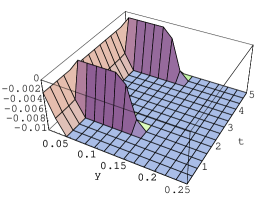
Figure 39: A $=0.01$

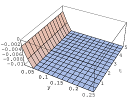
Figure 40: A $=0.001$

On the other hand we wish to consider $\phi$ which has a pole of some order. In particular, the divergent example mention above is dominated by a second order pole near the divergence. One finds in these diverging $\phi$ we get infinite black holes. That is, given some small $\delta$ there is some time before the boundary value diverges at which the sphere of radius $1-\delta$ contains enough energy to form a black hole. In particular, near the divergence $\phi\approx\frac{a}{(\mathrm{t}-\mathrm{t}_{0})^{b}}$. Given $\delta\ll 1,\,\,\delta\ll\frac{(\mathrm{d}-1)(\frac{\mathrm{d}}{2}-1)}{4\pi a^{2}b^{2}(1-2^{1-\frac{\mathrm{d}}{2}})},$ and $\delta\ll\Bigg{(}\frac{4\pi a^{2}b^{2}(1-2^{1-\frac{\mathrm{d}}{2}})}{(\mathrm{d}-1)(\frac{\mathrm{d}}{2}-1)}\Bigg{)}^{\frac{1}{b-1}}$ for $AdS_{\mathrm{d}}(\mathrm{d}\geq 4)$ the expansions in the beginning of the section can be trusted and taking the time $\mathrm{t}=\mathrm{t}_{0}+\Bigg{(}\frac{4\pi a^{2}b^{2}(1-2^{1-\frac{\mathrm{d}}{2}})\delta}{(\mathrm{d}-1)(\frac{\mathrm{d}}{2}-1)}\Bigg{)}^{\frac{1}{2b}}$ upon expanding (5.12) for small $\delta$ one finds there is more than enough energy in a shell from 1 - 2$\delta$ to 1 - $\delta$ to form a black hole of radius 1 - $\delta$. For $AdS_{3}$ taking $\delta\ll 1,\,\,\delta\ll\frac{1}{4\pi a^{2}b^{2}\log{2}},\,\,\delta\log{\delta}\ll\Bigg{(}4\pi a^{2}b^{2}\log{2}\Bigg{)}^{\frac{1}{b-1}}$ and time $\mathrm{t}=\mathrm{t}_{0}+\Bigg{(}4\pi a^{2}b^{2}\log{2}\Bigg{)}^{\frac{1}{2b}}$ leads to the desired conclusion. Then these divergent solutions would seem to produce black holes that swallow up all of space and send the bulk into a big crunch. The gauge theory is apparently well behaved through the transition and so it should be possible to transmit information through at least this kind of collapse. For the cases above after the divergence the dilaton returns to a finite value and at least this author thinks it likely one would have a sensible spacetime on the other side. Definitive statements will require a better understanding of the AdS-FT dictionary.

For small black holes obtaining analytic results seems nontrivial. In particular, the taylor series one would write for small black holes for (5.12) doesn’t converge quickly enough to be useful. However, it is hopefully clear from the form of (5.12) and by the plotted examples that by choosing the parameters in $\phi$ we can determine the size of the black hole we make. The spherically symmetric collapse of matter to form small black holes has been well studied numerically with a line of work started by Matthew Choptuik [6]. These studies start with initial conditions on a spacelike slice but one would expect, especially for boundary conditions which change much faster than the AdS timescale, that one would quickly produce conditions very similiar to that work’s initial conditions and hence reach a similiar conclusion. In particular, the naked singularity found in that work should be resolved by string theory since we have an apparently perfectly well behaved dual quantum field theory.

6 Future Directions

As mentioned before the bulk calculations above are not expected to be qualitatively right because I have not included backreaction. On this point I would like to solicit the attention of numerical relativists. In terms of more basic theoretical issues, one needs a proper definition of asymptotically AdS and energy in the case where one has energy flowing through the boundary. The usual references [7] on this issue assume the energy momentum tensor falls off at infinity faster than one finds in the cases I’ve discussed.

It remains an open question as to how often subtleties such as the ones described above prevent a sensible analytic continuation. Virtually all of the work done on string theory in AdS and AdS/CFT in particular has been done in the Euclidean signature and it would be interesting to know how many more suprises await those examining the Lorentzian case. Regardless, one has from the observations here a whole new AdS-FT dictionary to work out. If this could be done one would almost certainly have many interesting things to say about matter collapsing to form black holes, singularity resolution, and possibly a cosmological bounce. On the other hand, finding even the standard AdS-CFT dictionary has proven to be a nontrivial task. Although not the focus of this paper, using the bulk to study the field theory might also prove interesting; one has a way of at least numerically studying a strongly coupled, non-conformal, non-supersymmetric gauge theory. One might also wonder whether one could find a scattering matrix formalism for the dual field theory in the case where one has a time dependent (although perhaps very slowly varying) gauge coupling. Perturbing boundary conditions provides a rather direct link between the gauge and bulk theories and if we are clever and steadfast enough it may lead to some very interesting physics.

Acknowledgements

I would like to express my appreciation to Gary Horowitz suggesting this project and providing guidance throughout. I’d also like to thank Joe Polchinski for several useful comments.

References

- [1] E. Witten, “Anti De Sitter Space And Holography,” arXiv:hep-th/9802150.
- [2] V. Balasubramanian, P. Kraus, A. Lawrence and S. Trivedi, “Holographic Probes of Anti-de Sitter Spacetimes,” Phys.Rev. D59 (1999) 104021 [arXiv:hep-th/9808017].
- [3] V. Balasubramanian, P. Kraus, and A. Lawrence, “Bulk vs. Boundary Dynamics in Anti-de Sitter Spacetime,” Phys.Rev. D59 (1999) 046003 [arXiv:hep-th/9805171].
- [4] Erdéltyi, A. ed. Higher Transcendental Functions, vol. I McGraw-Hill, 1953.
- [5] D.S. Jones, “Asymptotics of the hypergeometric function,” Mathematical Methods in Applied Science, 2001; 24:369-389
- [6] M. W. Choptuik, “Universality And Scaling In Gravitational Collapse Of A Massless Scalar Field,” Phys. Rev. Lett. 70 (1993) 9. M. W. Choptuik and F. Pretorius, “Gravitational collapse in dimensional AdS spacetime” Phys. Rev. D. 62 (2000) 124012.
- [7] A. Ashtekar and S. Das. “Asymptotically Anti-de Sitter Space-times: Conserved Quantities,” Class.Quant.Grav. 17 (2000) L17-L30 [arXiv:hep-th/9911230]. A. Ashtekar and A. Magnon. “Asymptotically Anti-de Sitter Space-times,” Class.Quant.Grav. 1 (1984) L39