Fatgraph expansion for noncritical superstrings

We study the fatgraph expansion for the Complex Matrix Quantum Mechanics (CMQM) with a Chern-Simons coupling. In the double-scaling limit this model is believed to describe Type 0A superstrings in 1+1 dimensions in a Ramond-Ramond electric field. With Euclidean time compactified, we show that the RR electric field acts as a chemical potential for vortices living on the Feynman diagrams of the CMQM. We interpret it as evidence that the CMQM Feynman diagrams discretize the NSR formulation of the noncritical Type 0A superstring. We also study T-duality for the CMQM diagrams and propose that a certain complex matrix model is dual to the noncritical Type 0B superstring.

CALT-68-2495

1 Introduction

Recently a matrix model description was proposed for Type 0 superstrings in 1+1 dimensions [1, 2]. This proposal realizes an old hope that the double-scaling limit of a matrix model is capable of providing a nonperturbative description of (super)string theory. A particularly intriguing aspect of Refs. [1, 2] is that the matrix models studied there contain only bosonic degrees of freedom, while the dual worldsheet theory contains fermions and is locally supersymmetric (in the NSR formalism). Of course, there is no paradox here, because GSO-projected vertex operators are all bosonic. Nevertheless, it would be much more satisfying if one could give at least a heuristic derivation of the duality on the worldsheet level, similar to that for the 2d bosonic string.

In the case of the bosonic string, the matrix model is a Hermitian Matrix Quantum Mechanics (HMQM) with a potential

$$V(M)=\frac{1}{2}{\rm Tr}M^{2}+\frac{\lambda}{6}\ {\rm Tr}M^{3}$$ (1)

which contains both a quadratic and a cubic piece (see Ref. [3] for a concise review.) If we treat the cubic piece as a perturbation, the free energy of the HMQM can be represented by a sum over trivalent fatgraphs, with Euclidean time variables living on the vertices of the diagrams. Passing to the dual graph, one gets a sum over triangulations of compact 2d surfaces, with the Euclidean time variables living on the faces of the triangulation. In the double-scaling limit, the sum is dominated by triangulations with many faces, and it is plausible that the result is equivalent to 2d gravity coupled to a single scalar field. Thus one concludes that the double-scaled HMQM describes noncritical bosonic string in one dimension. This dimension can be identified with the time of the HMQM. By the usual nonrigorous argument [4], this theory can also be thought of as a critical string theory in 1+1 dimensions.

In this note we discuss fatgraph expansion for the complex Matrix Quantum Mechanics (CMQM). The basic degree of freedom is an $N\times N$ complex matrix, and the action has $U(N)\times U(N)$ invariance. The singlet sector of this model was proposed to be dual to the Type 0A string theory in 1+1 dimensions. The latter theory has only one field-theoretic spacetime degree of freedom, the ”massless tachyon” in the NS-NS sector. It also has a pair of 1-form gauge fields in the RR sector. In 1+1 dimensions 1-forms are not dynamical, but one can contemplate turning on a constant flux (i.e. electric field) for one or both of them. It has been argued in Ref. [2] that in fact only one linear combination of the electric fields can be nonzero, and that turning it on corresponds to working in a sector of the CMQM which is singlet with respect to the $SU(N)\times SU(N)$ subgroup, but has a charge with respect to the $U(1)\times U(1)$ subgroup. More precisely, the ”theta-angle” of the space-time theory was identified with the charge with respect to the difference of the two $U(1)$’s. The theta-angle can be regarded as a chemical potential for the RR electric field. Dually, one can say that the RR electric field is identified with the chemical potential for the aforementioned charge of the CMQM.

An interesting question is how the RR electric field affects the fatgraph expansion of the CMQM free energy. From the worldsheet point of view, RR vertex operators create cuts for worldsheet fermions. If, as in the case of the bosonic string, one can identify fatgraphs with the discretized Type 0A worldsheet in the NSR formalism, then studying the effect of the RR field on the fatgraph expansion could help to “find” fermions in the CMQM.

A convenient way to study the nonsinglet sector of the CMQM is to compactify the Euclidean time and consider twisted boundary conditions in the time direction. The RR electric field then parametrizes the twist matrix. We will show that the Feynman diagrams of the compactified CMQM contain two kinds of vortices, and that the RR electric field is the chemical potential which couples to the difference between the net numbers of vortices of the two kinds. We interpret this as evidence that the CMQM Feynman diagrams provide a discretization of the noncritical Type 0A worldsheet in the NSR formalism. More specifically, we propose that the two kinds of RR vertex operators in Type 0A (usually denoted $(R+,R-)$ and $(R-,R+)$) correspond to two kinds of vortices. We also argue that the scalar field living on the Feynman diagrams of the CMQM is a sum of the worldsheet time and a worldsheet scalar which bosonizes worldsheet fermions.

Another interesting question is the behavior of the fatgraph expansion under T-duality. To discuss T-duality one has to work in Euclidean signature and make the Euclidean time periodic. From the matrix-model point of view, this amounts to studying the canonical partition function of the model. In the bosonic case, one expects that T-duality inverts the periodicity of the Euclidean time, and this can be seen already on the the discretized worldsheet (before taking the double-scaling limit), provided one excludes the contribution of vortices [5, 3]. In the superstring case, we expect T-duality to exchange Type 0A and Type 0B theories. Applying the dualization procedure to the fatgraphs of the CMQM, we will find that the dual Feynman rules can be derived from a certain complex matrix model. We argue that in a suitable scaling limit this model describes Type 0B string theory and explain how this proposal is related with Refs. [1, 2], where the same theory was proposed to be described by an HMQM with an inverted harmonic oscillator potential and symmetric eigenvalue distribution.

2 CMQM and the Type 0A superstring

The CMQM action has the following form:

$$S=\int dt\ {\rm Tr}\left[\frac{dM^{\dagger}}{dt}\frac{dM}{dt}-V(M^{\dagger}M)\right].$$ (2)

Here $M$ is a complex $N\times N$ matrix, and the potential can be taken to be

$$V(x^{2})=m^{2}x^{2}+\frac{\lambda x^{4}}{2}$$ (3)

This theory has $U(N)\times U(N)$ symmetry:

$$M\rightarrow UMV^{-1},\quad U,V\in U(N).$$ (4)

The diagonal $U(1)$ subgroup

$$U(1)_{diag}=\left\{U=V=e^{i\alpha}\cdot{\bf 1}\right\}\subset U(N)\times U(N)$$

acts trivially, so it is more accurate to say that the symmetry group is $G=(U(N)\times U(N))/U(1)_{diag}$. We will denote the anti-diagonal $U(1)$

$$\left\{U=V^{-1}=e^{i\alpha}\cdot{\bf 1}\right\}\subset U(N)\times U(N)$$

by $U(1)_{A}$. The Hilbert space of this theory can be decomposed into irreducible representations of $G$. If one restricts the Hamiltonian to the trivial representation, then the theory becomes equivalent to that of $N$ non-interacting fermions moving on a plane in an external potential $V(|z|^{2})$ and having zero angular momentum [2]. Thus effectively we have non-interacting fermions moving on a half-line. In the double-scaling limit one takes $m^{2}$ to be negative and tunes $m^{2}$ and $\lambda$ so that the Fermi energy is nearly zero, and the number of energy levels below the Fermi level goes to infinity.

The double-scaling limit is believed to describe Type 0A superstring in a simple 1+1-dimensional background; namely, the worldsheet theory is the $N=1$ super-Liouville theory with ${\hat{c}}=9$ plus a free scalar superfield $X$. The lowest component of $X$ is a free scalar $X^{0}$, and translations of this scalar are identified with the time translations in the CMQM. The lowest component of the super-Liouville field $\Phi$ is a scalar $\phi$. The superpartners of $X^{0}$ and $\phi$ will be denoted $\chi,{\bar{\chi}}$ and $\psi,{\bar{\psi}}$, respectively. The worldsheet action on a flat worldsheet is:

$$S=\frac{1}{4\pi}\int d^{2}zd^{2}\theta\left(DX{\bar{D}}X+D\Phi{\bar{D}}\Phi+2i\mu e^{\Phi}\right).$$ (5)

Note that the super-Liouville interaction breaks $(-1)^{F_{L}}$, where $F_{L}$ is the left-moving worldsheet fermion number, but preserves $(-1)^{F}$, where $F=F_{L}+F_{R}$ is the total worldsheet fermion number.

The spectrum of Type 0A superstring consists of a massless tachyon $T$ in the NS-NS sector and a pair of 1-form gauge fields $C,{\tilde{C}}$ in the RR sector. If we denote by $F$ and ${\tilde{F}}$ the corresponding 2-form field-strengths, the RR vertex operators in the $(-1/2,-1/2)$ picture have the following form:

$$V = F(X^{0},\phi)\ c{\bar{c}}\ \exp\left[-\frac{\sigma+{\bar{\sigma}}}{2}+\phi\right]S_{+}{\bar{S}}_{-},$$

$${\bar{V}} = {\tilde{F}}(X^{0},\phi)\ c{\bar{c}}\ \exp\left[-\frac{\sigma+{\bar{\sigma}}}{2}+\phi\right]S_{-}{\bar{S}}_{+}.$$ (6)

Here $\sigma$ and ${\bar{\sigma}}$ are bosonized superconformal ghosts, and $S_{\pm}$ and ${\bar{S}}_{\pm}$ are twist operators for left-moving and right-moving fermions, respectively. In the asymptotic region, where the super-Liouville interaction is negligible, one can bosonize the fermions $\psi,\chi$ and ${\bar{\psi}},{\bar{\chi}}$ into a pair of chiral bosons $H$ and ${\bar{H}}$ and write the twist operators as follows:

$$S_{\pm}=e^{\pm iH/2},\quad{\bar{S}}_{\pm}=e^{\pm i{\bar{H}}/2}.$$ (7)

If we introduce a nonchiral $2\pi$-periodic scalar field $\xi=H+{\bar{H}}$, then RR vertex operators carry unit winding and zero momentum for $\xi$. The 0A GSO projection amounts to keeping only states with zero momentum in the $\xi$ direction. The 0B GSO projection keeps only states with zero winding number in the $\xi$ direction.

Super-Liouville interaction breaks continuous translational invariance for both $\xi$ and its dual. In the language of the original fermions this simply means that rotating $\psi$ into $\chi$ or ${\bar{\psi}}$ into ${\bar{\chi}}$ is not a symmetry. There is still a residual ${\mathbb{Z}}_{2}$ symmetry, generated by $(-1)^{F}$. It flips the sign of all worldsheet fermions.

The super-Virasoro constraints imply that the functions $F$ and ${\tilde{F}}$ are constant. Thus, in the free-field approximation, there are two zero modes corresponding to $F$ and ${\tilde{F}}$. It has been argued in Ref. [2] that the super-Liouville interaction enforces $F_{+}:=F+{\tilde{F}}=0$. Thus there is only one RR zero mode: $F_{-}=F-{\tilde{F}}$. The model admits D0-branes which are charged with respect to $F_{-}$ [6, 7]. These are super-analogues of the so-called ZZ-branes [8]. The D0-brane charge $q$ can be regarded as a theta-angle, or a “chemical potential”, for the RR electric field, in the sense that for fixed $q$ the space-time action contains a term

$$q\int d^{2}x\ F_{-}.$$

However, unlike the theta-angle in ordinary 2d QED, $q$ is integral [2].

On the matrix model side, it was proposed in Ref. [2] that nonzero $q$ corresponds to the sector of the CMQM which is singlet under the $SU(N)\times SU(N)$ subgroup and has $U(1)_{A}$ charge $2qN$. To see that $q$ is integral, recall that both $U(1)_{A}$ and $SU(N)\times SU(N)$ are subgroups of $G=(U(N)\times U(N))/U(1)_{diag}$. This implies a correlation between the $U(1)_{A}$ charge and the transformation properties under the center of $SU(N)\times SU(N)$. In particular, if a representation of $G$ transforms trivially under the $SU(N)\times SU(N)$ subgroup, then its $U(1)_{A}$ charge is divisible by $2N$.

One may enforce the necessary selection rule on the $U(1)_{A}$ charge by gauging the whole $U(N)\times U(N)$ group and adding a Chern-Simons term with a coefficient $q$ to the action:

$$S_{gauged}=\int dt\ {\rm Tr}\left[\frac{DM^{\dagger}}{dt}\frac{DM}{dt}-V(M^{\dagger}M)+iq(A-{\tilde{A}})\right].$$ (8)

Here $A$ and ${\tilde{A}}$ are $U(N)\times U(N)$ gauge fields, and

$$\frac{DM}{dt}=\frac{dM}{dt}+i(AM+M{\tilde{A}}).$$

Then the path integral over $A,{\tilde{A}}$ and $M$ with Euclidean time period $\beta$ computes the following quantity:

$$Z(q)={\rm Tr}\ P_{2qN}\exp(-\beta H_{CMQM}).$$ (9)

Here $P_{qN}$ is the projector onto the subspace which is singlet under $SU(N)\times SU(N)$ and has $U(1)_{A}$ charge equal to $2qN$. If our goal is to understand the effect of the RR electric field on the fatgraphs, it is more useful to work with a “grand canonical ensemble”, whose partition function is given by

$${\hat{Z}}(f)=\sum_{q=-\infty}^{+\infty}Z(q)\exp\left(-iqf\right)$$ (10)

The partition function ${\hat{Z}}(f)$ is computed by a path integral similar to that for $Z_{q}$, except that only the $SU(N)\times SU(N)$ part of the gauge field is integrated over, the $U(1)_{A}$ part of the gauge field is set to zero, and one imposes quasiperiodic boundary conditions on $M$:

$$M(\beta)=e^{2if}M(0).$$ (11)

Following Ref. [9], we may remove the $SU(N)\times SU(N)$ gauge fields from the action by writing

$$A=-i\Omega(t)\frac{d}{dt}\Omega^{-1}(t),\quad{\tilde{A}}=-i{\tilde{\Omega}}(t)\frac{d}{dt}{\tilde{\Omega}}^{-1}(t)$$

for some $SU(N)$-valued functions $\Omega(t),{\tilde{\Omega}}(t)$, satisfying $\Omega(0)={\tilde{\Omega}}(0)=1,$ and performing the corresponding gauge transformation. Then $M(t)$ in the path-integral has the following boundary conditions:

$$M(\beta)=e^{2if}\Omega(\beta)M(0){\tilde{\Omega}}(\beta)^{-1}.$$ (12)

To get ${\hat{Z}}(f)$ one must integrate over the equivalence classes of gauge fields. Since the equivalence class of a gauge field on a circle is completely characterized by the holonomy, we simply have to integrate over $\Omega(\beta)$ and ${\tilde{\Omega}}(\beta)$ using the Haar measure on $SU(N)$. This last description of ${\hat{Z}}(f)$ will be taken as a starting point for developing the fatgraph expansion of the CMQM.

As explained above, $f$ must be identified with $\beta\int dxF_{-}$. The integral in the Liouville direction diverges, and must be regularized by introducing an infrared cut-off. By studying the dependence of the CMQM partition function on the parameter $f$, we will be able to see the effect of the RR electric flux on the discretized worldsheet.

An alternative to the gauged CMQM with a Chern-Simons term is an MQM where the matrix is complex and rectangular (of size $N\times(N+q)$) [2]. The singlet sector of this model is equivalent to the gauged CMQM with a Chern-Simons term. Both are equivalent to the system of planar non-interacting fermions with angular momentum $q$ and subject to an external potential $V(|z|^{2})$. In this paper we do not consider the complex rectangular MQM.

3 Fatgraph expansion for the CMQM

Consider the Euclidean path integral with twisted boundary conditions:

$$Z(\Omega,\tilde{\Omega},f)={\int}_{M(\beta)=e^{2if}\Omega M(0){\tilde{\Omega}}^{\dagger}}\mathcal{D}M(t)\ e^{-Tr\int_{0}^{\beta}dt\left[\partial_{t}M^{\dagger}\partial_{t}M+V(M^{\dagger}M)\right]}$$

where $\Omega$ and $\tilde{\Omega}$ are $SU(N)$ matrices. As explained in the previous section, one can identify $f$ with the RR electric field.

To develop perturbative expansion, we take

$$V(M^{\dagger}M)=M^{\dagger}M+\frac{\lambda}{N}(M^{\dagger}M)^{2}.$$

Expanding the path integral in the parameter $\lambda$, we generate a Feynman diagram expansion.

The propagator for complex $M$ with twisted boundary conditions reads:

$$\langle M_{ik}^{{\dagger}}(t)M_{jl}(0)\rangle_{\beta}=\sum_{m=-\infty}^{\infty}\ e^{-|t+\beta m|}\ e^{2imf}\ (\Omega^{m})_{jk}(\tilde{\Omega}^{-m})_{il},$$

where time ordering is understood on the LHS.

When we expand in the parameter $\lambda$, factors of $Tr(M^{\dagger}M)^{2}$ correspond to vertices, and the propagators are represented by double lines to keep track of the index contractions. Due to the twisting, indices are not conserved along propagator edges, although indices are conserved along an edge at each vertex as shown in Fig. 1. One needs a consistent choice of direction (indicated by small arrows) for each line in the propagator to distinguish lower and upper indices of $M$. Small arrows are “conserved” at the vertices as a consequence of $U(N)\times U(N)$ invariance. One also has to specify an overall direction for each propagator (large arrows) to distinguish the $M$ end from the $M^{\dagger}$ end.

Figure 1: Feynman rule for the propagator.

Since $M^{\dagger}$ has a non-vanishing correlator only with $M$, the large arrows around the boundary of a given face point in the same direction and define an orientation of each face. As always, small arrows determine an orientation for the entire graph which is a Riemann surface. Thus the Feynman diagrams are naturally face-bicolored: a face is colored black or white depending on whether the orientations defined by large and small arrows along its boundary agree or disagree. No two faces sharing an edge can have the same color, since the large arrows will point in opposite directions for them. An example of a Feynman diagram is sketched in Fig. 2. The fact that complex matrix models lead to bicolored graphs is well-known, see Ref. [10] and references therein.

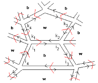
Figure 2: A bicolored Feynman diagram. The relative orientation of large and small arrows determines the color of a face. The matrix indices are shown for some propagators and are not conserved along the propagators due to the twisting.

Rescaling $M\rightarrow\sqrt{N}M$, the propagators acquire an additional factor of $1/N$. Then the weight of a given graph (with a specific coloring of faces) is

$$N^{2-2h}\lambda^{V}\prod_{k}\int_{0}^{\beta}dt_{k}\sum_{m_{ij}}\left(\prod_{white\,faces}\frac{1}{N}{\rm Tr}\ {\tilde{\Omega}}^{w_{f}}\ \prod_{black\,faces}\frac{1}{N}{\rm Tr}\ \Omega^{b_{f}}\ e^{i(w_{f}-b_{f})f}\right)\\ e^{-\sum_{\langle ij\rangle}|t_{i}-t_{j}+\beta m_{ij}|}.$$ (13)

Here $h$ is the genus of the graph, $V$ is the number of vertices, and $w_{f}$ and $b_{f}$ are the “vorticities” of the white ($w$) and black ($b$) faces: $w_{f}=-\sum_{\partial w}m_{ij}$ and $b_{f}=\sum_{\partial b}m_{ij}$.

(Note: it is understood that in the factor $e^{-\sum|t_{i}-t_{j}+\beta m_{ij}|}$ above, the large arrows point from $i$ to $j$ and not vice-versa. This gives precise meaning to the field $m_{ij}$ with respect to which the vorticities are defined. This subtlety appears to have been glossed over in Ref. [9], where this is more pronounced due to the absence of large arrows.)

The link variables $m_{ij}$ can be thought of as an integer-valued gauge field. Gauge transformations are

$$m_{ij}\rightarrow m_{ij}+v_{i}-v_{j},\ t_{i}\rightarrow t_{i}-\beta v_{i}\quad v_{i}\in{\mathbb{Z}}\ \forall i.$$

However, this gauge symmetry is explicitly broken by the finite integration range for $t_{i}$. Therefore, we can extend the integration range for $t_{i}$ to the whole real axis at the expense of gauge-fixing $m_{ij}$. The simplest gauge condition is the “Lorenz gauge”, which requires that at each vertex the sum of all $m_{ij}$ be zero. With this condition imposed, $m_{ij}$ are completely determined by the face vorticities $w_{f}$ and $b_{f}$, and (for $h>0$) vorticities around nontrivial homology cycles of the fatgraph.

In the case of the HMQM, we have a similar expression, except that $\Omega={\tilde{\Omega}}$, and $f=0$. It has been argued [5] that diagrams with nonzero face vorticities are dynamically suppressed in the double-scaling limit, and thus in the singlet sector we might as well set all face vorticities to zero. This is equivalent to saying that in the double-scaling limit it does not matter whether we integrate over the $SU(N)$-valued twist matrices $\Omega={\tilde{\Omega}}$ with the Haar measure, or simply set them to the identity matrix.

In the case of the CMQM, we will assume that sectors which transform nontrivially under $SU(N)\times SU(N)$ are separated from the singlet states by a mass gap, and therefore we can set $\Omega={\tilde{\Omega}}=1$, as in the HMQM. However, Eq. (13) still depends on the face vorticities through the RR electric flux $f$. Thus we cannot ignore vortices even in the double-scaling limit: otherwise the effect of the RR flux would be trivial. We also see that the RR electric field has a simple interpretation in terms of the discretized worldsheet: it is the chemical potential for the difference of black and white vorticities.

In the double-scaling limit the Feynman diagram expansion is dominated by diagrams with a large number of faces. In this limit $t$ can be regarded as a scalar field living on the two-dimensional worldsheet. The discretization of the usual free scalar field action would give

$$\sum_{\langle ij\rangle}(t_{i}-t_{j})^{2}.$$

The action for $t$ that we are getting from the CMQM differs from this in two respects. First, we have to replace $(t_{i}-t_{j})^{2}$ with $|t_{i}-t_{j}|$. It is believed that in the double-scaling limit this does not make any difference [3]. The other difference is that we have to replace $t_{i}-t_{j}$ with

$$t_{i}-t_{j}+\beta m_{ij},$$

which can be thought of as a discretization of

$$\partial_{\mu}t(x)-a_{\mu}(x)$$

where $a_{\mu}$ is a gauge field on the worldsheet. The curvature of the gauge field $a_{\mu}$ is nonzero only at the location of the vortices. Thus we can characterize $a_{\mu}$ by its holonomy around the locations of the vortices (for $h>0$ we also have to specify holonomies around nontrivial homology cycles). A vortex of unit strength is equivalent to

$$\oint a=\beta.$$

We can eliminate $a$ by performing a multi-valued gauge transformation. This has the effect of making the scalar $t(x)$ multivalued: it undergoes a shift by $\beta$ as one goes around any vortex. Summation over $m_{ij}$ is equivalent to summation over all possible vortex insertions. The meaning of this will be discussed in Section 5.

4 T-duality for the discretized superstring worldsheet

In this section we set the RR electric field $f$ to zero, for simplicity. We also set $\Omega={\tilde{\Omega}}=1$, as in the previous section. By performing T-duality on the Feynman diagrams of CMQM, we expect to obtain the Feynman diagrams of a dual matrix model which describes the Type 0B string compactified on the dual circle.

The starting point is the expression for the CMQM partition function ${\hat{Z}}(0)$ derived in the previous section:

$$\log{\hat{Z}}(0)=\sum_{G}N^{2-2h(G)}\lambda^{V}\prod_{k}\int_{0}^{\beta}dt_{k}\prod_{\langle ij\rangle}G(t_{i}-t_{j}).$$ (14)

Here the first sum is over all connected four-valent fatgraphs whose faces are colored black and white, so that as one goes around any vertex, the colors of the adjoining faces alternate. Each vertex is weighed by a factor $\lambda$, and the genus of the fatgraph $G$ is denoted $h(G)$. If we replace the quartic potential in Eq. (3) by a general even polynomial of $M^{\dagger}M$, then the vertices of the fatgraphs will have arbitrary even valence, but the coloring will still alternate.

The last product in Eq. (14) is over all edges of $G$. Each edge contributes the following propagator:

$$G(t_{i}-t_{j})=\sum_{m_{ij}=-\infty}^{+\infty}\exp(-|t_{i}-t_{j}+\beta m_{ij}|).$$

Following Refs. [5, 3], we replace the CMQM propagator with the so-called Villain link factor:

$$G(t_{i}-t_{j})\rightarrow\mathcal{G}(t_{i}-t_{j})=\sum_{m_{ij}=-\infty}^{+\infty}\exp\left(-\frac{1}{2}(t_{i}-t_{j}+\beta m_{ij})^{2}\right).$$

This replacement is believed not to affect the double-scaling limit and allows for a simpler T-duality transformation. The integers $m_{ij}$ live on the edges of the Feynman diagrams and can be regarded as a gauge field. The curl of this gauge fields describes vortices on the worldsheet. Since we set $f=0$, the chemical potential for vortices is zero, and we expect that vortices can be ignored in the continuum [5, 3]. Then $m_{ij}$ is constrained to be curl-free, and on a spherical worldsheet we can write

$$m_{ij}=v_{i}-v_{j},$$

for some integers $v_{i}$. For a worldsheet of genus $g$ one can write:

$$m_{ij}=v_{i}-v_{j}+\epsilon_{ij}^{A}l_{A},\quad v_{i}\in{\mathbb{Z}},\ l_{A}\in{\mathbb{Z}}$$

Here $A$ runs from $1$ to $2h(G)$ and labels arbitrarily chosen 1-cycles of the dual graph representing the basis of the integer homology of the discretized worldsheet. Following Ref. [5], the symbol $\epsilon_{ij}^{A}$ is $\pm 1$ for an edge $\langle ij\rangle$ intersecting the 1-cycle $A$ (the sign depends on their relative orientation), and $0$ otherwise. Summation over $v_{i}$ effectively extends the range of $t_{i}$ to the whole real line. Thus the CMQM free energy becomes:

$$\sum_{G}N^{2-2h(G)}\lambda^{V}\sum_{l_{A}}\prod_{k}\int_{-\infty}^{+\infty}dt_{k}\prod_{\langle ij\rangle}\exp(-\frac{1}{2}(t_{i}-t_{j}+\beta\epsilon_{ij}^{A}l_{A})^{2}).$$

Following Refs. [5, 3], we trade integration over $t_{i}$ for integration over $D_{ij}=t_{i}-t_{j}$. This requires the introduction of a Lagrange multiplier $p_{I}$ for each face of the fatgraph and a Lagrange multiplier $l_{a}$ for each nontrivial homology cycle. Performing the Gaussian integral over $D_{ij}$, we can express the partition function as a sum over dual fatgraphs:

$$\sum_{{\hat{G}}}N^{2-2h(G)}\lambda^{F}\sum_{l_{a}}\prod_{I}\int_{-\infty}^{+\infty}\frac{dp_{I}}{2\pi}\prod_{\langle IJ\rangle}\exp(-\frac{1}{2}(p_{I}-p_{J}+\frac{2\pi}{\beta}\epsilon_{IJ}^{a}l_{a})^{2}).$$

Recall that the fatgraphs of the CMQM have bicolored faces, and as one goes around a vertex, the color of the adjoining faces alternates. In terms of the dual graphs, this means that vertices are colored black and white so that all the nearest neighbors of a black vertex are white, and vice versa (this is known as a bipartite graph). Thus all edges of the dual fatgraph have a natural orientation (from black to white). On each vertex of the dual fatgraph there lives a real-valued scalar $p_{I}$, and the edges are weighed with the Villain factor depending on $p_{I}-p_{J}$. Further, if the original sum runs over four-valent fatgraphs, in the dual fatgraph all faces are quadrangles. If we start with a more general even potential in Eq. (3), then polygons with an arbitrary even number of edges will arise. The valence of the vertices of the dual fatgraph is not constrained.

One can try to reproduce this sum as a Feynman diagram expansion of a matrix model. Since the edges are oriented, it is natural to consider a complex matrix quantum mechanics of a single matrix $P$ with a kinetic term

$$L_{kin}={\rm Tr}\left[\frac{dP^{\dagger}}{dt}\frac{dP}{dt}-P^{\dagger}P\right].$$

For a black vertex, all edges are outgoing, while for a white vertex, they are all incoming. In addition, there is a symmetry which reverses the coloring. To reproduce these Feynman rules, it is natural to try the interaction term

$$L_{int}={\rm Tr}\ W(P)+h.c.,$$

where the function $W$ is a polynomial with real coefficients. The resulting Feynman rules will weigh the vertices, rather than the faces, of the dual fatgraph, but in the continuum limit this should not make much of a difference. (Exactly the same issue arises when studying T-duality for the discretized bosonic string.) The holomorphic potential $W(P)$ is not determined by these considerations. Note that this model has only $U(N)$ gauge-invariance, unlike the CMQM we started from. Unfortunately, it appears impossible to reduce this matrix model to the eigenvalues of $P$. Another problem is that the potential energy is unbounded from below, and it is not clear how to give sense to the path-integral over $P$ beyond perturbation theory. We propose an interpretation in the next section.

5 Discussion

We have seen that the partition function of the CMQM with twisted boundary conditions can be represented as a sum over quadrangulated 2d surfaces, where the vertices are colored black or white, so that every black vertex is surrounded by white ones. On each face of the quadrangulation there lives a real scalar $t$ representing the location of the vertex of the dual graph in Euclidean time. In addition there is a sum over vortices for $t$. These vortices live on the vertices of the quadrangulation and therefore can be labeled as black or white. The total vortex charge must be zero, but the net charge of the black vortices does not have to vanish. The RR electric field is essentially the chemical potential for the charge of the black vortices.

On the other hand, in the NSR formalism the vertex operator for the RR electric field $F_{-}$ is the difference of $V(z,{\bar{z}})$ and ${\bar{V}}(z,{\bar{z}})$ (see Eq. (2)). Thus it is natural to interpret $V$ (resp. ${\bar{V}}$) as corresponding to the insertion of a black (resp. white) vortex on the discretized worldsheet. This identification is supported by the following observation. Consider the worldsheet parity operation $\Omega$. From the worldsheet viewpoint, this operation maps $V$ to $-{\bar{V}}$ and ${\bar{V}}$ to $-V$. From the viewpoint of CMQM, it replaces $M$ with $M^{*}$ [11]. This has the effect of flipping the orientation and reversing the coloring of the quadrangulation (black becomes white and vice versa). In other words, it exchanges black and white vortices and also replaces all vortices by anti-vortices.

From the viewpoint of CMQM, the fact that the vacuum expectation values of $F$ and ${\tilde{F}}$ are always opposite is obvious: this happens because the total vortex charge is always zero.

One interesting aspect of this identification is that the RR vertex operator makes the scalar field $t$, living on the discretized worldsheet, multi-valued. Since the time-like coordinate $X^{0}$ is univalued in the presence of RR vertex operators, this means that the naïve identification of $t$ and $X^{0}$ cannot be correct. Rather, it seems that one has to identify $t$ with the sum $X^{0}+\frac{\beta}{2\pi}\xi$, where the scalar $\xi$ bosonizes the fermions. As one goes around the insertion point of a RR vertex operator, $\xi$ under goes a shift $\xi\rightarrow\xi+2\pi$, and thus $X^{0}+\frac{\beta}{2\pi}\xi$ will shift by $\beta$, as required. Note that $\xi$ does not have a continuous shift symmetry because of the super-Liouville interaction, but $X^{0}$ does. This symmetry corresponds to the time-translation invariance of the CMQM.

As we have mentioned in the introduction, we would like to ”find” the NSR fermions in the matrix model. A weaker form of this problem is to ”find” the sum over spin structures in the fatgraph expansion of the matrix model. The identification of $t$ with $X^{0}+\frac{\beta}{2\pi}\xi$ sheds some light on this issue. In Type 0A theory, summation over spin structures is included in the summation over all possible windings of the periodic scalar $\xi$. In the presence of the Liouville interaction, the winding number symmetry is broken down to ${\mathbb{Z}}_{2}$. Changing the winding of $\xi$ along some 1-cycle on the string worldsheet from even to odd is equivalent to changing the periodicity conditions for worldsheet fermions along this cycle. From the matrix model viewpoint, a winding for $\xi$ translates into a vortex for $t$ as one goes around the corresponding cycle of the discretized worldsheet.

We also discussed T-duality for the discretized Type 0A worldsheet. We found that the dual graphs can be interpreted in terms of a perturbative expansion of a certain complex matrix model with a $U(N)$ invariance. This model does not appear to be soluble for a generic potential.

A different matrix model for the noncritical Type 0B string was proposed in Refs. [1, 2]. In the double-scaling limit, it is an HMQM with a potential of the form

$$V(M)=-M^{2}$$

and eigenvalue density symmetric with respect to zero. This seems to be rather different from what we get by T-dualizing the Type 0A matrix model. Nevertheless, it is possible that the two models describe the same physics in an appropriate continuum limit. Let us sketch a plausible scenario for how this can happen. Recall that in the usual double-scaling limit for the Hermitian matrix model one may replace the potential with an inverted harmonic oscillator potential $V(M)=-M^{2}$. Although this potential is unbounded from below, one can make sense of it by imposing a cut-off on the size of the eigenvalues of $M$. By analogy, let us suppose that the correct scaling limit for our conjectural 0B matrix model is defined by taking $W(P)$ to be quadratic, $W(P)=\alpha P^{2}$. If we write $P=A+iB$, where $A$ and $B$ are Hermitian matrices, then the Lagrangian takes the form

$$L={\rm Tr}\ \left[\left(\frac{dA}{dt}\right)^{2}-(1-2\alpha)A^{2}+\left(\frac{dB}{dt}\right)^{2}-(1+2\alpha)B^{2}\right].$$

The matrices $A$ and $B$ are decoupled. If $\alpha>1/2,$ then $A$ is an inverted harmonic matrix oscillator, while $B$ is an ordinary harmonic matrix oscillator. If $\alpha<-1/2$, then the roles of $A$ and $B$ are reversed. For definiteness, let us choose the first possibility. Then the partition function for $B$ does not have any singularities and can be ignored in the continuum limit. On the other hand, the partition function for $A$, with the cut-off imposed, has a nonanalytic behavior if one tunes $N$ appropriately. In the singlet sector, this nonanalyticity arises when the Fermi-level of the equivalent free-fermion model approaches zero. The continuum limit should correspond to picking the nonanalytic terms in the partition function for $A$. We conclude that in this limit our complex matrix model for $P$ becomes equivalent to the Hermitian matrix model with an inverted harmonic oscillator potential. This agrees with the proposal of Refs. [1, 2].

References

- [1] T. Takayanagi and N. Toumbas, “A matrix model dual of type 0B string theory in two dimensions,” JHEP 0307, 064 (2003) [arXiv:hep-th/0307083].
- [2] M. R. Douglas, I. R. Klebanov, D. Kutasov, J. Maldacena, E. Martinec and N. Seiberg, “A new hat for the c = 1 matrix model,” arXiv:hep-th/0307195.
- [3] I. R. Klebanov, “String theory in two-dimensions,” arXiv:hep-th/9108019.
- [4] A. M. Polyakov, “Quantum Geometry Of Bosonic Strings,” Phys. Lett. B 103, 207 (1981).
- [5] D. J. Gross and I. R. Klebanov, “One-Dimensional String Theory On A Circle,” Nucl. Phys. B 344, 475 (1990).
- [6] T. Fukuda and K. Hosomichi, “Super Liouville theory with boundary,” Nucl. Phys. B 635, 215 (2002) [arXiv:hep-th/0202032].
- [7] C. Ahn, C. Rim and M. Stanishkov, “Exact one-point function of N = 1 super-Liouville theory with boundary,” Nucl. Phys. B 636, 497 (2002) [arXiv:hep-th/0202043].
- [8] A. B. Zamolodchikov and A. B. Zamolodchikov, “Liouville field theory on a pseudosphere,” arXiv:hep-th/0101152.
- [9] V. Kazakov, I. K. Kostov and D. Kutasov, “A matrix model for the two-dimensional black hole,” Nucl. Phys. B 622, 141 (2002) [arXiv:hep-th/0101011].
- [10] P. Di Francesco, “Rectangular Matrix Models and Combinatorics of Colored Graphs,” Nucl. Phys. B 648, 461 (2003) [arXiv:cond-mat/0208037].
- [11] J. Gomis and A. Kapustin, “Two-dimensional unoriented strings and matrix models,” arXiv:hep-th/0310195.