Improved results for ${\cal N}=(2,2)$ super Yang–Mills theory using supersymmetric discrete light-cone quantization

Motomichi Harada^a, John R. Hiller^b, Stephen Pinsky^a, and Nathan Salwen^a

^aDepartment of Physics
Ohio State University
Columbus OH 43210

^bDepartment of Physics
University of Minnesota Duluth
Duluth MN 55812

We consider the (1+1)-dimensional ${\cal N}=(2,2)$ super Yang–Mills theory which is obtained by dimensionally reducing ${\cal N}=1$ super Yang–Mills theory in four dimension to two dimensions. We do our calculations in the large-$N_{c}$ approximation using Supersymmetric Discrete Light Cone Quantization. The objective is to calculate quantities that might be investigated by researchers using other numerical methods. We present a precision study of the low-mass spectrum and the stress-energy correlator $\langle T^{++}(r)T^{++}(0)\rangle$. We find that the mass gap of this theory closes as the numerical resolution goes to infinity and that the correlator in the intermediate $r$ region behaves like $r^{-4.75}$.

1 Introduction

There is a pressing need to solve quantum field theories in the nonperturbative regime. Over the last thirty years a significant amount of progress has been made in this area using lattice gauge theory. Many of the most interesting quantities in QCD and electroweak physics are being calculated to ever increasing accuracy. There remains, however, a number of nonperturbative quantities in supersymmetric quantum field theories that are interesting in a variety of formal physics contexts but have not been calculated. Some of these calculations are now just beginning to be considered. With increased interest in the physics of extra dimensions, it is more important than ever to solve supersymmetric theories in the nonperturbative regime.

The progress in putting supersymmetry on a lattice has been rather slow due to some critical problems: the lack of translational invariance on a lattice, the notorious doubling of fermion states [1], and the breakdown of the Leibniz rule [2]. Recently, however, some interesting new approaches have shed some light on this issue [3, 4, 5, 6]. These approaches make possible the restoration of supersymmetry in a continuum limit without fine-tuning of parameters and even without introducing some “sophisticated” fermions such as domain-wall [7] or overlap fermions [8, 9]. However, these techniques seem to be applicable to only some subset of all supersymmetric theories.

Given this increasing interest and promising new ideas for the realization of supersymmetry on a lattice, it is worthwhile to provide some specific, detailed numerical results using Supersymmetric Discretized Light Cone Quantization (SDLCQ) [10, 11] for the simplest theory for which the new lattice techniques are applicable. SDLCQ is a well established tool for calculations of physical quantities in supersymmetric gauge theory and has been exploited for many supersymmetric Yang–Mills (SYM) theories. The ${\cal N}=(2,2)$ theory in 1+1 dimensions in the large-$N_{c}$ limit is discussed in Ref. [12]; however, the published results are primitive compared to what can be obtained today because of our greatly improved hardware and software. In this paper we are now able to reach a resolution of $K=12$, while in Ref. [12] we could reach only $K=5$. Here we will present new and more detailed results on this theory against which the lattice community can compare the results of their new techniques.

Briefly, the SDLCQ method rests on the ability to produce an exact representation of the superalgebra but is otherwise very similar to Discrete Light Cone Quantization (DLCQ) [13, 14]. In DLCQ we compactify the $x^{-}$ direction by putting the system on a circle with a period of $2L$, which discretizes the longitudinal momentum as $p^{+}=n\pi/L$, where $n$ is an integer. The total longitudinal momentum $P^{+}$ becomes $K\pi/L$, where $K$ is an integer called the harmonic resolution [13]. The positivity of the light-cone longitudinal momenta then limits the number of possible Fock states for a given $K$, and, thus, the dimension of Fock space becomes finite, enabling us to do some numerical computations. It is assumed that as $K$ approaches infinity, the solutions to this large finite problem approach the solutions of the field theory. The difference between DLCQ and SDLCQ lies in the choice of discretizing either $P^{-}$ or $Q^{-}$ to construct the matrix approximation to the eigenvalue problem $M^{2}|\Psi\rangle=2P^{+}P^{-}|\Psi\rangle=2P^{+}(Q^{-})^{2}/\sqrt{2}|\Psi\rangle$, with $P^{+}=K\pi/L$. For more details and additional discussion of SDLCQ, we refer the reader to Ref. [11].

An interesting new result of the calculation we present here is that finite-dimensional representations of the SDLCQ with odd and even values of $K$ result in very distinct solutions of the ${\cal N}=(2,2)$ SYM theory, which only become identical as $K$ approaches infinity. One might initially think that this is a shortcoming of the SDLCQ approach, but it turns out to be an advantage because it provides an internal measure of convergence.

We will give some numerical results of the low-energy spectrum. There we will see that as we go to higher and higher resolutions, we find bound states with lower and lower mass. We have seen this behavior in the ${\cal N}=(1,1)$ theory where the lowest mass state converges linearly to zero as a function of $1/K$. This closing of the mass gap as $K\to\infty$ was predicted by Witten [15] for the ${\cal N}=(1,1)$ and ${\cal N}=(2,2)$ theories. We find that in the latter case the convergence is not linear in $\frac{1}{K}$, and, while our results are consistent with the mass gap going to zero, they are not conclusive.

We have also been able to solve analytically for the wave functions of some of the pure bosonic massless states, and we will present the exact form of the wave function for some cases. We will show that the states must have certain properties to be massless, which then enable us to count the number of the states for a given resolution $K$. In addition, we will present the formulae to count a minimum total number of massless states.

Finally, we will look at the two-point correlation function of the stress-energy tensor $\langle T^{++}(r)T^{++}(0)\rangle$. We see the expected $1/r^{4}$-behavior in the UV and IR regions, and, interestingly, we find that the correlator behaves as $1/r^{4.75}$ in the intermediate region. We know of no predictions for this behavior; however, for ${\cal N}=(8,8)$ SYM theory there is a prediction that this correlator should behave like $1/r^{5}$ in the intermediate region.

The structure of this paper is the following. In Sec. 2 we focus our attention on the low-energy states. After giving a quick review of ${\cal N}=(2,2)$ SYM theory with SDLCQ, we give some numerical results for the low-energy states, discuss analytically some properties of pure bosonic massless states, and present the formulae to count a minimum total number of massless states. We discuss the numerical results for the two-point correlation function of the stress-energy tensor in Sec. 3. A summary and some additional discussion are given in Sec. 4.

2 Review of ${\cal N}$=(2,2) SYM theory

2.1 ${\cal N}$=(2,2) SYM theory and SDLCQ

Before giving the numerical results, let us quickly review some analytical work on ${\cal N}$=(2,2) SYM theory for the sake of completeness. For more details see Ref. [12]. This theory is obtained by dimensionally reducing ${\cal N}$=1 SYM theory from four dimensions to two dimensions. In light cone gauge, where $A_{-}=0$, we find for the action

$$S^{LC}_{1+1} = \int dx^{+}dx^{-}{\rm tr}\Bigg{[}\partial_{+}X_{I}\partial_{-}X_{I}+i\theta^{T}_{R}\partial^{+}\theta_{R}+i\theta^{T}_{L}\partial^{-}\theta_{L}$$

$$\quad+\frac{1}{2}(\partial_{-}A_{+})^{2}+gA_{+}J^{+}+\sqrt{2}g\theta^{T}_{L}\epsilon_{2}\beta_{I}[X_{I},\theta_{R}]+\frac{g^{2}}{4}[X_{I},X_{J}]^{2}\Bigg{]},$$

where $x^{\pm}$ are the light-cone coordinates in two dimensions, the trace is taken over the color indices, $X_{I}$ with $I=1,2$ are the scalar fields and the remnants of the transverse components of the four-dimensional gauge field $A_{\mu}$, two-component spinor fields $\theta_{R}$ and $\theta_{L}$ are remnants of the right-moving and left-moving projections of the four-component spinor in the four-dimensional theory, and $g$ is the coupling constant. We also define the current $J^{+}=i[X_{I},\partial_{-}X_{I}]+2\theta^{T}_{R}\theta_{R}$, and use the Pauli matrices $\beta_{1}\equiv\sigma_{1}$, $\beta_{2}\equiv\sigma_{3}$, and $\epsilon_{2}\equiv-i\sigma_{2}$.

After eliminating all the non-dynamical fields using the equations of motion, we find for $P^{\alpha}=\int dx^{-}T^{+\alpha}$

$$P^{+}=\int dx^{-}{\rm tr}(\partial_{-}X_{I}\partial_{-}X_{I}+i\theta_{R}^{T}\partial_{-}\theta_{R}),$$ (2)

and

$$P^{-}=g^{2}\int dx^{-}{\rm tr}\left(-\frac{1}{2}J^{+}\frac{1}{\partial^{2}_{-}}J^{+}-\frac{1}{4}[X_{I},X_{J}]^{2}+\frac{i}{2}(\epsilon_{2}\beta_{I}[X_{I},\theta_{R}])^{T}\frac{1}{\partial_{-}}\epsilon_{2}\beta_{J}[X_{J},\theta_{R}]\right).$$ (3)

The supercharges are found by dimensionally reducing the supercurrent in the four-dimensional theory. They are

$$Q^{+}_{\alpha}=2^{5/4}\int dx^{-}{\rm tr}(\partial_{-}X_{I}\beta_{I\alpha\eta}u_{\eta}),$$ (4)

$$Q^{-}_{\alpha}=g\int dx^{-}{\rm tr}\left(-2^{3/4}J^{+}\frac{1}{\partial_{-}}\epsilon_{2\alpha\eta}u_{\eta}+2^{-1/4}i[X_{I},X_{J}](\beta_{I}\beta_{J}\epsilon_{2})_{\alpha\eta}u_{\eta}\right),$$ (5)

where $\alpha,\eta=1,2$ and $u_{\alpha}$ are the components of $\theta_{R}$.

We expand the dynamical fields $X_{I}$ and $u_{\alpha}$ in Fourier modes as

$$X_{Ipq}(x^{-})=\frac{1}{\sqrt{2\pi}}\int_{0}^{\infty}\frac{dk^{+}}{\sqrt{2k^{+}}}[A_{Ipq}(k^{+}){\rm e}^{-ik^{+}x^{-}}+A^{{\dagger}}_{Iqp}(k^{+}){\rm e}^{ik^{+}x^{-}}],$$ (6)

$$u_{\alpha pq}(x^{-})=\frac{1}{\sqrt{2\pi}}\int_{0}^{\infty}\frac{dk^{+}}{\sqrt{2}}[B_{\alpha pq}(k^{+}){\rm e}^{-ik^{+}x^{-}}+B^{{\dagger}}_{\alpha qp}(k^{+}){\rm e}^{ik^{+}x^{-}}],$$ (7)

where $p,q=1,2,\ldots,N_{c}$ stand for the color indices, and $A,B$ satisfy the usual commutation relations

$$[A_{Ipq}(k^{+}),A^{{\dagger}}_{Jrs}(k^{{}^{\prime}+})]=\delta_{IJ}\delta_{pr}\delta_{qs}\delta(k^{+}-k^{{}^{\prime}+}),$$ (8)

$$\{B_{\alpha pq}(k^{+}),B^{{\dagger}}_{\beta rs}(k^{{}^{\prime}+})\}=\delta_{\alpha\beta}\delta_{pr}\delta_{qs}\delta(k^{+}-k^{{}^{\prime}+}).$$ (9)

We work in a compactified $x^{-}$ direction of length $2L$ and ignore zero modes. With periodic boundary conditions we restrict to a discrete set of momenta  [10]

$$k^{+}=\frac{\pi}{L}k,\quad k=1,2,3,\ldots,\quad\int dk^{+}\rightarrow\frac{\pi}{L}\sum_{k=1}^{\infty},\quad\delta(k^{+}-k^{\prime+})\rightarrow\frac{L}{\pi}\delta_{k{k^{\prime}}}$$ (10)

Relabeling the operator modes $\sqrt{\frac{L}{\pi}}a(k)=A(k^{+}=\frac{\pi k}{L})$ and $\sqrt{\frac{L}{\pi}}b(k)=B(k^{+}=\frac{\pi k}{L})$, so that

$$[a_{Ipq}(k),a^{{\dagger}}_{Jrs}({k^{\prime}})]=\delta_{IJ}\delta_{pr}\delta_{qs}\delta_{k{k^{\prime}}},\quad\{b_{\alpha pq}(k),b^{{\dagger}}_{\beta rs}({k^{\prime}})\}=\delta_{\alpha\beta}\delta_{pr}\delta_{qs}\delta_{k{k^{\prime}}}.$$ (11)

the expansion is

$$X_{Ipq}(x^{-})=\frac{1}{\sqrt{2\pi}}\sum_{k=1}^{\infty}\frac{1}{\sqrt{2k}}[a_{Ipq}(k){\rm e}^{-i\frac{\pi}{L}kx^{-}}+a^{{\dagger}}_{Iqp}(k^{+}){\rm e}^{i\frac{\pi}{L}kx^{-}}],$$ (12)

$$u_{\alpha pq}(x^{-})=\frac{1}{\sqrt{2L}}\sum_{k=1}^{\infty}\frac{1}{\sqrt{2}}[b_{\alpha pq}(k){\rm e}^{-i\frac{\pi}{L}kx}+b^{{\dagger}}_{\alpha qp}(k){\rm e}^{i\frac{\pi}{L}kx^{-}}].$$ (13)

In terms of $a$ and $b$, the supercharges are given by

$$Q_{\alpha}^{+}=2^{1/4}i\sqrt{\frac{\pi}{L}}\sum_{k=1}^{\infty}\sqrt{k}\beta_{I\alpha\eta}[a^{{\dagger}}_{Iij}(k)b_{\eta ij}(k)-b^{{\dagger}}_{\eta ij}(k)a_{Iij}(k)],$$ (14)

and

$$Q_{\alpha}^{-} = \frac{i2^{-1/4}g}{\pi}\sqrt{\frac{L}{\pi}}\sum^{\infty}_{k_{1},k_{2},k_{3}=1}\delta_{(k_{1}+k_{2}),k_{3}}\Biggl{\{}(\epsilon_{2})_{\alpha\eta}$$

$$\times\Biggl{[}\frac{1}{2\sqrt{k_{1}k_{2}}}\left(\frac{k_{2}-k_{1}}{k_{3}}\right)[b^{{\dagger}}_{\eta ij}(k_{3})a_{Iim}(k_{1})a_{Imj}(k_{2})-a^{{\dagger}}_{Iim}(k_{1})a^{{\dagger}}_{Imj}(k_{2})b_{\eta ij}(k_{3})]$$

$$+\frac{1}{2\sqrt{k_{1}k_{3}}}\left(\frac{k_{1}+k_{3}}{k_{2}}\right)[a^{{\dagger}}_{Iim}(k_{1})b^{{\dagger}}_{\eta mj}(k_{2})a_{Iij}(k_{3})-a^{{\dagger}}_{Iij}(k_{3})a_{Iim}(k_{1})b_{\eta mj}(k_{2})]$$

$$+\frac{1}{2\sqrt{k_{2}k_{3}}}\left(\frac{k_{2}+k_{3}}{k_{1}}\right)[a^{{\dagger}}_{Iij}(k_{3})b_{\eta im}(k_{1})a_{Imj}(k_{2})-b^{{\dagger}}_{\eta im}(k_{1})a^{{\dagger}}_{Imj}(k_{2})a_{Iij}(k_{3})]$$

$$-\frac{1}{k_{1}}[b^{{\dagger}}_{\eta ij}(k_{3})b_{\eta im}(k_{1})b_{\eta mj}(k_{2})+b^{{\dagger}}_{\eta im}(k_{1})b^{{\dagger}}_{\eta mj}(k_{2})b_{\eta ij}(k_{3})]$$

$$-\frac{1}{k_{2}}[b^{{\dagger}}_{\eta ij}(k_{3})b_{\eta im}(k_{1})b_{\eta mj}(k_{2})+b^{{\dagger}}_{\eta im}(k_{1})b^{{\dagger}}_{\eta mj}(k_{2})b_{\eta ij}(k_{3})]$$

$$+\frac{1}{k_{3}}[b^{{\dagger}}_{\eta ij}(k_{3})b_{\eta im}(k_{1})b_{\eta mj}(k_{2})+b^{{\dagger}}_{\eta im}(k_{1})b^{{\dagger}}_{\eta mj}(k_{2})b_{\eta ij}(k_{3})]\Biggr{]}$$

$$+2(\epsilon_{2})_{IJ}\Biggl{(}\frac{1}{4\sqrt{k_{1}k_{2}}}[b^{{\dagger}}_{\alpha ij}(k_{3})a_{Iim}(k_{1})a_{Jmj}(k_{2})+a^{{\dagger}}_{Jim}(k_{1})a^{{\dagger}}_{Imj}(k_{2})b_{\alpha ij}(k_{3})]$$

$$+\frac{1}{4\sqrt{k_{2}k_{3}}}[a^{{\dagger}}_{Jij}(k_{3})b_{\alpha im}(k_{1})a_{Imj}(k_{2})+b^{{\dagger}}_{\alpha im}(k_{1})a^{{\dagger}}_{Jmj}(k_{2})a_{Iij}(k_{3})]$$

$$+\frac{1}{4\sqrt{k_{3}k_{1}}}[a^{{\dagger}}_{Iij}(k_{3})a_{Jim}(k_{1})b_{\alpha mj}(k_{2})+a^{{\dagger}}_{Iim}(k_{1})b^{{\dagger}}_{\alpha mj}(k_{2})a_{Jij}(k_{3})]\Biggr{)}\Biggr{\}}.$$

using the relation $([\beta_{I},\beta_{J}]\epsilon_{2})_{\alpha\eta}=\delta_{\alpha\eta}(\epsilon_{2})_{IJ}$.

They satisfy the superalgebra conditions for anticommutators involving $Q^{+}_{\alpha}$,

$$\{Q^{+}_{\alpha},Q^{+}_{\beta}\}=\delta_{\alpha\beta}2\sqrt{2}P^{+},\quad\{Q^{+}_{\alpha},Q^{-}_{\beta}\}=0.$$ (16)

but do not satisfy the the condition $\{Q^{-}_{\alpha},Q^{-}_{\beta}\}=\delta_{\alpha\beta}2\sqrt{2}P^{-}$. Instead, in SDLCQ we find

$$\{Q^{-}_{\alpha},Q^{-}_{\beta}\}\neq 0\ {\rm if}\ \alpha\neq\beta,\qquad(Q^{-}_{1})^{2}=\sqrt{2}P^{-}_{1}\neq\sqrt{2}P^{-}_{2}=(Q^{-}_{2})^{2}.$$ (17)

Although we have different $P^{-}_{\alpha}$ for different $Q^{-}_{\alpha}$, we can define a unitary, self-adjoint transformation $C$, such that

$$Ca_{1ij}C=a_{2ij},\quad Cb_{1ij}C=-b_{2ij}.$$ (18)

and find that $CP^{-}_{1}C=P^{-}_{2}$. Thus the eigenvalues of $P^{-}_{\alpha}$ are the same. We may choose either one of the two $Q^{-}_{\alpha}$’s, at least for our purposes, and in what follows we will use $Q^{-}_{1}$ and will suppress the subscript unless it is needed for clarity.

The momentum, $P^{+}$, is given by

$$P^{+}=\frac{1}{\sqrt{2}}(Q^{+}_{1})^{2}=\frac{\pi}{L}\sum_{k}k\bigl{(}a_{Iij}^{{\dagger}}a_{Iij}+b_{\nu ij}^{{\dagger}}b_{\nu ij}\bigr{)}$$ (19)

We work with a fixed value of momentum

$$P^{+}=\frac{\pi}{L}K,\quad K=1,2,\ldots$$ (20)

We call $K$ the resolution because larger values of $K$ allow larger values of $L$ while leaving the momentum $P^{+}$ fixed.

The next thing to note is that there are three $Z_{2}$ symmetries of $Q_{1}^{-}$. The first one is $R_{1}$-symmetry, where $R_{\alpha}$ acts as follows

$$a_{1ij}\leftrightarrow a_{2ij},\quad b_{\alpha}\rightarrow-b_{\alpha}$$ (21)

The second is $S$-symmetry

$$a_{Iij}\rightarrow-a_{Iji},\quad b_{\alpha ij}\rightarrow-b_{\alpha ji}.$$ (22)

The third is what we call $T$-symmetry

$$a_{Iij}\rightarrow-a_{Iij},\quad b_{\alpha}\ {\rm unchanged}.$$ (23)

It is easy to see that under these symmetries $Q^{-}_{1}$ is invariant.

Using the relations,

$$R_{1}Q^{+}_{1}R_{1}=-Q_{2}^{+},\quad TQ^{+}_{\alpha}T=-Q^{+}_{\alpha},$$

we find

$$R_{1}(Q^{+}_{1}\pm Q_{2}^{+})R_{1}=\mp(Q^{+}_{1}\pm Q_{2}^{+}),\quad T(Q^{+}_{1}\pm Q_{2}^{+})T=-(Q^{+}_{1}\pm Q_{2}^{+}).$$ (24)

Also note that

$$\{Q^{+}_{1}\pm Q_{2}^{+},Q^{+}_{1}\pm Q_{2}^{+}\}=\{Q^{+}_{1},Q^{+}_{1}\}+\{Q_{2}^{+},Q_{2}^{+}\}+\pm 2\{Q^{+}_{1},Q_{2}^{+}\}=4\sqrt{2}P^{+}.$$ (25)

We work in a subspace of definite momentum so $(Q^{+}_{1}\pm Q_{2}^{+})$ must have non zero eigenvectors. Since $Q^{+}_{\alpha}$ and $Q^{-}_{\alpha}$ are fermionic operators we see that a bosonic energy eigenstate $|\Psi_{B}\rangle_{++}$ which is even under $R$ and $T$-symmetry, can be transformed into

$$|\Psi_{B}\rangle_{\mp-}=Q^{-}_{1}(Q^{+}_{1}\pm Q_{2}^{+})|\Psi_{B}\rangle_{++},\quad|\Psi_{B}\rangle_{-+}=(Q^{+}_{1}+Q^{+}_{2})(Q^{+}_{1}-Q^{+}_{2})|\Psi\rangle_{++}$$ (26)

which are all degenerate with $|\Psi_{B}\rangle_{++}$. One should notice here that we cannot use $Q^{-}_{1}$ and $Q_{2}^{-}$ at the same time since they do not commute with each other. Thus, including the supersymmetry, we have an 8-fold degeneracy. Utilizing the remaining $S$-symmetry, which does not give us a mass degeneracy, we can divide the mass spectrum into 16 independent sectors. This significantly reduces the size of the computational problem. It will be convenient to refer to bound states of this theory as having $S$, $T$, or $R$ even or odd parity and to refer to a state as having even or odd resolutions if $K$ is an even or odd integer.

2.2 Mass gap

Tables 1 and 2 show the first few low-mass states. We find anomalously light states in the sectors with opposite $K$ and $S$ parity for $K$ larger than 4. Furthermore, the number of extremely light states increases by one as we increase $K$ by two. We believe that these anomalously light states should be exactly massless states, but for some reason there is an impediment preventing SDLCQ from achieving this result. Some of the evidence for this comes from a study of the average number of partons $\langle n\rangle$ in the bound states. For example, in the sector with $S$ and $K$ even, for each even integer $r$ less than $K$, there is exactly one bosonic massless state with $\langle n\rangle=r$. For $K$ odd we do not see massless states of this type, but we do find $\langle n\rangle=r$ for the anomalously light bound states in this sector. This is also the first sign of the distinction between representations of the supersymmetry algebra in different symmetry sectors, namely those with anomalously light states (with opposite $S$ and $K$ parity) and those without anomalously light states (with matching $S$ and $K$ parity).

$K$=3	4	5	6	7	8	9	10	11	12
1.308	4.009	0.0067	2.144	0.0040	1.415	0.0026	1.040	0.0018	0.8188
12.62	12.24	0.6304	2.514	0.0060	1.5999	0.0038	1.138	0.0026	0.8790
22.06	15.04	1.0813	2.645	0.4366	1.712	0.0048	1.212	0.0026	0.9312
	15.28	1.1099	2.773	0.6016	1.729	0.3515	1.256	0.0039	0.9397
	22.53	1.5732	2.807	0.6308	1.811	0.4372	1.347	0.3062	1.0072

Table 1: The mass squared $M^{2}$ of the first few lowest massive states in the $S$-even sector in units of $g^{2}N_{c}/\pi$ for a series of resolutions $K$.

$K$=4	5	6	7	8	9	10	11	12
1.2009	3.1876	0.00674	1.8427	0.00440	1.2687	0.00302	0.95786	0.00217
1.2009	3.1887	0.6402	1.9305	0.00538	1.3266	0.00317	0.99795	0.00218
12.296	3.3239	0.6747	2.0413	0.45529	1.4087	0.00431	1.0302	0.00219
12.296	11.489	0.9900	2.1415	0.48010	1.5107	0.36858	1.1036	0.00356
19.502	11.492	1.0313	2.3603	0.55873	1.5219	0.38647	1.1345	0.32053

Table 2: Same as Table 1 but for the $S$-odd sector.

In our discussion of the mass gap we will not include the anomalously light states as part of the massive spectrum for the reason given above. To study the mass gap we will look at the lowest massive state in each sector as a function of $1/K$ as shown in Fig. 1.

(a)	(b)

Figure 1: Plots of the mass squared in units of $g^{2}N_{c}/\pi$ for the lowest massive states, excluding the anomalously light states, with a polynomial fit constrained to go through the origin. The plot in (a) corresponds to the sector where $S$ and $K$ have the same parity, and the plot in (b) to the sector where $S$ and $K$ have opposite parity.

There we also show polynomial fits in all four sectors separately. The fits are constrained to go through the origin. The quadratic fits look very good in Fig. 1(a). but Fig. 1(b) required a cubic. The two fits with opposite $S$ and $K$ parity look very similar as do the two fits with same $S$ and $K$ parity. In each case we could have fit all the points with one curve if we were to include a small oscillatory function in the fit. We should note here that oscillatory behavior has been observed before in different theories [16, 17]. The explanation given there is that those states which show the oscillatory behavior comprise non-interacting two-body states. This, however, does not seem applicable in our case since the states in Fig. 1 are the lowest energy states; thus there are no lower energy states available to form two-body states.

The distinct character of the mass gap serves as another piece of evidence that we have two different classes of representations. The data is consistent with the mass gap closing to $0$ as $K\to\infty$, especially for the case where $S$ and $K$ have the same parity. The odd and even representations approach each other as $K$ increases and we hypothesize that they become identical in the continuum limit of $K\to\infty$. When we present the correlation function in Sec. 3, we will see further evidence for this claim.

2.3 Massless states

2.3.1 Pure bosonic massless states

Let us investigate the properties of pure bosonic massless states in full detail in the $N_{c}\to\infty$ limit. This is done by generalizing the discussion of the bound states in SDLCQ for ${\cal N}$=(1,1) SYM theory, as given in Refs. [11, 18], to ${\cal N}$=(2,2) SYM theory.

For simplicity, let us consider the states consisting of a fixed $n$ number of partons only. A pure bosonic massless state is given by

$$|\Psi,0\rangle=N\sum_{q_{1},\ldots,q_{n}}\sum_{A}\delta_{(q_{1}+\ldots+q_{n}),K}\bar{f}^{(0)}_{[A_{1}\ldots A_{n}]}(q_{1}\ldots q_{n}){\rm tr}[a_{A_{1}}^{{\dagger}}(q_{1})\ldots a_{A_{n}}^{{\dagger}}(q_{n})]|0\rangle,$$

where $N$ is the normalization factor, $q_{i}=1,2,\ldots$ is the unit of the light-cone momentum $p_{i}=q_{i}\pi/L$ carried by the $i$-th parton, $A_{i}=1,2$ indicates the flavor index for each parton, the sum $\sum_{A}$ is the summation over all possible permutations of the flavor indices $A_{i}$’s, $\bar{f}$ is the wave function, and the trace is taken over the color indices. Note that we don’t have the symmetry factor coming from the cyclic property of the trace in the above notation; one has to put in the symmetry factor by hand if one would like it to be in there as we will do so for an example given later in this subsection. In other words, Fock states with non-zero symmetry factor are not normalized.

Due to the cyclic property of the trace, we have

$$\bar{f}_{[A_{1}\ldots A_{n}]}(q_{1},\ldots,q_{n})=\bar{f}_{[A_{2}\ldots A_{n}A_{1}]}(q_{2},\ldots,q_{n},q_{1})=\ldots=\bar{f}_{[A_{n}A_{1}\ldots A_{n-1}]}(q_{n},\ldots,q_{n-1}).$$

Since $P^{-}=(Q^{-})^{2}/\sqrt{2}$, all the massless states should vanish upon the action of $Q^{-}$. Thus, we must have $Q^{-}|\Psi,0\rangle=0$. This identity, however, can be simplified somewhat for pure bosonic massless states. That is, the terms to consider in $Q^{-}$ are those which annihilate one boson and create one boson and one fermion, and those which annihilate two bosons and create one fermion. Both the former and latter class of terms in $Q^{-}$ separately annihilates $|\Psi,0\rangle$. In the large-$N_{c}$ limit the former class gives, writing $f(q_{1},\ldots,q_{n})\equiv\sqrt{q_{1}\ldots q_{n}}\bar{f}(q_{1},\ldots,q_{n})$,

$$0 =(\epsilon_{2})_{\alpha\beta}\Bigl{\{}\frac{2q_{n-1}+t}{(q_{n-1}+t)t}f^{(0)}_{[A_{1}\ldots A_{n}]}(q_{1},\ldots,q_{n-1}+t,q_{n})$$ (27)

$$\quad-\frac{2q_{n}+t}{(q_{n}+t)t}f^{(0)}_{[A_{1}\ldots A_{n}]}(q_{1},\ldots,q_{n-1},q_{n}+t)\Bigl{\}}$$

$$\quad+\frac{M_{IA_{n}}^{\alpha\beta}}{2(q_{n}+t)}f^{(0)}_{[A_{1}\ldots A_{n-1},I]}(q_{1},\ldots,,q_{n-1},q_{n}+t)$$

$$\quad-\frac{M_{IA_{n-1}}^{\alpha\beta}}{2(q_{n-1}+t)}f^{(0)}_{[A_{1}\ldots A_{n-2},I,A_{n}]}(q_{1},\ldots,,q_{n-1}+t,q_{n}),$$

and the latter yields

$$0=\sum_{A_{n-1},A_{n}}\sum_{k}\left((\epsilon_{2})_{\alpha\beta}\frac{t-2k}{tk(t-k)}\delta_{A_{n-1},A_{n}}+\frac{M_{A_{n-1}A_{n}}^{\alpha\beta}}{k(t-k)}\right)f^{(0)}_{[A_{1}\ldots A_{n}]}(q_{1},\ldots,q_{n-2},k,t-k),$$ (28)

where $M_{IJ}^{\alpha\beta}\equiv[(\beta_{I}\beta_{J}-\beta_{J}\beta_{I})\epsilon_{2}]_{\alpha\beta}$, $t$ is the momentum of the created fermion, and the momentum conserving Kronecker’s delta $\delta_{(q_{1}+\ldots+q_{n}),K}$ is understood implicitly. These are the necessary and sufficient conditions for a pure bosonic state to be massless. One should notice that the above equations reduce to the corresponding equations found in Ref. [11, 18] with $(\epsilon_{2})_{\alpha\beta}=1$, $A_{i}=1$ for all $i$’s, and $M_{IJ}^{\alpha\beta}=0$, as expected.

In principle, we could find the properties of all kinds of pure bosonic massless states using Eqs. (27) and (28). However, we limit ourselves here to the investigation of only two special types. To simplify the notation, we omit the superscript $(0)$ from the wave function $f$ hereafter.

The simplest case is where $n=K$, that is to say, all the partons have one unit of momentum $\pi/L$ and, thus, $f=\bar{f}$. In this case Eq. (27) is trivially satisfied since we cannot have states with $(K+1)$ partons. From Eq. (28) we get

$$0=f_{[A_{1}\ldots A_{n-2},1,2]}-f_{[A_{1}\ldots A_{n-2},2,1]},$$ (29)

where we have omitted $(q_{1},\ldots,q_{n})=(1,\ldots,1)$. Eq. (29) means, with the help of the cyclic property of $f$, that the wave function is unchanged after moving any flavor index to any location in the list of indices. For instance, we find, writing $f_{[A_{1}\ldots A_{n}]}\equiv[A_{1}\ldots A_{n}]$,

$$[1212]=[1221]=[2121]=[2211]=[2112]=[1122].$$

It is clear that the state with the above six wave functions being the same and all others zero satisfies (29), or equivalently Eqs. (27) and (28), the necessary and sufficient conditions to be massless. Therefore, writing ${\rm tr}[a^{{\dagger}}_{A_{1}}(1)\ldots a^{{\dagger}}_{A_{n}}(1)]|0\rangle\equiv A_{1}\ldots A_{n}$, we find the state

$$N[1212](1212+1221+2121+2211+2112+1122)=N[1212](2(1212)+4(1122))$$

is massless, where we used the cyclic property of $f$. In terms of the normalized Fock states ${\rm tr}[a^{{\dagger}}_{A_{1}}(1)\ldots a^{{\dagger}}_{A_{n}}(1)]|0\rangle/(\sqrt{s}N_{c}^{n/2})\equiv\underline{A_{1}\ldots A_{n}}=A_{1}\ldots A_{n}/(\sqrt{s}N_{c}^{n/2})$, where $s$ is the symmetry factor, we find, after normalizing properly, that

$$\frac{1}{\sqrt{3}}(\underline{1212})+\sqrt{\frac{2}{3}}(\underline{1122})$$

is massless since $s$ for 1212 and 1122 equals two and one, respectively. Indeed we have found the very same massless state in our numerical results.

As we have seen above, there is a one-to-one correspondence between a massless state and a given set of flavor indices, which has a fixed number of 1’s and 2’s. This means that every time we change the number of 1’s (or 2’s) in the flavor indices, we find a new massless state. Since we can have $K+1$ such different sets of flavor indices, we have $K+1$ massless states of this kind. As verification of our argument, we enumerated all the massless states for $K$ up to six and found all of them with the correct coefficients in our numerical results.

The next case to consider is where $n=K-1$. In this case only one of the partons has two units of momentum, so that $f=\sqrt{2}\bar{f}$. However, since all the $f$’s have the same factor of $\sqrt{2}$, we can absorb $\sqrt{2}$ into the normalization factor $N$ and practically can set $f\equiv\bar{f}$. We have $t=1$ and $q_{i}=1$ with $i=1,\ldots,n$ in Eq. (27) and find, writing $(q_{1},\ldots,q_{n})=(1,\ldots,1,1,2)\equiv(1,2)$ and so on,

$$0=[A_{1}\ldots A_{n}](2,1)-[A_{1}\ldots A_{n}](1,2),$$ (30)

$$0=[A_{1}\ldots A_{n-2},A_{n-1},A_{n}](1,2)-[A_{1}\ldots A_{n-2},A_{n},A_{n-1}](2,1),$$ (31)

$$0=[A_{1}\ldots A_{n-2},A_{n-1},A_{n-1}](1,2)+[A_{1}\ldots A_{n-2},A_{n},A_{n}](2,1),$$ (32)

where $A_{n-1}\neq A_{n}$ in Eqs. (31) and (32). For Eq. (28) we have $t=2$, $k=1,2$ and $q_{i}=1$ with $i=1,\ldots,n-2$, and we get

$$0=[A_{1}\ldots A_{n-2},A,A](1,2)-[A_{1}\ldots A_{n-2},A,A](2,1),$$ (33)

$$0 = [A_{1}\ldots A_{n-2},1,2](1,2)+[A_{1}\ldots A_{n-2},1,2](2,1)$$ (34)

$$\quad-[A_{1}\ldots A_{n-2},2,1](1,2)-[A_{1}\ldots A_{n-2},2,1](2,1).$$

Apparently, we have five equations for the massless states to satisfy, but it is easy to see that Eq. (33) is incorporated into Eq. (30) and that if Eqs. (30) and (31) are true, so is Eq. (34) automatically. Hence, the three equations Eqs. (30), (31), and (32) are in fact the equations for massless states to satisfy for $n=K-1$.

In order to see what the three equations allow us to do, let us first write

$$[A_{1},\ldots,A_{n}](1,2)\equiv[A_{1},\ldots,A_{n}^{\prime}].$$

That is, let us put a prime on top of an index whose corresponding parton has two units of momentum. Then, Eq. (30) allows us to move the “prime” to any index. Eq. (31), along with this fact, then also allows us to move the index with a prime to any location in the index list. For example, we have

$$[112^{\prime}]=[11^{\prime}2]=[1^{\prime}12]=[12^{\prime}1]=[1^{\prime}21]=[121^{\prime}]=[2^{\prime}11]=[21^{\prime}1]=[211^{\prime}].$$

Furthermore, Eq. (32) allows us to replace $11^{\prime}$ by $2^{\prime}2$ (or $22^{\prime}$ using Eq. (30)) as long as a minus sign is inserted. Thus, for the above example we get

$$[112^{\prime}]=[11^{\prime}2]=[1^{\prime}12]=-[22^{\prime}2],$$

where we have omitted the wave functions related by cyclic permutations. This means that the state

$$(112^{\prime}+11^{\prime}2+1^{\prime}12-22^{\prime}2)/2$$

is massless. Note that the symmetry factor in this case is equal to one for all the Fock states above.

Since Eqs. (30), (31), and (32) relate all the sets of flavor indices with an even/odd number of 1’s to one another, we have only two independent sets of flavor indices: the one with even numbers of 1’s and the other with an odd number. This means that there are two massless states of this type. Again we have confirmed this statement numerically for $K$ up to six.

To summarize, we have found in the large-$N_{c}$ limit the necessary and sufficient conditions, Eqs. (27) and (28), that pure bosonic massless states are to satisfy. As an application we considered two special cases and found that there are $K+1$ massless states of the type ${\rm tr}[a^{{\dagger}}_{A_{1}}(1)\ldots a^{{\dagger}}_{A_{K}}(1)]$ and two of the type ${\rm tr}[a^{{\dagger}}_{A_{1}}(1)\ldots a^{{\dagger}}_{A_{K-2}}(1)a^{{\dagger}}_{A_{K-1}}(2)]$. Also, we gave a way to enumerate all such massless states for a given $K$.

2.3.2 Count of massless states

It is possible to predict a minimum number of massless states by comparing the number of states in the different symmetry sectors. Since $(Q^{-})^{2}$ takes a state from one symmetry sector to another and then back it must have $0$ eigenvalues if the dimensionality of the intermediate sector is less than that of the original sector. It is possible to create a simple recursive formula for the number of states in each sector[19]. For the case when $K$ is prime and odd, the formula is particularly simple. We present the results here but refer to the other publication for justification. We define $A_{bes^{+}}(K,n)$ as the number of states in the bosonic sector with an even number of partons and even $S$ symmetry, where $n$ indicates how many types of particles we have in a SYM theory, i.e. $n=4$ for ${\cal N}=(2,2)$ SYM. Then

$$A_{bes^{+}}(K,n)=A_{fes^{+}}(K,n)=\frac{A_{f}(K,n)+A_{f}(K,-n)+W}{2}$$ (35)

$$A_{bes^{-}}(K,n)=A_{fes^{-}}(K,n)=\frac{A_{f}(K,n)+A_{f}(K,-n)-W}{2}$$

$$A_{bos^{+}}(K,n)=A_{fos^{+}}(K,n)=A_{bos^{-}}(K,n)=A_{fos^{-}}(K,n)=\frac{A_{f}(K,n)-A_{f}(K,-n)}{2}$$

where

$$A_{f}(K,n)_{\hbox{prime}}=\frac{1}{2K}((1+n)^{K}-(1+n))$$ (36)

$$W=(\frac{n}{2})^{2}(K-1)$$ (37)

$Q^{-}$ goes from bosonic to fermionic and from even to odd.

$$A_{fos^{+}}(K,n)-A_{bes^{+}}(K,n)=A_{bos^{+}}(K,n)-A_{fes^{+}}(K,n)=-A_{f}(K,-n)-\frac{W}{2}$$ (38)

$$A_{fos^{-}}(K,n)-A_{bes^{-}}(K,n)=A_{bos^{-}}(K,n)-A_{fes^{-}}(K,n)=-A_{f}(K,-n)+\frac{W}{2}$$ (39)

The minimum total number of massless states must therefore be

$$-4A_{f}(K,-n)=-\frac{2}{K}((1-n)^{K}-(1-n))=\frac{2}{K}(3^{K}-3)$$ (40)

For $K=5$, this comes to $96$ states which is way more than the $8$ purely bosonic states with $4$ or $5$ partons that we have found in this section.

3 Correlation functions

One of the physical quantities we can calculate nonperturbatively is the two-point function of the stress-energy tensor. Previous calculations of this correlator in this and other theories can be found in [20, 21, 22]. Ref. [20] gives results for the theory considered here but only for resolutions $K$ up to 6. We can now reach $K=12$.

We will show that there is a distinct behavior for even and odd $K$ in the correlation function, just as in the energy spectrum. Then we will argue, by taking a closer look at the data, that we have two different classes of representations at finite $K$, which become identical as $K\to\infty$.

3.1 Correlation functions in supergravity

Let us first recall that there is a duality that relates the results for the two-point function in ${\cal N}$=(8,8) SYM theory to the results in string theory [21]. The correlation function on the string-theory side, which can be calculated with use of the supergravity approximation, was presented in [20], and we will only quote the result here. The computation is essentially a generalization of that given in [23, 24]. The main conclusion on the supergravity side was reported in [25]. Up to a numerical coefficient of order one, which we have suppressed, it was found that

$$\langle{\cal O}(x){\cal O}(0)\rangle=\frac{N_{c}^{\frac{3}{2}}}{g_{YM}x^{5}}.$$ (41)

This result passes the following important consistency test. The SYM theory in two dimensions with 16 supercharges has conformal fixed points in both the UV and the IR regions, with central charges of order $N_{c}^{2}$ and $N_{c}$, respectively. Therefore, we expect the two-point function of the stress-energy tensor to scale like $N_{c}^{2}/x^{4}$ and $N_{c}/x^{4}$ in the deep UV and IR regions, respectively. According to the analysis of [26], we expect to deviate from these conformal behaviors and cross over to a regime where the supergravity calculation can be trusted. The crossover occurs at $x=1/g_{YM}\sqrt{N_{c}}$ and $x=\sqrt{N_{c}}/g_{YM}$. At these points, the $N_{c}$ scaling of (41) and the conformal result match in the sense of the correspondence principle [27].

We should note here that this property for the correlation functions is expected only for ${\cal N}$=(8,8) SYM theory, not for the theory in consideration in this paper. However, it would be natural to expect some similarity between ${\cal N}$=(8,8) and ${\cal N}$=(2,2) theories. Indeed, we will find numerically that (41) is almost true in ${\cal N}$=(2,2) SYM theory.

3.2 Correlation functions in SUSY with 4 supercharges

We wish to compute a general expression of the form $F(x^{-},x^{+})=\langle{\cal O}(x^{-},x^{+}){\cal O}(0,0)\rangle$ where ${\cal O}$ is $T^{++}$. In DLCQ, where we fix the total momentum in the $x^{-}$ direction, it is more natural to compute the Fourier transform and express the transform in a spectral decomposed form [20, 21]

$$\tilde{F}(P_{-},x^{+})=\frac{1}{2L}\langle{T^{++}}(P_{-},x^{+}){T^{++}}(-P_{-},0)\rangle$$

$$=\sum_{i}\frac{1}{2L}\langle 0|{T^{++}}(P_{-},0)|i\rangle{\rm e}^{-iP^{i}_{+}x^{+}}\langle i|{T^{++}}(-P_{-},0)|0\rangle.$$ (42)

The position-space form of the correlation function is recovered by Fourier transforming with respect to $P_{-}=P^{+}=K\pi/L$. We can continue to Euclidean space by taking $r=\sqrt{2x^{+}x^{-}}$ to be real. The result for the correlator of the stress-energy tensor was presented in [20], and we only quote the result here:

$$F(x^{-},x^{+})\equiv\langle T^{++}({\bf x})T^{++}(0)\rangle=\sum_{i}\Big{|}\frac{L}{\pi}\langle 0|T^{++}(K)|i\rangle\Big{|}^{2}\left(\frac{x^{+}}{x^{-}}\right)^{2}\frac{M_{i}^{4}}{8\pi^{2}K^{3}}K_{4}(M_{i}\sqrt{2x^{+}x^{-}}),$$ (43)

where ${\bf x}$ has light cone coordinates $x^{-},x^{+}$, $M_{i}$ is a mass eigenvalue and $K_{4}(x)$ is the modified Bessel function of order 4. In [12] we found that the momentum operator $T^{++}({\bf x})$ is given by

$$T^{++}({\bf x})={\rm tr}\left[(\partial_{-}X^{I})^{2}+\frac{1}{2}(iu^{\alpha}\partial_{-}u^{\alpha}-i(\partial_{-}u^{\alpha})u^{\alpha})\right],\quad I,\alpha=1,2,$$ (44)

where $X$ and $u$ are the physical adjoint scalars and fermions, respectively, following the notation of [12]. When written in terms of the discretized operators, $a$ and $b$, (Eqs. (12,13)), we find

$$T^{++}(K)|0\rangle=\frac{\pi}{2L}\sum_{k=1}^{K-1}$$

$$\quad\left[-\sqrt{k(K-k)}a^{{\dagger}}_{Iij}(K-k)a^{{\dagger}}_{Iji}(k)+\left(\frac{K}{2}-k\right)b^{{\dagger}}_{\alpha ij}(K-k)b^{{\dagger}}_{\alpha ji}(k)\right]|0\rangle.$$ (45)

The matrix element $(L/\pi)\langle 0|T^{++}(K)|i\rangle$ is independent of $L$ and can be substituted directly to give an explicit expression for the two-point function. We see immediately that the correlator behaves like $1/r^{4}$ at small $r$, for in that limit, it asymptotes to

$$\left(\frac{x^{-}}{x^{+}}\right)^{2}F(x^{-},x^{+})=\frac{N_{c}^{2}(2n_{b}+n_{f})}{4\pi^{2}r^{4}}\left(1-\frac{1}{K}\right).$$ (46)

On the other hand, the contribution to the correlator from strictly massless states is given by

$$\left(\frac{x^{-}}{x^{+}}\right)^{2}F(x^{-},x^{+})=\sum_{i}\Big{|}\frac{L}{\pi}\langle 0|T^{++}(K)|i\rangle\Big{|}^{2}_{M_{i}=0}\frac{6}{K^{3}\pi^{2}r^{4}}.$$ (47)

That is to say, we would expect the correlator to behave like $1/r^{4}$ at both small and large $r$, assuming massless states have non-zero matrix elements.

3.3 Numerical results

To compute the correlator using Eq. (43), we approximate the sum over eigenstates by a Lanczos [28] iteration technique, as described in [21, 22]. Only states with positive $R_{\alpha}$, $T$ and $S$ parity contribute to the correlator. The results are shown in Fig. 2, which includes a log-log plot of the scaled correlation function

$$f\equiv\langle T^{++}({\bf x})T^{++}(0)\rangle\left(\frac{x^{-}}{x^{+}}\right)^{2}\frac{4\pi^{2}r^{4}}{N_{c}^{2}(2n_{b}+n_{f})}$$ (48)

and a plot of $d\log_{10}(f)/d\log_{10}(r)$ versus $\log_{10}(r)$, with $r$ measured in units of $\sqrt{\pi/g^{2}N_{c}}$. Let us discuss the behavior of the correlator at small, large, and intermediate $r$, separately in the following.

First, at small $r$, the graphs of $f$ for different $K$ approach 0 as $K$ increases. This follows Eq. (46) which gives the form $f=\log(1-\frac{1}{K})$. Second, at large $r$, obviously, the behavior is different for odd $K$, in Fig. 2(c) and (d), and even $K$, in (e) and (f). However, the difference gets smaller as $K$ gets bigger, as seen in Fig. 2(a). The reason for this is as follows. Looking at the detailed information of the computation of the correlator, we found that for even $K$ there is exactly one massless state that contributes to the correlator, while there is no massless state nor even an anomalously light state that makes any contribution for odd $K$. Instead, it is the lowest massive state that contributes the most for odd $K$. This observation serves as another piece of evidence for the claim that we have two distinct classes of representations for odd and even $K$.

In the intermediate-$r$ region, for the ${\cal N}$=(8,8) theory we expected from Eq. (41) that the behavior is $1/r^{5}$, and in [21] we found that the correlator may be approaching this behavior. We indicated in [21] that conclusive evidence would be a flat region in the derivative of the scaled correlator at a value of $-1$. Our resolution was not high enough to see this in the ${\cal N}$=(8,8) case. Here we find such a flat region, indicating that the correlator in fact behaves like $1/r^{-4.75}$ for ${\cal N}$=(2,2) SYM theory. Also, note that the region of flattening around $-0.75$ extends farther out as $K$ gets bigger, for both odd and even $K$, implying again that the representations appear to agree as $K$ goes to infinity. For any fixed value of $r$ the correlators for odd and even $K$ approach each other as $K$ increases and the flat region extends further. This indicates that it is only in the region of $r$ where the correlators for even and odd $K$ agree that we have sufficient convergence for the results to be meaningful.

(a)	(b)
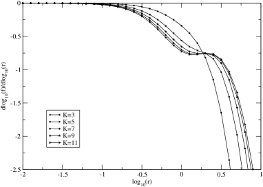
(c)	(d)
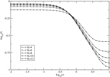
(e)	(f)

Figure 2: Plots of log of the scaled correlation function $f$ as a function of $\log_{10}(r)$ for (a) $K=3,4,\ldots 12$, (c) $K$ odd, and (e) $K$ even, and plots of $d\log_{10}(f)/d\log_{10}(r)$ as a function of $\log_{10}(r)$ for (b) $K=3,4,\ldots 12$, (d) $K$ odd, and (f) $K$ even.

4 Discussion

To respond to the increasing interest in calculating supersymmetric theories on a lattice [3, 4, 5, 6], we have presented detailed numerical results for the low-energy spectrum and the two-point correlation function of the stress-energy tensor, using SDLCQ for ${\cal N}$=(2,2) SYM theory in $1+1$ dimensions in the large-$N_{c}$ approximation. Our hope is that these results will serve as benchmarks for others to compare and check their results.

In addition, we found an important new aspect of the SDLCQ approximation in this calculation. There seem to be two distinct classes of representations for ${\cal N}$=(2,2) SYM theory, one where $S$ and $K$ have the same parity and one where $S$ and $K$ have opposite parity; these representations become identical as $K\to\infty$. We found evidence for this feature of ${\cal N}$=(2,2) SYM theory in both the mass spectrum and the correlator. We also found that there are some anomalously light states that appear only in the sectors where $S$ and $K$ have opposite parity. We argued that the anomalously light states should be exactly massless, but have acquired a tiny mass because of some impediment to having them exactly massless in the SDLCQ approximation. In the calculation of the correlator where only positive S parity contribute we found that there is exactly one massless state that contributes to the correlator when $K$ has positive parity and that no massless state or anomalously light state contributes when $K$ has negative parity. The lightest massive state in the sector where $K$ has negative parity does contribute to the correlator, but because the mass gap appears to close at infinite resolution this state appears to become massless, as expected [15].

The two-point correlator of the stress-energy tensor was found to show $1/r^{4}$-behavior in the UV (small $r$) and IR (large $r$, $K$ even) regions as expected. The large $r$ behavior for $K$ odd, on the other hand, has an exponential decay. Surprisingly, the correlator behaves like $1/r^{4.75}$ at intermediate values of $r$. In ${\cal N}$=(8,8) SYM theory in $1+1$ dimensions, the correlator is expected to behave like $1/r^{5}$ in the intermediate region, and it is interesting that ${\cal N}$=(2,2) behaves similarly but with a different exponent. We were able to confirm this power law behavior with a flat region in the derivative of the scaled correlator. Previously, in our calculation of the ${\cal N}$=(8,8) correlator at lower resolutions, we were not able to find this flat region. We are hopeful that in the near future we may be able to conclusively confirm the $1/r^{5}$ behavior in the ${\cal N}$=(8,8) theory. Interestingly, we also note that earlier results seem to indicate the same type of odd/even behavior for the ${\cal N}$=(8,8) theory.

Analytically, we investigated the properties of pure bosonic massless states and found the necessary and sufficient conditions to determine their wave function. Then we explored some special cases to find that there are $K+1$ massless states of type

$${\rm tr}[a_{A_{1}}^{{\dagger}}(1)a_{A_{2}}^{{\dagger}}(1)\ldots a_{A_{K}}^{{\dagger}}(1)]|0\rangle,$$

where $A_{i}$ is a flavor index and the number in the parentheses tells how many units of momentum each parton carries, and that there are two massless states of the type

$${\rm tr}[a_{A_{1}}^{{\dagger}}(1)a_{A_{2}}^{{\dagger}}(1)\ldots a_{A_{K-1}}^{{\dagger}}(2)]|0\rangle.$$

We also gave the formulae to count a minimum total number of massless states for a SYM theory which is demensionally reduced to one spatial and one time dimensions.

What prevents us from reaching even higher $K$ is obviously the fact that, as one can show [19], the total number of basis states grows like $\sim(1+n)^{K}$, where $n$ is the total number of particle types and $n=4$ for ${\cal N}$=(2,2) SYM theory. Our numerical results were obtained using one single PC with memory of 4 GB. The problem that we now face is that we do not have enough memory to store all the states in one PC. However, as we make use of a cluster of PCs and find ways to split and share the information among them, we are able to reach even higher $K$. This is the direction of our future work, with the ultimate goal being to achieve sufficient numerical precision to detect the correspondence between ${\cal N}=(8,8)$ SYM theory and supergravity conjectured by Maldacena [29].

References

- [1] H. B. Nielsen and M. Ninomiya, Nucl. Phys. B 185, 20 (1981) [Erratum-ibid. B 195, 541 (1982)].
- [2] K. Fujikawa, Nucl. Phys. B 636, 80 (2002) [arXiv:hep-th/0205095].
- [3] A. G. Cohen, D. B. Kaplan, E. Katz, and M. Unsal, JHEP 0308, 024 (2003) [arXiv:hep-lat/0302017].
- [4] A. G. Cohen, D. B. Kaplan, E. Katz, and M. Unsal, JHEP 0312, 031 (2003) [arXiv:hep-lat/0307012].
- [5] F. Sugino, JHEP 0401, 015 (2004) [arXiv:hep-lat/0311021].
- [6] F. Sugino, arXiv:hep-lat/0401017.
- [7] D. B. Kaplan, Phys. Lett. B 288, 342 (1992) [arXiv:hep-lat/9206013].
- [8] R. Narayanan and H. Neuberger, Nucl. Phys. B 443, 305 (1995) [arXiv:hep-th/9411108].
- [9] H. Neuberger, Phys. Lett. B 417, 141 (1998) [arXiv:hep-lat/9707022].
- [10] Y. Matsumura, N. Sakai, and T. Sakai, Phys. Rev. D 52, 2446 (1995).
- [11] O. Lunin and S. Pinsky, AIP Conf. Proc. 494, 140 (1999) [arXiv:hep-th/9910222].
- [12] F. Antonuccio, H. C. Pauli, S. Pinsky, and S. Tsujimaru, Phys. Rev. D 58, 125006 (1998) [arXiv:hep-th/9808120].
- [13] H.-C. Pauli and S.J. Brodsky, Phys. Rev. D 32 (1985), 1993; 32 (1985), 2001.
- [14] S.J. Brodsky, H.-C. Pauli, and S.S. Pinsky, Phys. Rep. 301, 299 (1998) [arXiv:hep-ph/9705477].
- [15] E. Witten, Nucl. Phys. B 460, 335 (1996) [arXiv:hep-th/9510135].
- [16] D. J. Gross, A. Hashimoto, and I. R. Klebanov, to Phys. Rev. D 57, 6420 (1998) [arXiv:hep-th/9710240].
- [17] J. R. Hiller, S. S. Pinsky, and U. Trittmann, with Nucl. Phys. B 661, 99 (2003) [arXiv:hep-ph/0302119].
- [18] F. Antonuccio, O. Lunin, and S. S. Pinsky, Phys. Lett. B 429, 327 (1998) [arXiv:hep-th/9803027].
- [19] S. Pinsky and N. Salwen, in preparation.
- [20] F. Antonuccio, A. Hashimoto, O. Lunin, and S. Pinsky, JHEP 9907, 029 (1999) [arXiv:hep-th/9906087].
- [21] J. R. Hiller, O. Lunin, S. Pinsky, and U. Trittmann, Phys. Lett. B 482, 409 (2000) [arXiv:hep-th/0003249].
- [22] J. R. Hiller, S. Pinsky, and U. Trittmann, Phys. Rev. D 63, 105017 (2001) [arXiv:hep-th/0101120].
- [23] S. S. Gubser, I. R. Klebanov, and A. M. Polyakov, Phys. Lett. B 428, 105 (1998) [arXiv:hep-th/9802109].
- [24] E. Witten, Adv. Theor. Math. Phys. 2, 253 (1998) [arXiv:hep-th/9802150].
- [25] A. Hashimoto and N. Itzhaki, Phys. Lett. B 454, 235 (1999) [arXiv:hep-th/9903067].
- [26] N. Itzhaki, J. M. Maldacena, J. Sonnenschein, and S. Yankielowicz, Phys. Rev. D 58, 046004 (1998) [arXiv:hep-th/9802042].
- [27] G. T. Horowitz and J. Polchinski, Phys. Rev. D 55, 6189 (1997) [arXiv:hep-th/9612146].
- [28] C. Lanczos, J. Res. Nat. Bur. Stand. 45, 255 (1950); J. Cullum and R. A. Willoughby, Lanczos Algorithms for Large Symmetric Eigenvalue Computations, Vol. I and II, (Birkhauser, Boston, 1985).
- [29] J. M. Maldacena, Adv. Theor. Math. Phys. 2, 231 (1998) [Int. J. Theor. Phys. 38, 1113 (1999)] [arXiv:hep-th/9711200].