Distributions of flux vacua

Abstract:

We give results for the distribution and number of flux vacua of various types, supersymmetric and nonsupersymmetric, in IIb string theory compactified on Calabi-Yau manifolds. We compare this with related problems such as counting attractor points.

1 Introduction

In this work, we study the distribution of metastable supersymmetric and nonsupersymmetric flux vacua in Calabi-Yau compactification of various string theories, along the lines developed in the works [14, 1, 15]

The effect of turning on gauge field strengths (or “flux”) in string compactification has been studied in many works, starting with [31]. Some recent examples include [23, 25]. Perhaps the most important qualitative effect of flux is that, since its contribution to the energy depends on the moduli of the compactification manifold, minimizing this energy will stabilize moduli, eliminating undesired massless fields. Since coupling constants in the low energy theory depend on moduli, finding the values at which moduli can be stabilized is an essential step in determining low energy predictions. It has also been suggested that taking into account the large number of possible choices for the flux, will lead to a large number of vacua with closely spaced values of the cosmological constant, and that some of these will reproduce its small observed value just on statistical grounds [6]. Thus one would like to know the distribution of cosmological constants, and how this depends on the moduli and other parameters of the vacuum.

There are a lot of flux vacua, and finding each one explicitly is a lot of work. Furthermore, we are not entirely sure what properties we seek: there are many different scenarios for string phenomenology, each requiring different properties of the vacuum. Thus, rather than study individual vacua, we believe it is more interesting at this point to study the overall distribution of vacua in moduli space, and the distribution of quantities such as the cosmological constant and supersymmetry breaking scale. As discussed in [14, 16], such statistical results can serve as a guide to string phenomenology, and provide a “stringy” definition of naturalness. And, they are not much harder to get than results for individual vacua, as was seen in [1, 15] and as we will demonstrate here.

A useful way to state these problems is as that of finding vacua in a specific ensemble (or set) of ${\cal N}=1$ effective supergravity theories, for which the Kähler potential and superpotential can be found explicitly. In principle, these theories are obtained by listing all string/M theory compactifications in a certain class, and in each case integrating out all but a finite number of fields, to obtain a Lagrangian valid at a low energy scale $E$. While not all vacua can be described by effective field theory, since at energies studied so far our universe seems to be described by effective field theory, this restriction seems adequate for the basic physics we want.

One can certainly question whether this type of analysis captures all consistency conditions which vacua must satisfy. Perhaps the most important examples would be stability over cosmological time scales, and higher dimensional consistency conditions which are not obvious after integrating out fields. It is entirely possible that there are others; a list of speculations in this direction appears in [3], and these deserve study. Furthermore, it might turn out that early cosmology selects or favors a subset of preferred vacua. Our philosophy is not that we believe that none of this is important and thus can put absolute trust in the vacuum counting results below. Rather, we believe that, even if we had this additional information, it would not tell us which vacuum to consider a priori, and we would still need to make an analysis of the type made here to find the relevant vacua, with the additional information taken into account as well. Thus the results we give should be considered as formal developments, with suggestive implications for real physical models, but which might be modified in light of better understanding.

While the techniques we will describe could be used for any explicit ensemble of effective supergravity theories, we work here with Calabi-Yau compactification in the large volume, weak coupling limit, because good techniques for explicitly computing and working with the resulting supergravity Lagrangians exist at present only for this case. Indeed, type IIb vacua on Calabi-Yau might turn out to be “representative” in the sense discussed in [14, 16], on various grounds. First, known dualities relate many other nonperturbative superpotentials to these cases, and it seems fair to say that all the structure in the potential which has been called on in model building so far, such as generation of exponentially small scales, and spontaneous supersymmetry breaking, can be seen in flux superpotentials. Second, dualities have been proposed which relate many of the other large classes of vacua to these. A systematic way to study the hypothesis that (say) IIb on Calabi-Yau is representative, would be to find statistics of vacua from two or more large sets of constructions; if both were representative, clearly these statistics would have to be the same. The present results are a necessary first step towards such a test, namely to find statistics for one large set of constructions.

This concludes the justification of our approach. Our main discussion is somewhat technical, so we devote the remainder of the introduction to a basic overview of the type of results we will get.

1.1 Distributions of vacua

Our starting point is to imagine that we are given a list of effective supergravity theories $T_{1}$, $T_{2}$, etc. all with the same configuration space (the space in which the chiral fields take values). We consider here theories with no gauge sector, so a theory $T_{i}$ is specified by a Kahler potential ${\cal K}_{i}$ and superpotential $W_{i}$.

We then apply the standard ${\cal N}=1$ supergravity formula for the potential,

$$V=e^{{\cal K}/M_{p}^{2}}\left(g^{i{\bar{j}}}D_{i}WD_{{\bar{j}}}W^{*}-{3\over M_{p}^{2}}|W|^{2}\right)+D^{2},$$ (1)

and look for solutions of $\partial V/\partial z^{i}=\partial V/\partial\bar{z}^{\bar{i}}=0$. Here $M_{p}$ is the four dimensional Planck scale (which will shortly be set to $1$).

Vacua come in various types. First, as is familiar, a supersymmetric vacuum is a solution of

$$D_{i}W(z)=\partial_{i}W+{1\over M_{p}^{2}}(\partial_{i}{\cal K})W=0.$$ (2)

We consider both Minkowski $W=0$ and AdS $W\neq 0$ vacua.

Conceptually, the simplest distribution we could consider is the “density of supersymmetric vacua,” defined as

$$d\mu_{s}(z)=\sum_{i}\delta_{z}(DW_{i}(z))$$

where $\delta_{z}(f)$ is a delta function at $f=0$, with a normalization factor such that each solution of $f=0$ contributes unit weight in an integral $\int d^{2n}z$. Thus, integrating this density over a region in configuration space, gives the number of vacua which stabilize the moduli in this region. A mathematically precise definition, and many explicit formulae which can be adapted to the physical situation, can be found in [15].

In this case,

$$\delta_{z}(DW(z))\equiv\delta^{(n)}(DW(z))\delta^{(n)}(\bar{D}W^{*}(\bar{z}))|\det D^{2}W(z)|$$

where the Jacobian term is introduced to cancel the one arising from the change of variables $z\rightarrow DW$. The matrix $D^{2}W$ is a $2n\times 2n$ matrix

$$D^{2}W\equiv\left(\matrix{\bar{\partial}_{\bar{i}}D_{j}W(z)&\partial_{i}D_{j}W(z)\cr\bar{\partial}_{\bar{i}}\bar{D}_{\bar{j}}W^{*}(z)&\partial_{i}\bar{D}_{\bar{j}}W^{*}(z)}\right).$$ (3)

Essentially, this is the fermionic mass matrix. Note that we could have replaced the partial derivatives by covariant derivatives, as $D_{i}D_{j}W=\partial_{i}D_{j}W$ when $DW=0$.

With this definition, a vacuum with massless fermions counts as zero. There are better definitions, discussed in [14], which would be appropriate if generic vacua had massless fermions. However, since generic vacua in our problem are isolated and have no massless fermions, this definition is fine.

We can also define joint distributions such as the distribution of supersymmetric vacua with a given cosmological constant,

$$d\mu_{s}(z,\Lambda)=\sum_{i}\delta_{z}(DW_{i}(z))~{}\delta(\Lambda-(-3e^{{\cal K}_{i}}|W_{i}(z)|^{2})).$$

Below, we will define similar densities for nonsupersymmetric vacua of various types; at this point the basic idea should be clear.

1.2 Approximate distributions of vacua

Now, if we have a finite list of supergravity theories $T_{i}$, and if in each the number of vacua is finite, such a density will be a sum of delta functions. This is hard (though not impossible) to study, and for many purposes one might be satisfied with a continuous approximation to this density, a function $\rho(z)$ whose integral over a region $R$,

$$\int_{R}d^{2n}z\rho(z),$$ (4)

approximates the actual number of vacua in this region.

What does this mean and what good is it? To give the question some context, suppose we had an explicit string theory construction of the Standard Model, and we were trying to decide whether it could reproduce the gauge and Yukawa couplings. While in some cases these are constrained by symmetry, this is not enough to determine the non-zero couplings. In the vast majority of explicit models, these couplings depend on moduli of the compactification (metric, bundle and brane moduli, etc.) and most results in this area address the problem of finding the formula for the couplings in terms of moduli.

Let us suppose we have such a formula. We could then use it to identify a region $R$ in moduli space, or a region in the joint space of moduli, cosmological constant and other observables, such that any vacuum in this region would be guaranteed to produce couplings which agreed with observation to the required precision (let us say such vacua “work”). Thus the question would become, does the region $R$ contain vacua, which can be obtained by stabilizing moduli.

Now, suppose we had an approximation $\rho(z,\Lambda)$ to the density of suitable vacua, with suitably small cosmological constant. Integrating it over the region $R$, would produce an approximation to the number of vacua which work. This starts to sound interesting, but of course we do not really want an approximate answer. In the end, we want to know if the approximation helps to answer the real question of finding a vacuum which works.

If the region is small, or the density of vacua is small, one might need to interpret a result such as “approximately $10^{-20}$ vacua work.” For the results we will discuss, this basically means that one expects that no vacua work, but it is possible that structure not reproduced by the approximation or some chance fine tuning will nevertheless lead to the existence of vacua. If there are competing classes of vacua which work, this would start to be evidence that vacua in the class under study do not work. To develop this hypothesis, the next question would be, what more do we need to do to prove that this region contains no vacua.

If the region $R$ is large enough to contain many vacua, there are two cases worth distinguishing. In our present state of ignorance, what we can typically do is try to enforce some but not all of the observational constraints on our model, and thus the number we would get at this stage would just be one factor in a final result. In this case, the most natural condition to put is that the integral Eq. (4) should approximate the actual number of vacua $N(R)$ with an error much less than $N(R)$.

Suppose we have solved the problem to the end, or we feel that the vacuum we have found is particularly interesting, say because it realizes some property of interest or refutes some conjecture in the literature. Then we would like to use our calculation of $N(R)>>1$ to prove that a vacuum for the original, unapproximated problem, indeed sits in $R$; for a good approximation, this will be possible.

Of course, we might decide that $N(R)$ is so large, that the original goal of the discussion, say to test whether this class of vacua can reproduce the couplings in the Standard Model, becomes pointless. One can of course still hope that the assumptions that went into our choice of supergravity theories and definition of vacuum are false; however the computation of $N(R)$ under these assumptions would have been good enough and one would not need to improve that.

This covers the various possibilities. The main points we want to make here are the following. First, what one wants to know next, and how one thinks about the problem, depends very much on whether $N(R)>>1$, $N(R)\sim 1$ or $N(R)<<1$, which is thus as important a question as finding particular vacua.

Second, given that we trust our definition of “vacuum,” it is actually less important to know how a given vacuum is obtained (e.g. by which choice of flux) than to know that it exists and stabilizes moduli (if the observables are controlled by the moduli, not by the fluxes; of course the fluxes could appear explicitly in the observables as well).

Having said all this, we defer the discussion of how one could proceed in these various cases, to section 5 and to other work to appear.

1.3 Other types of vacuum

There are two types of nonsupersymmetric vacua we consider. The simpler possibility is breaking due to non-flux effects. In other words, we still seek solutions of Eq. (2), calling upon other effects to break supersymmetry and lift the potential energy. This was invoked, for example, in [29], which proposed to break supersymmetry by adding an anti D3-brane in IIb compactification. Another possibility is to call on D term supersymmetry breaking, as has been discussed in many works. Indeed, to the extent the breaking can be understood in terms of effective ${\cal N}=1$ supergravity, this is the only possibility, and there are arguments in the literature that supersymmetry breaking by adding antibranes or misaligned branes is of this type [18, 2, 5]. Thus, we are going to refer to this as D-type breaking.

Before considering stability, the distribution of D-type vacua is the same as that for supersymmetric vacua, up to a factor which expresses the fraction of vacua which allow non-flux supersymmetry breaking. This might depend on the example at hand; we will simply set it to $1$ here.

Granting that in a given vacuum, adding the supersymmetry breaking term results in zero cosmological constant, we would identify the supersymmetry breaking scale as

$$M_{susy}^{4}=3{\hat{\Lambda}}$$

where

$${\hat{\Lambda}}=e^{{\cal K}(z,\bar{z})}|W(z)|^{2}$$ (5)

is the norm of the superpotential for a vacuum stabilized at $z$. Of course, without the supersymmetry breaking, the cosmological constant of the resulting vacuum would have been $\Lambda_{AdS}=-3{\hat{\Lambda}}$, so we will often refer to ${\hat{\Lambda}}$ as the “AdS cosmological constant.”

The other type of nonsupersymmetric vacuum is pure F type breaking; in other words to find a solution of $V^{\prime}=0$ which is not a solution of Eq. (2). The scale of this breaking is given by

$$M_{susy}^{4}=e^{\cal K}g^{i{\bar{j}}}D_{i}WD_{\bar{j}}W^{*}$$

which for $V=0$ is equal to the above. The density of these vacua is given by

$$d\mu_{F}(z)=\sum_{i}\delta_{z}(V^{\prime}(z)).$$

In general, one can have mixed D and F breaking. This is interesting only when both D and F terms depend on the same fields, which can only come about from non-flux effects, and is thus beyond our scope here.

In any case, the most interesting nonsupersymmetric vacua are the metastable (tachyon free) vacua, with $V^{\prime\prime}$ positive definite. This constraint can be enforced formally by definitions such as

$$d\mu_{F,metastable}(z)=\sum_{i}\delta_{z}(V^{\prime}(z))\theta(V^{\prime\prime}(z))$$

where $\theta(V^{\prime\prime})$ is $1$ when the $2n\times 2n$ real matrix of squared bosonic masses $M=V^{\prime\prime}$ is positive definite. The derivatives of $V$ appearing here are

$$\partial_{a}V = e^{\cal K}(D_{a}D_{b}W\bar{D}^{b}\bar{W}-2D_{a}W\bar{W})$$ (6)

$$D_{a}\partial_{b}V = e^{\cal K}(D_{a}D_{b}D_{c}W\bar{D}^{c}\bar{W}-D_{a}D_{b}W\bar{W})$$ (7)

$$\bar{D}_{\bar{a}}\partial_{b}V = e^{\cal K}({R^{d}}_{c\bar{a}b}D_{d}W\bar{D}^{c}\bar{W}+g_{b\bar{a}}D_{c}W\bar{D}^{c}\bar{W}-D_{b}WD_{\bar{a}}\bar{W}$$ (8)

$$-2g_{b\bar{a}}W\bar{W}+D_{b}D_{c}W\bar{D}_{\bar{a}}\bar{D}^{c}\bar{W}),$$

where $R$ is the curvature of the cotangent bundle, i.e. ${R^{d}}_{ca\bar{b}}\,X_{d}\equiv[\nabla_{a},\bar{\nabla}_{\bar{b}}]X_{c}=\bar{\partial}_{\bar{b}}(g^{\bar{e}d}\partial_{a}g_{c\bar{e}})\,X_{d}$. Note that we could have replaced the covariant derivatives by ordinary partial derivatives, because $DdV=d^{2}V$ when $dV=0$.

For D breaking, positivity $M>0$ can be analyzed as follows. First observe that in general, if $DW=0$,

$$M=H^{2}-3{\hat{\Lambda}}^{1/2}H,$$ (9)

where

$$H=2\,d^{2}{\hat{\Lambda}}^{1/2}.$$ (10)

This follows directly from Eq. (7) and Eq. (8). Thus, to have $M>0$, all eigenvalues $\lambda$ of $H$ must satisfy $\lambda<0$ or $\lambda>3{\hat{\Lambda}}^{1/2}$. In particular, if $W=0$ at the critical point, $M$ is automatically non-negative, and by continuity the same will be true for most susy vacua with small ${\hat{\Lambda}}$. On the other hand, small positive eigenvalues of $H$ will lead to tachyons and instability.

The actual computations of all of these densities will of course rely heavily on specific details, but a general point worth keeping in mind is that any joint density

$$d\mu(z,a_{n})=\sum_{i}\delta_{z}(V^{\prime}(z))~{}\delta(a_{n}-O_{n}(z))$$

of vacua in moduli space along with any observables $O_{n}(z)$ defined in terms of the Taylor series expansion of the effective Lagrangian about the vacuum (masses, couplings of moduli, etc.) can be computed if we simply know the joint distribution of $W(z)$, ${\cal K}(z,\bar{z})$ and a finite number of their derivatives evaluated at the point $z$, in other words a finite number of variables. Although obvious, this is very useful in structuring the problem, and is the main reason why this class of problem is so much simpler than problems involving flows on the moduli space.

1.4 Index densities

Finally, there is a quantity we call the “index density”. In the particular case of supersymmetric vacua, it is

$$d{\cal I}_{s}(z)=\sum_{i}(-1)^{F}\delta_{z}(DW_{i}(z))$$

where the index $(-1)^{F}$ of a vacuum stabilized at $z$ is defined to be

$$(-1)^{F}\equiv{\rm sgn\,}\det_{i,j}D^{2}W(z)$$ (11)

with $D^{2}W(z)$ as defined in Eq. (3).

The simplest reason to consider this is that the index is precisely the sign of the Jacobian which appeared in defining $\delta_{z}(DW)$, so

$$(-1)^{F}\delta_{z}(DW(z))\equiv\delta^{(n)}(DW(z))\delta^{(n)}(\bar{D}W^{*}(\bar{z}))\det D^{2}W(z)$$

with no absolute value signs. Thus it is easier to compute, and provides a lower bound for the actual number of vacua. A formula for the index, and the explicit result for $T^{6}/\mathbb{Z}_{2}$ compactification, were given in [1].

There are also conceptual reasons to be interested in the supergravity index, as discussed in [17, 14]. To start, let us first comment on some differences between the problem of finding vacua in supergravity, and the much better studied problem of finding vacua in globally supersymmetric theories, satisfying

$$\partial_{i}W(z)=0.$$ (12)

Of course, Eq. (2) reduces to this upon taking the limit $M_{pl}\rightarrow\infty$, or equivalently if all structure in $W$ is on scales much less than $M_{pl}$ (assuming derivatives of ${\cal K}$ do not grow with $M_{pl}$). On the other hand, we need the supergravity correction to interpolate between different field theoretic limits. Of course, all hopes for getting a small cosmological constant out of Eq. (1) rest on the supergravity term $-3|W|^{2}$ as well.

The problem of finding solutions of Eq. (12) is holomorphic and therefore much easier than for Eq. (2). In particular, vacua cannot be created or destroyed under variation of parameters, they can only move off to infinity or merge together. This makes it possible to give topological formulae for the total number of vacua in global supersymmetry; the possibility of vacua merging is accounted for by counting such vacua with multiplicity.

Can we do the same for supergravity vacua? Evidently not, because one can construct a family of Kahler potentials ${\cal K}_{t}(z)$ such that varying $t$ creates pairs of solutions of Eq. (2). One way to see this is to note that, in a region in which $W\neq 0$, Eq. (2) is equivalent to the condition that we are at a critical point of the function ${\hat{\Lambda}}$ from Eq. (5). Thus, where $W\neq 0$, one can apply Morse theory to this problem, as discussed in [4]. It is well known in this context that critical points can be created and destroyed in pairs.

Clearly we cannot hope for a topological formula for the total number of vacua, but the above suggests using the Morse index for $\Lambda_{AdS}$ as a lower bound for the number of vacua, which might admit a topological formula. However, this is not correct because critical points of $\Lambda_{AdS}$ are not necessarily vacua; indeed every point with $W=0$ (and ${\cal K}$ nonsingular) is a critical point of $\Lambda_{AdS}$.

The search for a topological formula runs into other difficulties as well. Most importantly, the configuration spaces which appear in known examples of effective supergravities are not compact, and cannot be compactified. The prototypical example is the upper half plane. This configuration space has a boundary, the real axis, and it is easy to see in examples that varying parameters (e.g. flux) can move vacua in and out of the configuration space. Furthermore, different flux sectors can contain different numbers of vacua.

Anyways, the correct generalization of the Morse index to this situation, as discussed in [17, 15], is Eq. (11). This agrees with the Morse index when $W\neq 0$, and is $(-1)^{n}$ when $W=0$.

Since ${\hat{\Lambda}}=e^{\cal K}|W|^{2}$ is a general (non-holomorphic) function, which away from $W=0$ can be deformed fairly arbitrarily by deforming ${\cal K}$, there is no obvious reason that one could not deform it to remove all cancelling pairs of vacua. Thus, the index is the absolute minimal number of vacua which could be obtained by deforming the Kähler potential.

Thus, one physical way to think about the index, is to say that the difference between the actual number of vacua, and the index, in some sense measures the number of “Kähler stabilized vacua,” vacua whose existence depends on both the superpotential and the Kähler potential. We found in [15] and will find below that the actual density of vacua is typically the index density times a bounded function greater than one, so in this precise sense, there are many Kähler stabilized vacua.

Since the $D\bar{D}$ terms in Eq. (3) go away in the limit $M_{pl}\rightarrow\infty$, the index of a vacuum which survives this limit, and thus is not “Kähler stabilized,” will necessarily be $(-1)^{n}$ (the same as for $W=0$). Conversely, one could say that the vacua with index of the opposite sign are all Kähler stabilized, and would go away in this limit. One should realize however that this limit is highly ambiguous (the results change under Kähler-Weyl transformation) and that it may not in general make sense to say which particular vacua with index $(-1)^{n}$ are Kähler stabilized or not.

1.5 Ensembles of flux vacua

We next discuss the set or ensemble of vacua we consider. General arguments have been given to the effect that the large volume, weak coupling limit of compactification of string/M theory on a Ricci-flat manifold $M$ with flux, can be described by a $d=4$ effective supergravity Lagrangian, whose configuration space ${\cal C}$ is the moduli space of compactifications on $M$ with no flux, the Kähler potential is taken to be the one for zero flux, and whose superpotential is the Gukov-Vafa-Witten superpotential [26], which takes the form

$$W=\int_{M}G\wedge\Omega(z),$$ (13)

where $z$ are the complex structure moduli, $\Omega(z)$ is an appropriate form (depending on the theory and $M$), and $G$ is the $p$-form gauge field strength, which we normalize to have integral periods.

Although we will discuss flux compactification of various theories: F theory on fourfolds, heterotic string on CY₃, and the (formally very similar) attractor description of black hole entropies, we work mostly with the IIb flux compactifications on Calabi-Yau developed by Giddings, Kachru and Polchinski [22]. Then $\Omega$ is the holomorphic three-form on the CY, and $G$ is a sum of the NS and RR three-form gauge field strengths

$$G=F^{RR}-\tau H^{NS},$$

with $F,H\in H^{3}(M,\mathbb{Z})$, and $\tau=C^{(0)}+ie^{-\phi}$ is the dilaton-axion.

The “ensemble of effective field theories” with flux is then the set of supergravity theories with $W$ given by Eq. (13), with $G$ satisfying the tadpole constraint

$$\int F^{RR}\wedge H^{NS}\leq L_{*}.$$

This is discussed in much more detail in [1].

We will leave out the Kähler moduli and forget about their contribution to the potential, again for the reasons discussed in [1]. We are going to derive many results relevant for this part of the problem, and will discuss it a bit in the conclusions, but reserve most of what we have to say about it to other work. [12].

With the above definition of $W$, the F-term potential $V$ is given by [22]:

$$V=2T_{3}e^{\cal K}(D_{a}W\bar{D}^{a}\bar{W}-3W\bar{W}),$$ (14)

where $T_{3}=(2\pi)^{-3}{\alpha^{\prime}}^{-2}$ is the D3-brane tension (in physical units). In subsequent sections we set $2T_{3}\rightarrow 1$, not as a choice of units (since $M_{pl}=1$), but rather by shifting ${\cal K}$ by a constant.

Since $M_{Pl,4}^{2}=V_{6}M_{Pl,10}^{8}$, the dimensionless ratio $V/M_{Pl,4}^{4}\sim 1/V_{6}^{2}$, but this is only because $M_{Pl,4}$ grows with $V_{6}$. For orientation, in the traditional KK scenarios, $V_{6}\sim l_{s}\sim 1/M_{Pl,10}$ up to $O(1)$ factors, so the natural energy scale of the flux potential is the string scale, and we will want supersymmetry breaking at scales $M_{susy}l_{s}<1$ or even $<<1$. In a “large extra dimensions” scenario, $V_{6}/l_{s}^{6}>>1$, and we might accept $M_{susy}l_{s}\sim 1$.

Our basic results are obtained by neglecting the quantization of flux. This is expected to be a good approximation in the limit that the flux is large compared to other numbers such as the number of cycles. We will discuss this limit, and the sense in which the smooth distribution approximates the distributions of vacua at finite $L$, in section 5. Our tools for doing this will be number theoretic theorems which state conditions on a “region in flux space” which guarantee that its volume provides a good estimate for the number of lattice points it contains.

2 Notations and some useful formulas

To avoid dragging along factors of $e^{\cal K}$ in the calculations, we will slightly change notation in what follows and denote the usual holomorphic superpotential by $\hat{W}$ and reserve $W$ for the Kähler invariant normalized but non-holomorphic superpotential:

$$W(z,\bar{z})=e^{{\cal K}(z,\bar{z})/2}W(z).$$ (15)

Similarly we write

$$\Omega(z,\bar{z})=e^{{\cal K}(z,\bar{z})/2}\hat{\Omega}(z)$$ (16)

for the normalized holomorphic form on the Calabi-Yau. We modify the definition of the covariant derivative accordingly: $D_{a}W\equiv e^{{\cal K}/2}D_{a}\hat{W}$, etc.

Consider first a general F-theory flux compactification on an elliptically fibered Calabi-Yau fourfold $X$. The Gukov-Vafa-Witten flux superpotential is

$$W=\int_{X}G_{4}\wedge\Omega=N^{\alpha}\Pi_{\alpha},$$ (17)

where the $\Pi_{\alpha}=\int\Sigma_{\alpha}\wedge\Omega$ are the periods of some basis $\{\Sigma_{\alpha}\}$ of $H^{4}(X,\mathbb{Z})$. We normalize $G_{4}$ such that $G_{4}\in H^{4}(X,\mathbb{Z})$, so $N\in\mathbb{Z}^{b_{4}}$. The flux has to satisfy the tadpole cancellation condition

$$L\equiv\frac{1}{2}\int_{X}G_{4}\wedge G_{4}=\frac{\chi(X)}{24}-N_{D3}$$ (18)

where $N_{D3}$ is the number of D3 branes minus the number of anti-D3 branes transversal to $X$. If we are looking for supersymmetric vacua, this gives an upper bound

$$L\leq L_{*}$$ (19)

with $L_{*}=\chi(X)/24$. Allowing anti-D3 branes, $L_{*}$ can become bigger, but not indefinitely, as a sufficient number of anti-D3 branes in a flux background will decay into a state with flux and D3 branes only [27, 13].

The superpotential depends on the complex structure moduli $z^{a}$ ($a=1,\ldots,h^{3,1}(X)$) only. The metric on complex structure moduli space is the Weil-Petersson metric, derived from the Kähler potential

$${\cal K}=-\ln\langle\hat{\Omega},\hat{\bar{\Omega}}\rangle\equiv-\ln\int_{X}\hat{\Omega}\wedge\hat{\bar{\Omega}}=-\ln\hat{\Pi}_{\alpha}(\eta^{-1})^{\alpha\beta}\hat{\bar{\Pi}}_{\beta},$$ (20)

where $\eta_{\alpha\beta}$ is the intersection form with respect to the basis $\{\Sigma_{\alpha}\}$.

We will often encounter intersection products of the covariant derivatives of the normalized period vector (or holomorphic 4-form):

$${\cal F}_{A\ldots B|C\ldots D} \equiv D_{A}\cdots D_{B}\Pi\,\eta^{-1}\,D_{C}\cdots D_{D}\bar{\Pi}=\langle D_{A}\cdots D_{B}\Omega,D_{C}\cdots D_{D}\bar{\Omega}\rangle$$ (21)

$${\cal F}^{\prime}_{A\ldots B|C\ldots D} \equiv D_{A}\cdots D_{B}\Pi\,\eta^{-1}\,D_{C}\cdots D_{D}\Pi=\langle D_{A}\cdots D_{B}\Omega,D_{C}\cdots D_{D}\Omega\rangle,$$ (22)

where the capital indices can be either holomorphic or anti-holomorphic. These are most easily calculated by using identities of the form $\langle DX,Y\rangle=D\langle X,Y\rangle-\langle X,DY\rangle$, orthogonality of $(4,4-k)$ and $(4-k^{\prime},4)$-forms with $k^{\prime}\neq k$, and commutation relations of $D$ and $\bar{D}$, together with Griffiths transversality, i.e. acting with $k$ derivatives on the $(4,0)$-form $\Omega$ gives a sum of $(4-q,q)$-forms with $q$ at most equal to $k$. In fact, $D_{a}\Omega$ is pure $(3,1)$ and $D_{a}D_{b}\Omega$ is pure $(2,2)$, which can be shown in similar fashion. As an example, we have ${\cal F}_{a|\bar{b}}=\langle D_{a}\Omega,\bar{D}_{\bar{b}}\bar{\Omega}\rangle=D_{a}\langle\Omega,\bar{D}_{\bar{b}}\bar{\Omega}\rangle-\langle\Omega,D_{a}\bar{D}_{\bar{b}}\bar{\Omega}\rangle=0-\langle\Omega,g_{a\bar{b}}\bar{\Omega}\rangle=-g_{a\bar{b}}$. Similarly, the absence of a (3,1)-part in $D_{a}D_{b}\Omega$ is follows from ${\cal F}_{ab|\bar{c}}=\langle D_{a}D_{b}\Omega,\bar{D}_{\bar{c}}\bar{\Omega}\rangle=D_{a}\langle D_{b}\Omega,\bar{D}_{\bar{c}}\bar{\Omega}\rangle-\langle D_{b}\Omega,D_{a}\bar{D}_{\bar{c}}\bar{\Omega}\rangle=-D_{a}g_{b\bar{c}}-\langle D_{b}\Omega,g_{a\bar{c}}\bar{\Omega}\rangle=0$. Thus, most lower order ${\cal F}$-tensors vanish. Some nonzero ones are

$${\cal F}_{a|\bar{b}} = -g_{a\bar{b}}$$ (23)

$${\cal F}_{ab|\bar{c}\bar{d}} = R_{a\bar{c}b\bar{d}}+g_{b\bar{d}}g_{a\bar{c}}+g_{a\bar{d}}g_{b\bar{c}}$$ (24)

$${\cal F}_{\bar{a}b|c\bar{d}} = g_{b\bar{a}}g_{c\bar{d}}$$ (25)

$${\cal F}^{\prime}_{ab|cd} = e^{{\cal K}}\int_{X}\hat{\Omega}\wedge\partial_{a}\partial_{b}\partial_{c}\partial_{d}\hat{\Omega}\,\,\equiv{\cal F}_{abcd}.$$ (26)

It should be noted that in general $D_{a}D_{b}D_{c}\Omega$ is not pure (1,3); there can be a (2,2)-part, since $\langle D_{a}D_{b}D_{c}\Omega,\bar{D}_{\bar{d}}\bar{D}_{\bar{e}}\bar{\Omega}\rangle=D_{a}{\cal F}_{bc|\bar{d}\bar{e}}=D_{a}R_{b\bar{d}c\bar{e}}$, which in general is nonvanishing.

2.1 Orientifold limit

Things simplify considerably in orientifold limits of the F-theory compactification. Then $X=(T^{2}\times Y)/\mathbb{Z}_{2}$ with $Y$ a Calabi-Yau threefold, which is equivalent to type IIb on the corresponding orientifold of $Y$ with constant dilaton-axion $\tau$.

There are $n=h^{2,1}_{-}(Y)$ complex structure moduli of $Y$ surviving the orientifold projection, and $2h^{2,1}_{-}(Y)+2$ fluxes can be turned on [7, 25]. Let $z^{0}=\tau$ and $z^{i}$ ($i=1,\ldots,n$) be the complex structure moduli of $Y$. Then

$$\hat{\Omega}_{4}=\hat{\Omega}_{1}(t^{0})\wedge\hat{\Omega}_{3}(t^{i}),$$ (27)

so ${\cal K}={\cal K}_{1}+{\cal K}_{3}$ with ${\cal K}_{1}=-\ln(i\langle\hat{\Omega}_{1},\hat{\bar{\Omega}}_{1}\rangle)=-\ln(2\,\mbox{Im }\tau)$ and ${\cal K}_{3}=-\ln(i\langle\hat{\Omega}_{3},\hat{\bar{\Omega}}_{3}\rangle)$, and the metric and curvature components mixing $0$ and $i$ all vanish. In general, there may be other fourfold moduli as well, which take $X$ away from the orientifold limit. These correspond to D7-brane moduli from the IIb point of view. We will ignore them in what follows.

As before, we define normalized holomorphic forms by $\Omega_{r}=e^{{\cal K}_{r}/2}\hat{\Omega}_{r}$. Using the same methods as we used before to compute intersection products of derivatives of $\Omega_{4}$, one obtains

$$D_{0}\Omega_{1}={\cal F}_{0}\bar{\Omega}_{1},\quad D_{0}D_{0}\Omega_{1}=0$$ (28)

with ${\cal F}_{0}\equiv i\langle\Omega_{1},D_{0}\Omega_{1}\rangle=ie^{{\cal K}_{1}}\langle\hat{\Omega}_{1},\partial_{0}\hat{\Omega}_{1}\rangle=-1/(\tau-\bar{\tau})$, and

$$D_{i}D_{j}\Omega_{3}={\cal F}_{ijk}\bar{D}^{k}\bar{\Omega}_{3},$$ (29)

with ${\cal F}_{ijk}\equiv i\langle\Omega_{3},D_{i}D_{j}D_{k}\Omega_{3}\rangle=ie^{{\cal K}_{3}}\langle\hat{\Omega}_{3},\partial_{i}\partial_{j}\partial_{k}\hat{\Omega}_{3}\rangle$. Therefore all components of ${\cal F}_{ab|\bar{c}\bar{d}}$ and ${\cal F}_{abcd}$ are zero, except

$${\cal F}_{0i|\bar{0}{\bar{j}}} = g_{0\bar{0}}\,g_{i{\bar{j}}}$$ (30)

$${\cal F}_{ij|{\bar{k}}{\bar{l}}} = {{\cal F}_{ij}}^{{\bar{m}}}\bar{{\cal F}}_{{\bar{m}}{\bar{k}}{\bar{l}}}$$ (31)

$${\cal F}_{0ijk} = {\cal F}_{0}{\cal F}_{ijk}.$$ (32)

Note also that $D_{i}D_{j}\Omega_{4}={\cal F}_{0ijk}\bar{D}^{0}\bar{D}^{k}\bar{\Omega}_{4}$.

The space of allowed fluxes $H^{4}_{F}(X)$ consists of harmonic 4-forms $G_{4}=-\alpha\wedge F_{3}+\beta\wedge H_{3}$, where $\{\alpha,\beta\}$ is a canonical basis of harmonic 1-forms on $T^{2}$ (such that $\hat{\Omega}_{1}=\beta-\tau\alpha$) and $F_{3}$ and $H_{3}$ are harmonic 3-forms on $Y$ (identified with type IIb R-R resp. NS-NS flux). The main simplification occurs because $\Omega$, $D_{a}\Omega$, $D_{0}D_{i}\Omega$ and their complex conjugates form a Hodge-decomposition basis of $H_{F}^{4}(X)$. To see this, note that we have $\dim H_{F}(X)=2(2n+2)$, which equals the number of vectors in the proposed basis set, and that linear independence of this set follows from the intersection products computed earlier. The basis can be turned into an orthonormal basis by introducing an orthonormal frame $e^{a}_{A}$ for the metric on moduli space, $\delta_{A\bar{B}}=e^{a}_{A}g_{a\bar{b}}e^{\bar{b}}_{\bar{B}}$, where capital letters refer to the frame indices. We take $e^{\underline{0}}_{0}={\cal F}_{0}$, so ${\cal F}_{\underline{0}}=1$. The basis ${\cal B}=\{\Omega,D_{A}\Omega,D_{\underline{0}}D_{I}\Omega\}\cup\{c.c.\}$ now satisfies

$$\langle{\cal B},\bar{{\cal B}}\rangle=\mbox{diag}(1,-{\bf 1}_{n+1},{\bf 1}_{n},1,-{\bf 1}_{n+1},{\bf 1}_{n}).$$ (33)

Various physical quantities have a simple expression in terms of components with respect to this basis. Writing

$$G_{4}=\bar{X}\Omega-\bar{Y}^{A}D_{A}\Omega+\bar{Z}^{I}D_{\underline{0}}D_{I}\Omega+c.c.,$$ (34)

we get for example for the flux superpotential Eq. (17) and its derivatives (transformed to the orthonormal frame by $D_{A}\cdots D_{B}\equiv e^{a}_{A}\cdots e^{b}_{B}\,D_{a}\cdots D_{b}$):

$$W = \langle G_{4},\Omega\rangle=X$$ (35)

$$D_{A}W = \langle G_{4},D_{A}\Omega\rangle=Y_{A}$$ (36)

$$D_{\underline{0}}D_{\underline{0}}W = 0$$ (37)

$$D_{\underline{0}}D_{I}W = Z_{I}$$ (38)

$$D_{I}D_{J}W = {\cal F}_{IJK}\bar{Z}^{K}$$ (39)

$$D_{\underline{0}}D_{I}D_{J}W = {\cal F}_{IJK}\bar{Y}^{K}$$ (40)

$$D_{I}D_{J}D_{K}W = (D_{I}{\cal F}_{JKL})\bar{Z}^{L}+{\cal F}_{IJK}\bar{Y}^{0},$$ (41)

for the potential

$$V=|Y|^{2}-3|X|^{2},$$ (42)

and for the flux induced D3-charge tadpole

$$L=\frac{1}{2}N\eta N=\frac{1}{2}\langle G_{4},G_{4}\rangle=|X|^{2}-|Y|^{2}+|Z|^{2}.$$ (43)

3 Distributions of supersymmetric vacua

A supersymmetric flux vacuum is characterized by a choice of $K$ flux quanta $N^{\alpha}$ and a solution to $DW=0$. We wish to compute the total number of such flux vacua satisfying the constraint $L\equiv\frac{1}{2}N\eta N\leq L_{*}$,

$${\cal N}_{susy}(L\leq L_{*}) = \sum_{\mbox{susy vac}}\theta(L-L_{*})$$ (44)

$$= \frac{1}{2\pi i}\int_{C}\frac{d\alpha}{\alpha}e^{\alpha L_{*}}{\cal N}(\alpha)$$ (45)

where $C$ runs along the imaginary axis passing zero to the right, and where we introduced the Laplace transformed “weighted number” of vacua

$${\cal N}(\alpha) \equiv \sum_{vac}e^{-\frac{\alpha}{2}N\eta N}$$ (46)

$$= \sum_{N}\int_{{\cal M}}d^{2m}z\,\delta^{2m}(DW)\,|\det D^{2}W|$$ (47)

$$\approx \int_{{\cal M}}d^{2m}z\int d^{K}N\,e^{-\frac{\alpha}{2}N\eta N}\,\delta^{2m}(DW)\,|\det D^{2}W|.$$ (48)

In the last step we approximated the sum over fluxes by an integral. By rescaling $N\to N/\sqrt{\alpha}$, it is easy to see that Eq. (48) scales simply as $\alpha^{-K/2}$, so in this approximation Eq. (45) gives:

$${\cal N}_{susy}(L\leq L_{*})=\theta(L_{*})\frac{{L_{*}}^{K/2}}{(K/2)!}\,{\cal N}(\alpha=1).$$ (49)

As discussed in the previous section, in the orientifold limit we have $m=n+1$ with $n$ the number of complex structure moduli of $Y$, and $K=4m$. In this case, it is possible to directly evaluate the Gaussian integral by changing variables from $N$ to $(X,Y,Z,\bar{X},\bar{Y},\bar{Z})$, related to each other by the Hodge decomposition Eq. (34):

$$N=\eta^{-1}(\bar{X}\Pi-\bar{Y}^{A}D_{A}\Pi+\bar{Z}^{I}D_{0}D_{I}\Pi+c.c.).$$ (50)

The Jacobian for this change of variables is

$$J=2^{2m}|\det M|=4^{m}|\det\eta|^{-1/2}|\det(M^{\dagger}\eta M)|^{1/2},$$ (51)

where $M=\eta^{-1}(\Pi,-D_{A}\Pi,D_{0}D_{I}\Pi,c.c.)$. The extra factor $2^{2m}$ accounts for the fact that for complex variables we use the convention $d^{2}z=\frac{1}{2i}dz\wedge d\bar{z}$. Happily, because of the orthonormality of our Hodge decomposition basis ${\cal B}$, we have

$$M^{\dagger}\eta M=\mbox{diag}(1,-{\bf 1}_{n+1},{\bf 1}_{n},1,-{\bf 1}_{n+1},{\bf 1}_{n}),$$ (52)

hence the Jacobian is simply $J=4^{m}|\det\eta|^{-1/2}$. Furthermore, from Eq. (36), we get

$$\delta^{2m}(D_{a}W)=|\det e^{A}_{a}|^{-2}\delta^{2m}(D_{A}W)=(\det g)^{-1}\delta^{2m}(Y_{A})$$ (53)

and from Eq. (35)–Eq. (39) together with $D_{a}\bar{D}_{\bar{b}}W=g_{a\bar{b}}W$:

$$(\det g)^{-2}\det D^{2}W = \det[(D_{0},D_{I},\bar{D}_{0},\bar{D}_{I})^{t}\cdot(\bar{D}_{0}\bar{W},\bar{D}_{J}\bar{W},D_{0}W,D_{J}W)]$$ (54)

$$= \det\left(\begin{array}[]{cccc}\bar{X}&0&0&Z_{J}\\ 0&\delta_{IJ}\bar{X}&Z_{I}&{\cal F}_{IJK}\bar{Z}^{K}\\ 0&\bar{Z}_{J}&X&0\\ \bar{Z}_{I}&\bar{{\cal F}}_{IJK}Z^{K}&0&\delta_{IJ}X\end{array}\right)$$ (59)

$$= \det\left(\begin{array}[]{cccc}\bar{X}&0&0&Z_{J}\\ 0&X&\bar{Z}_{J}&0\\ 0&Z_{I}&\delta_{IJ}\bar{X}&{\cal F}_{IJK}\bar{Z}^{K}\\ \bar{Z}_{I}&0&\bar{{\cal F}}_{IJK}Z^{K}&\delta_{IJ}X\end{array}\right)$$ (64)

$$= |X|^{2}\det\left(\begin{array}[]{cc}\delta_{IJ}\bar{X}-\frac{Z_{I}\bar{Z}_{J}}{X}&{\cal F}_{IJK}\bar{Z}^{K}\\ \bar{{\cal F}}_{IJK}Z^{K}&\delta_{IJ}X-\frac{\bar{Z}_{I}Z_{J}}{\bar{X}}.\end{array}\right)$$ (67)

Putting everything together, we find for the total number of supersymmetric vacua:

$${\cal N}(L\leq L_{*})=\frac{(2\pi L_{*})^{2m}}{(2m)!}|\det\eta|^{-1/2}\int_{{\cal M}}d^{2m}\!z\det g\,\rho(z)$$ (68)

where

$$\rho(z)=\pi^{-2m}\int d^{2}Xd^{2n}Z\,e^{-|X|^{2}-|Z|^{2}}\,|X|^{2}|\det\left(\begin{array}[]{cc}\delta_{IJ}\bar{X}-\frac{Z_{I}\bar{Z}_{J}}{X}&{\cal F}_{IJK}\bar{Z}^{K}\\ \bar{{\cal F}}_{IJK}Z^{K}&\delta_{IJ}X-\frac{\bar{Z}_{I}Z_{J}}{\bar{X}}.\end{array}\right)|.$$ (69)

The function $\rho$ measures the density of supersymmetric vacua per unit volume in moduli space. It is specified entirely in terms of the special geometry data ${\cal F}_{IJK}$. In particular, $\rho$ has no dependence on the dilaton modulus $\tau$, and therefore the integration over the fundamental $\tau$-domain ${\cal M}_{\tau}$ in Eq. (68) simply contributes a factor $\mbox{vol}({\cal M}_{\tau})=\pi/12$.

Similarly to $\rho$, we define the index density $\rho_{ind}$, counting vacua with signs, by dropping the absolute value signs from the determinant in Eq. (69).

3.1 Computing densities

3.1.1 The case $n=1$

The total susy vacuum number density for $n=1$ can be computed explicitly from Eq. (69):

$$\rho = \pi^{-4}\int d^{2}Xd^{2}Z\,e^{-|X|^{2}-|Z|^{2}}\,||X|^{4}+|Z|^{4}-(2+|{\cal F}|^{2})|X|^{2}|Z|^{2}|$$ (70)

$$= \pi^{-2}\int drds\,e^{-r-s}\,|r^{2}+s^{2}-(2+|{\cal F}|^{2})rs|$$ (71)

$$= \pi^{-2}(2-|{\cal F}|^{2}+\frac{2|{\cal F}|^{3}}{\sqrt{4+|{\cal F}|^{2}}}).$$ (72)

This can be obtained by splitting up the integration domain in three parts, separated by the lines $s/r=\frac{1}{2}(2+|{\cal F}|^{2}\pm|{\cal F}|\sqrt{4+|{\cal F}|^{2}})$ on which the determinant changes sign. The first two terms in this expression correspond to the index density:

$$\rho_{ind}=(2-|{\cal F}|^{2})/\pi^{2}.$$ (73)

In the large complex structure limit one has universally $|{\cal F}|=2/\sqrt{3}$ and, in the special coordinate $t$, $g_{t\bar{t}}=-3/(t-\bar{t})^{2}$ (to verify the former, recall that ${\cal F}=(e^{t}_{\underline{1}})^{3}{\cal F}_{ttt}=(g_{t\bar{t}})^{-3/2}e^{{\cal K}_{3}}i\hat{\Pi}\eta^{-1}\partial_{t}^{3}\hat{\Pi}$, with $e^{{\cal K}_{3}}=-\frac{i}{k(t-\bar{t})^{3}}$ and $\hat{\Pi}\eta^{-1}\partial_{t}^{3}\hat{\Pi}=6k$). So $\rho_{LCS}=2/\pi^{2}$ (and $\rho_{ind}=\rho/3$), and if we approximate the large complex structure region ${\cal M}_{LCS}$ by the standard fundamental domain in the upper half plane, we get

$$\int_{{\cal M}_{\tau}}\!\!d^{2}\tau g_{\tau\bar{\tau}}\int_{{\cal M}_{LCS}}\!\!d^{2}tg_{t\bar{t}}\,\rho\approx\frac{1}{12}\times\frac{3}{12}\times 2=\frac{1}{24}.$$ (74)

Near a conifold point (or more generally a discriminant locus), ${\cal F}$ blows up (see example 2 below). Note that in that case, up to a sign, the total number density equals the index density. In fact this is true for any $m$: if all ${\cal F}_{IJK}\to\infty$, the terms involving ${\cal F}_{IJK}$ in Eq. (69) will dominate the determinant, so

$$\det D^{2}W\approx(-1)^{n}|X|^{2}|\det{\cal F}_{IJK}\bar{Z}^{K}|^{2}$$ (75)

and putting the absolute value signs around $D^{2}W$ only removes the overall $(-1)^{n}$.

3.1.2 Index density

Computing the total density for $n>1$ becomes hard. However, the index density can be given a simple expression in terms of geometric quantities [1]. One way to do this is to rewrite the determinant as a Gaussian over Grassmann variables, and then to perform first the Gaussian over $X$ and $Z$, and next the the Grassmann integral. Using $R_{I\bar{J}K\bar{L}}={{\cal F}_{IK}}^{M}\bar{{\cal F}}_{MJL}-\delta_{IJ}\delta_{KL}-\delta_{IL}\delta_{JK}$ (which follows e.g. from comparing Eq. (24) with Eq. (31)) and $R_{\underline{0}\underline{0}\underline{0}\underline{0}}=-2$, one gets after some manipulations

$$d\mu_{ind}=d^{2m}z\det g\,\rho_{ind}=\pi^{-m}\det(R+\omega{\bf 1}),$$ (76)

with $R$ the curvature form and $\omega$ the Kähler form on ${\cal M}$. This is in agreement with earlier results [1]. Note however that the index density does not factorize, $\det(R+\omega{\bf 1})_{T^{2}\times Y}\neq\det(R+\omega{\bf 1})_{T^{2}}\wedge\det(R+\omega{\bf 1})_{Y}$, so the claim in v1 of [1] that adding the dilaton to the moduli just multiplies the index by $1/12$ was not correct. For example for $n=1$, one has

$$d\mu_{ind} = \pi^{-2}\det\left(\begin{array}[]{cc}R_{0}+\omega_{0}+\omega_{1}&0\\ 0&R_{1}+\omega_{0}+\omega_{1}\end{array}\right)$$ (79)

$$= \pi^{-2}(-\omega_{0}+\omega_{1})\wedge(R_{1}+\omega_{0}+\omega_{1})$$ (80)

$$= -\pi^{-2}\omega_{0}\wedge R_{1}.$$ (81)

In this case, we therefore simply have

$$\int_{{\cal M}}d\mu_{ind}=-\frac{1}{12}\chi({\cal M}_{Y}).$$ (82)

3.1.3 Example 1: $T^{6}$

As a toy example, let us take $Y$ to be the $(T^{2})^{3}/\mathbb{Z}_{2}$ orientifold with the $T^{6}$ and the fluxes restricted to be diagonal and symmetric under permuations of the three $T^{2}$’s. Then the complex structure moduli space is the fundamental domain in the upper half plane, parametrizing the $T^{2}$ modulus, and Eq. (74) is exact. The orientifold has 64 O3-planes, so $L_{*}=16$. A basis for the symmetric fluxes is $\{\Sigma_{\alpha}\}_{\alpha=1,\cdots,4}$, with the $\Sigma_{\alpha}$ given by the generating function $\sum_{\alpha=1}^{4}\Sigma_{\alpha}t^{\alpha-1}=\prod_{k=1}^{3}(\alpha_{k}+t\,\beta_{k})$. Here $(\alpha_{k},\beta_{k})$ is a canonical basis of $H^{1}(\mathbb{Z})$ of the $k$th $T^{2}$. The nonvanishing intersection products on $T^{6}$ are $\langle\Sigma_{1},\Sigma_{4}\rangle=1$ and $\langle\Sigma_{2},\Sigma_{3}\rangle=3$. To avoid a subtlety with flux quantization involving discrete fluxes on the $O3$ planes [20], we will furthermore as in [28] restrict to even fluxes, i.e. we take as basis $\{2\Sigma_{\alpha}\}$. The corresponding intersection form on $Y$ thus has as nonzero entries $\eta^{Y}_{14}=-\eta^{Y}_{14}=2$ and $\eta^{Y}_{23}=-\eta^{Y}_{32}=6$. The intersection form $\eta$ on $T^{2}\times Y$ is the direct product of this with the $T^{2}$ intersection form $\epsilon_{ij}$. Therefore $|\det\eta|=(2^{4}\times 9)^{2}$, and the total number of these flux vacua is, according to Eq. (68):

$${\cal N}_{susy}=\frac{(2\pi\times 16)^{4}}{4!}\times(2^{4}\times 9)^{-1}\times\frac{1}{24}=1231.$$ (83)

3.1.4 Example 2: Conifold

Let $Y$ be a Calabi-Yau manifold near a generic conifold degeneration. For simplicity we only consider one modulus, namely the period of the vanishing cycle $v=\int_{A}\hat{\Omega}$. Inclusion of more moduli does not change the essential features. The monodromy around $v=0$ implies that the period of the dual cycle is of the form $\int_{B}\hat{\Omega}=-\frac{\ln v}{2\pi i}\,v\,+$ analytic terms. The metric near $v=0$ is then

$$g_{v\bar{v}}\approx c\,\ln\frac{\mu^{2}}{|v|^{2}}$$ (84)

where $\mu$ is some constant and $c=e^{{\cal K}_{0}}/2\pi$ with ${\cal K}_{0}$ the Kähler potential at $v=0$. Furthermore

$${\cal F}=g_{v\bar{v}}^{-3/2}\,e^{{\cal K}}\,\biggl{(}i\mbox{$\int_{A}\hat{\Omega}\,\,\partial_{v}^{3}\int_{B}\hat{\Omega}$}\,+\,\mbox{anal. }\biggr{)}\approx i\,\biggl{(}c\,\ln\frac{\mu^{2}}{|v|^{2}}\biggr{)}^{-3/2}\,\frac{c}{v},$$ (85)

so as announced earlier, we see that ${\cal F}\to\infty$ when $v\to 0$. The same is true for $\rho\approx|{\cal F}|^{2}/\pi^{2}$. However, the density integrated over the fundamental $\tau$-domain and $|z|<R$ remains finite. For small $R$:

$$\int d^{2}\tau g_{\tau\bar{\tau}}\int d^{2}v\,g_{v\bar{v}}\,\rho\approx\frac{1}{12\ln\frac{\mu^{2}}{R^{2}}}.$$ (86)

Note that the constant $c$ has dropped out of this expression. Plugging this in Eq. (68), we get for the number of susy vacua with $L\leq L_{*}$ and $|v|\leq R$:

$${\cal N}_{vac}=\frac{\pi^{4}L_{*}^{4}}{18\ln\frac{\mu^{2}}{R^{2}}}.$$ (87)

The logarithmic dependence on $R$ implies that a substantial fraction of vacua are extremely close to the conifold point. For example when $L_{*}=100$ and $\mu=1$, there are still about one million susy vacua with $|v|<10^{-100}$. Interestingly, vacua very close to conifold degenerations are precisely the desired ones in the context of phenomenological model building, as they provide a natural mechanism for generating large scale hierarchies [22], and may enable controlled constructions of de Sitter vacua by adding anti-D3 branes, as proposed by KKLT [29]. However, for the latter it is also necessary that the mass matrix at the critical point is positive, and as we will see below, this condition dramatically reduces the number of candidate vacua.

3.1.5 Example 3: Mirror Quintic

The mirror quintic is given by a quotient of the hypersurface $x_{1}^{5}+x_{2}^{5}+x_{3}^{5}+x_{4}^{5}+x_{5}^{5}+=5\,\psi\,x_{1}x_{2}x_{3}x_{4}x_{5}$ in $\mathbb{C}P^{4}$. It has one complex structure modulus, $\psi$, whose fundamental domain ${\cal M}_{Y}$ is the wedge $-\pi/5<\arg\psi<\pi/5$. Its periods are well known [8] and can be expressed as Meijer G-functions, which makes it possible to study this case numerically.

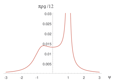
Figure 1: The susy vacuum number density per unit $\psi$ coordinate volume, $\pi\rho g_{\psi\bar{\psi}}/12$, on the real $\psi$-axis, for the mirror quintic.

Fig. 1 shows a plot of $\frac{\pi}{12}\,\rho g_{\psi\bar{\psi}}$, i.e. the susy vacuum number density per unit $\psi$ coordinate volume, on the real $\psi$-axis (the factor $\pi/12$ comes from integrating over $\tau$). The drop for $|\psi|>1$ is due to a similar drop in $g_{\psi\bar{\psi}}$; $\rho$ itself tends to the large complex structure value $2/\pi^{2}$ when $\psi\to\infty$. The divergence at $\psi=1$ is due to the presence of a conifold singularity there. In the notation of example 2, the parameters specifying $g$ and ${\cal F}$ near the conifold are $\mu=8.94$ and $c=1.26\times 10^{-2}$ (with $v\approx-4\pi^{2}5^{-3/2}\,(\psi-1)$).

We numerically computed the integrated susy vacuum number density. We found:

$$\int_{{\cal M}}d\mu=5.46\times 10^{-2}.$$ (88)

This can be compared with an estimate of the large complex structure contribution, obtained similar to Eq. (74) by using the LCS expressions for $g$ and $\rho$, but now cutting off the integral say at $\mbox{Im }t=2$. (Here $t$ defined by $5\psi\equiv e^{-2\pi it/5}$, and the conifold point is located at $\mbox{Im }t|_{\psi=1}=2\pi/5\ln 5=1.28$.) The result is $1/16\pi=1.99\times 10^{-2}$. The exact numerical result for this region is almost the same: $1.97\times 10^{-2}$. Thus for orientifolds of the mirror quintic, about 36% of all susy flux vacua are at $\mbox{Im }t>2$ (and this fraction is proportional to one over the lower bound on $\mbox{Im }t$). On the other hand, using Eq. (86), we get that the fraction of vacua with $|\psi-1|<S\ll 1$ equals $0.486/\ln(6.41/S^{2})$. For $S=10^{-3}$, this is about 3 %, and for $S=10^{-10}$ still 1%.

For the integrated index density, we found

$$\int d\mu_{ind}=-1.666\times 10^{-2}\approx-1/60$$ (89)

Combined with Eq. (82), this indicates that $\chi({\cal M}_{Y})=1/5$. Indeed, this can be verified analytically. The integral of the Euler class can be written as a sum of boundary contour integrals as follows:

$$\chi = \frac{i}{2\pi}\int_{{\cal M}_{Y}}\bar{\partial}\partial\ln g_{\psi\bar{\psi}}$$ (90)

$$= \frac{i}{2\pi\times 5}\int_{\mathbb{C}}\bar{\partial}\partial\ln g_{\psi\bar{\psi}}$$ (91)

$$= \frac{i}{10\pi}\biggl{(}\oint_{\infty}\partial\ln g_{\psi\bar{\psi}}-\sum_{i=1}^{5}\oint_{P_{i}}\partial\ln g_{\psi\bar{\psi}}\biggr{)}$$ (92)

where the $P_{i}$ are the 5 copies of the conifold point in the $\psi$-plane. For $\psi\to\infty$ we have $g_{\psi\bar{\psi}}=3/4|\psi|^{2}\ln^{2}|\psi|$, so

$$\partial\ln g_{\psi\bar{\psi}}=-\frac{1}{\psi}\biggl{(}1+\frac{1}{\ln|\psi|}\biggr{)}d\psi$$ (93)

and the corresponding contour integral produces a contribution $(i/10\pi)\times(-2\pi i)=1/5$ to Eq. (92). On the other hand, near the conifold point $\psi=1$, $g_{\psi\bar{\psi}}=c\ln(\mu^{2}/|\psi-1|^{2})$, and

$$\partial\ln g_{\psi\bar{\psi}}=-\frac{1}{\ln\frac{\hat{\mu}^{2}}{|\psi-1|^{2}}}\frac{1}{\psi-1}\,d\psi,$$ (94)

so the corresponding contour integral is zero. Adding up all contributions, we thus see that $\chi=1/5$.

Numerical integration of the volume of ${\cal M}$ gives $5\mbox{vol}({\cal M})=3.1416\approx\pi$. Again, this can be understood topologically, using

$$\omega=\frac{i}{2}\partial\bar{\partial}{\cal K}=\frac{i}{2}\bar{\partial}\partial\ln i\langle\hat{\Omega},\bar{\hat{\Omega}}\rangle,$$ (95)

plus the fact that if $\hat{\Omega}$ is normalized such that ${\cal K}$ is regular at $\psi=0$, we have $\langle\hat{\Omega},\bar{\hat{\Omega}}\rangle\sim 1/|\psi|^{2}\ln^{3}|\psi|$ for $\psi\to\infty$. Writing the volume integral as a sum over contours, again only the $\psi=\infty$ contour contributes, and this contribution equals $\pi$, as expected.

3.1.6 $d^{2}|W|$ signature distribution

For some applications, such as the RG flow interpretation of domain wall flows, one needs to know whether the critical point of $W$ is a maximum, a minimum, or a saddle point of $|W|$. This corresponds to a positive, negative or indefinite Hessian $d^{2}|W|\equiv(\partial_{a},\bar{\partial}_{\bar{a}})^{t}\cdot(\bar{\partial}_{\bar{b}}|W|,\partial_{b}|W|)$. At a critical point, one has $\partial_{a}\partial_{b}|W|=\frac{1}{2}\frac{\bar{W}}{|W|}D_{a}D_{b}W$ and $\partial_{a}\bar{\partial}_{b}|W|=\frac{1}{2}\frac{W}{|W|}D_{a}\bar{D}_{\bar{b}}\bar{W}$, so from Eq. (59) we see that we have to investigate the eigenvalues of

$$d^{2}|W|=\frac{1}{2|X|}\left(\begin{array}[]{cccc}|X|^{2}&0&0&\bar{X}Z\\ 0&|X|^{2}&\bar{X}Z&{\cal F}\bar{X}\bar{Z}\\ 0&X\bar{Z}&|X|^{2}&0\\ X\bar{Z}&\bar{{\cal F}}XZ&0&|X|^{2}\end{array}\right)$$ (96)

Clearly the sum of the eigenvalues ${\rm tr\,}d^{2}|W|\geq 0$, so there are no maxima (this is true in general, since $\partial_{a}\bar{\partial}_{\bar{b}}|W|\sim g_{a\bar{b}}|W|$ and ${\rm tr\,}g>0$). In general, a matrix is positive definite iff all upper left submatrices have positive determinant. In the case at hand, this implies the conditions $|X|^{4}+|Z|^{4}-(2+|{\cal F}|^{2})|X|^{2}|Z|^{2}>0$ and $|X|^{2}-|Z|^{2}>0$. This restricts the integration domain of Eq. (71) to one of its three segments, and thus the density of susy vacua which are minima of $|W|$ is

$$\rho_{++++}=\frac{1}{2\pi^{2}}(2-|{\cal F}|^{2}+\frac{|{\cal F}|^{3}}{\sqrt{4+|{\cal F}|^{2}}}).$$ (97)

More information can be obtained by looking directly at the eigenvalues. We just quote the results: $\rho_{++--}=\rho_{++++}$, and

$$\rho_{+++-}=\frac{1}{\pi^{2}}\frac{|{\cal F}|^{3}}{\sqrt{4+|{\cal F}|^{2}}}.$$ (98)

In the large complex structure limit one has, rather democratically, $\rho_{++++}=\rho_{+++-}=\rho_{++--}=\rho/3$. In the conifold limit on the other hand, $\rho_{+++-}=\rho$ and $\rho_{++++}=\rho_{++--}=0$.

3.2 Number of susy vacua with positive bosonic mass matrix

Due to the properties of AdS, supersymmetric vacua are always perturbatively stable, even if the critical point of the potential $V$ is not a minimum. Obviously, this is no longer true if supersymmetry is broken and the cosmological constant is lifted to a positive value. In particular, if as in the KKLT scenario supersymmetry is broken by adding an anti-D3 brane to a supersymmetric AdS vacuum, thus shifting the potential up by a constant such that the critical point of the potential becomes positive, the original AdS critical point should be a minimum in order for the lifted vacuum to be perturbatively stable. It is therefore important to compute the number of supersymmetric vacua which are local minima of $V$.

A critical point is a minimum if the mass matrix $d^{2}V\equiv(\partial,\bar{\partial})^{t}\cdot(\bar{\partial}V,\partial V)$ is positive definite. Using Eq. (6)–Eq. (8) and Eq. (35)–Eq. (41), we get, at a supersymmetric critical point (i.e. $Y=0$):

$$D_{0}\partial_{0}V = 0$$ (99)

$$D_{I}\partial_{0}V = -Z_{I}\bar{X}$$ (100)

$$D_{0}\partial_{J}V = -Z_{J}\bar{X}$$ (101)

$$D_{I}\partial_{J}V = -{\cal F}_{IJK}\bar{Z}^{K}\bar{X}$$ (102)

$$D_{0}\bar{\partial}_{0}V = -2|X|^{2}+|Z_{I}|^{2}$$ (103)

$$D_{I}\bar{\partial}_{0}V = {\cal F}_{IKL}\bar{Z}^{K}\bar{Z}^{L}$$ (104)

$$D_{0}\bar{\partial}_{J}V = \bar{{\cal F}}_{JKL}Z^{K}Z^{L}$$ (105)

$$D_{I}\bar{\partial}_{J}V = -2|X|^{2}+Z_{I}\bar{Z}_{J}+{{\cal F}_{IK}}^{M}\bar{{\cal F}}_{MJL}\bar{Z}^{K}Z^{L}$$ (106)

We can use covariant derivatives of $V$ here instead of ordinary derivatives because $dV=0$ implies $DdV=d^{2}V$.

Let us work out the case $n=1$, which has

$$d^{2}V=\left(\begin{array}[]{cccc}|Z|^{2}-2|X|^{2}&\bar{{\cal F}}Z^{2}&0&-\bar{X}Z\\ {\cal F}\bar{Z}^{2}&(1+|{\cal F}|^{2})|Z|^{2}-2|X|^{2}&-\bar{X}Z&-{\cal F}\bar{X}\bar{Z}\\ 0&-X\bar{Z}&|Z|^{2}-2|X|^{2}&{\cal F}\bar{Z}^{2}\\ -X\bar{Z}&-\bar{{\cal F}}XZ&\bar{{\cal F}}Z^{2}&(1+|{\cal F}|^{2})|Z|^{2}-2|X|^{2}\end{array}\right)$$ (107)

A matrix is positive definite iff all its upper left subdeterminants are positive. With $r\equiv|X|^{2}$, $s\equiv|Z|^{2}$, this gives the following conditions:

$$s-2r > 0$$ (108)

$$4\,r^{2}-2\,\left(2+|{\cal F}|^{2}\right)\,r\,s+s^{2} > 0$$ (109)

$$\left(s-2\,r\right)\,\left(4\,r^{2}-\left(5+2\,|{\cal F}|^{2}\right)\,r\,s+s^{2}\right) > 0$$ (110)

$$\left(16\,r^{2}-4\,\left(2+|{\cal F}|^{2}\right)\,r\,s+s^{2}\right)\,\left(r^{2}-\left(2+|{\cal F}|^{2}\right)\,r\,s+s^{2}\right) > 0.$$ (111)

A straightforward analysis of these inequalities shows that they boil down to simply

$$|Z|^{2}/|X|^{2}=s/r>4+2|{\cal F}|^{2}+2|{\cal F}|\sqrt{4+|{\cal F}|^{2}}.$$ (112)

To compute the number density of susy vacua with positive mass matrix, we should therefore evaluate the integral Eq. (71) with $(r,s)$ restricted to the region satisfying this condition. This gives

$$\rho_{M>0}=\frac{98+179\,|{\cal F}|^{2}+42\,|{\cal F}|^{4}+96\,|{\cal F}|\,{\sqrt{4+|{\cal F}|^{2}}}+42\,|{\cal F}|^{3}\,{\sqrt{4+|{\cal F}|^{2}}}}{{\left(5+2\,|{\cal F}|^{2}+2\,|{\cal F}|\,{\sqrt{4+|{\cal F}|^{2}}}\right)}^{3}\,{\pi}^{2}}$$ (113)

as shown in fig. 2. At ${\cal F}=0$, the relative fraction of susy vacua with positive mass matrix is approximately 39% and maximal. In the large complex structure limit ${\cal F}=2/\sqrt{3}$ the fraction is about 19%, and in the conifold limit it is zero. Indeed, while the total density $\rho$ grows quadratically with $|{\cal F}|$ when ${\cal F}\to\infty$, the density $\rho_{M>0}$ decreases quadratically with $|{\cal F}|$. This means that very near a conifold point, though there are many susy vacua, only an extremely small fraction has positive mass matrix!

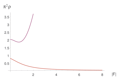
Figure 2: The upper curve shows the total susy vacuum density as a function of $|{\cal F}|$, the lower curve the density of susy vacua with positive mass matrix.

Let us make this more precise. In the notation of our example 2 in the previous section, we have for small $v$:

$$\rho_{M>0}\approx\frac{21\,c^{2}}{6\pi^{2}}\biggl{(}\ln\frac{\mu^{2}}{|v|^{2}}\biggr{)}^{4}\,|v|^{2}.$$ (114)

Integrated over $\tau$ and $|v|<R$, this gives

$$\int d^{2}\tau g_{\tau\bar{\tau}}\int d^{2}v\,g_{v\bar{v}}\,\rho_{M>0}=\frac{7c^{2}}{256}(3+6\gamma+6\gamma^{2}+4\gamma^{3}+2\gamma^{4})R^{4},$$ (115)

where $\gamma(R)=\ln\frac{\mu^{2}}{R^{2}}$. Because of the $R^{4}$ dependence, this rapidly goes to zero with $R$. If we take the parameters of the mirror quintic conifold for example, i.e. $\mu=8.94$ and $c=1.26\times 10^{-2}$, and we take $L_{*}=100$, then the expected number of susy vacua with $M>0$ drops below 1 for $|v|<0.02$, or $|\psi-1|<0.004$. Increasing $L_{*}$ to 1000, these numbers become just one order of magnitude smaller. Thus, for $n=1$ and with reasonable parameter values, at most only a modest hierarchy of scales can be generated through the conifold throat mechanism of [22], if we insist on having a positive mass matrix.

On the other hand, if a near-conifold vacuum has positive mass matrix, Eq. (112) together with $|X|^{2}+|Z|^{2}=L\leq L_{*}$ shows that it automatically has a small value for $|W|=|X|$, and therefore a small cosmological constant. We will make this more precise in the next section.

The positivity properties of $M=d^{2}V$ for susy vacua can also be analyzed as follows. First observe that in general, if $DW=0$,

$$M=H^{2}-3|W|H,$$ (116)

where

$$H=2\,d^{2}|W|.$$ (117)

This follows directly from Eq. (7)–Eq. (8). Thus, to have $M>0$, all eigenvalues $\lambda$ of $H$ must satisfy $\lambda<0$ or $\lambda>3|W|$. In particular, if $W=0$ at the critical point, $M$ is automatically non-negative, and by continuity the same will be true for most susy vacua with small $W$. The suppression of vacua with $M>0$ near a conifold point (for $n=1$) can now be seen in the following way. According to Eq. (96), the matrix $H$ can be written as $H=|X|\,{\bf 1}+\Delta H$, with

$$\Delta H=\left(\begin{array}[]{cc}0&S\\ \bar{S}&0\end{array}\right),\qquad S=\frac{\bar{X}}{|X|}\left(\begin{array}[]{cc}0&Z\\ Z&{\cal F}\bar{Z}.\end{array}\right)$$ (118)

The eigenvalues of $\Delta H$ are $(\pm\lambda_{1},\pm\lambda_{2})$, with $\lambda_{1}^{2}\lambda_{2}^{2}=\det\Delta H=|Z|^{4}$ and $2(\lambda_{1}^{2}+\lambda_{2}^{2})={\rm tr\,}(\Delta H)^{2}=2(|{\cal F}|^{2}+2)|Z|^{2}$. When ${\cal F}\to\infty$, the eigenvalues of $\Delta H$ are therefore approximately given by $\pm|{\cal F}|^{\pm 1}|Z|$, and the eigenvalues of $H$ by $\lambda=|X|\pm|{\cal F}|^{\pm 1}|Z|$. The condition on $\lambda$ to have $M>0$ translates to $|Z|>2|{\cal F}||X|$, in agreement with what we found earlier.

Note that the “dangerous” eigenvectors (the eigenvectors of $\Delta H$ with eigenvalues $\sim 1/|{\cal F}|$) are approximately aligned with the dilaton direction, i.e. $(1,O[1/{\cal F}],1,O[1/{\cal F}])$. In a sense, the special form of the matrix Eq. (118) leads to a sort of “seesaw” mixing with the dilaton, and the small eigenvalue. This may be specific to $n=1$; a similar analysis for $n>1$ suugests that there is no longer suppression of $M>0$ vacua near generic points of the discriminant locus.

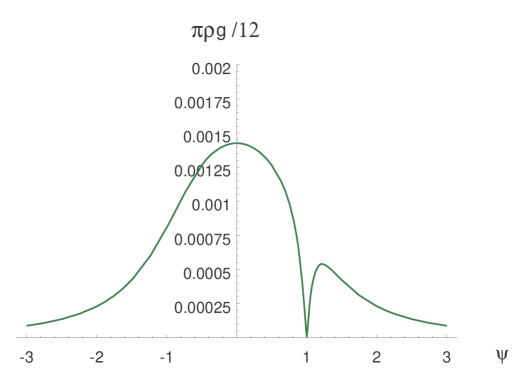
Figure 3: The number density of susy vacua with positive mass matrix, per unit coordinate volume, on the real $\psi$-axis, for the mirror quintic. Compare to fig. 1.

As an example, a plot of the number density of $M>0$ vacua per unit coordinate volume is shown in fig. 3 for the mirror quintic, on the real $\psi$-axis. The sharp dip near $\psi=1$ is due to the conifold singularity. For the integrated density we find

$$\int_{{\cal M}}d\mu_{M>0}=5.12\times 10^{-3}.$$ (119)

Comparing this to Eq. (88), we thus see that about 9% of all susy vacua has positive mass matrix. This is not too far from the naive guess $1/16$ based on the fact that there are four mass eigenvalues, with each a 50% chance to be positive.

3.3 Distribution of cosmological constants

The cosmological constant in a supersymmetric vacuum is $V=-3|W|^{2}$ (in $2T_{3}\equiv 1$ units). We wish to count the number of susy vacua with $L\leq L_{*}$ and $V\geq V_{*}\equiv-3\lambda_{*}$, i.e. with $|W|^{2}\leq\lambda_{*}$. Analogous to Eq. (45), we have

$${\cal N}_{susy}(L\leq L_{*},|W|^{2}\leq\lambda_{*})=\int_{{\cal M}}d^{2m}\!z\int_{0}^{\lambda_{*}}\!d\lambda\,\frac{1}{2\pi i}\int\frac{d\alpha}{\alpha}e^{\alpha L_{*}}\nu(z,\alpha,\lambda)$$ (120)

where

$$\nu(z,\alpha,\lambda) = \int d^{K}\!N\,e^{-\alpha L}\,\delta(|W|^{2}-\lambda)\,\delta^{2m}(DW)\,|\det D^{2}W|$$ (121)

$$= \alpha^{1-K/2}\int d^{K}\!N\,e^{-L}\,\delta(|W|^{2}-\alpha\lambda)\,\delta^{2m}(DW)\,|\det D^{2}W|.$$ (122)

Parallel to Eq. (68), we can write Eq. (120) also in the form

$${\cal N}_{susy}(L\leq L_{*},|W|^{2}\leq\lambda_{*})=\frac{(2\pi L_{*})^{K/2}}{(K/2)!}|\det\eta|^{-1/2}\int_{{\cal M}}d^{2m}\!z\,g\int_{0}^{\lambda_{*}}\!d\lambda\,\rho(\lambda,z)$$ (123)

The quantity $d\lambda\,\rho(\lambda,z)/\rho(z)$ then gives the fraction of vacua at $z$ with $|W|^{2}$ in a width $d\lambda$ interval around $\lambda$.

Specializing again to the orientifold limit, so $K=4m=4(n+1)$, we make the change of variables from $N$ to $(X,Y,Z)$. In these variables the additional constraint in Eq. (122) is simply $|X|^{2}=\alpha\lambda$, which we can solve by putting $X=\sqrt{\alpha\lambda}$, since the integral is invariant under an overall phase transformation of $(X,Y,Z)$. Thus we find, similar to Eq. (69) (but with the additional constraint):

$$\nu(z,\alpha,\lambda) = \frac{2^{2m}\pi g}{\sqrt{\eta}\,\alpha^{2m-1}}\int d^{2n}\!Z\,e^{-\alpha\lambda-|Z|^{2}}\,|\det\left(\begin{array}[]{cccc}\sqrt{\alpha\lambda}&0&0&Z_{J}\\ 0&\delta_{IJ}\sqrt{\alpha\lambda}&Z_{I}&{\cal F}_{IJK}\bar{Z}^{K}\\ 0&\bar{Z}_{J}&\sqrt{\alpha\lambda}&0\\ \bar{Z}_{I}&\bar{{\cal F}}_{IJK}Z^{K}&0&\delta_{IJ}\sqrt{\alpha\lambda}\end{array}\right)\!|$$ (128)

$$= \frac{2^{2m}\pi g}{\sqrt{\eta}\,\alpha^{2m-1}}\,e^{-\alpha\lambda}\int d^{2n}\!Z\,e^{-|Z|^{2}}|\sum_{k=0}^{m}C_{k}(Z,\bar{Z})(\alpha\lambda)^{k}|$$ (129)

where $g\equiv\det g$, $\eta=|\det\eta|$ and the $C_{k}(Z,\bar{Z})$ are homogeneous polynomial functions obtained by expanding the determinant. For example in the $n=1$ case,

$$\nu(z,\alpha,\lambda)=\frac{16\pi g}{\sqrt{\eta}\,\alpha^{3}}\,e^{-\alpha\lambda}\int d^{2}\!Z\,e^{-|Z|^{2}}\,|(\alpha\lambda)^{2}-(2+|{\cal F}|^{2})|Z|^{2}\alpha\lambda+|Z|^{4}|.$$ (130)

3.3.1 Density at zero cosmological constant

For physical applications, the most interesting quantity is the number of vacua at very small cosmological constant, i.e. the case $\lambda_{*}\ll L_{*}$. To a good approximation, we can then neglect the higher order terms in Eq. (129) and simply compute the density at $\lambda=0$. The integral becomes

$$I({\cal F})=\int d^{2n}\!Z\,e^{-|Z|^{2}}|\det\left(\begin{array}[]{cc}0&Z_{J}\\ Z_{I}&{\cal F}_{IJK}\bar{Z}^{K}\end{array}\right)|^{2}.$$ (131)

This is a significant simplification compared to Eq. (129), as this can be evaluated using Wick’s theorem or by rewriting the determinant as a Grassmann integral and then doing the integral over $Z$, similar to what was done to obtain Eq. (76). Doing the integral over $\alpha$ in Eq. (120) now gives

$$\rho|_{\lambda=0}=\frac{2\pi m}{\pi^{2m}L_{*}}I({\cal F})$$ (132)

Note that for $n=1$, this is independent of ${\cal F}$ and therefore of $z$: $\rho_{0}=8/\pi^{2}L_{*}$. Applying this to the example of the mirror quintic, for which $\mbox{vol}({\cal M}_{\tau}\times{\cal M}_{\psi})=\frac{\pi}{12}\times\frac{\pi}{5}$, we get for small $\lambda_{*}$:

$${\cal N}(L\leq L_{*},|W|^{2}\leq\lambda_{*})=\frac{4\pi^{4}L_{*}^{4}}{45}\,\frac{\lambda_{*}}{L_{*}}$$ (133)

For $L_{*}=100$, this becomes $\sim 10^{7}\lambda_{*}$, so the expected smallest possible cosmological constant is $|\Lambda|\sim 10^{-7}T_{3}$. For $L_{*}=1000$, this is three orders of magnitude smaller.

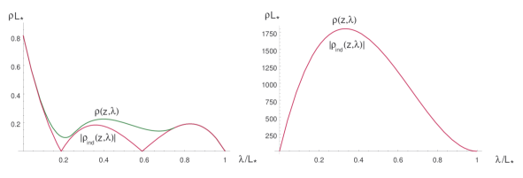
Figure 4: Left: Vacuum number densities (true and absolute value of index) in the large complex structure limit (${\cal F}=2/\sqrt{3}$), as a function of cosmological constant value. Right: Same near the conifold limit (${\cal F}=100$ for this example). Note that despite appearances, $\rho$ is non-zero at $\lambda=0$ as expressed in Eq. (133); it just does not receive the conifold enhancement there.

3.3.2 Index density

The distribution for arbitrary cosmological constants is harder to compute, mainly because of the absolute value signs in Eq. (129). Let us therefore drop these for now, so we count vacua with signs. Then after integration over $Z$, we will still have a polynomial in $\alpha$:

$$\nu_{ind}(z,\alpha,\lambda)=\frac{2^{2m}\pi^{m}g}{\sqrt{\eta}}\,e^{-\alpha\lambda}\sum_{k=0}^{m}c_{k}\lambda^{k}\alpha^{k-2m+1}$$ (134)

and therefore, by comparing Eq. (120) and Eq. (123),

$$\rho_{ind}(z,\lambda) = \frac{(2m)!}{(2\pi L_{*})^{2m}g}\frac{1}{2\pi i}\int\frac{d\alpha}{\alpha}e^{\alpha L_{*}}\nu_{ind}(z,\alpha,\lambda)$$ (135)

$$= \theta(L_{*}-\lambda)\frac{(2m)!}{\pi^{m}L_{*}}\sum_{k=0}^{m}\frac{c_{k}}{(2m-1-k)!}\left(\frac{\lambda}{L_{*}}\right)^{k}\left(1-\frac{\lambda}{L_{*}}\right)^{2m-1-k}$$ (136)

In the case $n=1$, we thus get for the cosmological constant density counted with signs

$$\rho_{ind}(z,\lambda)=\frac{4}{L_{*}\pi^{2}}(1-x)(2-(10+3|{\cal F}|^{2})\,x+(14+3|{\cal F}|^{2})\,x^{2})\,\theta(1-x)$$ (137)

where we wrote $x\equiv\frac{\lambda}{L_{*}}$. As noted above, the density at $\lambda=0$ equals $8/L_{*}\pi^{2}$. In the large complex structure limit ${\cal F}\to 2/\sqrt{3}$, $\rho_{ind}=8(1-x)(1-7x+9x^{2})/L_{*}\pi^{2}$ and in the conifold limit ${\cal F}\to\infty$, for $x$ not too small, $\rho_{ind}/|{\cal F}|^{2}=-12(1-x)^{2}x/L_{*}\pi^{2}$.

3.3.3 Total density

Let us now turn to the true density. The absolute value signs in Eq. (129) make the integral hard to evaluate in general, but for $n=1$ one gets something of the form

$$\nu(z,\alpha,\lambda)=P_{0}(\alpha\lambda)e^{-\alpha\lambda}+P_{-}(\alpha\lambda)e^{-b_{-}\alpha\lambda}+P_{+}(\alpha\lambda)e^{-b_{+}\alpha\lambda}$$ (138)

with the $P_{i}$ polynomials and $b_{-}$, $b_{+}$ some ${\cal F}$-dependent coefficients (see below). Doing the $\alpha$-contour integral, this then gives, explicitly:

$$L_{*}\pi^{2}\,\rho(z,\lambda)=L_{*}\pi^{2}\rho_{ind}(z,\lambda)+P(x)(\theta(1-b_{-}x)-\theta(1-b_{+}x))+Q(x)(\theta(1-b_{-}x)+\theta(1-b_{+}x))$$ (139)

where

$$P(x) = -4+6(4+|{\cal F}|^{2})\,x-12(4+|{\cal F}|^{2})\,x^{2}+(32-6|{\cal F}|^{4}-|{\cal F}|^{6})\,x^{3}$$ (140)

$$Q(x) = (4+|{\cal F}|^{2})^{3/2}F^{3}x^{3}$$ (141)

$$b_{\pm} = \frac{1}{2}\sqrt{4+|{\cal F}|^{2}}(\sqrt{4+|{\cal F}|^{2}}\pm|{\cal F}|)$$ (142)

In the large complex structure limit

$$L_{*}\pi^{2}\rho(z,\lambda)=L_{*}\pi^{2}\rho_{ind}(z,\lambda)+16(1-4x)^{2}\,\theta(1-4x)+\frac{16}{27}(16x-3)(3-4x)^{2}\,\theta(3-4x),$$ (143)

and in the conifold limit, for $x$ not too small,

$$\rho(z,\lambda)/|{\cal F}|^{2}\to 12(1-x)^{2}x/L_{*}\pi^{2}=-\rho_{ind}(\lambda,z).$$ (144)

This is not immediately obvious from the above expressions, but can be seen from Eq. (130): the middle term dominates, and the absolute value just removes the minus sign. As discussed before, the convergence of index density and true density can be expected to hold more generally near degenerations where ${\cal F}_{IJK}\to\infty$ (see also below).

These considerations are illustrated for the large complex structure and conifold limits in fig. 4. Note that the approximation of the true density by the index density is perfect near the conifold, and near the extremities of $\lambda$, and qualitatively still not bad away from those.

3.3.4 Some general observations

A few simple observations can be made about the general case. It is obvious that the cosmological constant always satisfies $|W|^{2}<L_{*}$. This is because $|W|^{2}+|Z|^{2}=L\leq L_{*}$ by construction. The density at $\lambda=L_{*}$ is zero for the same reason; in fact, the index density near that point is suppressed by $(L-\lambda_{*})^{m-1}$, as follows from Eq. (135). By contrast, the density at $\lambda=0$ is always nonvanishing. Note however that in case all ${\cal F}_{IJK}\to\infty$, this value is much smaller than the total density $\rho(z)$ (compare Eq. (131) to Eq. (75)). In general, for large $m$, the distribution can be expected to peak at a small value of $\lambda$, because of the suppression factor $(L-\lambda_{*})^{m-1}$. More intuitively, the lower $|W|^{2}$ is, the more “room” there is for $Z$ to satisfy $|W|^{2}+|Z|^{2}\leq L_{*}$.

Finally, in the limit where ${\cal F}_{IJK}\to\infty$, we can compute $\rho(z,\lambda)$ more explicitly, since then, for $\lambda$ not too small,

$$\rho(z,\lambda) \approx \frac{(2m)!}{(\pi L_{*})^{2m}}\frac{1}{2\pi i}\int\frac{d\alpha}{\alpha}e^{\alpha L_{*}}\frac{\pi}{\alpha^{2m-1}}\int d^{2n}\!Z\,e^{-\alpha\lambda-|Z|^{2}}\,\alpha\lambda|\det({\cal F}_{IJK}\bar{Z}^{K})|^{2}$$ (145)

$$= A\,x\,(1-x)^{2m-2}$$ (146)

where $x=\lambda/L_{*}$, and $A=\frac{2m(2m-1)}{\pi^{2m-1}L_{*}}\int d^{2n}\!Z\,e^{-|Z|^{2}}\,|\det({\cal F}_{IJK}\bar{Z}^{K})|^{2}$. This distribution has mean $\mu=\langle x\rangle=2/(2m+1)$ and standard deviation $\sigma^{2}=\langle(x-\mu)^{2}\rangle=(2m-1)/(m+1)(2m+1)^{2}$, so for large $m$, most susy vacua in this limit have a cosmological constant $\Lambda$ of order $-T_{3}L_{*}/m$. This should be compared to the string scale energy density, which in Einstein frame is $T_{F}^{2}=g_{s}(2\pi\alpha^{\prime})^{-2}=2\pi g_{s}T_{3}$. Therefore in this limit vacua with $|\Lambda|$ well below the string scale are comparatively rare, unless $m\gg L_{*}/g_{s}$.

3.3.5 Distribution restricted to vacua with positive mass matrix

If we restrict to vacua with positive mass matrix, Eq. (112) together with $|Z|^{2}+|X|^{2}=L\leq L_{*}$, implies the cutoff $\lambda\leq L_{*}/(5+2|{\cal F}|^{2}+2|{\cal F}|\sqrt{4+|{\cal F}|^{2}})$. In the large complex structure limit, this is $\lambda\leq L_{*}/13$, and near the conifold limit, $\lambda\leq L_{*}/4|{\cal F}|^{2}$. Therefore, positive $M$ vacua near the conifold point automatically have small cosmological constant (small compared to the string scale). Recall however that positive $M$ vacua are suppressed near the conifold point. We saw earlier that for the parameter values of the mirror quintic and $L_{*}=100$, no positive $M$ vacua are expected below $v\sim 10^{-2}$. At this point ${\cal F}\sim 20$ and thus $\lambda<10^{-3}L_{*}=0.1$, hence the cosmological constant cutoff is not much below the string scale. Increasing $L_{*}$ to 1000 decreases the $\lambda$ cutoff with just one order of magnitude. Thus, for $n=1$, the positive $M$ vacua closest to the conifold point are not expected to be close enough to force the cosmological constant to be hierarchically smaller than the string scale.

This does not mean of course that there are no $M>0$ vacua with very small cosmological constant; in fact, the vacuum density at $\lambda_{*}=0$ is the same for $M>0$-vacua as for vacua without constraints on $M$, since if $X=0$, the $M>0$ condition Eq. (112) is automatically satisfied. Most vacua with very small $\lambda$ will therefore have a positive mass matrix. This is actually true for any supergravity theory, as follows from Eq. (9).

3.4 Counting attractor points

The techniques we used to count supersymmetric flux vacua can also be used to count supersymmetric black holes, or attractor points, in type IIB theory compactified on a Calabi-Yau $X$. More precisely, we wish to count the number of duality inequivalent, regular, spherically symmetric, BPS black holes with entropy $S$ less than $S_{*}$. The charge of a black hole is given by an element $Q=N^{\alpha}\Sigma_{\alpha}$ of $H^{3}(X,\mathbb{Z})$. The central charge ${\cal Z}=\langle Q,\Omega_{3}\rangle$ plays a role similar to the (normalized) superpotential $W$: the moduli at the horizon are always fixed at a critical point of $|{\cal Z}|$, i.e. $D{\cal Z}=(\partial+\partial{\cal K}){\cal Z}=0$. The entropy is then given by $S=A/4=\pi|{\cal Z}|^{2}$, evaluated at the critical point. For a given $Q$, critical points may or may not exist, may or may not be located in the fundamental domain ${\cal M}$, and may or may not be unique, but clearly we can label all equivalence classes of black holes by a charge vector $N$ and a critical point within the fundamental domain. Thus our desired number is, in a continuum approximation (valid for large $S_{*}$) similar to what we had before:

$${\cal N}_{BH}(S\leq S_{*})=\frac{1}{2\pi i}\int\frac{d\alpha}{\alpha}\,e^{\alpha S_{*}/\pi}\int d^{K}\!N\int_{{\cal M}}d^{2n}\!z\,e^{-\alpha|{\cal Z}|^{2}}\,\delta^{2n}(D{\cal Z})\,|\det D^{2}{\cal Z}|.$$ (147)

Here $K$ is the number of flux components and $n$ the number of complex structure moduli, $K=2n+2$. After rescaling $N\to N/\sqrt{\alpha}$, doing the $\alpha$ integral becomes straightforward, and we get

$${\cal N}_{BH}(S\leq S_{*})=\frac{(2S_{*})^{n+1}}{(n+1)!}\int_{{\cal M}}d^{2n}\!z\,\det g\,\rho(z)$$ (148)

where

$$\rho(z)=\frac{1}{(2\pi)^{n+1}\det g}\int d^{2n+2}\!N\,e^{-|{\cal Z}|^{2}}\delta^{2n}(D{\cal Z})\,|\det D^{2}{\cal Z}|.$$ (149)

To evaluate this integral, we change variables to a Hodge-decomposition basis of $H^{3}(X)$, similar to Eq. (34):

$$Q=i\bar{X}\Omega-i\bar{Y}^{I}D_{I}\Omega+c.c.,$$ (150)

so ${\cal Z}=\langle Q,\Omega\rangle=X$ and $D_{I}{\cal Z}=\langle Q,D_{I}{\cal Z}\rangle=Y_{I}$. Capital indices again refer to an orthonormal frame. The Jacobian for the change of variables from $N$ to $(X,Y,\bar{X},\bar{Y})$ can be computed in a way analogous to what we did for flux vacua; the result is $J=2^{n+1}|\eta|^{-1/2}$, where $|\eta|$ is the determinant of the intersection form (equal to 1 if we sum over the full charge lattice). Furthermore, using the special geometry identity $D_{I}D_{J}{\cal Z}={\cal F}_{IJK}Y^{K}$, we get that at a critical point (where $Y=0$):

$$\det\left(\begin{array}[]{cc}D_{I}\bar{D}_{J}\bar{{\cal Z}}&D_{I}D_{J}{\cal Z}\\ \bar{D}_{I}\bar{D}_{J}\bar{{\cal Z}}&\bar{D}_{I}D_{J}{\cal Z}\end{array}\right)=\det\left(\begin{array}[]{cc}\delta_{IJ}\bar{X}&0\\ 0&\delta_{IJ}X\end{array}\right)=|X|^{2n}.$$ (151)

Plugging this in Eq. (149) gives

$$\rho = \frac{1}{\pi^{n}|\eta|^{1/2}}\int d^{2}\!X\int d^{2n}\!Y\,e^{-|X|^{2}}\,\delta^{2n}(Y)\,|X|^{2n}$$ (152)

$$= \frac{n!}{\pi^{n}|\eta|^{1/2}}.$$ (153)

The factor $\det g$ dropped out because of the change from coordinate to orthonormal frame. Note that this expression for $\rho$ is independent of $z$. This means that attractor points are uniformly distributed over moduli space. Our final result is, for large $S_{*}$:

$${\cal N}_{BH}(S\leq S_{*})=\frac{2^{n+1}\,\mbox{vol}({\cal M})}{(n+1)\,\pi^{n}\,|\eta|^{1/2}}\,{S_{*}}^{n+1}.$$ (154)

For the mirror quintic, $n=1$ and $\mbox{vol}({\cal M})=\pi/5$, hence

$${\cal N}_{BH}(S\leq S_{*})=\frac{2}{5}{S_{*}}^{2}$$ (155)

The problem of counting the number of duality inequivalent black holes with given entropy was studied in [30] using number theory techniques. In particular, for $Y=T^{2}\times K3$, this was shown to be related to class numbers and the number of inequivalent embeddings of a given two-dimensional lattice into the charge lattice.

To compare to our results, we restrict to algebraic K3’s, as the complex structure moduli moduli space of a generic K3 is not Hausdorff, so the volume factor in Eq. (154) would not make any sense. An algebraic K3 has moduli space

$${\cal M}_{K3}=O(\Lambda)\setminus O(2,k)/O(2)\times O(k),$$

where $\Lambda$ is the charge lattice, which is the orthogonal complement of the Picard lattice and has signature $(2,k)$. This space is Hausdorff and has complex dimension $k$. A black hole charge is specified by two charge vectors $p,q\in\Lambda$.

In this case, counting black holes with given entropy, or more precisely with given “discriminant” $D=(S/\pi)^{2}$ (which is always an integer for $K3\times T^{2}$), amounts roughly to computing the number of inequivalent lattice embeddings in $\Lambda$ of lattices spanned by $q$ and $p$ with determinant $D$. This number can in principle be obtained from the Smith-Minkowski “mass formula”, which was used in [30] to derive an estimate for the asymptotic growth of the number $N(D)$ of inequivalent black holes with discriminant $D$. The result is $N(D)\sim D^{k/2}$ and consequently the number of black holes with $D\leq D_{*}$ will grow as $D_{*}^{1+k/2}$.

To compare with Eq. (154), note that $n=k+1$, so we get

$${\cal N}_{BH}(D\leq D_{*})=\frac{2^{k+2}\pi}{k+2}\mbox{vol}({\cal M}_{T^{2}})\mbox{vol}({\cal M}_{K3})\,D_{*}^{1+k/2},$$ (156)

which agrees with the growth given above, but is a bit more precise. Turning things around, this formula should give a predicition for the asymptotic behavior of the Smith-Minkowski mass formula.

4 Distributions of nonsupersymmetric vacua

A general flux vacuum, supersymmetric or not, is characterized by a flux vector and a critical point of the corresponding potential $V$, which for now we do not require to be a local minimum. For nonsupersymmetric vacua, the condition $L\leq L_{*}$ is no longer sufficient to guarantee a finite volume of allowed fluxes. Physically, it is reasonable to put also a bound on the supersymmetry breaking parameter: $|DW|=|Y|\leq F_{*}$. Such a bound, together with the bound on $L=|X|^{2}-|Y|^{2}+|Z|^{2}$, is indeed precisely what we need to make the volume of allowed fluxes finite.

In our approximation, the total number of flux vacua satisfying these bounds is then given by

$${\cal N}(L\leq L_{*},|DW|\leq F_{*})=2^{2m}\int d^{2m}\!z\int d^{2}\!Xd^{2m}\!Yd^{2n}\!Z\,\theta(L_{*}-L)\,\theta(F_{*}-|Y|)\,\delta^{2m}(dV)\,|\det d^{2}V|$$ (157)

where $d^{2}V=(\partial,\bar{\partial})^{t}\cdot(\bar{\partial}V,\partial V)$, and using Eq. (6)–Eq. (8) and Eq. (35)–Eq. (41):

$$\partial_{0}V = Z_{I}\bar{Y}^{I}-2Y_{0}\bar{X}$$ (158)

$$\partial_{I}V = Z_{I}\bar{Y}^{0}+{\cal F}_{IJK}\bar{Y}^{J}\bar{Z}^{K}-2Y_{I}\bar{X}$$ (159)

$$D_{0}\partial_{0}V = 0$$ (160)

$$D_{I}\partial_{0}V = {\cal F}_{IKL}\bar{Y}^{K}\bar{Y}^{L}-Z_{I}\bar{X}$$ (161)

$$D_{0}\partial_{J}V = {\cal F}_{JKL}\bar{Y}^{K}\bar{Y}^{L}-Z_{J}\bar{X}$$ (162)

$$D_{I}\partial_{J}V = 2{\cal F}_{IJK}\bar{Y}^{0}\bar{Y}^{K}-{\cal F}_{IJK}\bar{Z}^{K}\bar{X}+D_{I}{\cal F}_{JKL}\bar{Z}^{L}\bar{Y}^{K}$$ (163)

$$D_{0}\bar{\partial}_{0}V = -2|X|^{2}-2|Y_{0}|^{2}+|Y_{I}|^{2}+|Z_{I}|^{2}$$ (164)

$$D_{I}\bar{\partial}_{0}V = -Y_{I}\bar{Y}_{0}+{\cal F}_{IKL}\bar{Z}^{K}\bar{Z}^{L}$$ (165)

$$D_{0}\bar{\partial}_{J}V = -Y_{0}\bar{Y}_{J}+\bar{{\cal F}}_{JKL}Z^{K}Z^{L}$$ (166)

$$D_{I}\bar{\partial}_{J}V = -2|X|^{2}+|Y_{0}|^{2}-2Y_{I}\bar{Y}_{J}+Z_{I}\bar{Z}_{J}+{{\cal F}_{IK}}^{M}\bar{{\cal F}}_{MJL}(\bar{Y}^{K}Y^{L}+\bar{Z}^{K}Z^{L})$$ (167)

We can use covariant derivatives of $V$ in the integral instead of ordinary derivatives because if $dV=0$, then $DdV=d^{2}V$.

4.1 Supersymmetric and anti-supersymmetric branches

The main complication arises because the constraint $dV=0$ is quadratic. It defines a cone in $\mathbb{C}^{m}$, which has several branches. One obvious branch is $Y_{A}=0$, with $X$ and $Z_{I}$ arbitrary. This corresponds to the supersymmetric vacua discussed in the previous sections. Another obvious one is $X=Z_{I}=0$. As we will see, the vacua on this branch behave in a way as “anti-supersymmetric” vacua. For example, while susy vacua have imaginary self-dual fluxes, these have imaginary anti-self-dual fluxes. There are more complicated “intermediate” branches too, which arise when the constraints considered as linear equations in $(X,Z)$ (or in $Y$) are degenerate.

On the supersymmetric branch, we have $\delta^{2m}(dV)=|\det M|^{-1}\delta^{2m}(Y)$, with $M=(\partial_{Y},\bar{\partial}_{\bar{Y}})^{t}\cdot(\partial V,\bar{\partial}V)$. This threatens to make the integral divergent when $\det M\to 0$, but note that by the chain rule and because $Y=0$, $d^{2}V|_{Y=0}=(\partial,\bar{\partial})^{t}\cdot(\bar{\partial}V,\partial V)=(\partial,\bar{\partial})^{t}\cdot(\bar{Y},Y)\cdot(\bar{\partial}_{\bar{Y}},\partial_{Y})^{t}\cdot(\bar{\partial}V,\partial V)=D^{2}W\cdot\bar{M}$, so the factor $\det M$ cancels out of Eq. (157) and we are left with the integral we had before for the supersymmetric case, as we should of course.

Similarly, on the branch $X=Z=0$, we have $\delta^{2m}(dV)=|\det M|^{-1}\delta^{2m}(X,Z)$, with $M=(\partial_{X},\partial_{Z},\bar{\partial}_{\bar{X}},\bar{\partial}_{\bar{Z}})^{t}\cdot(\partial V,\bar{\partial}V)$. Again $\det M$ cancels out, because $d^{2}V|_{X=Z=0}=A\cdot\bar{M}$, with

$$A = (D_{0},D_{I},\bar{D}_{0},\bar{D}_{I})^{t}\cdot(\bar{W},\bar{D}_{0}\bar{D}_{J}\bar{W},W,D_{0}D_{J}W)$$ (168)

$$= \left(\begin{array}[]{cccc}0&\bar{Y}_{J}&Y_{0}&0\\ 0&\delta_{IJ}\bar{Y}_{0}&Y_{I}&{\cal F}_{IJK}\bar{Y}^{K}\\ \bar{Y}_{0}&0&0&Y_{J}\\ \bar{Y}_{I}&{\cal F}_{IJK}Y^{K}&0&\delta_{IJ}Y_{0}\end{array}\right),$$ (173)

so the remaining determinant factor in Eq. (157) is

$$\det A=|Y_{0}|^{2}\det\left(\begin{array}[]{cc}\delta_{IJ}\bar{Y}_{0}-\frac{Y_{I}\bar{Y}_{J}}{Y_{0}}&{\cal F}_{IJK}\bar{Y}^{K}\\ \bar{{\cal F}}_{IJK}Y^{K}&\delta_{IJ}Y_{0}-\frac{\bar{Y}_{I}Y_{J}}{\bar{Y}_{0}}\end{array}\right),$$ (174)

which is identical to the $\det D^{2}W$ factor Eq. (67) of the supersymmetric case, after substitution $X\to Y_{0}$, $Z_{I}\to Y_{I}$. If we moreover replace the supersymmetric constraint $L=|X|^{2}+|Z|^{2}\leq L_{*}$ by $|Y|^{2}\leq L_{*}$ (or, since now $L=-|Y|^{2}$, by $L\geq-L_{*}$), the integral for this nonsupersymmetric branch is therefore formally the same as the one for the supersymmetric branch! Thus

$${\cal N}_{X=Z=0}(|DW|\leq F_{*})={\cal N}_{susy}(L\leq F_{*}^{2}).$$ (175)

In fact this can be understood directly from the defining equations. If $(F_{3},H_{3},\tau,z^{i})$ with $\mbox{Im }\tau>0$ solves $F_{3}-\tau H_{3}=i*(F_{3}-\tau H_{3})$, which is the condition for a supersymmetric vacuum, then $(F^{\prime}_{3},H^{\prime}_{3},\tau^{\prime},z^{\prime i})=(-F_{3},H_{3},-\bar{\tau},z^{i})$ has $\mbox{Im }\tau^{\prime}>0$ and solves $F^{\prime}_{3}-\tau^{\prime}H^{\prime}_{3}=-i*(F^{\prime}_{3}-\tau^{\prime}H^{\prime}_{3})$, which is the condition for a nonsupersymmetric vacuum on the branch under consideration. An equivalent way to see this map is to observe that $D_{0}(N_{RR}+\tau N_{NS})\sim-N_{RR}-\bar{\tau}N_{NS}$ together with the fact that the action of $D_{0}$ and $\bar{D}_{0}$ interchanges $(X,Z)$ and $Y$. Note however that this is not a map between vacua with the same topological data, since it maps $L\to-L$; the susy vacua have positive and the nonsusy vacua negative $L$.

The cosmological constant of these nonsupersymmetric vacua is $\Lambda=2T_{3}|DW|^{2}=-2L\,T_{3}$. Since $L$ is quantized, this is always at least of the order of the string scale energy density $T_{F}^{2}=2\pi g_{s}T_{3}$, so actually the field theory approximation on which this analysis is based cannot be trusted, and the existence of these vacua in the full theory is doubtful.

4.2 Intermediate branches

The anti-supersymmetric branch $X=Z=0$ of the constraint cone $dV=0$ is parametrized by the values of the F-terms $Y_{A}$. For generic values of the $Y_{A}$, the unique solution to $dV=0$ is indeed $X=Z=0$, since it is just a generic, complete system of linear equations in $(X,Z)$. However, for some values of $Y$ the linear system can become degenerate, namely when $\det M=0$ where $M$ is as before given by $M=(\partial_{X},\partial_{Z},\bar{\partial}_{\bar{X}},\bar{\partial}_{\bar{Z}})^{t}\cdot(\partial V,\bar{\partial}V)$. This happens at the intersection with other branches.

We will only analyze the case $n=1$ here. Then

$$\partial_{0}V = Z_{1}\bar{Y}_{1}-2Y_{0}\bar{X}$$ (176)

$$\partial_{1}V = Z_{1}\bar{Y}_{0}+{\cal F}\,\bar{Y}_{1}\bar{Z}_{1}-2Y_{1}\bar{X}$$ (177)

and $\det M=-4(|Y_{0}|^{4}+|Y_{1}|^{4}-(2+|{\cal F}|^{2})|Y_{0}|^{2}|Y_{1}|^{2})$. The equation $\det M=0$ has two branches of solutions:

$$|Y_{1}|^{2}=\lambda_{\pm}^{2}|Y_{0}|^{2},\qquad\mbox{with }\lambda_{\pm}=-\frac{1}{\lambda_{\mp}}=\frac{1}{2}(|{\cal F}|\pm\sqrt{4+|{\cal F}|^{2}}).$$ (178)

These branches can be parametrized for example by $(Y_{0},Z_{1})$. The explicit solutions of the constraints $dV=0$ are then, for generic $(Y_{0},Z_{1})$:

$$Y_{1} = \lambda_{\pm}\,e^{i(\arg F-2\arg Z_{1})}\,Y_{0}$$ (179)

$$X = \frac{1}{2}\lambda_{\pm}\,e^{i(\arg F-2\arg Z_{1}+2\arg Y_{0})}\,\bar{Z}_{1}.$$ (180)

Solving the constraint in this way, the delta-function $\delta^{4}(dV)$ produces a factor $|\det\tilde{M}|^{-1}$ with $\tilde{M}=(\partial_{Y_{1}},\partial_{X},\bar{\partial}_{\bar{Y}_{1}},\bar{\partial}_{\bar{X}})^{t}\cdot(\partial V,\bar{\partial}V)$. On both branches we have

$$|\det\tilde{M}|=4|{\cal F}|\sqrt{4+|{\cal F}|^{2}}\,|Y_{0}|^{2}|Z_{1}|^{2}.$$ (181)

Furthermore, in general,

$$d^{2}V=\left(\begin{array}[]{cc}R&S\\ \bar{S}&\bar{R}\end{array}\right),$$ (182)

where for $n=1$

$$R = \left(\begin{array}[]{cc}|Z_{1}|^{2}-2|X|^{2}-2|Y_{0}|^{2}+|Y_{1}|^{2}&\bar{{\cal F}}Z_{1}^{2}-Y_{0}\bar{Y}_{1}\\ {\cal F}\bar{Z}_{1}^{2}-\bar{Y}_{0}Y_{1}&|Z_{1}|^{2}-2|X|^{2}+|Y_{0}|^{2}-2|Y_{1}|^{2}+|{\cal F}|^{2}(|Y_{1}|^{2}+|Z_{1}|^{2})\end{array}\right)$$ (185)

$$S = \left(\begin{array}[]{cc}0&{\cal F}\,\bar{Y}_{1}^{2}-\bar{X}Z_{1}\\ {\cal F}\,\bar{Y}_{1}^{2}-\bar{X}Z_{1}&{\cal F}(2\bar{Y}_{0}\bar{Y}_{1}-\bar{X}\bar{Z}_{1})+D_{1}{\cal F}\,\bar{Y}_{1}\bar{Z}_{1}\end{array}\right).$$ (188)

4.2.1 Large complex structure limit

The general expression for $\det d^{2}V$ is obviously very complicated, but at large complex structure, where ${\cal F}=2/\sqrt{3}$ and $D{\cal F}=0$, things simplify considerably. In this case, we get for the integration measure on the first branch, with $r\equiv|Y_{0}|^{2},s\equiv|Z_{1}|^{2}$:

$$|\det d^{2}V|/|\det\tilde{M}|=\frac{1}{12}|(12r-5s)(8r-3s)|$$ (189)

and on the second branch

$$|\det d^{2}V|/|\det\tilde{M}|=\frac{25}{972}|(24r-7s)(4r+3s)|.$$ (190)

The flux number $L$, susy breaking parameter $|Y|$ and cosmological constant $V$ for the first branch is (still in the large complex structure limit)

$$L = -4r+\frac{7\,s}{4}$$ (191)

$$|Y|^{2} = 4r$$ (192)

$$V = 4r-\frac{9\,s}{4}$$ (193)

and for the second one

$$L = -\frac{4\,r}{3}+\frac{13\,s}{12}$$ (194)

$$|Y|^{2} = \frac{4\,r}{3}$$ (195)

$$V = \frac{4\,r}{3}-\frac{s}{4}$$ (196)

It is most convenient to implement the constraint on $L$ in Eq. (157) by doing a Laplace transform, and the one on $|Y|^{2}$ by constraining $r$ directly. The result for arbitrary $F_{*}$ and $L_{*}$ is a bit complicated and not very instructive — it involves several polynomials multiplied by different step-functions — but for $L_{*}$ positive and $F_{*}$ not too large, the step functions are unimportant, and we get a simple polynomial. On branch 1, for $x\equiv F_{*}^{2}/L_{*}<6$:

$${\cal N}_{1,lcs}(L\leq L_{*},|DW|\leq F_{*})=x\,(3.07-0.499\,x+0.0256\,x^{2}+1.04\,x^{3})\,V\,L_{*}^{4}$$ (197)

where $V=\mbox{vol}({\cal M}_{\tau}\times{\cal M}_{lcs})=(\pi/12)\mbox{vol}({\cal M}_{lcs})$. On branch 2, for $x<42/25$:

$${\cal N}_{2,lcs}(L\leq L_{*},|DW|\leq F_{*})=x\,(5.59+0.416\,x-2.31\,x^{2}+1.88\,x^{3})\,V\,L_{*}^{4}.$$ (198)

This can be compared to the number of supersymmetric flux vacua at large complex structure,

$${\cal N}_{susy}(L\leq L_{*})=\frac{(2\pi L_{*})^{4}}{24}\,\frac{2}{\pi^{2}}\,V=13.2\,V\,L_{*}^{4}.$$ (199)

We still have to investigate if the vacua are perturbatively stable. For vacua with positive cosmological constant, this is the case if and only if $d^{2}V$ is positive definite. A matrix is positive iff all upper left subdeterminants are positive, which here translates in the conditions

$$2\,r-s > 0$$ (200)

$$-(12\,r-7\,s)(4\,r-3\,s) > 0$$ (201)

$$-(2\,r-s)(96\,r^{2}-68\,r\,s+15\,s^{2}) > 0$$ (202)

$$r\,s\,(12\,r-5\,s)(8\,r-3\,s) > 0$$ (203)

on branch 1 and similar conditions on branch 2. Straightforward analysis of these systems of inequalities shows that they have no solutions, on either branch. Alternatively, we could have computed the eigenvalues of $d^{2}V$. For the first branch for example, these are

$$\{4\,r,4\,r-\frac{5\,s}{3},-\frac{2\,s}{3},-8\,r+3\,s\}$$ (204)

Again we see it is impossible to have only positive eigenvalues. Thus we find, somewhat surprisingly, that there are no meta-stable de Sitter vacua at large complex structure on these branches.

4.2.2 Conifold limit

In the conifold limit, we have, as in Eq. (85):

$${\cal F}=\frac{i}{c^{1/2}\gamma^{3/2}v}\equiv\frac{1}{\epsilon}.$$ (205)

where $\gamma=\ln\frac{\mu^{2}}{|v|^{2}}$. Now $D{\cal F}$ is no longer zero:

$$D_{\underline{v}}{\cal F}=\frac{\partial_{v}|{\cal F}|^{2}}{g^{1/2}\bar{{\cal F}}}=-\frac{i(1-3/\gamma)}{c\,\gamma^{2}\,v^{2}}=\frac{i(\gamma-3)}{\epsilon^{2}}.$$ (206)

However $D{\cal F}$ turns out to drop out of all relevant quantities to leading order in $\epsilon$.

From Eq. (179), it follows that on branch 1, to leading order, $|Y_{1}|=|Y_{0}|/|\epsilon|$ and $|X|=|Z_{1}|/2|\epsilon|$, and similarly but with opposite power of $\epsilon$ on branch 2. On branch 1, we thus have, to leading order:

$$L = (|Z_{1}|^{2}/4-|Y_{0}|^{2})/|\epsilon|^{2}\equiv|z|^{2}/4-|y|^{2}$$ (207)

$$|Y|^{2} = |Y_{0}|^{2}/|\epsilon|^{2}=|y|^{2}$$ (208)

$$V = |y|^{2}-3|z|^{2}/4$$ (209)

Since the constraints in Eq. (157) keep $L$ and $|Y|$ finite, $Z_{1}$ and $Y_{0}$ are of order $\epsilon$, and the rescaled variables $y,z$ are of order 1. In these variables the integration measure is, to leading order in $\epsilon$:

$$d^{2}Y_{0}\,d^{2}Z_{1}\,\left|\frac{\det d^{2}V}{\det\tilde{M}}\right|=d^{2}y\,d^{2}z\,\frac{|y|^{2}|z|^{2}}{16|\epsilon|^{2}}.$$ (210)

Doing the integral over $y$ and $z$ (implementing the constraints as before) yields for Eq. (157)

$${\cal N}_{1,con}=\frac{2\pi^{2}}{3}\left(L_{*}^{4}\theta(L_{*})-(L_{*}-3F_{*}^{2})(L_{*}+F_{*}^{2})^{3}\theta(L_{*}+F_{*}^{2})\right)\int d^{2}\tau\,d^{2}v\frac{\det g}{|\epsilon|^{2}}.$$ (211)

Apart from the $L_{*}$-dependent bracket, this is the same as the expression for the number of near-conifold supersymmetric vacua, so using Eq. (87) we immediately get for the number of nonsusy critical points on branch 1 with $|v|<R$, $L<L_{*}$ and $|Y|<F_{*}$:

$${\cal N}_{1,con}=\frac{\pi^{4}}{18\ln\frac{\mu^{2}}{R^{2}}}\left(L_{*}^{4}\theta(L_{*})-(L_{*}-3F_{*}^{2})(L_{*}+F_{*}^{2})^{3}\theta(L_{*}+F_{*}^{2})\right)$$ (212)

For $L_{*}$ positive, the $L_{*}$-dependent bracket reduces to $6L_{*}^{2}F_{*}^{4}+8L_{*}F_{*}^{6}+3F_{*}^{8}$.

The same computation can be done for branch 2. To leading order in $\epsilon$:

$$L = |Z_{1}|^{2}-|Y_{0}|^{2}\equiv|z|^{2}-|y|^{2}$$ (213)

$$|Y|^{2} = |y|^{2}$$ (214)

$$V = |y|^{2}-3|\epsilon|^{2}|z|^{2}/4$$ (215)

$$d^{2}Y_{0}\,d^{2}Z_{1}\,\left|\frac{\det d^{2}V}{\det\tilde{M}}\right| = d^{2}y\,d^{2}z\,\frac{|y|^{2}|z|^{2}}{|\epsilon|^{2}}.$$ (216)

The final result is identical, ${\cal N}_{1,con}={\cal N}_{2,con}$.

Do these near-conifold nonsusy critical points have positive mass matrix? On the first branch, the first subdet condition is $2\,r-s>0$ (again with $r\equiv|y|^{2}$ and $s\equiv|z|^{2}$), and using this, the third condition becomes

$$(16+O[\epsilon^{2}])\,r^{2}+(2/|\epsilon|^{2}+O[\epsilon^{0}])\,r\,s+(1+O[\epsilon^{2}])\,s^{2}<0.$$ (217)

For small $\epsilon$, this is obviously false, so $d^{2}V$ can never be positive definite on this branch in the near-conifold region; ${\cal N}_{1,con,M>0}=0$. For the second branch on the other hand, the positivity conditions are, after some simplifications and dropping terms which are negligible for all $r$, $s$ at sufficiently small $\epsilon$:

$$s/r > 4/|\epsilon|^{2}$$ (218)

$$-\gamma^{2}\,s^{2}+4\,r\,s/|\epsilon|^{2}+\gamma\sin\theta\,r^{-1/2}s^{5/2}|\epsilon| > 0,$$ (219)

where $\theta=\arg{\cal F}+\arg Y_{1}-\arg Z_{1}$ and $\gamma$ as under Eq. (205). With $s/r\equiv 4\,u^{2}/|\epsilon|^{2}$, this becomes

$$u-1 > 0$$ (220)

$$p(u)\equiv\gamma\sin\theta\,u^{3}-\gamma^{2}\,u^{2}+1 > 0.$$ (221)

The polynomial $p(u)$ has three real roots $u_{i}$. We have $p^{\prime}(0)=0$, $p^{\prime\prime}(0)=-2\gamma^{2}<0$, $p(0)=1>0$ and $p(1)<0$. Therefore, if $\sin\theta<0$, then $u_{1}<u_{2}<0<u_{3}<1$ and $p(u)<0$ for $u>1$, so the system of inequalities has no solutions. When $\sin\theta<0$ on the other hand, we have $u_{1}<0<u_{2}<1<u_{3}$, so the above system of inequalities boils down to

$$u>u_{3}\approx\gamma/\sin\theta.$$ (222)

The latter approximation becomes exact in the extreme conifold limit $\gamma\to\infty$, but is already very good for $\gamma>4$ (error less than 0.5 %). This inequality together with the constraint $L<L_{*}$ implies $|y|^{2}=r<\frac{\epsilon^{2}L_{*}\sin^{2}\theta}{4\gamma^{2}}$, so the supersymmetry-breaking parameter $F=|Y|$ is automatically less than $\epsilon\sqrt{L_{*}}/2\gamma$. If we take the susy breaking cutoff $F_{*}$ greater than this number, the integral Eq. (157) becomes independent of $F_{*}$ and is given by

$${\cal N}_{2,con,M>0} = \int d^{2}\tau\,d^{2}v\,\det g\,\nu(v),$$ (223)

$$\nu(v) = \frac{16\,\pi}{2|\epsilon|^{2}}\int_{0}^{\pi}d\theta\int_{0}^{\frac{\epsilon^{2}L_{*}\sin^{2}\theta}{4\gamma^{2}}}dr\int_{\frac{4\gamma^{2}r}{\epsilon^{2}\sin^{2}\theta}}^{L_{*}}ds\,rs$$ (224)

$$= \frac{3\pi^{2}L_{*}^{4}\epsilon^{2}}{128\,\gamma^{4}}.$$ (225)

Up to logarithmic factors, this has the same dependence on $v$ as the number of supersymmetric near-conifold vacua with $M>0$, which according to Eq. (113) is given by

$$\nu_{susy}(v)=\frac{7\,\pi^{2}L_{*}^{4}\epsilon^{2}}{8}.$$ (226)

Nonsusy near-conifold vacua with $M>0$ are sparser than their susy counterparts; their density ratio is $1/14\gamma^{4}\ll 1$.

4.2.3 Distribution of cosmological constants in conifold limit

The distribution of cosmological constants for $M>0$ vacua near the conifold point is obtained by adding $\delta(V-\Lambda)$ to the integrand of Eq. (224), with $V$ as given by Eq. (215):

$$\nu(v,\Lambda) = \frac{16\,\pi}{2|\epsilon|^{2}}\int_{0}^{\pi}d\theta\int_{0}^{\frac{\epsilon^{2}L_{*}\sin^{2}\theta}{4\gamma^{2}}}dr\int_{\frac{4\gamma^{2}r}{\epsilon^{2}\sin^{2}\theta}}^{L_{*}}ds\,rs\,\delta(r-\frac{3\epsilon^{2}}{4}s-\Lambda)$$ (227)

$$= \frac{16\pi}{2\epsilon^{2}}\left(\frac{4}{3\epsilon^{2}}\right)^{2}\int_{0}^{\pi}d\theta\int_{0}^{M}dr\,r(r-\Lambda)$$ (228)

where $M=\mbox{min}(-\frac{\Lambda\sin^{2}\theta}{3\gamma^{2}},\frac{3\epsilon^{2}L_{*}}{4}+\Lambda,\frac{\epsilon^{2}L_{*}\sin^{2}\theta}{4\gamma^{2}})$. The first two entries in $\mbox{min}(\ldots)$ come from the integration boundaries of $s$. Since $s>0$, $M$ has to positive, and we get the following condition on $\Lambda$ to get a nonzero result:

$$-\frac{3\epsilon^{2}L_{*}}{4}<\Lambda<0.$$ (229)

In particular we see that the cosmological constant can only be negative for these vacua, so there are no meta-stable de Sitter vacua in the conifold region either. This is because the $M>0$ condition forces the positive term in $V$ to be smaller than the negative one. Under these conditions on $\Lambda$, we have in fact that $M=-\frac{\Lambda\sin^{2}\theta}{3\gamma^{2}}$, except in a very small interval (width of order $1/\gamma^{2}$ relative to Eq. (229)) near the lower bound on $\Lambda$. Outside that interval, the integral is therefore straightforward to compute and equal to

$$\nu(v,\Lambda)=\frac{8\pi^{2}}{27\gamma^{4}}\left(\frac{\Lambda}{\epsilon^{2}}\right)^{3}.$$ (230)

Inside the small boundary interval, the density quickly drops to zero.

5 Finding vacua with quantized flux

So far, we have been discussing the problem of finding the volume of the region in “flux space” which contains vacua, not the problem of counting physical vacua with quantized flux. This approximation was necessary at a very early stage, when we solved the conditions $DW(z)=0$ or $V^{\prime}(z)=0$ for some of the fluxes in terms of the others, as at a generic point $z$ in moduli space these conditions will have no solution with integer fluxes.

Nevertheless, we can get results for the problem with quantized fluxes using these techniques. The approach will be to consider a region $R$ in moduli space, and characterize the corresponding region $S_{L}$ in the “space of fluxes” $\mathbb{R}^{K}$ which contains vacua with $N\eta N/2\leq L$. Since the number of flux vacua in this region of moduli space is the number of points with integral coordinates, i.e. points in $S_{L}\cap\mathbb{Z}^{K}$, we need ways to estimate this number from facts about the geometry of $S_{L}$.

The region $S$ containing supersymmetric vacua is not hard to describe [1]. At a given point $(z,\tau)$ in moduli space, the $2n+2=K/2$ conditions $0=N^{\alpha}{\rm Re}D_{i}\Pi^{\alpha}=N^{\alpha}{\rm Im}D_{i}\Pi^{\alpha}$ pick out a subspace $S_{z,\tau}\cong\mathbb{R}^{K/2}$ of the space of fluxes. The region $S$ is then the union of the individual $S_{z,\tau}$ for all values of moduli $(z,\tau)\in R$. One can show that the subspaces vary transversally (the “non-degeneracy condition” of [1]) and thus this will fill out a $K$-dimensional region. Finally, the subset $S_{L}\subset S$ is obtained by imposing the additional constraint $N\eta N\leq/2L$.

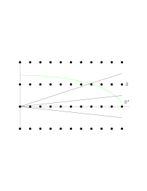
Figure 5: Two possible regions $S$ and $S^{\prime}$ containing supersymmetric vacua in a $K=2$ flux space. $S$ contains many fewer quantized flux points at small $L$ than its volume, while $S^{\prime}$ contains many more.

It is clear that $S$ is a cone; in other words $\lambda S\cong S$. Furthermore, for a small region $R$, the constraints $DW=0$ will not vary much, so one can think of $S$ as roughly a cone over the product of a $K/2-1$-dimensional sphere (at fixed radius in $\mathbb{R}^{K/2}$) with a $K/2$-dimensional ball. Over a small region, the constraint $N\eta N/2\leq L$ is not very different from a positive definite quadratic constraint, so $S_{L}$ is roughly the $r\leq\sqrt{L}$ part of this cone. For example, for $K=2$, one can have regions $S_{L}$ as pictured in figure 5.

Having characterized $S_{L}$, our goal is to count how many lattice points it contains. The most basic estimate is of course that, if we make $L$ sufficiently large, this number of lattice points will be well approximated by the volume of $S_{L}$. Furthermore, it is intuitively clear (see [21], 2.iv for more precise statements) that the leading correction to this is proportional to the surface area of the boundary of $S_{L}$, so for large $L$

$$N(L)=L^{K/2}V(S_{1})+L^{K/2-1/2}A(S_{1})+{\cal O}(L^{K/2-1/2-\epsilon})$$ (231)

where $V(S_{1})$ and $A(S_{1})$ are the volume and surface area at $L=1$.

How big need $L$ be to reach this scaling regime? In addition to the condition $L^{K/2}V(S_{1})>>1$ for the region to contain many lattice points, one clearly needs

$$\sqrt{L}>>{A(S_{1})\over V(S_{1})}$$ (232)

as well.

To illustrate what happens for smaller values of $L$, consider the case of $K=2$, and the two cones $S$ and $S^{\prime}$ illustrated in figure 5. Cone $S$, misaligned with the lattice, does not contain any lattice points near the origin. On the other hand, cone $S^{\prime}$, aligned with the lattice, contains roughly $r=\sqrt{L}$ (positive) lattice points within a small distance $r$ from the origin, far more than its volume $V\sim r^{2}\theta/2$ (where $\theta$ is the opening angle).

This phenomenon persists all the way out to $r\theta\sim 1$, at which point the two dimensional nature of the cones starts to be visible, and the estimate Eq. (231) becomes valid. This leads to the condition $r>1/\theta$. Since $V(S_{1})=\theta/2$ while $A(S_{1})\sim 2$, this is the same as Eq. (232).

Now the quantity $V(S_{1})$ is just the integrated vacuum density over the region $R$, and the quantity $A(S_{1})$ can be computed as an integral over moduli space using the same techniques. In the approximation that the vacuum density is just the volume form on moduli space, the surface area of the boundary will just be the surface area of the boundary in moduli space. Taking the region $R$ to be a sphere in moduli space of radius $r$, we find

$${A(S_{1})\over V(S_{1})}\sim{\sqrt{K}\over r}$$

so the condition Eq. (232) becomes

$$L>{K\over r^{2}}.$$ (233)

Thus, if we consider a large enough region, or the entire moduli space in order to find the total number of vacua, the condition for the asymptotic vacuum counting formulas we have discussed in this work to hold is $L>cK$ with some order one coefficient. But if we subdivide the region into subregions which do not satisfy Eq. (233), we will find that the number of vacua in each subregion will show oscillations around this central scaling. In fact, most regions will contain a smaller number of vacua (like $S$ above), while a few should have anomalously large numbers (like $S^{\prime}$ above), averaging out to Eq. (231).

5.1 Flux vacua on rigid Calabi-Yau

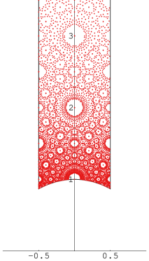
Figure 6: Values of $\tau$ for rigid CY flux vacua with $L_{max}=150$.

As an illustration of this, consider the following toy problem with $K=4$, studied in [1]. The configuration space is simply the fundamental region of the upper half plane, parameterized by $\tau$. The flux superpotentials are taken to be

$$W=A\tau+B$$

with $A=a_{1}+ia_{2}$ and $B=b_{1}+ib_{2}$ each taking values in $\mathbb{Z}+i\mathbb{Z}$. This would be obtained if we considered flux vacua on a rigid Calabi-Yau, with no complex structure moduli, $b_{3}=2$, and the periods $\Pi_{1}=1$ and $\Pi_{2}=i$. The tadpole condition $N\eta N/2\leq L$ becomes

$${\rm Im}A^{*}B\leq L$$ (234)

One then has

$$DW=0\leftrightarrow\bar{\tau}=-{B\over A}.$$ (235)

Thus, it is very easy to find all the vacua and the value of $\tau$ at which they are stabilized in this problem. We first enumerate all choices of $A$ and $B$ satisfying the bound Eq. (234), taking one representative of each orbit of the $SL(2,\mathbb{Z})$ duality group. As discussed in [1], this can be done by taking $a_{2}=0$, $0\leq b_{1}<a_{1}$ and $a_{1}b_{2}\leq L$. Then, for each choice of flux, we take the value of $\tau$ from Eq. (235) and map it into the fundamental region by an $SL(2,\mathbb{Z})$ transformation. The resulting plot for $L=150$ is shown in figure 6.

A striking feature of the figure is the presence of holes around points such as $\tau=ni$ with $n\in\mathbb{Z}$. At the center of such holes, there is moreover a big degeneracy of vacua. For example there are 240 vacua at $\tau=2i$. This clearly illustrates the phenomena discussed above. Starting with a tiny disk $D$ around $\tau=2i$, the corresponding cone in flux space is very narrow, but aligned with the lattice so it captures 240 points. For a somewhat displaced disk, the cone is not aligned with the lattice and captures no points. Increasing the radius of the disk makes the cone wider, and at a certain radius new lattice points enter.

Despite the intricate structure of the finite $L$ result, it is true that a disc of sufficiently large area $A$ will contain approximately $2\pi AL^{2}$ vacua. This is illustrated for $L=150$ in figure 7, where estimated and real numbers of vacua are compared in discs around $\tau=2i$ of stepwise increasing radius. Note that the first additional vacua enter the circle at a coordinate radius $R\sim 0.12$, and that just beyond that radius, at $R\sim 0.15$, the approximation becomes good. The corresponding radius in the proper metric is $r\sim 0.04$. Since the holes around the integers clearly correspond to the worst case scenario for the estimate, we can thus conclude empirically that for $L=150$, our estimate will be good when $r>0.04$. Moreover, by comparing the results for different values of $L$, we found that the radii of the holes scale precisely as $1/\sqrt{L}$. Thus, our empirical result for the reliability of the approximation is

$$r>{0.5\over\sqrt{L}},$$

which is compatible with Eq. (233).

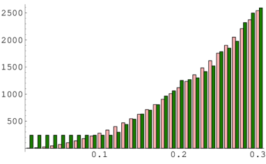
Figure 7: Number of vacua in a circle of coordinate radius $R$ around $\tau=2i$, with $R$ increasing in steps $dR=0.01$. Pink bars give the estimated value, green bars the actual value.

6 Conclusions

We gave general results for the distribution of supersymmetric and nonsupersymmetric flux vacua in type IIb string theory, and studied examples with one complex structure modulus in detail. Let us conclude with a brief summary of the results, some comparisons to what one might expect intuitively, and questions for further work.

A simplified picture of the results is that one can define an “average density of vacua” in the moduli space, which can be integrated over a region of interest and then multiplied by a “total number of allowed choices of flux,” to estimate the total number of vacua which stabilize moduli in that region. This estimate becomes exact in the limit of large flux, and should be good for flux satisfying the bounds discussed in section 5, say Eq. (233) for supersymmetric vacua.

The zeroth approximation for the average density of vacua is the volume form on moduli space constructed from the metric which would appear in the effective supergravity kinetic term; explicitly if this is

$$S_{moduli}=\int d^{4}xG_{ij}(z)\partial z^{i}\partial z^{j},$$

then we find

$$d\mu(z)\sim{\rm vol}={(2\pi L)^{K/2}\over(K/2)!}{1\over(\pi M_{p}^{2})^{n}}\sqrt{\det G(z)}d^{2n}z$$

in F theory and IIb flux compactification, with $K\sim B_{4}$ fluxes and tadpole bound $L$.

Of course, the actual results we obtained were of course more complicated, depending not just on the metric but on curvatures and its derivatives. However it is still useful to think of this “zeroth approximation” as the basic estimate, because in most of moduli space the curvatures are proportional to the metric up to $O(1)$ coefficients. In any case, this is the simplest distribution one can suggest which uses no data other than the effective theory itself, and is thus the “null hypothesis” in this class of problem.

In comparing our actual results to this, perhaps the most striking difference is the growth of vacuum density in regions of large curvature, for example near conifold points. The simple physical explanation in this case is that we know that the structure of the potential, or equivalently the dual gauge theory description of the physics, can produce a hierarchically small scale $\Lambda$. Since the average spacing between vacua is expected to be $\Lambda$, we can fit more vacua into such a region.

To make this quantitative, we need to understand the physics (or math) which makes the number of vacua finite. Here it is the tadpole condition, schematically $AB=L$ where $A$, $B$ are two conjugate types of flux, in dual terms controlling (say) the rank of the gauge group and the gauge coupling. A constraint $AB=L$ translates a distribution $dAdB$ into a scale invariant distribution $L~{}dA/A$.

In the large complex structure limit, the superpotential goes schematically as $A+B\tau^{k}$ for some power $k=1,2,3$. This leads to vacua at $\tau^{k}\sim A/B$, and the distribution $dA/A$ translates into $d^{2}\tau/{\rm Im}\tau^{2}$, taking into account supersymmetry which brings in the complexified modulus. Such a measure is naively scale invariant, and would lead to a diverging number of vacua. But, it is important that the integration region for ${\rm Re}\tau$ is $[0,1)$, so in fact the distribution falls off for large ${\rm Im}\tau$ and is integrable; the total number of vacua with $|\tau|>T$ goes as $1/T$. One can also understand this as a consequence of duality acting on the other fluxes, which leaves finitely many inequivalent choices (as in the toy example worked out in [1]).

Near a conifold, while the flux distribution is again roughly $L~{}dA/A$, the dual gauge theory-type superpotential $W=Az+Bz\log z$ leads to vacua at $\log z\sim A/B$ which have a $|d\log\log z|^{2}\sim d^{2}z/|z\log z|^{2}$ distribution. In fact, the distribution is rather similar to the previous one, with the identification $\tau=-\log z$. Whether this has deep significance is not clear to us; the large complex structure limit and conifold limit are not dual and in other ways are not similar. But it means that the number of vacua $N$ with a small scale $z<e^{-T}$, has a similar slow falloff, $N\sim 1/T$.

In some sense, many vacua are “Kähler stabilized” – if the Kähler potential were different, they would not exist. An illustration can be found in figure 4. As usual, this is less true for small $e^{\cal K}|W|^{2}$.

In section 5, we discussed the nature of the finite $L$ distribution of vacua. Because of flux quantization, this is far more complicated than the smooth distributions which we have been computing. On the other hand, one can say a lot about it using the smooth distributions and the methods we discussed. The basic idea is to think of the smooth distribution as computing a the volume of a region in flux space which supports vacua. Physical flux vacua satisfying flux quantization are lattice points in this region. While the volume of the region controls the large $L$ asymptotics, its other characteristics and in particular its surface area control the corrections to these asymptotics.

In particular, the smooth distribution will always approximate the finite $L$ distribution for sufficiently large $L$. However, the mimimal $L$ for this to be true depends on the size of the region in moduli space in which one is counting vacua, and can be estimated as $L\sim K/r^{2}$ for a ball of radius $r$. Thus, the number of vacua in a small region can deviate from the large $L$ distribution and even the $L^{K/2}$ asymptotic for the total number of vacua, until $L$ becomes quite large.

Another way to say this is that at finite $L$, to get a smooth density, one must average the number of vacua over regions in moduli space of size $r\sim\sqrt{K/L}$. The actual number of vacua in smaller regions will show oscillations, with most regions having many fewer vacua, and a few having many more vacua to make up for this. We discussed the simplest example in section 5, and a one complex modulus example is discussed in [24].

It is not inconceivable that these considerations could significantly decrease the total number of vacua in interesting examples with many cycles, if the geometric factors such as total volumes of Calabi-Yau moduli spaces were sufficiently small. Work on computing these volumes is in progress.

Let us move on to consider the results for specific types of vacua. First, we give the “null hypotheses” or simplest pictures which one might expect. First, F-type nonsupersymmetric vacua should be comparable in number to the supersymmetric vacua (given our definitions, this is obvious for the D-type), up to factors like $2^{n}$ where $n$ is the number of moduli. A heuristic argument for this is that the potential $V(z)$ is quadratic in $W(z)$, so if $W$ had been a polynomial of degree $d$, leading to $(d-1)^{n}$ vacua, then $V$ would be a polynomial of degree $2d$, suggesting $(2d-1)^{n}$ vacua. On reflection, the main problem with this argument is that the equations $V^{\prime}=0$ are real equations which typically have fewer than $(2d-1)^{n}$ solutions. Work on zeroes of randomly distributed polynomials with natural geometric distributions [19] suggests that in some cases, most zeroes are real, while in others there are many fewer real zeroes, so this is inconclusive. Finally, the metastability condition might be expected to be weak, in the sense that if the masses of bosons are distributed symmetrically about zero, the the fraction of tachyon free vacua would be $2^{-2n}$.

In general, these expectations do hold, and the number of non-supersymmetric vacua is comparable to the supersymmetric vacua. However, the number of metastable nonsupersymmetric vacua falls off drastically near conifold points, or more generally if the curvature on moduli space becomes large. This is rather surprising as naively the curvature contribution to the mass matrix Eq. (8) goes the other way; the conifold point has positive curvature which raises the masses. The explanation for the D type vacua is not complicated; it has to do with the special form of the mass matrix which leads to a “mixing” with the dilaton-axion which forces a mode tachyonic, as explained in 3.1. Some experimenting with multimodulus models suggests that this phenomenon is specific to one modulus and the detailed form of this potential, again in the D breaking case. We observed the same phenomenon for the F breaking; it may have a similar explanation.

We found in section 3.3 that the distribution of values of $e^{\cal K}|W|^{2}$ or “AdS cosmological constants” is typically uniform near zero, so that the fraction of vacua with $|\Lambda|<\Lambda_{*}$ behaves as $\Lambda_{*}/LT_{3}$. A simple argument for this was mentioned in [16]: for a given value of moduli, the magnitude of $W$ is a single direction in “flux space,” so the condition that it be small can be accomplished by one tuning of fluxes.

However, the fact that this tuning can be made independent of the choice of moduli is non-trivial. In problems such as the attractor mechanism with only one type of flux or charge for each cycle, it is not true. The heterotic string also has one type of flux per cycle and is formally very similar; one cannot get small AdS cosmological constant just from fluxes in this case. Of course, there are many more variables having to do with the gauge fields, which might make small cosmological constant possible in this problem.

The simple argument also misses a good deal of structure in the distribution; a good example is the behavior near the conifold point displayed in figure 4.

The heuristic argument that “nonsupersymmetric vacua are as common as supersymmetric” actually has a precise realization here, in the existence of vacua with $W=D^{2}W=0$. Since $W=0$ these are probably of limited physical interest, in particular it is hard to see how to stabilize their volume moduli. Other nonsupersymmetric vacua exist and are also roughly comparable in number. Strangely enough, the conditions of metastability and positive effective cosmological constant were incompatible, at least in the conifold and large structure limits. If this were generally true, and true in multi-modulus models, it would appear quite important.

Of course, all this was only a first cut at an actual counting of vacua. At this point it seems quite possible that many of the nonsupersymmetric vacua which are stable under variations of the moduli, have more subtle instabilities or inconsistencies. This would obviously be important to understand.

The scenario in which the numbers we are computing would be most meaningful would be one in which such effects drastically reduced the number of vacua, but in a way which was more or less uncorrelated to the distributions we studied. If we grant this, certain physical expectations would result. First, one finds that a high scale of supersymmetry breaking is favored (of course, this could be the scale in a hidden sector). This is already true in the D breaking vacua, for which at best the scale $M_{susy}^{4}$ is uniformly distributed, and in some cases (e.g. near conifold points) even disfavors small values. While we did not find F breaking vacua with positive cosmological constant, this may be an artifact of the one modulus case (or of the special limits we considered). But a high susy breaking scale would be even more favored for F breaking vacua in models with many moduli, as one expects the many supersymmetry breaking parameters $F_{i}=D_{i}W$ to be roughly independent and uniformly distributed.

The expectation that a high scale of supersymmetry breaking would lead to problems in tuning away the cosmological constant, favoring a low scale of breaking, is probably not true for these vacua. The point is that the contribution to the energy which does this tuning, the $-3e^{\cal K}|W|^{2}$ term or “AdS cosmological constant,” gets contributions from many sectors of the theory, including sectors with unbroken supersymmetry, and has no a priori correlation to the supersymmetry breaking scale. Given a particular supersymmetry breaking scale, this contribution is then set by the requirement that $\Lambda\sim 0$, but since in general vacua exist with a uniform distribution of this parameter, this condition in itself does not favor any particular scale.

Thus, these distributions seem to favor “moduli dominated gravity mediated supersymmetry breaking,” in the terminology of [9]. One has a general prediction of a large gravitino mass, and risks the common problems of supergravity mediated breaking, such as non-universal soft breaking terms. Perhaps this is less of a problem in the D breaking models.

Finally, the moduli space measure (the metric on the space of metrics) heavily disfavors large complex structure and large volume in the many modulus models, as we will discuss in more depth in [11].

Acknowledgements

We thank B. Acharya, B. Florea, S. Kachru, R. Kallosh, G. Moore, B. Shiffman, S. Shenker, E. Silverstein, S. Thomas, P.M.H. Wilson, E. Witten, S.-T. Yau and S. Zelditch for discussions and correspondence. We particularly thank S. Kachru for communications regarding the work [24] in progress, which stimulated us to revise section 5.

This research was supported in part by DOE grant DE-FG02-96ER40959. M.R.D. is supported by the Gordon Moore Distinguished Scholar program at Caltech.

References

- [1] S. Ashok and M. R. Douglas, Counting Flux Vacua, JHEP 0401 (2004) 060 [arXiv:hep-th/0307049]
- [2] P. S. Aspinwall and M. R. Douglas, D-brane stability and monodromy, JHEP 0205, 031 (2002) [arXiv:hep-th/0110071].
- [3] T. Banks, M. Dine and E. Gorbatov, Is There A String Theory Landscape, [arXiv:hep-th/0309170].
- [4] K. Behrndt, S. Gukov and M. Shmakova, Domain walls, black holes, and supersymmetric quantum mechanics, Nucl. Phys. B 601, 49 (2001) [arXiv:hep-th/0101119].
- [5] P. Binetruy, G. Dvali, R. Kallosh and A. Van Proeyen, Fayet-Iliopoulos terms in supergravity and cosmology, [arXiv:hep-th/0402046].
- [6] R. Bousso and J. Polchinski, “Quantization of four-form fluxes and dynamical neutralization of the cosmological constant,” JHEP 0006, 006 (2000) [arXiv:hep-th/0004134].
- [7] I. Brunner and K. Hori, “Orientifolds and Mirror Symmetry,” [arXiv:hep-th/0303135].
- [8] P. Candelas, X. C. De La Ossa, P. S. Green and L. Parkes, A Pair Of Calabi-Yau Manifolds As An Exactly Soluble Superconformal Theory, Nucl. Phys. B 359, 21 (1991).
- [9] D. J. H. Chung, L. L. Everett, G. L. Kane, S. F. King, J. Lykken and L. T. Wang, The soft supersymmetry-breaking Lagrangian: Theory and applications, to appear in Physics Reports, [arXiv:hep-ph/0312378].
- [10] F. Denef, B. R. Greene and M. Raugas, “Split Attractor Flows and the Spectrum of BPS D-branes on the Quintic,” JHEP 0105, 012 (2001) [arXiv:hep-th/0101135].
- [11] F. Denef and M. R. Douglas, to appear.
- [12] F. Denef, M. R. Douglas and B. Florea, to appear.
- [13] O. DeWolfe, S. Kachru and H. Verlinde, “The giant inflaton,” arXiv:hep-th/0403123.
- [14] M. R. Douglas, The statistics of string/M theory vacua. JHEP 0305 (2003) 046 [arXiv:hep-th/0303194]
- [15] M. R. Douglas, B. Shiffman and S. Zelditch, Critical points and supersymmetric vacua, submitted to Comm. Math. Phys, [arXiv:math.CV/0402326].
- [16] M. R. Douglas, Statistics of String Vacua, to appear in the proceedings of the Workshop on String Phenomenology at Durham, UK, August 2003, [arXiv:hep-ph/0401004].
- [17] M. R. Douglas, Mastering , in the on-line proceedings of Strings 2002, Cambridge UK.
- [18] M. R. Douglas, D-Branes and N=1 Supersymmetry, in the proceedings of Strings 2001, Mumbai, India. [arXiv:hep-th/0105014].
- [19] A. Edelman and E. Kostlan, How many zeros of a random polynomial are real?, Bull. Amer. Math. Soc. (N.S.) 32 (1995) 1-37, [arXiv:math.CA/9501224].
- [20] A. R. Frey and J. Polchinski, N = 3 warped compactifications, Phys. Rev. D 65, 126009 (2002) [arXiv:hep-th/0201029].
- [21] Geometry of Numbers, P. M. Gruber and C. G. Lekkerkerker, North-Holland, 1987.
- [22] S. B. Giddings, S. Kachru and J. Polchinski, Hierarchies from fluxes in string compactifications, Phys. Rev. D 66, 106006 (2002) [arXiv:hep-th/0105097].
- [23] A. Giryavets, S. Kachru, P. K. Tripathy and S. P. Trivedi, Flux compactifications on Calabi-Yau threefolds, arXiv:hep-th/0312104.
- [24] A. Giryavets, S. Kachru, P. K. Tripathy and S. P. Trivedi, to appear.
- [25] T. W. Grimm and J. Louis, The effective action of N = 1 Calabi-Yau orientifolds, arXiv:hep-th/0403067.
- [26] S. Gukov, C. Vafa and E. Witten, CFT’s from Calabi-Yau four-folds, Nucl. Phys. B 584, 69 (2000) [Erratum-ibid. B 608, 477 (2001)] [arXiv:hep-th/9906070].
- [27] S. Kachru, J. Pearson and H. Verlinde, “Brane/flux annihilation and the string dual of a non-supersymmetric field theory,” JHEP 0206, 021 (2002) [arXiv:hep-th/0112197].
- [28] S. Kachru, M. B. Schulz and S. Trivedi, Moduli stabilization from fluxes in a simple IIB orientifold, JHEP 0310, 007 (2003) [arXiv:hep-th/0201028].
- [29] S. Kachru, R. Kallosh, A. Linde and S. P. Trivedi, De Sitter vacua in string theory, Phys. Rev. D 68, 046005 (2003); [arXiv:hep-th/0301240].
- [30] G. W. Moore, “Arithmetic and attractors,” arXiv:hep-th/9807087.
- [31] A. Strominger, Superstrings with Torsion, Nucl. Phys. B274 (1986) 253.
- [32] E. Witten, On flux quantization in M-theory and the effective action, J. Geom. Phys. 22, 1 (1997) [arXiv:hep-th/9609122].