Quantum weights of dyons and of instantons with non-trivial holonomy

Abstract

We calculate exactly functional determinants for quantum oscillations about periodic instantons with non-trivial value of the Polyakov line at spatial infinity. Hence, we find the weight or the probability with which calorons with non-trivial holonomy occur in the Yang–Mills partition function. The weight depends on the value of the holonomy, the temperature, $\Lambda_{\rm QCD}$, and the separation between the BPS monopoles (or dyons) which constitute the periodic instanton. At large separation between constituent dyons, the quantum measure factorizes into a product of individual dyon measures, times a definite interaction energy. We present an argument that at temperatures below a critical one related to $\Lambda_{\rm QCD}$, trivial holonomy is unstable, and that calorons “ionize” into separate dyons.

I Motivation and the main result

There are two known generalizations of the standard self-dual instantons to non-zero temperatures. One is the periodic instanton of Harrington and Shepard HS studied in detail by Gross, Pisarski and Yaffe  GPY . These periodic instantons, also called calorons, are said to have trivial holonomy at spatial infinity. It means that the Polyakov line

$$L=\left.{\rm P}\,\exp\left(\int_{0}^{1/T}\!dt\,A_{4}\right)\right|_{|\vec{x}|\to\infty}$$ (1)

assumes values belonging to the group center $Z(N)$ for the $SU(N)$ gauge group . The vacuum made of those instantons has been investigated, using the variational principle, in ref. DMir .

The other generalization has been constructed a few years ago by Kraan and van Baal KvB and Lee and Lu LL ; it has been named caloron with non-trivial holonomy as the Polyakov line for this configuration does not belong to the group center. We shall call it for short the KvBLL caloron. It is also a periodic self-dual solution of the Yang–Mills equations of motion with an integer topological charge. In the limiting case when the KvBLL caloron is characterized by trivial holonomy, it is reduced to the Harrington–Shepard caloron. The fascinating feature of the KvBLL construction is that a caloron with a unit topological charge can be viewed as “made of” $N$ Bogomolnyi–Prasad–Sommerfeld (BPS) monopoles or dyons Bog ; PS .

Dyons are self-dual solutions of the Yang–Mills equations of motion with static (i.e. time-independent) action density, which have both the magnetic and electric field at infinity decaying as $1/r^{2}$. Therefore these objects carry both electric and magnetic charges (prompting their name). In the $3\!+\!1$-dimensional $SU(2)$ gauge theory there are in fact two types of self-dual dyons LY : $M$ and $L$ with (electric, magnetic) charges $(+,+)$ and $(-,-)$, and two types of anti-self-dual dyons $\overline{M}$ and $\overline{L}$ with charges $(+,-)$ and $(-,+)$, respectively. Their explicit fields can be found e.g. in ref. DPSUSY . In the $SU(N)$ theory there are $2N$ different dyons LY ; DHKM : $M_{1},M_{2},...M_{N-1}$ ones with charges counted with respect to $N-1$ Cartan generators and one $L$ dyon with charges compensating those of $M_{1}...M_{N-1}$ to zero, and their anti-self-dual counterparts.

Speaking of dyons one implies that the Euclidean space-time is compactified in the ‘time’ direction whose inverse circumference is temperature $T$, with the usual periodic boundary conditions for boson fields. However, the temperature may go to zero, in which case the $4d$ Euclidean invariance is restored.

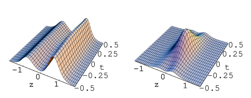
Figure 1: The action density of the KvBLL caloron as function of $z,t$ at fixed $x=y=0$, with the asymptotic value of $A_{4}$ at spatial infinity ${\rm v}=0.9\pi T,\;\overline{{\rm v}}=1.1\pi T$. It is periodic in $t$ direction. At large dyon separation the density becomes static (left, $r_{12}=1.5/T$). As the separation decreases the action density becomes more like a $4d$ lump (right, $r_{12}=0.6/T$). In both plots the L,M dyons are centered at $z_{\rm L}=-{\rm v}\,r_{12}/2\pi T,\;z_{\rm M}=\overline{{\rm v}}\,r_{12}/2\pi T,\;x_{\rm L,M}=y_{\rm L,M}=0$. The axes are in units of temperature T.

Dyons’ essence is that the $A_{4}$ component of the dyon field tends to a constant value at spatial infinity. This constant $A_{4}$ can be eliminated by a time-dependent gauge transformation. However then the fields violate the periodic boundary conditions, unless $A_{4}$ has quantized values corresponding to trivial holonomy, i.e. unless the Polyakov line belongs to the group center. Therefore, in a general case one implies that dyons have a non-zero value of $A_{4}$ at spatial infinity and a non-trivial holonomy.

The KvBLL caloron of the $SU(2)$ gauge group (to which we restrict ourselves in this paper) with a unit topological charge is “made of” one $L$ and one $M$ dyon, with total zero electric and magnetic charges. Although the action density of isolated $L$ and $M$ dyons does not depend on time, their combination in the KvBLL solution is generally non-static: the $L,M$ “constituents” show up not as $3d$ but rather as $4d$ lumps, see Fig. 1. When the temperature goes to zero while the separation between dyons remain fixed, these lumps merge, and the KvBLL caloron is reduced to the usual Belavin–Polyakov–Schwarz–Tyutin instanton BPST (as is the standard Harrington–Shepard caloron), plus corrections of the order of $T$. However, the holonomy remains fixed and non-trivial at spatial infinity.

There is a strong argument against the presence of either dyons or KvBLL calorons in the Yang–Mills partition function at nonzero temperatures GPY . The point is, the 1-loop effective action obtained from integrating out fast varying fields where one keeps all powers of $A_{4}$ but expands in (covariant) derivatives of $A_{4}$ has the form DO

$$S^{\rm 1-loop} = \int\!d^{4}x\,\left[P(A_{4})+E^{2}f_{E}(A_{4})+B^{2}f_{B}(A_{4})+{\rm higher\;derivative\;terms}\right],$$

$$P(A_{4}) = \left.\frac{1}{3T(2\pi)^{2}}{\rm v}^{2}(2\pi T-{\rm v})^{2}\right|_{{\rm mod}\;2\pi T},\qquad{\rm v}=\sqrt{A_{4}^{a}A_{4}^{a}}\qquad[{\rm for\;the}\;SU(2)\;{\rm group}]$$ (2)

where the perturbative potential energy term $P(A_{4})$ has been known for a long time GPY ; NW , see Fig. 2. As follows from eq.(1) the trace of the Polyakov line is related to ${\rm v}$ as

$$\frac{1}{2}\,{\rm Tr}\,L=\cos\frac{{\rm v}}{2T}.$$ (3)

The zeros of the potential energy correspond to $\frac{1}{2}{\rm Tr}\,L=\pm 1$, i.e. to the trivial holonomy. If a dyon has ${\rm v}\neq 2\pi Tn$ at spatial infinity the potential energy is positive-definite and proportional to the $3d$ volume. Therefore, dyons and KvBLL calorons with non-trivial holonomy seem to be strictly forbidden: quantum fluctuations about them have an unacceptably large action.

Meanwhile, precisely these objects determine the physics of the supersymmetric YM theory where in addition to gluons there are gluinos, i.e. Majorana (or Weyl) fermions in the adjoint representation. Because of supersymmetry, the boson and fermion determinants about $L,M$ dyons cancel exactly, so that the perturbative potential energy (2) is identically zero for all temperatures, actually in all loops. Therefore, in the supersymmetric theory dyons are openly allowed. [To be more precise, the cancellation occurs when periodic conditions for gluinos are imposed, so it is the compactification in one (time) direction that is implied, rather than physical temperature which requires antiperiodic fermions.] Moreover, it turns out DHKM that dyons generate a non-perturbative potential having a minimum at ${\rm v}=\pi T$, i.e. where the perturbative potential would have the maximum. This value of $A_{4}$ corresponds to the holonomy ${\rm Tr}\,L=0$ at spatial infinity, which is the “most non-trivial”; as a matter of fact $<\!{\rm Tr}\,L\!>=0$ is one of the confinement’s requirements. In the supersymmetric YM theory configurations having ${\rm Tr}\,L=0$ at infinity are not only allowed but dynamically preferred as compared to those with $\frac{1}{2}{\rm Tr}\,L=\pm 1$. In non-supersymmetric theory it looks as if it is the opposite.

Nevertheless, it has been argued in ref. Dobzor that the perturbative potential energy (2) which forbids individual dyons in the pure YM theory might be overruled by non-perturbative contributions of an ensemble of dyons. For fixed dyon density, their number is proportional to the $3d$ volume and hence the non-perturbative dyon-induced potential as function of the holonomy (or of $A_{4}$ at spatial infinity) is also proportional to the volume. It may be that at temperatures below some critical one the non-perturbative potential wins over the perturbative one so that the system prefers $<\!{\rm Tr}\,L\!>=0$. This scenario could then serve as a microscopic mechanism of the confinement-deconfinement phase transition Dobzor . It should be noted that the KvBLL calorons and dyons seem to be observed in lattice simulations below the phase transition temperature Brower ; IMMPSV ; Gatt .

To study this possible scenario quantitatively, one first needs to find out the quantum weight of dyons or the probability with which they appear in the Yang–Mills partition function. Unfortunately, the single-dyon measure is not well defined: it is too badly divergent in the infrared region owing to the weak (Coulomb-like) decrease of the fields. What makes sense and is finite, is the quantum determinant for small oscillations about the KvBLL caloron which possesses zero net electric and magnetic charges. To find this determinant is the primary objective of this study. The KvBLL measure depends on the asymptotic value of $A_{4}$ (or on the holonomy through eq.(3)), on the temperature $T$, on $\Lambda$, the scale parameter obtained through the renormalization of the charge, and on the dyon separation $r_{12}$. At large separations between constituent $L,M$ dyons of the caloron, one gets their weights and their interaction.

The problem of computing the effect of quantum fluctuations about a caloron with non-trivial holonomy is of the same kind as that for ordinary instantons (solved by ’t Hooft tHooft ) and for the standard Harrington–Shepard caloron (solved by Gross, Pisarski and Yaffe GPY ) being, however, technically much more difficult. The zero-temperature instanton is $O(4)$ symmetric, and the Harrington–Shepard caloron is $O(3)$ symmetric, which helps. The KvBLL caloron has no such symmetry as obvious from Fig. 1. Nevertheless, we have managed to find the small-oscillation determinant exactly. It becomes possible because we are able to construct the exact propagator of spin-0, isospin-1 field in the KvBLL background, which by itself is some achievement.

As it is well known tHooft ; GPY , the calculation of the quantum weight of a Euclidean pseudoparticle consists of three steps: i) calculation of the metric of the moduli space or, in other words, computing the Jacobian composed of zero modes, needed to write down the pseudoparticle measure in terms of its collective coordinates, ii) calculation of the functional determinant for non-zero modes of small fluctuations about a pseudoparticle, iii) calculation of the ghost determinant resulting from background gauge fixing in the previous step. Problem i) has been actually solved already by Kraan and van Baal KvB . Problem ii) is reduced to iii) in the self-dual background field BC since for such fields ${\rm Det}(W_{\mu\nu})={\rm Det}(-D^{2})^{4}$, where $W_{\mu\nu}$ is the quadratic form for spin-1, isospin-1 quantum fluctuations and $D^{2}$ is the covariant Laplace operator for spin-0, isospin-1 ghost fields. Symbolically, one can write

$${\rm KvBLL\;measure}=\int\!d({\rm collective\;coordinates})\cdot{\rm Jacobian}\cdot{\rm Det}^{-\frac{1}{2}}(W_{\mu\nu})\cdot{\rm Det}(-D^{2})$$ (4)

where the product of the last two factors is simply ${\rm Det}^{-1}(-D^{2})$ in the self-dual background. As usually, the functional determinants are normalized to free ones (with zero background fields) and UV regularized (we use the standard Pauli–Villars method). Thus, to find the quantum weight of the KvBLL caloron only the ghost determinant has to be computed.

To that end, we follow Zarembo Zar and find the derivative of this determinant with respect to the holonomy or, more precisely, to ${\rm v}\equiv\left.\sqrt{A_{4}^{a}A_{4}^{a}}\right|_{|\vec{x}|\to\infty}$. The derivative is expressed through the Green function of the ghost field in the caloron background. If a self-dual field is written in terms of the Atiah–Drinfeld–Hitchin–Manin construction, and in the KvBLL case it basically is KvB ; LL , the Green function is generally known Adler -Nahm80 and we build it explicitly for the KvBLL case. Therefore, we are able to find the derivative $\partial{\rm Det}(-D^{2})/\partial{\rm v}$. Next, we reconstruct the full determinant by integrating over ${\rm v}$ using the determinant for the trivial holonomy GPY as a boundary condition. This determinant at ${\rm v}=0$ is still a non-trivial function of $r_{12}$ and the fact that we match it from the ${\rm v}\neq 0$ side is a serious check. Actually we need only one overall constant factor from ref. GPY in order to restore the full determinant at ${\rm v}\neq 0$, and we make a minor improvement of the Gross–Pisarski–Yaffe calculation as we have computed the needed constant analytically.

Although all the above steps can be performed explicitly, at some point the equations become extremely lengthy – typical expressions are several Mbytes long and so far we have not managed to simplify them such that they would fit into a paper. However, we are able to obtain compact analytical expressions in the physically interesting case of large separation between dyons, $r_{12}\gg 1/T$. We have also used the exact formulae to check numerically some of the intermediate formulae, in particular at ${\rm v}\to 0$.

If the separation is large in the temperature scale, $r_{12}\gg 1/T$, the final result for the quantum measure of the KvBLL caloron can be written down in terms of the $3d$ positions of the two constituent $L,M$ dyons $\vec{z}_{1,2}$, their separation $r_{12}=|\vec{z}_{1}-\vec{z}_{2}|$, the asymptotic of $A_{4}$ at spatial infinity denoted by ${\rm v}\in[0,2\pi T]$ and $\overline{{\rm v}}=2\pi T-{\rm v}\in[0,2\pi T]$, see eq.(80). We give here a simpler expression obtained in the limit when the separation between dyons is much larger than their core sizes:

$${\cal Z}_{\rm KvBLL} = \int d^{3}z_{1}\,d^{3}z_{2}\,T^{6}\,(2\pi)^{\frac{8}{3}}\,C\,\left(\frac{8\pi^{2}}{g^{2}}\right)^{4}\left(\frac{\Lambda e^{\gamma_{E}}}{4\pi T}\right)^{\frac{22}{3}}\left(\frac{{\rm v}}{2\pi T}\right)^{\frac{4{\rm v}}{3\pi T}}\left(\frac{\overline{{\rm v}}}{2\pi T}\right)^{\frac{4\overline{{\rm v}}}{3\pi T}}$$ (5)

$$\times \exp\left[-2\pi\,r_{12}\,P^{\prime\prime}({\rm v})\right]\;\exp\left[-V^{(3)}P({\rm v})\right],$$

where the overall factor $C$ is a combination of universal constants; numerically $C=1.031419972084$. $\Lambda$ is the scale parameter in the Pauli–Villars scheme; the factor $g^{-8}$ is not renormalized at the one-loop level.

Since the caloron field has a constant $A_{4}$ component at spatial infinity, it is suppressed by the same perturbative potential $P({\rm v})$ as given by eq.(2). Its second derivative with respect to ${\rm v}$ is $P^{\prime\prime}({\rm v})=\frac{1}{\pi^{2}T}\left[v\!-\!\pi T\left(1\!-\!\frac{1}{\sqrt{3}}\right)\right]\left[v\!-\!\pi T\left(1\!+\!\frac{1}{\sqrt{3}}\right)\right]$. If ${\rm v}$ is in the ranges between 0 and $\pi T\left(1\!-\!\frac{1}{\sqrt{3}}\right)$ or between $\pi T\left(1\!+\!\frac{1}{\sqrt{3}}\right)$ and $2\pi T$ (corresponding to the holonomy not too far from the trivial, $0.787597\!<\!\frac{1}{2}|{\rm Tr}L|\!<\!1$) the second derivative $P^{\prime\prime}({\rm v})$ is positive, and the $L$ and $M$ dyons experience a linear attractive potential. Integration over the separation $r_{12}$ of dyons inside a caloron converges. We perform this integration in section VII, estimate the free energy of the caloron gas and conclude that trivial holonomy (${\rm v}=0,2\pi T$) may be unstable, despite the perturbative potential energy $P({\rm v})$. In the complementary range $\pi T\left(1\!-\!\frac{1}{\sqrt{3}}\right)\!<\!{\rm v}\!<\!\pi T\left(1\!+\!\frac{1}{\sqrt{3}}\right)$ (or $\frac{1}{2}|{\rm Tr}L|\!<\!0.787597$), $P^{\prime\prime}({\rm v})$ is negative (see Fig. 2), and dyons experience a strong linear-rising repulsion. It means that for these values of ${\rm v}$, integration over the dyon separations diverges: calorons with holonomy far from trivial “ionize” into separate dyons.

II The KvBLL caloron solution

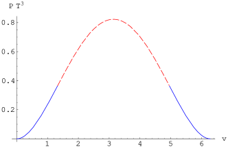
Figure 2: Potential energy as function of ${\rm v}/T$. Two minima correspond to $\frac{1}{2}{\rm Tr}L=\pm 1$, the maximum corresponds to ${\rm Tr}L=0$. The range of the holonomy where dyons experience repulsion is shown in dashing.

Although the construction of the self-dual solution with non-trivial holonomy has been fully performed independently by Kraan and van Baal KvB and Lee and Lu LL we have found it more convenient for our purposes to use the gauge convention and the formalism of Kraan and van Baal (KvB) whose notations we follow in this paper.

The key quantities characterizing the KvBLL solution for a general $SU(N)$ gauge group are the $N\!-\!1$ gauge-invariant eigenvalues of the Polyakov line (1) at spatial infinity. For the $SU(2)$ gauge group to which we restrict ourselves in this paper, it is just one quantity, e.g. ${\rm Tr}\,L$, eq.(3). In a gauge where $A_{4}$ is static and diagonal at spatial infinity, i.e. $\left.A_{4}\right|_{{\vec{x}}\to\infty}=i{\rm v}\frac{\tau_{3}}{2}$, it is this asymptotic value ${\rm v}$ which characterizes the caloron solution in the first place. We shall also use the complementary quantity $\overline{{\rm v}}\equiv 2\pi T-{\rm v}$. Their relation to parameters $\omega,\bar{\omega}$ introduced by KvB KvB is $\omega=\frac{{\rm v}}{4\pi T},\;\bar{\omega}=\frac{\overline{{\rm v}}}{4\pi T}=\frac{1}{2}-\omega$. Both ${\rm v}$ and $\overline{{\rm v}}$ vary from 0 to $2\pi T$. At ${\rm v}=0,2\pi T$ the holonomy is said to be ‘trivial’, and the KvBLL caloron reduces to that of Harrington and Shepard HS .

There are, of course, many ways to parametrize the caloron solution. Keeping in mind that we shall be mostly interested in the case of widely separated dyon constituents, we shall parametrize the solution in terms of the coordinates of the dyons’ ‘centers’ (we call constituent dyons L and M according to the classification in ref. DPSUSY ):

$$L\;{\rm dyon}:\quad \vec{z}_{1}=-\frac{2\omega{\overrightarrow{r_{12}}}}{T},$$

$$M\;{\rm dyon}:\quad \vec{z}_{2}=\frac{2\bar{\omega}{\overrightarrow{r_{12}}}}{T},$$

$${\rm dyon\;separation}: \vec{z}_{2}-\vec{z}_{1}={\overrightarrow{r_{12}}},\quad\quad|r_{12}|=\pi T\,\rho^{2},$$

where $\rho$ is the parameter used by KvB; it becomes the size of the instanton at ${\rm v}\to 0$. We introduce the distances from the ‘observation point’ $\vec{x}$ to the dyon centers,

$$\vec{r}=\vec{x}-\vec{z}_{1}=\vec{x}+2\omega\overrightarrow{r_{12}},\qquad r=|\vec{r}|,$$

$$\vec{s}=\vec{x}-\vec{z}_{2}=\vec{x}-2\bar{\omega}\overrightarrow{r_{12}},\qquad s=|\vec{s}|.$$ (6)

Henceforth we measure all dimensional quantities in units of temperature for brevity and restore $T$ explicitly only in the final results.

The KvBLL caloron field in the fundamental representation is KvB (we choose the separation between dyons to be in the third spatial direction, ${\overrightarrow{r_{12}}}=r_{12}\vec{e}_{3}$):

$$A_{\mu}=\delta_{\mu,4}\,i{\rm v}\frac{\tau_{3}}{2}+\frac{i}{2}\bar{\eta}^{3}_{\mu\nu}\tau_{3}\partial_{\nu}\ln\Phi+\frac{i}{2}\Phi\;{\rm Re}\left[(\bar{\eta}^{1}_{\mu\nu}-i\bar{\eta}^{2}_{\mu\nu})(\tau_{1}+i\tau_{2})(\partial_{\nu}+i{\rm v}\delta_{\nu,4})\tilde{\chi}\right]\,,$$ (7)

where $\tau_{i}$ are Pauli matrices, $\bar{\eta}^{a}_{\mu\nu}$ are ’t Hooft’s symbols tHooft with $\bar{\eta}^{a}_{ij}=\epsilon_{aij}$ and $\bar{\eta}^{a}_{4\nu}=-\bar{\eta}^{a}_{\nu 4}=i\delta_{a\nu}$. “Re” means $2{\rm Re}(W)\equiv W+W^{\dagger}$ and the functions used are

$$\hat{\psi}=-\cos(2\pi x_{4})+\overline{\mathrm{ch}}\,\mathrm{ch}\,+\frac{\vec{r}\vec{s}}{2rs}\overline{\mathrm{sh}}\,\mathrm{sh}\,,\qquad\psi=\hat{\psi}+\frac{r_{12}^{2}}{rs}\overline{\mathrm{sh}}\,\mathrm{sh}\,+\frac{r_{12}}{s}\mathrm{sh}\,\overline{\mathrm{ch}}\,+\frac{r_{12}}{r}\overline{\mathrm{sh}}\,\mathrm{ch}\,,$$

$$\tilde{\chi}=\frac{r_{12}}{\psi}\left(e^{-2\pi ix_{4}}\frac{\mathrm{sh}\,}{s}+\frac{\overline{\mathrm{sh}}\,}{r}\right),\qquad\Phi=\frac{\psi}{\hat{\psi}}\,.$$ (8)

We have introduced short-hand notations for hyperbolic functions:

$$\mathrm{sh}\,\equiv\sinh(s{\rm v}),\qquad\mathrm{ch}\,\equiv\cosh(s{\rm v}),\qquad\overline{\mathrm{sh}}\,\equiv\sinh(r\overline{{\rm v}}),\qquad\overline{\mathrm{ch}}\,\equiv\cosh(r\overline{{\rm v}})\,.$$ (9)

The first term in (7) corresponds to a constant $A_{4}$ component at spatial infinity ($A_{4}\approx i{\rm v}\frac{\tau_{3}}{2}$) and gives rise to the non-trivial holonomy. One can see that $A_{\mu}$ is periodic in time with period $1$ (since we have chosen the temperature to be equal to unity). A useful formula for the field strength squared is KvB

$${\rm Tr}\,F_{\mu\nu}F_{\mu\nu}=\partial^{2}\partial^{2}\log\psi.$$ (10)

In the situation when the separation between dyons $r_{12}$ is large compared to both their core sizes $\frac{1}{{\rm v}}$ (M) and $\frac{1}{\overline{{\rm v}}}$ (L), the caloron field can be approximated by the sum of individual BPS dyons, see Figs. 1,3 (left) and Fig. 4. We give below the field inside the cores and far away from both cores.

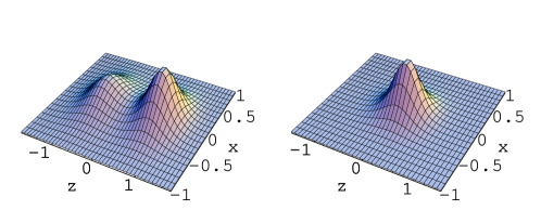
Figure 3: The action density of the KvBLL caloron as function of $z,x$ at fixed $t=y=0$. At large separations $r_{12}$ the caloron is a superposition of two BPS dyon solutions (left, $r_{12}=1.5/T$). At small separations they merge (right, $r_{12}=0.6/T$). The caloron parameters are the same as in Fig. 1.

II.1 Inside dyon cores

In the vicinity of the L dyon center $\vec{z}_{1}$ and far away from the M dyon ($s{\rm v}\gg 1$) the field becomes that of the L dyon. It is instructive to write it in spherical coordinates centered at $\vec{z}_{1}$. In the ‘stringy’ gauge DPSUSY in which the $A_{4}$ component is constant and diagonal at spatial infinity, the L dyon field is

$$A_{4}^{L} = \frac{i\tau_{3}}{2}\left(\frac{1}{r}+2\pi-\overline{{\rm v}}\coth(\overline{{\rm v}}r)\right),\;\;\;A^{L}_{r}=0,$$

$$A^{L}_{\theta} = i\overline{{\rm v}}\frac{-\sin(2\pi x_{4}-\phi)\;\tau_{1}+\cos(2\pi x_{4}-\phi)\tau_{2}}{2\sinh(\overline{{\rm v}}r)},$$

$$A^{L}_{\phi} = i\overline{{\rm v}}\frac{\cos(2\pi x_{4}-\phi)\;\tau_{1}+\sin(2\pi x_{4}-\phi)\tau_{2}}{2\sinh(\overline{{\rm v}}r)}-i\tau_{3}\frac{\tan(\theta/2)}{2r}\;.$$ (11)

Here $A_{\theta}$, for example, is the projection of $\vec{A}$ onto the direction $\vec{n}_{\theta}=(\cos\theta\cos\phi,\cos\theta\sin\phi,-\sin\theta)$. The $\phi$ component has a string singularity along the $z$ axis going in the positive direction. Notice that inside the core region ($\overline{{\rm v}}r\leq 1$) the field is time-dependent, although the action density is static. At large distances from the L dyon center, i.e. far outside the core one neglects exponentially small terms ${\cal O}\left(e^{-\overline{{\rm v}}r}\right)$ and the surviving components are

$$A^{L}_{4} \stackrel{{\scriptstyle r\to\infty}}{{\longrightarrow}} \left({\rm v}+\frac{1}{r}\right)\,\frac{i\tau^{3}}{2},$$

$$A^{L}_{\phi} \stackrel{{\scriptstyle r\to\infty}}{{\longrightarrow}} -\frac{{\rm tan}\frac{\theta}{2}}{r}\,\frac{i\tau^{3}}{2}$$

corresponding to the radial electric and magnetic field components

$$E^{L}_{r}=B^{L}_{r}\stackrel{{\scriptstyle r\to\infty}}{{\longrightarrow}}-\frac{1}{r^{2}}\,\frac{i\tau^{3}}{2}.$$ (12)

This Coulomb-type behavior of both the electric and magnetic fields prompts the name ‘dyon’.

Similarly, in the vicinity of the M dyon and far away from the L dyon ($r\overline{{\rm v}}\gg 1$) the field becomes that of the M dyon, which we write in spherical coordinates centered at $\vec{z}_{2}$:

$$A_{4}^{M}=\frac{i\tau_{3}}{2}\left({\rm v}\coth({\rm v}s)-\frac{1}{s}\right),\quad A_{\theta}^{M}={\rm v}\frac{\sin\!\phi\;\tau_{1}-\cos\!\phi\;\tau_{2}}{2i\sinh({\rm v}s)}\,,$$

$$A_{r}^{M}=0,\quad A_{\phi}^{M}={\rm v}\frac{\cos\!\phi\;\tau_{1}+\sin\!\phi\;\tau_{2}}{2i\sinh({\rm v}s)}+i\tau_{3}\frac{\tan(\theta/2)}{2s},$$ (13)

whose asymptotics is

$$A^{M}_{4} \stackrel{{\scriptstyle r\to\infty}}{{\longrightarrow}} \left({\rm v}-\frac{1}{s}\right)\,\frac{i\tau^{3}}{2},$$

$$A^{M}_{\phi} \stackrel{{\scriptstyle r\to\infty}}{{\longrightarrow}} \frac{{\rm tan}\frac{\theta}{2}}{s}\,\frac{i\tau^{3}}{2},$$

$$E^{M}_{r}=B^{M}_{r} \stackrel{{\scriptstyle r\to\infty}}{{\longrightarrow}} \frac{1}{s^{2}}\,\frac{i\tau^{3}}{2}.$$ (14)

We see that in both cases the L,M fields become Abelian at large distances, corresponding to (electric, magnetic) charges $(-,-)$ and $(+,+)$, respectively. The corrections to the fields (11,13) are hence of the order of $1/r_{12}$ arising from the presence of the other dyon.

II.2 Far away from dyon cores

Far away from both dyon cores ($r\overline{{\rm v}}\gg 1,\;s{\rm v}\gg 1$; note that it does not necessarily imply large separations – the dyons may even be overlapping) one can neglect both types of exponentially small terms, ${\cal O}\left(e^{-r\overline{{\rm v}}}\right)$ and ${\cal O}\left(e^{-s{\rm v}}\right)$. With exponential accuracy the function $\tilde{\chi}$ in eq.(8) is zero, and the KvBLL field (7) becomes Abelian KvB :

$$A_{\mu}^{\rm as}=i\frac{\tau_{3}}{2}\left(\delta_{\mu 4}{\rm v}+\bar{\eta}^{3}_{\mu\nu}\partial_{\nu}\ln\,\Phi_{\rm as}\right),$$ (15)

where $\Phi_{\rm as}$ is the function $\Phi$ of eq.(8) evaluated with the exponential precision:

$$\Phi_{\rm as}=\frac{r+s+r_{12}}{r+s-r_{12}}=\frac{s-s_{3}}{r-r_{3}}\;\;{\rm if}\;\;{\overrightarrow{r_{12}}}=r_{12}\vec{e}_{3}.$$ (16)

It is interesting that, despite being Abelian, the asymptotic field (15) retains its self-duality. This is because the $3^{\rm d}$ color component of the electric field is

$$E_{i}^{3}=\partial_{i}A_{4}^{3}=\partial_{i}\partial_{3}\ln\,\Phi_{\rm as}$$

while the magnetic field is

$$B_{i}^{3}=\epsilon_{ijk}\partial_{j}A_{k}^{3}=\partial_{i}\partial_{3}\ln\,\Phi_{\rm as}-\delta_{i3}\partial^{2}\ln\,\Phi_{\rm as},$$

where the last term is zero, except on the line connecting the dyon centers where it is singular; however, this singularity is an artifact of the exponential approximation used. Explicit evaluation of eq.(15) gives the following nonzero components of the $A_{\mu}$ field far away from both dyon centers:

$$A_{4}^{\rm as}=\frac{i\tau_{3}}{2}\left({\rm v}+\frac{1}{r}-\frac{1}{s}\right),$$ (17)

$$A_{\varphi}^{\rm as}=-\frac{i\tau_{3}}{2}\left(\frac{1}{r}+\frac{1}{s}\right)\sqrt{\frac{(r_{12}-r+s)(r_{12}+r-s)}{(r_{12}+r+s)(r+s-r_{12})}}\;.$$ (18)

In particular, far away from both dyons, $A_{4}$ is the Coulomb field of two opposite charges.

III The scheme for computing Det${\bf(-D^{2})}$

As explained in section I, to find the quantum weight of the KvBLL caloron, one needs to calculate the small oscillation determinant, ${\rm Det}(-D^{2})$, where $D_{\mu}=\partial_{\mu}+A_{\mu}$ and $A_{\mu}$ is the caloron field (7). Instead of computing the determinant directly, we first evaluate its derivative with respect to the holonomy ${\rm v}$, and then integrate the derivative using the known determinant at ${\rm v}=0$ GPY as a boundary condition.

If the background field $A_{\mu}$ depends on some parameter ${\cal P}$, a general formula for the derivative of the determinant with respect to such parameter is

$$\frac{\partial\,\log{\rm Det}(-D^{2}[A])}{\partial{\cal P}}=\!-\!\int d^{4}x\,{\rm Tr}\left(\partial_{\cal P}A_{\mu}\,J_{\mu}\right),$$ (19)

where $J_{\mu}$ is the vacuum current in the external background, determined by the Green function:

$$J^{ab}_{\mu}\!\equiv\!\left.(\delta^{a}_{c}\delta^{b}_{d}\partial_{x}\!-\!\delta^{a}_{c}\delta^{b}_{d}\partial_{y}\!+\!A^{ac}\delta^{b}_{d}\!+\!A^{db}\delta^{a}_{c}){\cal G}^{cd}(x,y)\right|_{y=x}\qquad{\rm or\;simply}\quad J_{\mu}\equiv\overrightarrow{D}_{\mu}{\cal G}+{\cal G}\overleftarrow{D}_{\mu}.$$ (20)

Here $\cal G$ is the Green function or the propagator of spin-0, isospin-1 particle in the given background $A_{\mu}$ defined by

$$-D^{2}_{x}G(x,y)=\delta^{(4)}(x-y)$$ (21)

and, in the case of nonzero temperatures, being periodic in time, meaning that

$${\cal G}(x,y)=\sum_{n=-\infty}^{\infty}G(x_{4},{\vec{x}};y_{4}+n,{\vec{y}}).$$ (22)

Eq.(19) can be easily verified by differentiating the identity $\log{\rm Det}(-D^{2})={\rm Tr}\log(-D^{2})$ . The background field $A_{\mu}$ in eq.(19) is taken in the adjoint representation, as is the trace. Hence, if the periodic propagator ${\cal G}$ is known, eq.(19) becomes a powerful tool for computing quantum determinants. Specifically, we take ${\cal P}={\rm v}$ as the parameter for differentiating the determinant, and there is no problem in finding $\partial_{{\rm v}}A_{\mu}$ for the caloron field (7).

The Green functions in self-dual backgrounds are generally known CWS ; Nahm80 and are built in terms of the Atiah–Drinfeld–Hitchin–Manin (ADHM) construction ADHM for the given self-dual field. A subtlety appearing at nonzero temperatures is that the Green function is defined by eq.(21) in the Euclidean ${\rm I\kern-1.79993ptR}^{4}$ space where the topological charge is infinite because of the infinite number of repeated strips in the compactified time direction, whereas one actually needs an explicitly periodic propagator (22). To overcome this nuisance, Nahm Nahm80 suggested to pass on to the Fourier transforms of the infinite-range subscripts in the ADHM construction. We perform this program explicitly in Appendix A, first for the single dyon field and then for the KvBLL caloron. In this way, we get the finite-dimensional ADHM construction both for the dyon and the caloron, with very simple periodicity properties. Using it, we construct explicitly periodic propagators in Appendix B, also first for the dyon and then for the caloron case. For the KvBLL caloron it was not known previously. Using the obtained periodic propagators, in Appendix C we calculate the exact vacuum current (20) for the dyon, and in Appendix D we evaluate the vacuum current in the caloron background, with the help of the regularization carried out in Appendix E.

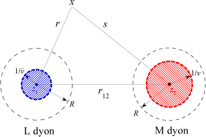
Figure 4: Three regions of integration for well separated dyons.

Although there is no principle difficulty in doing all calculations exactly for the whole caloron moduli space, at some point we loose the capacity of performing analytical calculations for the simple reason that expressions become too long, and so far we have not been able to put them into a manageable form in a general case. Therefore, we have to adopt a more subtle attitude. First of all we restrict ourselves to the part of the moduli space corresponding to large separations between dyons ($r_{12}\gg 1$). Physically, it seems to be the most interesting case, see section I. Furthermore, at the first stage we take $r_{12}{\rm v},r_{12}\overline{{\rm v}}\gg 1$, meaning that the dyons are well separated and do not overlap since the separation is then much bigger than the core sizes, see Figs. 1,3 (left). In this case, the vacuum current $J_{\mu}$ (20) becomes that of single dyons inside the spheres of some radius R surrounding the dyon centers, such that $\frac{1}{{\rm v}},\frac{1}{\overline{{\rm v}}}\ll R\ll r_{12}$, and outside these spheres it can be computed analytically with exponential precision, in correspondence with subsection II.B, see Fig. 4. Adding up the contributions of the regions near two dyons and of the far-away region, we get $d{\rm Det}(-D^{2})/d{\rm v}$ for well-separated dyons. Integrating it over ${\rm v}$ we obtain the determinant itself up to a constant and possible $1/r_{12}$ terms.

This is already an interesting result by itself, however, we would like to compute the constant, which can be done by matching our calculation with that for the trivial caloron at ${\rm v}=0$. It means that we have to extend the domain of applicability to $r_{12}{\rm v}={\cal O}(1)$ (or $r_{12}\overline{{\rm v}}={\cal O}(1)$) implying overlapping dyons, presented in Figs. 1,3 (right). To make this extension, we ‘guess’ the analytical expression which would interpolate between $r_{12}{\rm v}\gg 1$ where the determinant is already computed and $r_{12}{\rm v}\ll 1$ where matching with the Gross–Pisarski–Yaffe (GPY) calculation GPY can be performed. At this point it becomes very helpful that we possess the exact vacuum current for the caloron, which, although too long to be put on paper, is nevertheless affordable for numerical evaluation (and can be provided on request). We check our analytical ‘guess’ to the accuracy better than one millionth. In this way we obtain the determinant up to an overall constant factor for any ${\rm v},\overline{{\rm v}}$ with the only restriction that $r_{12}\gg 1$. This constant factor is then read off from the GPY calculation GPY .

Finally, we compute the $1/r_{12}$ and $\log r_{12}/r_{12}$ corrections in the ${\rm Det}(-D^{2})$, which turn out to be quite non-trivial.

IV Det${\bf(-D^{2})}$ for well separated dyons

The L,M dyon cores have the sizes $\frac{1}{\overline{{\rm v}}}$ and $\frac{1}{{\rm v}}$, respectively, and in this section we consider the case of well-separated dyons, meaning that the distance between the two centers is much greater than the core sizes, $r_{12}\gg\frac{1}{{\rm v}},\;\frac{1}{\overline{{\rm v}}}$. This situation is depicted in Figs. 1,3 (left). The two dyons are static in time, so that $\partial\,\log{\rm Det}(-D^{2})/\partial{\rm v}$ (19) becomes an integral over $3d$ space, times $1/T$ set to unity. We divide the $3d$ volume into to three regions (Fig. 4): i) a ball of radius R centered at the center of the M dyon, ii) a ball of radius R centered at the L dyon, iii) the rest of the space, with two balls removed. The radius R is chosen such that it is much larger than the dyon cores but much less than the separation: $r_{12}\gg R\gg\frac{1}{{\rm v}},\;\frac{1}{\overline{{\rm v}}}$. Summing up the contributions from the three regions of space, we are satisfied to observe that the result does not depend on the intermediate radius $R$.

IV.1 Det${\bf(-D^{2})}$ for a single dyon

In region i) the KvBLL caloron field can be approximated by the M dyon field (13), and the vacuum current by that inside a single dyon, both with the ${\cal O}(1/r_{12})$ accuracy. We make a more precise calculation, including the ${\cal O}(1/r_{12})$ terms, in section V. The single-dyon vacuum current is calculated in Appendix C. Adding up the three parts of the vacuum current denoted there as $J_{\mu}^{\rm s,r,m}$ we obtain the full isospin-1 vacuum current (in the ‘stringy’ gauge)

$$J_{r} = 0,$$

$$J_{\phi} = -\frac{i{\rm v}(\sin(\phi)T_{2}+\cos(\phi)T_{1})(1-s{\rm v}\coth(s{\rm v}))^{2}}{24\pi^{2}s^{2}\sinh(s{\rm v})},$$

$$J_{\theta} = -\frac{i{\rm v}(\sin(\phi)T_{1}-\cos(\phi)T_{2})(1-s{\rm v}\coth(s{\rm v}))^{2}}{24\pi^{2}s^{2}\sinh(s{\rm v})},$$

$$J_{4} = -iT_{3}\left[\frac{(1-s{\rm v}\coth(s{\rm v}))^{3}}{6\pi^{2}s^{3}}+\frac{1-s{\rm v}\coth(s{\rm v})}{3s}+\frac{\coth(s{\rm v})(1-s{\rm v}\coth(s{\rm v}))^{2}}{2\pi s^{2}}\right]\;,$$

where ${(T_{c})}^{ab}\equiv i\varepsilon^{acb}$ are the isospin-1 generators. We contract $J_{\mu}$ (IV.1) with $dA_{\mu}/d{\rm v}$ from eq.(13) according to eq.(19). After taking the matrix trace, the integrand in eq.(19) becomes spherically symmetric:

$${\rm Tr}\left[\partial_{\rm v}A_{\mu}J_{\mu}\right] = \frac{2}{3s}\left(\coth(s{\rm v})-s{\rm v}+\frac{s{\rm v}\left(s{\rm v}\coth(s{\rm v})-2\right)}{\sinh^{2}(s{\rm v})}\right)$$ (23)

$$- \frac{{\left(s{\rm v}\coth(s{\rm v})-1\right)}^{3}\left(\sinh(2s{\rm v})-3s{\rm v}\right)}{6\pi^{2}\sinh^{2}(s{\rm v})s^{3}}+\frac{{\left(s{\rm v}\coth(s{\rm v})-1\right)}^{2}\left(\sinh(2s{\rm v})-2s{\rm v}\right)}{2\pi\sinh^{2}(s{\rm v})\tanh(s{\rm v})s^{2}};$$

It has to be integrated over the spherical box of radius R. Fortunately, we are able to perform the integration analytically. The result for the M dyon is

$$\frac{\partial\,\log\,{\rm Det}(-D^{2}[{\rm M\,dyon}])}{\partial{\rm v}} = -\int_{0}^{R}\!ds\,{\rm Tr}\left[\partial_{\rm v}A_{\mu}J_{\mu}\right]4\pi s^{2}=-\frac{24(\gamma_{E}-\log\pi)+53+\frac{2}{3}\pi^{2}}{18\pi}+\frac{1}{{\rm v}}$$ (24)

$$+ \frac{4\pi R^{3}}{3}P^{\prime}({\rm v})-2\pi R^{2}\,P^{\prime\prime}({\rm v})+2\pi R\,P^{\prime\prime\prime}({\rm v})-\frac{4}{3\pi}\log(R{\rm v}).$$

As we see, it is badly infrared divergent, as it depends on the box radius $R$. Here $P(q)$ is the potential energy (see eq.(2))

$$P(q)=\left[\frac{\pi^{2}}{12}\left(\frac{q}{\pi}-2\right)^{2}\left(\frac{q}{\pi}\right)^{2}\right],\qquad P^{\prime}(q)=\frac{1}{3\pi^{2}}q(\pi-q)(2\pi-q),$$

$$P^{\prime\prime}(q)=\frac{1}{3\pi^{2}}(3q^{2}-6\pi q+2\pi^{2}),\qquad P^{\prime\prime\prime}(q)=\frac{2}{\pi^{2}}(q-\pi),\qquad P^{\rm IV}(q)=\frac{2}{\pi^{2}}.$$

The IR-divergent terms arise from the asymptotics of the integrand. Neglecting exponentially small terms $e^{-s{\rm v}}$ in eq.(23) we have

$$-{\rm Tr}\left[\partial_{\rm v}A_{\mu}J_{\mu}\right] \simeq -4\left[\frac{(1-s{\rm v})^{3}}{12\pi^{2}s^{3}}+\frac{(1-s{\rm v})^{2}}{4\pi s^{2}}+\frac{1-s{\rm v}}{6s}\right]$$

$$=P^{\prime}\left({\rm v}-\frac{1}{s}\right)=P^{\prime}({\rm v})-P^{\prime\prime}({\rm v})\frac{1}{s}+\frac{1}{2}P^{\prime\prime\prime}({\rm v})\frac{1}{s^{2}}-\frac{1}{6}P^{\rm IV}({\rm v})\frac{1}{s^{3}}.$$

Integrating it over the sphere of radius R one gets the IR-divergent terms (the second line in eq.(24)).

The fact that the IR-divergent part of $d{\rm Det}(-D^{2})/d{\rm v}$ is directly related to the potential energy $P(A_{4})$ is not accidental. At large distances the field of the dyon becomes a slowly varying Coulomb field, see eq.(14). Therefore, the determinant can be generically expanded in the covariant derivatives of the background field DO ; RA with the potential energy $P(A_{4})$ being its leading zero-derivative term. The nontrivial fact, however, is that with exponential precision the vacuum current is related to the variation of solely the leading term in the covariant derivative expansion of the effective action with no contribution from any of the subleading terms. This is a specific property of self-dual fields, and we observe it also in the following subsection.

IV.2 Contribution from the far-away region

We now compute the contribution to $\partial{\rm Det}(-D^{2})/\partial{\rm v}$ from the region of space far away from both dyon centers. With exponential accuracy (meaning neglecting terms of the order of $e^{-r\overline{{\rm v}}}$ and $e^{-s{\rm v}}$) the KvBLL caloron field is given by eqs.(17,18), and only the $A_{4}$ component depends (trivially) on ${\rm v}$. The caloron vacuum current with the same exponential accuracy is calculated in Appendix D. Combining the results given by eqs.(180,181) and eqs.(183,184) we see that $J_{\varphi}=0$ and for $J_{4}$ we have

$$J_{4} = \frac{iT_{3}}{2}\left\{\left[\frac{1}{3\pi^{2}}\left(\frac{1}{r}-\frac{1}{s}\right)^{3}-\frac{1}{\pi}\left(\frac{1}{r}-\frac{1}{s}\right)^{2}+\frac{2}{3}\left(\frac{1}{r}-\frac{1}{s}\right)\right]+\left[\frac{4}{\pi}\left(\frac{1}{r}-\frac{1}{s}\right)^{2}-8\left(\frac{1}{r}-\frac{1}{s}\right)+\frac{8\pi}{3}\right]\omega\right.$$ (25)

$$+ \left.\left[16\left(\frac{1}{r}-\frac{1}{s}\right)-16\pi\right]\omega^{2}+\frac{64\pi}{3}\,\omega^{3}\right\}\,.$$

We remind the reader that $r,s$ are distances from M,L dyon centers $\vec{z}_{1,2}$ and that $\omega={\rm v}/(4\pi)$. It is interesting that the separation $r_{12}=|z_{1}-z_{2}|$ does not appear explicitly in the current. Moreover, it can be again written through the potential energy $P(A_{4})$:

$$J_{4}=\frac{1}{2}iT_{3}\left.P^{\prime}(q)\right|_{q={\rm v}+1/r-1/s}\,.$$ (26)

Therefore, in the far-away region one obtains

$$-{\rm Tr}\left[\partial_{\rm v}A_{\mu}J_{\mu}\right]=P^{\prime}\left({\rm v}+\frac{1}{r}-\frac{1}{s}\right)\;.$$ (27)

We have now to integrate eq.(27) over the whole $3d$ space with two spheres of radius $R$ surrounding the dyon centers removed:

$$-\int\!d^{4}x\,{\rm Tr}\left[\partial_{\rm v}A_{\mu}J_{\mu}\right] = \int\!d^{3}x\,P^{\prime}\left({\rm v}+\frac{1}{r}-\frac{1}{s}\right)$$

$$= P^{\prime}({\rm v})\!\int\!d^{3}x+P^{\prime\prime}({\rm v})\!\int\!\!d^{3}x\left(\frac{1}{r}-\frac{1}{s}\right)+\frac{1}{2}P^{\prime\prime\prime}({\rm v})\!\int\!\!d^{3}x\left(\frac{1}{r}-\frac{1}{s}\right)^{2}+\frac{1}{6}P^{\rm IV}({\rm v})\!\int\!\!d^{3}x\left(\frac{1}{r}-\frac{1}{s}\right)^{3}.$$

The first integral in eq.(IV.2) is the $3d$ volume $V$, minus the volume of two spheres, $V-2\frac{4\pi}{3}R^{3}$. The second integral is zero by symmetry between the two centers, and so is the last one. The only non-trivial integral is

$$\int\!d^{3}x\,\left(\frac{1}{r}-\frac{1}{s}\right)^{2}=4\pi r_{12}-8\pi R+{\cal O}\left(\frac{R^{2}}{r_{12}}\right).$$ (29)

Therefore, the contribution from the region far from both dyon centers is

$$\left.\frac{\partial\,\log\,{\rm Det}(-D^{2})}{\partial{\rm v}}\right|_{\rm far}=P^{\prime}({\rm v})\left(V-2\frac{4\pi}{3}R^{3}\right)+\frac{1}{2}P^{\prime\prime\prime}({\rm v})\left(4\pi r_{12}-8\pi R\right).$$ (30)

IV.3 Combining all three regions

We now add up the contributions to $\partial\log\,{\rm Det}(-D^{2})/\partial{\rm v}$ from the regions surrounding the two dyons and from the far-away region. Since the contribution of the L dyon is the same as that of the M dyon with the replacement ${\rm v}\to\overline{{\rm v}}$ and since $\partial/\partial{\rm v}=-\partial/\partial\overline{{\rm v}}$, when adding up contributions of L,M core regions we have to antisymmetrize in ${\rm v}\leftrightarrow\overline{{\rm v}}$. It should be noted that $P({\rm v})$ and $P^{\prime\prime}({\rm v})$ are symmetric under this interchange, while $P^{\prime}({\rm v})$ and $P^{\prime\prime\prime}({\rm v})$ are antisymmetric. Therefore, the combined contribution of both cores is, from eq.(24),

$$\left.\frac{\partial\,\log\,{\rm Det}(-D^{2})}{\partial{\rm v}}\right|_{\rm cores}=2P^{\prime}({\rm v})\frac{4\pi}{3}R^{3}+\frac{1}{2}P^{\prime\prime\prime}({\rm v})\,8\pi R+\frac{1}{{\rm v}}-\frac{1}{\overline{{\rm v}}}-\frac{4}{3\pi}\ln\left(\frac{{\rm v}}{\overline{{\rm v}}}\right).$$ (31)

Adding it up with the contribution from the far-away region, eq.(30), we obtain the final result which is independent of the intermediate radius $R$ used to separate the regions:

$$\frac{\partial\,\log\,{\rm Det}(-D^{2})}{\partial{\rm v}}=P^{\prime}({\rm v})\,V+P^{\prime\prime\prime}({\rm v})\,2\pi r_{12}+\frac{1}{{\rm v}}-\frac{1}{\overline{{\rm v}}}-\frac{4}{3\pi}\ln\left(\frac{{\rm v}}{\overline{{\rm v}}}\right).$$ (32)

This equation can be easily integrated over ${\rm v}$ up to a constant which in fact can be a function of the separation $r_{12}$:

$$\log\,{\rm Det}(-D^{2})=P({\rm v})\,V+P^{\prime\prime}({\rm v})\,2\pi r_{12}+\left(\!1-\frac{4{\rm v}}{3\pi}\!\right)\log({\rm v})+\left(\!1-\frac{4\overline{{\rm v}}}{3\pi}\!\right)\log(\overline{{\rm v}})+f(r_{12})\;.$$ (33)

Since in the above calculation of the determinant for well-separated dyons we have neglected the Coulomb field of one dyon inside the core region of the other, we expect that the unknown function $f(r_{12})={\cal O}(1/r_{12})+c$, where $c$ is the true integration constant. Our next aim will be to find it. The ${\cal O}(1/r_{12})$ corrections will be found later.

V Matching with the determinant with trivial holonomy

To find the integration constant, one needs to know the value of the determinant at ${\rm v}\!=\!0$ (or $\overline{{\rm v}}\!=\!0$) where the KvBLL caloron with non-trivial holonomy reduces to the Harrington–Shepard caloron with a trivial one and for which the determinant has been computed by GPY GPY . Before we match our determinant at ${\rm v}\!\neq\!0$ with that at ${\rm v}\!=\!0$ let us recall the GPY result.

V.1 Det${\bf(-D^{2})}$ at ${\rm v}=0$

The ${\rm v}\!=\!0$ periodic instanton is traditionally parameterized by the instanton size $\rho$. It is known Rossi ; GPY that the periodic instanton can be viewed as a mix of two BPS monopoles one of which has an infinite size. It becomes especially clear in the KvBLL construction KvB ; LL where the size of one of the dyons becomes infinite as ${\rm v}\to 0$, see section II. Despite one dyon being infinitely large, one can still continue to parametrize a caloron by the distance $r_{12}$ between dyon centers, with $\rho=\sqrt{r_{12}/\pi}$. Since our determinant (33) is given in terms of $r_{12}$ we have first of all to rewrite the GPY determinant in terms of $r_{12}$, too. Actually, GPY have interpolated the determinant in the whole range of $\rho$ (hence $r_{12}$) but we shall be interested only in the limit $r_{12}\gg 1$. In this range the GPY result reads:

$$\left.\log{\rm Det}(-D^{2})\right|_{{\rm v}=0,\;T=1} = \left.\log{\rm Det}(-D^{2})\right|_{{\rm v}=0,\;T=0}+\frac{4}{3}\pi r_{12}-\frac{4}{3}\log r_{12}+c_{0}+{\cal O}\left(\frac{1}{r_{12}}\right),$$ (34)

$$c_{0} = \frac{8}{9}-\frac{8\,\gamma_{E}}{3}-\frac{2\,\pi^{2}}{27}+\frac{4\,\log\pi}{3}.$$

We have made here a small improvement as compared to ref. GPY , namely i) we have checked that the correction is of the order of $1/r_{12}$ basing on an intermediate exact formula, ii) we have also managed to get an exact analytical expression for the constant.

The zero-temperature determinant is that for the standard BPST instanton tHooft ; Bernard :

$$\left.\log{\rm Det}(-D^{2})\right|_{{\rm v}=0,\;T=0} = \frac{2}{3}\log\mu+\frac{1}{3}\log\left(\frac{r_{12}}{\pi}\right)+\alpha(1),$$ (35)

$$\alpha(1) = \frac{2\gamma_{E}}{3}-\frac{16}{9}+\frac{\log 2}{3}+\frac{2\log(2\pi)}{3}-\frac{4\zeta^{\prime}(2)}{{\pi}^{2}}\;,$$ (36)

where it is implied that the determinant is regularized by the Pauli–Villars method and $\mu$ is the Pauli–Villars mass, see section VI.A. Combining eqs.(34,35) one obtains

$$\left.\log{\rm Det}[-D^{2}]\right|_{{\rm v}=0,\;T=1}=\frac{4}{3}\pi r_{12}-\log r_{12}+\frac{2}{3}\log\mu+c_{1}+{\cal O}\left(\frac{1}{r_{12}}\right),$$ (37)

where

$$c_{1}=\log 2+\frac{5}{3}\log\pi-\frac{8}{9}-2\,\gamma_{E}-\frac{2\,\pi^{2}}{27}-\frac{4\,\zeta^{\prime}(2)}{{\pi}^{2}}=0.206602292859\,.$$ (38)

We notice that $P({\rm v})\to 0$ and $P^{\prime\prime}({\rm v})\to\frac{2}{3}$ at ${\rm v}\to 0$, therefore the first two terms in eq.(33) become exactly equal to the first term in eq.(37). At the same time, the last two terms in eq.(33) become $\log{\rm v}-\frac{5}{3}\log(2\pi)+c$ which is formally singular at ${\rm v}\to 0$ and does not match the $-\!\log r_{12}$ in eq.(37). The reason is, eq.(33) has been derived assuming $r_{12}\gg\frac{1}{{\rm v}},\frac{1}{\overline{{\rm v}}}$ and one cannot take the limit ${\rm v}\to 0$ in that expression without taking simultaneously $r_{12}\to\infty$. In order to match the determinant at ${\rm v}=0$ one needs to extend eq.(33) to arbitrary values of ${\rm v}r_{12}$. As we shall see, it will be important for the matching that $\log r_{12}$ has the coefficient $-1$.

V.2 Extending the result to arbitrary values of ${\rm v}r_{12}$

Let us take a fixed but large value of the dyon separation $r_{12}\gg 1$ such that both eq.(33) and eq.(37) are valid. Actually, our aim is to integrate the exact expression for the derivative of the determinant

$$\partial_{\rm v}\log{\rm Det}(-D^{2})=\int\wp(x)d^{4}x,\qquad\wp(x)\equiv-{\rm Tr}\left[\partial_{\rm v}A_{\mu}J^{\mu}(x,x|A)\right],$$ (39)

from ${\rm v}=0$ where the determinant is given by eq.(37), to some small value of ${\rm v}\ll 1$ (but such that ${\rm v}r_{12}\gg 1$) where eq.(33) becomes valid. We shall parametrize this ${\rm v}$ as ${\rm v}=k/r_{12}\ll 1$ with $k\gg 1$. The result of the integration over ${\rm v}$ must be equal to the difference between the right hand sides of eqs.(33,37). We write it as

$$\int_{0}^{\frac{k}{r_{12}}}\!d{\rm v}\!\int\!d^{4}x\,\wp(x)=V\left[P\left(\!\frac{k}{r_{12}}\!\right)-P(0)\right]+2\pi r_{12}\left[P^{\prime\prime}\left(\!\frac{k}{r_{12}}\!\right)-P^{\prime\prime}(0)\right]+\log(k)+c-\frac{5}{3}\log(2\pi)-c_{1}-\frac{2}{3}\log\mu+{\cal O}\left(\!\frac{k}{r_{12}}\!\right).$$ (40)

Notice that $\log r_{12}$ has cancelled in the difference in the r.h.s. We denote

$$c_{2}\equiv c-c_{1}-\frac{2}{3}\log\mu-\frac{5}{3}\log(2\pi)\;.$$ (41)

We know that the first two terms in eq.(40) come from far asymptotics. Denoting by $\bar{\wp}$ our $\wp$ with subtracted asymptotic terms we have

$$\int_{0}^{\frac{k}{r_{12}}}d{\rm v}\int\!d^{4}x\,\bar{\wp}(x)=\log k+c_{2}+{\cal O}\left(\frac{1}{r_{12}}\right)\;.$$ (42)

In this integration we are in the domain $1/{\rm v}\gg 1$ and $r_{12}\gg 1$ and we can simplify the integrand dropping terms which are small in this domain. At this point it will be convenient to restore temporarily the temperature dependence. With $\beta\equiv 1/T$ our domain of interest is $1/{\rm v}\gg\beta$ and $r_{12}\gg\beta$. Therefore we are in the small-$\beta$ domain and can expand $\bar{\wp}$ in series with respect to $\beta$:

$$\bar{\wp}=\frac{1}{\beta^{2}}\wp_{0}+\frac{1}{\beta}\wp_{1}+{\cal O}(\beta^{0})\;.$$ (43)

As we shall see in a moment, only the first two terms are not small in this domain and we need to know only them to compute $c_{2}$. It is a great simplification because $\wp_{0,1}$ do not contain terms proportional to $e^{-\overline{{\rm v}}r}$ since $\overline{{\rm v}}=2\pi T-{\rm v}\to\infty$ at $\beta\to 0$, and what is left is time independent. Moreover, what is left after we neglect exponentially small terms are homogeneous functions of $r,s,r_{12},{\rm v}$ and we can turn to the dimensionless variables:

$$\wp_{0}(r,s,r_{12},{\rm v})=\frac{1}{r_{12}}\widetilde{\wp}_{0}\left(\frac{r}{r_{12}},\frac{s}{r_{12}},\frac{{\rm v}}{r_{12}}\right),$$

$$\wp_{1}(r,s,r_{12},{\rm v})=\frac{1}{r_{12}^{2}}\widetilde{\wp}_{1}\left(\frac{r}{r_{12}},\frac{s}{r_{12}},\frac{{\rm v}}{r_{12}}\right)\;.$$

We rewrite the l.h.s. of eq.(42) in terms of the new quantities:

$$\int\!d^{4}x\,\bar{\wp}(x)=\frac{r_{12}^{2}}{\beta}\int\!d^{3}\tilde{x}\,\widetilde{\wp}_{0}+r_{12}\int\!d^{3}\tilde{x}\,\widetilde{\wp}_{1}+{\cal O}(\beta)\;,$$ (44)

where $\tilde{x}=x/r_{12}$ is dimensionless. We see that it is indeed sufficient to take just the first two terms in the expansion (43) at $\beta\to 0$. The integration measure can be written in terms of the dimensionless variables $\tilde{r}=r/r_{12},\,\tilde{s}=s/r_{12}$ as

$$d^{3}\tilde{x}=2\pi\,\tilde{r}d\tilde{r}\,\tilde{s}\,d\tilde{s}\;,$$ (45)

where $\tilde{r}$ and $\tilde{s}$ are constrained by the triangle inequalities $\tilde{r}\!+\!\tilde{s}\!<\!1$, $\tilde{r}\!+\!1\!<\!\tilde{s}$ and $\tilde{s}\!+\!1\!<\!\tilde{r}$, and we have integrated over the azimuth angle.

We have now to use the exact vacuum current to compute $\int\tilde{\wp}_{0,1}$. First, it turns out that the first integral in eq.(44) is zero. This is good news because had it been nonzero, eq.(42) could not be right as its r.h.s. has no dependence on $r_{12}$ other than possible $1/r_{12}$ terms. Second, we have noticed that the second integral in eq.(44) is in fact

$$\int\!d^{3}\tilde{x}\,\widetilde{\wp}_{1}=\frac{1}{{\rm v}r_{12}+1}\,.$$ (46)

Unfortunately, we were not able to verify it analytically but we checked numerically that it holds with the precision of a few units of $10^{-7}$ in the range of ${\rm v}r_{12}$ between 0 and 15. Combining eqs.(44,46) we obtain for the l.h.s. of eq.(42)

$$\int_{0}^{\frac{k}{r_{12}}}d{\rm v}\int\!d^{4}x\,\bar{\wp}(x)=r_{12}\int_{0}^{\!\frac{k}{r_{12}}}\frac{d{\rm v}}{{\rm v}r_{12}+1}=\log(k+1)=\log k+{\cal O}\left(\frac{1}{k}\right).$$

Therefore, we reproduce the r.h.s. of eq.(42) and in addition find that $c_{2}=0$.

Eq.(46) is sufficient to extend the result for the determinant (33) valid at ${\rm v}r_{12}\gg 1$ to arbitrary values of ${\rm v}r_{12}$, provided $r_{12}\gg 1$ (the extension to arbitrary values of $\overline{{\rm v}}r_{12}$ is obtained by symmetry ${\rm v}\leftrightarrow\overline{{\rm v}}$). The final result for the determinant to the $1/r_{12}$ accuracy is

$$\log{\rm Det}[\!-\!D^{2}] = VP({\rm v})+2\pi P^{\prime\prime}({\rm v})\,r_{12}+\left(1-\frac{4{\rm v}}{3\pi}\right)\log\left({\rm v}r_{12}+1\right)+\left(1-\frac{4\overline{{\rm v}}}{3\pi}\right)\log\left(\overline{{\rm v}}r_{12}+1\right)$$ (47)

$$+ \frac{2}{3}\log(\mu r_{12})+c_{1}+\frac{5}{3}\log(2\pi)+{\cal O}\left(\frac{1}{r_{12}}\right)$$

where $\mu$ is the UV cutoff and the numerical constant $c_{1}$ is given by eq.(38). This expression is finite at ${\rm v}\to 0,\,\overline{{\rm v}}\to 0$ and coincides with the GPY result (37) in these limits. At ${\rm v}r_{12}\gg 1$ we restore the previous result, eq.(33), but now with the integration constant fixed: $c=\frac{2}{3}\log\mu+\frac{5}{3}\log(2\pi)+c_{1}$. Eq.(47) is valid for any holonomy, i.e. for ${\rm v},\overline{{\rm v}}\in[0,2\pi]$, and the only restriction on its applicability is the condition that the dyon separation is large, $r_{12}\gg 1$.

V.3 $1/r_{12}$ corrections

Eq.(47) can be expanded in inverse powers of ${\rm v}r_{12},\overline{{\rm v}}r_{12}$, which gives $1/({\rm v}r_{12}),\;1/(\overline{{\rm v}}r_{12})$ (and higher) corrections; however, there are other $1/r_{12}$ corrections which are not accompanied by the $1/{\rm v},\;1/\overline{{\rm v}}$ factors: the aim of this subsection is to find them using the exact vacuum current.

To this end, we again consider the case $r_{12}\gg\frac{1}{{\rm v}},\,\frac{1}{\overline{{\rm v}}}$ such that one can split the integration over $3d$ space into three regions shown in Fig. 4. In the far-away region one can use the same vacuum current (25) as it has an exponential precision with respect to the distances to both dyons. In the core regions, however, it is now insufficient to neglect completely the field of the other dyon, as we did in section IV looking for the leading order. Since we are now after the $1/r_{12}$ corrections, we have to use the exact field and the exact vacuum current of the caloron but we can neglect the exponentially small terms in their separation.

Another modification with respect to section IV is that we find it more useful this time to choose $r_{12}$ as the parameter $\cal P$ in eq.(19). We shall compute the $1/r_{12}^{2}$ terms in $\partial{\rm Det}(\!-\!D^{2})/\partial r_{12}$ and then restore the determinant itself since the limit of $r_{12}\to\infty$ is already known. Let us define how the KvBLL field depends on $r_{12}$. As seen from eq.(7) the KvBLL field is a function of $r,\;s,\;{\rm v},\;r_{12}$ only. We define the change in the separation $r_{12}\to r_{12}+dr_{12}$ as the symmetric displacement of each monopole center by $\pm dr_{12}/2$. It corresponds to

$$\frac{\partial r}{\partial r_{12}}=\frac{r_{12}^{2}+r^{2}-s^{2}}{4r_{12}r},\qquad\frac{\partial s}{\partial r_{12}}=\frac{r_{12}^{2}+s^{2}-r^{2}}{4r_{12}s}.$$ (48)

We shall use the definition (48) to compute the derivative of the caloron field (7) with respect to $r_{12}$.

Let us start from the $M$-monopole core region. To get the $1/r_{12}$ correction to the determinant we need to compute its derivative in the $1/r_{12}^{2}$ order and expand correspondingly the caloron field and the vacuum current to this order. Wherever the distance $r$ from the far-away L dyon appears in the equations, we replace it by $r=(r_{12}^{2}+2sr_{12}\cos\theta+s^{2})^{1/2}$ where $s$ is the distance from the M-dyon and $\theta$ is the polar angle seen from the M-dyon center. Expanding in inverse powers of $r_{12}$ we get coefficients that are functions of $s,\cos\theta$. One can easily integrate over $\theta$ as the integration measure in spherical coordinates is $2\pi s^{2}ds\;d\cos\theta$. We leave out the intermediate equations and give only the end result for the integrand in eq.(19). After integrating over $\cos\theta$ we obtain the following contribution from the core region of the M monopole:

$$\left.\frac{\partial{\rm Det}(\!-\!D^{2})}{\partial r_{12}}\right|_{\rm M\;dyon\;core}=-\frac{1}{r_{12}^{2}}\int_{0}^{R}\!I_{1/r_{12}^{2}}16\pi s^{2}ds+{\cal O}\left(\frac{1}{r_{12}^{3}}\right),$$ (49)

where $I_{1/r_{12}^{2}}$ reads

$$I_{1/r_{12}^{2}}=-\frac{\coth(s{\rm v})}{12\pi^{2}s^{3}}-\frac{\coth(s{\rm v})}{9s}-\frac{s{\rm v}^{2}\coth(s{\rm v}){{\rm csch}(s{\rm v})}^{2}}{36}-\frac{s^{2}{\rm v}^{3}\left(2+\cosh(2s{\rm v})\right){{\rm csch}(s{\rm v})}^{4}}{72}$$

$$+\frac{{\rm v}\left(-61+3\cosh(2s{\rm v})+4\cosh(4s{\rm v})\right)\coth(s{\rm v}){{\rm csch}(s{\rm v})}^{4}}{96\pi s}-\frac{{\rm v}^{2}\left(37+23\cosh(2s{\rm v})+4\cosh(4s{\rm v})\right)\coth(s{\rm v}){{\rm csch}(s{\rm v})}^{4}}{192\pi^{2}s}$$

$$+\frac{s^{2}{\rm v}^{4}\left(4+\cosh(2s{\rm v})\right){\coth(s{\rm v})}^{2}{{\rm csch}(s{\rm v})}^{4}}{48\pi}-\frac{s{\rm v}^{3}\left(54\cosh(s{\rm v})+17\cosh(3s{\rm v})+\cosh(5s{\rm v})\right){{\rm csch}(s{\rm v})}^{7}}{384\pi}$$

$$+\frac{s{\rm v}^{4}\left(-406\cosh(s{\rm v})-81\cosh(3s{\rm v})+7\cosh(5s{\rm v})\right){{\rm csch}(s{\rm v})}^{7}}{2304\pi^{2}}-\frac{s^{2}{\rm v}^{5}\left(-24-33\cosh(2s{\rm v})+\cosh(6s{\rm v})\right){{\rm csch}(s{\rm v})}^{8}}{1536\pi^{2}}$$

$$+{\rm v}\frac{6+13{{\rm csch}(s{\rm v})}^{2}}{72}+\frac{-10-5{{\rm csch}(s{\rm v})}^{2}+9{{\rm csch}(s{\rm v})}^{4}}{48\pi s^{2}}+{\rm v}\frac{40+65{{\rm csch}(s{\rm v})}^{2}+19{{\rm csch}(s{\rm v})}^{4}}{192\pi^{2}s^{2}}$$

$$+{\rm v}^{2}\frac{-6-20{{\rm csch}(s{\rm v})}^{2}+9{{\rm csch}(s{\rm v})}^{4}+27{{\rm csch}(s{\rm v})}^{6}}{48\pi}+{\rm v}^{3}\frac{24+98{{\rm csch}(s{\rm v})}^{2}+285{{\rm csch}(s{\rm v})}^{4}+234{{\rm csch}(s{\rm v})}^{6}}{576\pi^{2}}\,.$$ (50)

Fortunately we are able to integrate this function analytically:

$$\int_{0}^{R}\!\!I_{1/r_{12}^{2}}16\pi s^{2}ds=\frac{1}{{\rm v}}-\frac{\pi^{2}+36\gamma_{E}+69}{27\pi}+\frac{2{\rm v}({\rm v}^{2}-3\pi{\rm v}+2\pi^{2})}{9\pi}R^{3}+\frac{4(6{\rm v}\pi-2\pi^{2}-3{\rm v}^{2})}{9\pi}R^{2}+\frac{10({\rm v}-\pi)}{3\pi}R-\frac{4\log(R{\rm v}/\pi)}{3\pi}.$$ (51)

For the $L$ monopole core contribution one has to replace ${\rm v}$ by $\overline{{\rm v}}$. Adding together contributions from L,M monopole cores we have

$$\left.\frac{\partial{\rm Det}(\!-\!D^{2})}{\partial r_{12}}\right|_{\rm cores}=-\frac{1}{r_{12}^{2}}\left[\frac{1}{{\rm v}}+\frac{1}{\overline{{\rm v}}}-2\frac{\pi^{2}+36\gamma_{E}+69}{27\pi}-\frac{8}{9\pi}(3{\rm v}^{2}-6\pi{\rm v}+2\pi^{2})R^{2}-\frac{4\log(R^{2}{\rm v}\overline{{\rm v}}/\pi^{2})}{3\pi}\right].$$ (52)

Now let us turn to the far-away region. Recalling eq.(26) we realize that the contribution of this region is determined by the potential energy:

$$\left.\frac{\partial{\rm Det}(\!-\!D^{2})}{\partial r_{12}}\right|_{\rm far}=\int\!d^{3}x\,\partial_{r_{12}}P\left({\rm v}+\frac{1}{r}-\frac{1}{s}\right)=\frac{1}{2}P^{\prime\prime}({\rm v})\int\!d^{3}x\,\partial_{r_{12}}\left(\frac{1}{r}-\frac{1}{s}\right)^{2}+\frac{1}{24}P^{\rm IV}({\rm v})\int\!d^{3}x\,\partial_{r_{12}}\left(\frac{1}{r}-\frac{1}{s}\right)^{4}.$$

The integration region is the $3d$ volume with two balls of radius $R$ removed. We use

$$\int\!d^{3}x\,\partial_{r_{12}}\left(\frac{1}{r}-\frac{1}{s}\right)^{2}=4\pi-\frac{16\pi R^{2}}{3r_{12}^{2}},\qquad\int\!d^{3}x\,\partial_{r_{12}}\left(\frac{1}{r}-\frac{1}{s}\right)^{4}=\frac{2\pi}{3r_{12}^{2}}\left[48\log\left(\frac{r_{12}}{R}\right)-9\pi^{2}+8\right].$$ (53)

Adding up all three contributions we see that the region separation radius $R$ gets cancelled (as it should), and we get

$$\partial_{r_{12}}\log{\rm Det}(-D^{2})=2\pi P^{\prime\prime}({\rm v})+\frac{1}{r_{12}^{2}}\left[\frac{4}{3\pi}\log\left(\frac{{\rm v}\overline{{\rm v}}\,r_{12}^{2}}{\pi^{2}}\right)-\frac{1}{{\rm v}}-\frac{1}{\overline{{\rm v}}}+\frac{50}{9\pi}+\frac{8\gamma_{E}}{3\pi}-\frac{23\pi}{54}\right]$$ (54)

which can be easily integrated, with the result

$$\log{\rm Det}(-D^{2})=2\pi P^{\prime\prime}({\rm v})\,r_{12}+\frac{1}{r_{12}}\left[\frac{1}{{\rm v}}+\frac{1}{\overline{{\rm v}}}+\frac{23\pi}{54}-\frac{8\gamma_{E}}{3\pi}-\frac{74}{9\pi}-\frac{4}{3\pi}\log\left(\frac{{\rm v}\bar{\rm v}\,r_{12}^{2}}{\pi^{2}}\right)\right]+\bar{c}+{\cal O}\left(\frac{1}{r_{12}^{2}}\right)$$ (55)

where $\bar{c}$ is the integration constant that does not depend on $r_{12}$. Comparing eq.(55) with eq.(32) at $r_{12}\to\infty$ we conclude that

$$\bar{c}=V\,P({\rm v})+\frac{2}{3}\log\mu+\frac{3\pi-4{\rm v}}{3\pi}\log{\rm v}+\frac{3\pi-4\overline{{\rm v}}}{3\pi}\log\overline{{\rm v}}+\frac{5}{3}\log(2\pi)+c_{1}$$ (56)

and $c_{1}$ is given in eq.(38). We note that the leading correction, $\log r_{12}/r_{12}$, arises from the far-away region and is related to the potential energy, similar to the leading $r_{12}$ term. The terms proportional to $\frac{1}{{\rm v}}$ and $\frac{1}{\overline{{\rm v}}}$ can be extracted from expanding eq.(47) (which is an additional independent check of eq.(46)). In fact, eqs.(47) and (55) are complementary: eq.(47) sums up all powers of $\frac{1}{r_{12}{\rm v}},\,\frac{1}{r_{12}\overline{{\rm v}}}$ but misses $\frac{\log r_{12}}{r_{12}}$ and $\frac{1}{r_{12}}$ terms, whereas eq.(55) collects all terms of that order but misses higher powers of $\frac{1}{r_{12}{\rm v}},\,\frac{1}{r_{12}\overline{{\rm v}}}$.

VI Quantum weight of the KvBLL caloron

VI.1 Quantum weight of a Euclidean pseudoparticle: generalities

If a field configuration $\bar{A}_{\mu}$ is a solution of the Yang–Mills Euclidean equation of motion, $D_{\mu}F_{\mu\nu}=0$, its quantum weight is the contribution of the saddle point to the partition function

$${\cal Z}=\int DA_{\mu}\exp(-S[A]),\qquad S[A]=\frac{1}{4g^{2}}\int d^{4}x\;F_{\mu\nu}^{a}F_{\mu\nu}^{a}.$$ (57)

The general field over which one integrates in eq.(57) can be written as

$$A_{\mu}=\bar{A}_{\mu}+a_{\mu}$$ (58)

where $\bar{A}_{\mu}$ is the classical solution corresponding to the local minimum of the action and $a_{\mu}$ is the presumably small quantum oscillation about the solution. One expands the action around the minimum,

$$S[A]=S[\bar{A}]-\frac{1}{g^{2}}\int\!d^{4}x\,a_{\nu}^{a}D^{ab}_{\mu}(\bar{A})F^{b}_{\mu\nu}(\bar{A})+\frac{1}{2g^{2}}\int\!d^{4}x\,a_{\mu}^{a}\,W^{ab}_{\mu\nu}(\bar{A})\,a_{\nu}^{b}+{\cal O}(a^{3}),$$ (59)

where the linear term is in fact absent since $\bar{A}$ satisfies the equation of motion, and the quadratic form is

$$W_{\mu\nu}^{ab}(\bar{A}) = -D^{2}(\bar{A})^{ab}\delta_{\mu\nu}+(D_{\mu}D_{\nu})^{ab}(\bar{A})-2f^{acb}F^{c}_{\mu\nu}(\bar{A}),$$ (60)

$$D_{\mu}^{ab}(\bar{A}) = \partial_{\mu}\delta^{ab}+f^{acb}\bar{A}_{\mu}^{c}.$$ (61)

We have written the covariant derivative in the adjoint representation; the relation with the fundamental representation is given by $a_{\mu}=-ia_{\mu}^{a}t^{a},\;{\rm Tr}(t^{a}t^{b})=\frac{1}{2}\delta^{ab}$ and similarly for $F_{\mu\nu}$, etc. The 1-loop approximation to the quantum weight corresponds to evaluating eq.(57) in the Gaussian approximation in $a_{\mu}$, hence ${\cal O}(a^{3})$ terms in eq.(59) have been neglected.

The quadratic form (60) is highly degenerate since any fluctuation of the type $a_{\mu}^{a}=D_{\mu}^{ab}(\bar{A})\Lambda^{b}(x)$ corresponding to an infinitesimal gauge transformation of the saddle-point field $\bar{A}$, nullifies it. Therefore, one has to impose a gauge-fixing condition on $a_{\mu}$. The conventional choice is the background Lorenz gauge $D_{\mu}^{ab}(\bar{A})a_{\mu}^{b}=0$: with this condition imposed the operator $W$ simplifies as the second term in eq.(60) can be dropped. Fixing this gauge, however, brings in the Faddeev–Popov ghost determinant ${\rm Det}(-D^{2}(\bar{A}))$.

To define the path integral, one decomposes the fluctuation field in the complete set of the eigenfunctions of the quadratic form,

$$a_{\mu}^{a}(x)=\sum_{n}c_{n}\psi^{a}_{\mu\,n}(x),\qquad W^{ab}_{\mu\nu}\psi^{b}_{\nu\,n}=\lambda_{n}\psi^{b}_{\mu\,n},\qquad D^{ab}_{\mu}\psi^{b}_{\mu\,n}=0,$$ (62)

and implies that the path integral is understood as the integral over Fourier coefficients in the decomposition:

$$DA_{\mu}(x)=\prod_{n}\frac{dc_{n}}{\sqrt{2\pi}},$$ (63)

The quadratic form (60) has a finite number of zero modes related to the moduli space of the solution. Let the number of zero modes be $p$ (for a self-dual solution with topological charge one $p=4N$ for the $SU(N)$ gauge group CWS ). Let $\xi_{i},\,i=1...p$, be the set of collective coordinates characterizing the classical solution, of which the action $S[\bar{A}]$ is in fact independent. The zero modes are

$$\psi_{\mu\,i}^{a}(x)=\frac{\partial\bar{A}_{\mu}^{a}(x,\xi)}{\partial\xi_{i}}-D^{ab}_{\mu}(\bar{A})\Lambda^{b}_{i}(x)$$ (64)

where the second term is subtracted in order for the zero modes to satisfy the background Lorenz condition, $D_{\mu}^{ab}\psi^{b}_{\mu\,i}=0$. The $p\times p$ metric tensor

$$g_{ij}=\int\!d^{4}x\,\psi_{\mu\,i}^{a}\psi_{\mu\,j}^{a}$$ (65)

defines the metric of the moduli space. Its determinant is actually the Jacobian for passing from integration over zero-mode Fourier coefficients $c_{i},\,i=1...p$, in eq.(63) to the integration over the collective coordinates $\xi_{i},\,i=1...p$:

$$\prod_{i=1}^{p}\frac{dc_{i}}{\sqrt{2\pi}}=J\prod_{i=1}^{p}d\xi_{i}\left(\frac{1}{\sqrt{2\pi}}\right)^{p},\qquad J=\sqrt{\det g_{ij}}.$$ (66)

Finally, one has to normalize and regularize the ghost determinant ${\rm Det}(-D^{2})$ and the Gaussian integral of the quadratic form. One usually normalizes the contribution of a pseudoparticle to the partition function by dividing it by the free (i.e. zero background field) determinants, and regularizes it by dividing by the determinants of the $-D^{2}$ and $W_{\mu\nu}$ operators shifted by the Pauli–Villars mass $\mu$ tHooft ; Bernard . It means that ${\rm Det}(-D^{2})$ is replaced by the ‘quadrupole’ combination

$${\rm Det}(-D^{2})_{\rm n,\,r}=\frac{{\rm Det}(-D^{2})}{{\rm Det}(-\partial^{2})}\frac{{\rm Det}(-\partial^{2}+\mu^{2})}{{\rm Det}(-D^{2}+\mu^{2})}$$ (67)

and similarly for the determinant of the quadratic form,

$${\rm Det}^{\prime}(W_{\mu\nu})_{\rm n,\,r}=\frac{{\rm Det}^{\prime}(W_{\mu\nu})}{{\rm Det}(-\partial^{2}\delta_{\mu\nu})}\frac{{\rm Det}(-\partial^{2}\delta_{\mu\nu}+\mu^{2})}{{\rm Det}^{\prime}(W_{\mu\nu}+\mu^{2})},$$ (68)

where the prime indicates that only the product of nonzero eigenvalues is taken. In the integration over Pauli–Villars fields, the zero eigenvalues are shifted by $\mu^{2}$. Hence the integration over the zero-mode Fourier coefficients in the Pauli–Villars fields produces the factor

$$\prod_{i=1}^{p}\int\!\frac{dc_{i}}{\sqrt{2\pi}}\,\exp\left[-\frac{1}{2g^{2}}c_{i}^{2}(0+\mu^{2})\right]=\left(\frac{g}{\mu}\right)^{p}$$ (69)

which has to be taken in the minus first power. Finally, one obtains the following normalized and regularized expression for the 1-loop quantum weight of a Euclidean pseudoparticle:

$${\cal Z}=\int\prod_{i=1}^{p}d\xi_{i}\,e^{-S[\bar{A}]}\left(\frac{\mu}{g\sqrt{2\pi}}\right)^{p}\,J\,\left({\rm Det}^{\prime}(W_{\mu\nu})_{\rm n,\,r}\right)^{-\frac{1}{2}}\,{\rm Det}(-D^{2})_{\rm n,\,r}.$$ (70)

If the saddle-point field $\bar{A}_{\mu}$ is (anti)self-dual there is a remarkable relation between the two determinants BC : ${\rm Det}^{\prime}(W_{\mu\nu})_{\rm n,\,r}={\rm Det}^{4}(-D^{2})_{\rm n,\,r}$ which is satisfied if the background field is decaying fast enough at infinity and the Hilbert space of the eigenfunctions of the two operators is well defined. This is the case of the KvBLL caloron but not the case of a single BPS dyon having a Coulomb asymptotics. To define the dyon weight properly, one would need to consider it in a spherical box, which would violate most of the statements in this subsection. For this reason we prefer to consider the well-defined quantum weight of the KvBLL caloron in which case the product of two determinants in eq.(70) becomes just ${\rm Det}^{-1}(-D^{2})$.

VI.2 KvBLL caloron moduli space

The KvBLL moduli space has been studied in the original papers KvB ; LL ; in particular in ref. KvB the metric tensor $g_{ij}$ (65) has been explicitly computed. We briefly review these results and adjust them to our needs.

The KvBLL classical solution has 8 parameters for the $SU(2)$ gauge group. These are the four center-of mass positions $z_{\mu}$ and the four quaternionic variables $\zeta=\rho U$ corresponding to the constituent monopoles relative position in space and one global gauge transformation, see Appendix A.3. The moduli space of the KvBLL caloron is a product of the base manifold ${\rm I\kern-1.79993ptR}^{3}\times S^{1}$ parameterized by the $\vec{z}\in{\rm I\kern-1.79993ptR}^{3}$ and $z_{4}\in[0,1]$, and the non-trivial part of the moduli space parameterized by the quaternion $\zeta$. It should be noted that the change $\zeta\to-\zeta$, corresponding to the center of the $SU(2)$, leaves $\bar{A}_{\mu}(x)$ invariant, such that one has to mod-out this symmetry.

The 8 zero modes $\psi^{a}_{\mu\,i}$ (64) satisfying the background Lorenz condition have been explicitly found in ref. KvB . If one parametrizes the unitary matrix through Euler angles,

$$U=e^{-i\Upsilon\frac{\tau_{3}}{2}}e^{i(\frac{\pi}{2}-\theta)\frac{\tau_{2}}{2}}e^{-i\varphi\frac{\tau_{1}}{2}},\qquad 0\leq\Upsilon\leq 4\pi,\quad 0\leq\varphi\leq 2\pi,\quad 0\leq\theta\leq\pi,$$ (71)

the metric is KvB

$$ds^{2}=(2\pi)^{2}[2dz_{\mu}dz_{\mu}+(1+8\pi^{2}\omega\bar{\omega}\rho^{2})\left(4d\rho^{2}+\rho^{2}d^{2}\Omega\right)+\rho^{2}(1+8\pi^{2}\omega\bar{\omega}\rho^{2})^{-1}d\Sigma^{2}_{3}]$$ (72)

where

$$d^{2}\Omega=\sin^{2}\!\theta\,d\varphi^{2}+d\theta^{2},\qquad d\Sigma_{3}=d\Upsilon+\cos\theta\,d\varphi.$$ (73)

The first part describes the flat metric of the base manifold ${\rm I\kern-1.79993ptR}^{3}\times S^{1}$, the remainder forms the non-trivial part of the metric. The variables are inside the ranges $\rho\in[0,\infty),\;\theta\in[0,\pi),\;\phi\in[0,2\pi),\;\Upsilon\in[0,4\pi)/Z_{2}=[0,2\pi)$ for the non-trivial part, and $z_{4}\in[0,1],\;z_{i}\in{\rm I\kern-1.79993ptR}$ for translational modes.

The collective coordinate Jacobian is immediately found from eq.(72):

$$J=\sqrt{\det(g_{ij})}=8\,(2\pi)^{8}\,\rho^{3}\,(1+8\pi^{2}\rho^{2}\omega\bar{\omega})\,\sin\theta\,.$$ (74)

The factor $\sin\theta$ is needed to organize the orientation $SO(3)$ Haar measure normalized to unity,

$$\int\!d^{3}{\cal O}=\frac{1}{8\pi^{2}}\int_{0}^{2\pi}\!d\Upsilon\!\int_{0}^{2\pi}\!d\varphi\!\int_{0}^{\pi}\!d\theta\,\sin\theta=1,$$ (75)

and the KvBLL measure written in terms of the caloron center, size and orientation becomes

$$\int\!d^{3}z\!\int\!dz_{4}\!\int\!d^{3}{\cal O}\!\int\!d\rho\,\rho^{3}\,(1+8\pi^{2}\omega\bar{\omega}\rho^{2})\,16\,(2\pi)^{10}.$$ (76)

This must be multiplied by the factors $\left(\frac{\mu}{g\sqrt{2\pi}}\right)^{8}$ and $\exp(-S[\bar{A}])=\exp\left(-\frac{8\pi^{2}}{g^{2}}\right)$ according to eq.(70). As the result, the KvBLL measure is

$$\int\!d^{3}z\!\int\!dz_{4}\!\int\!d^{3}{\cal O}\!\int\!\frac{d\rho}{\rho^{5}}\,(1+8\pi^{2}\omega\bar{\omega}\rho^{2})\,(\mu\rho)^{8}\frac{1}{4\pi^{2}}\left(\frac{8\pi^{2}}{g^{2}}\right)^{4}\,e^{-\frac{8\pi^{2}}{g^{2}}}.$$ (77)

When the holonomy is trivial ($\omega\!=\!0$ or $\bar{\omega}\!=\!0$) it becomes the well-known measure of the BPST instanton Bernard or that of the Harrington–Shepard caloron GPY . The difference between the two is that in the first case one integrates over any $z_{4}$ whereas in the second case the $z_{4}$ integration is restricted to $z_{4}\in[0,\frac{1}{T}]$. Eq.(77) would have been the full result in the ${\cal N}\!=\!1$ supersymmetric theory where the determinant over nonzero modes is cancelled by the gluino determinant. In that case one would need to add the integral over Grassmann variables corresponding to the gluino zero modes.

VI.3 Combining the Jacobian and the determinant over nonzero modes

According to the general eq.(70), we have now to multiply eq.(77) by the (regularized and normalized) determinant over nonzero modes, which has been calculated in eq.(47). First of all, we notice that ${\rm Det}^{-1}(-D^{2})$ brings in an additional UV divergent factor $\mu^{-\frac{2}{3}}$. In combination with the classical action and the factor $\mu^{8}$ coming from zero modes, it produces

$$\mu^{\frac{22}{3}}\,e^{-\frac{8\pi^{2}}{g^{2}(\mu)}}=\Lambda^{\frac{22}{3}}$$ (78)

where $\Lambda$ is the scale parameter obtained here through the ‘transmutation of dimensions’.

We notice further that ${\rm Det}^{-1}(-D^{2})$ is independent of the $SU(2)$ orientation ${\cal O}$ and of $z_{4}$. Therefore, we integrate over these variables, which gives unity. Next, we introduce the centers of the constituent BPS dyons $\vec{z}_{1,2}$ such that $|z_{1}-z_{2}|=r_{12}=\pi\rho^{2}$ and write

$$\int\!d^{3}\vec{z}_{1}\,d^{3}\vec{z}_{2}=\int\!d^{3}\!\!\left(\frac{\vec{z}_{1}+\vec{z}_{2}}{2}\right)d^{3}(\vec{z}_{1}-\vec{z}_{2})=4\pi\int\!d^{3}z\,r_{12}^{2}dr_{12}=8\pi^{\frac{3}{2}}\int\!d^{3}z\,d\rho\,r_{12}^{\frac{5}{2}}.$$ (79)

Therefore, integration over $d^{3}zd\rho$ in eq.(77) can be traded for integrating over the dyon positions in space, $\vec{z}_{1,2}$. Lastly, we restore the temperature from dimensional considerations and obtain our final result for the 1-loop quantum weight of the KvBLL caloron, written in terms of the coordinates of the dyon centers:

$${\cal Z}_{\rm KvBLL} = \int d^{3}z_{1}\,d^{3}z_{2}\,T^{6}\,C\left(\frac{8\pi^{2}}{g^{2}}\right)^{4}\!\left(\frac{\Lambda e^{\gamma_{E}}}{4\pi T}\right)^{\frac{22}{3}}\left(\frac{1}{Tr_{12}}\right)^{\frac{5}{3}}\left(2\pi+\frac{{\rm v}\overline{{\rm v}}}{T}r_{12}\right)\left({\rm v}r_{12}+1\right)^{\frac{4{\rm v}}{3\pi T}-1}\left(\overline{{\rm v}}r_{12}+1\right)^{\frac{4\overline{{\rm v}}}{3\pi T}-1}$$ (80)

$$\times \exp\left[-V\,P({\rm v})-2\pi\,r_{12}\,P^{\prime\prime}({\rm v})\right],$$

where

$$C=\frac{64}{\pi^{2}}\,\exp\left[{\frac{8}{9}-\frac{16\,{\gamma_{E}}}{3}+\frac{2\pi^{2}}{27}+\frac{4\,{\zeta}^{\prime}(2)}{\pi^{2}}}\right]=1.031419972084$$ (81)

and $P({\rm v})$ is the potential energy

$$P({\rm v})=\frac{1}{12\pi^{2}T}{\rm v}^{2}\overline{{\rm v}}^{2},\qquad P^{\prime\prime}({\rm v})=\frac{1}{\pi^{2}T}\left[\pi T\left(1-\frac{1}{\sqrt{3}}\right)-{\rm v}\right]\left[\overline{{\rm v}}-\pi T\left(1-\frac{1}{\sqrt{3}}\right)\right],\qquad\overline{{\rm v}}=2\pi T-{\rm v}.$$ (82)

We have collected the factor $4\pi e^{-\gamma_{E}}T/\Lambda$ because it is the natural argument of the running coupling constant at nonzero temperatures coupling ; DO . Here $\Lambda$ is the scale parameter in the Pauli–Villars regularization scheme that we have used. It is related to scale parameters in other schemes: $\Lambda_{\rm PV}=e^{\frac{1}{22}}\Lambda_{\overline{\rm MS}}=40.66\cdot\exp\left(-\frac{3\pi^{2}}{11N^{2}}\right)\,\Lambda_{\rm lat}$ Has . The factor $g^{-8}$ is not renormalized at the one-loop level: it starts to ‘run’ at the 2-loop level, see below.

The KvBLL caloron weight (80) has been derived assuming the separation between constituent dyons is large in temperature units ($r_{12}\gg\frac{1}{T}$) but the holonomy is arbitrary: $\frac{1}{2}{\rm Tr}\,L\in[-1,1]$ corresponding to ${\rm v},\overline{{\rm v}}\in[0,2\pi T]$. It means that eq.(80) is valid not only for well-separated but also for overlapping dyons.

VI.4 The limit of large dyon separation

In the limit when the separation of dyons is larger than their core sizes, $r_{12}\gg\frac{1}{{\rm v}},\frac{1}{\overline{{\rm v}}}$, the caloron weight simplifies to

$${\cal Z}_{\rm KvBLL} = \exp\left[-VT^{3}\,\frac{4\pi^{2}}{3}\nu^{2}(1-\nu)^{2}\right]\int\!d^{3}z_{1}\,d^{3}z_{2}\,T^{6}\,(2\pi)^{\frac{8}{3}}\,C\left(\frac{8\pi^{2}}{g^{2}}\right)^{4}\left(\frac{\Lambda e^{\gamma_{E}}}{4\pi T}\right)^{\frac{22}{3}}\nu^{\frac{8}{3}\nu}\,(1-\nu)^{\frac{8}{3}(1-\nu)}$$ (83)

$$\times \exp\left[-2\pi\,r_{12}\,T\,\left(\frac{2}{3}-4\>\nu(1-\nu)\right)\right]$$

where we have introduced the dimensionless quantity $\nu=\frac{{\rm v}}{2\pi T}\in[0,1]$. In subsection V.C we have calculated the $\frac{1}{r_{12}T}$ correction to the determinant, see eq.(55). Another correction arises from the Jacobian (74) which cancels the $\frac{1}{{\rm v}},\,\frac{1}{\overline{{\rm v}}}$ terms in eq.(55). As a result, we get the following correction factor to eq.(83)

$$\exp\left[\frac{1}{r_{12}T}\left(\frac{4}{3\pi}\log\left[\nu(1-\nu)(2r_{12}T)^{2}\right]+c_{1/r_{12}}\right)+{\cal O}\left(\frac{1}{(r_{12}T)^{2}}\right)\right],\qquad c_{1/r_{12}}=\frac{74}{9\pi}+\frac{8\gamma_{E}}{3\pi}-\frac{23\pi}{54}=1.946\,.$$ (84)

One can define the interaction potential between $L,M$ dyons as

$$V_{\rm LM}(r_{12})=r_{12}\,T^{2}\,2\pi\left(\frac{2}{3}-4\>\nu(1-\nu)\right)-\frac{1}{r_{12}}\left(\frac{4}{3\pi}\log\left[\nu(1-\nu)(2r_{12}T)^{2}\right]+c_{1/r_{12}}\right)+{\cal O}\left(\frac{1}{r_{12}^{2}T}\right).$$ (85)

This interaction is a purely quantum effect: classically $L,M$ dyons do not interact at all as the KvBLL caloron of which they are constituents has the same classical action for all $L,M$ separations. Curiously, the interaction potential has the familiar “linear $+$ Coulomb” form. Both terms depend seriously on the holonomy: the Polyakov line at spatial infinity is $\frac{1}{2}{\rm Tr}\,L=\cos(\pi\nu)$. In the range $0.787597\!<\!\frac{1}{2}|{\rm Tr}\,L|\!<\!1$ dyons experience asymptotically a constant attraction force; in the complementary range $\frac{1}{2}|{\rm Tr}\,L|\!<\!0.787597$ it is repulsive. It should be noted that in its domain of applicability $r_{12}\gg\frac{1}{{\rm v}},\frac{1}{\overline{{\rm v}}}\geq\frac{1}{2\pi T}$, the second term in eq.(85) is a small correction as compared to the linear rising (or linear falling) interaction.

VI.5 2-loop improvement of the result

The factor $g(\mu)^{-8}$ in eq.(80) is the bare coupling which is renormalized only at the 2-loop level. In the case of the zero-temperature instanton one can unambiguously determine the 2-loop instanton weight without explicit 2-loop calculations from the requirement that it should be invariant under the simultaneous change of the UV cutoff and of the bare coupling given at that cutoff, such that the scale parameter

$$\Lambda=\mu\,\exp\left(-\frac{8\pi^{2}}{b_{1}g^{2}(\mu)}\right)\,\left(\frac{16\pi^{2}}{b_{1}g^{2}(\mu)}\right)^{\frac{b_{2}}{2b_{1}^{2}}}\,\left[1+O\left(g^{2}(\mu)\right)\right],\qquad b_{1}=\frac{11}{3}N,\qquad b_{2}=\frac{34}{3}N^{2},$$ (86)

remains invariant. The result DP84 is that one has to replace the combination of the bare coupling constants

$$\left(\frac{8\pi^{2}}{g^{2}(\mu)}\right)^{2N}\!\exp\left(-\frac{8\pi^{2}}{g^{2}(\mu)}\right)\;\longrightarrow\;\beta(\tau)^{2N}\,\exp\left[-\beta^{\rm II}(\tau)\!+\!\left(2N\!-\!\frac{b_{2}}{2b_{1}}\right)\!\frac{b_{2}}{2b_{1}}\frac{\ln\beta(\tau)}{\beta(\tau)}+{\cal O}\left(\frac{1}{\beta(\tau)}\right)\right]$$ (87)

where

$$\beta(\tau)=b_{1}\ln\frac{\tau}{\Lambda},\qquad\beta^{\rm II}(\tau)=\beta(\tau)+\frac{b_{2}}{2b_{1}}\ln\frac{2\beta(\tau)}{b_{1}},\\$$ (88)

and $\tau$ is the scale of the pseudoparticle, which is $1/\rho$ in the instanton case. In the case of the KvBLL caloron with widely separated constituents one has to take the temperature scale, $\tau=4\pi Te^{-\gamma_{E}}$. Thus, the 2-loop recipe is to replace the factor $(8\pi^{2}/g^{2})^{4}\,(\Lambda e^{\gamma_{E}}/4\pi T)^{22/3}$ in eqs.(80,83) by the r.h.s. of eq.(87).

In contrast to the zero-temperature instanton, in the KvBLL caloron case this replacement is not the only effect of two loops. In particular, the potential energy $P({\rm v})$ is modified in 2 loops Belyaev . Nevertheless, the above modification is a very important effect of two loops, which needs to be taken into account if one wants to make a realistic estimate of the density of calorons with non-trivial holonomy at a given temperature. We remark that the additional large factor $4\pi e^{-\gamma_{E}}\approx 7.05551$ makes the running coupling numerically small even at $T\simeq\Lambda$ ($1/\beta(\tau)\simeq 0.07$), which may justify the use of semiclassical methods at temperatures around the phase transition. This numerically large scale is not accidental but originates from the fact that it is the Matsubara frequency $2\pi T$ rather that $T$ itself which serves as a scale in all temperature-related problems. The additional order-of-unity factor $2e^{-\gamma_{E}}$ is specific for the Pauli–Villars regularization scheme used.

VII Caloron density and instability of the trivial holonomy

Since the caloron field has a constant $A_{4}$ component at spatial infinity, it is strongly suppressed by the potential energy $P({\rm v})$, unless ${\rm v}=0,2\pi T$ corresponding to trivial holonomy. Nevertheless, one may ask if the free energy of an ensemble of calorons can override this perturbative potential. We make below a crude estimate of the free energy of non-interacting KvBLL calorons. We shall consider only the case of small ${\rm v}<\pi T\left(1\!-\!\frac{1}{\sqrt{3}}\right)$. If ${\rm v}$ exceeds this value the integral over dyon separations in eq.(80) diverges, meaning that calorons with holonomy far from trivial “ionize” into separate dyons. We shall not consider this case here but restrict ourselves to small values of ${\rm v}$ where the integral over the separation between dyon constituents converges, such that one can assume that KvBLL calorons are in the “atomic” phase. Integrating over the separation $r_{12}$ in eq.(80) gives the “fugacity” of calorons:

$$\zeta = T^{3}\,f\left(T/\Lambda\right)\,I(\nu),$$ (89)

$$f\left(T/\Lambda\right) = 8\pi^{2}\,C\,\beta^{4}\,\exp\left[-\beta^{\rm II}\!+\!\left(4\!-\!\frac{34}{11}\right)\!\frac{34}{11}\frac{\ln\beta}{\beta}\right],\qquad\beta=\frac{22}{3}\ln\frac{4\pi T}{\Lambda e^{\gamma_{E}}},\qquad\beta^{\rm II}=\beta+\frac{34}{11}\ln\frac{3\beta}{11},$$ (90)

$$I(\nu) = \int_{0}^{\infty}\!\!dR\,R^{\frac{1}{3}}\left[1+2\pi\nu(1\!-\!\nu)R\right](2\pi\nu R+1)^{\frac{8}{3}\nu-1}(2\pi(1\!-\!\nu)R+1)^{\frac{8}{3}(1\!-\!\nu)-1}\exp\left[\!-\!2\pi R\left(\frac{2}{3}\!-\!4\nu\!+\!4\nu^{2}\right)\right]$$ (91)

where we have introduced the dimensionless separation, $R=r_{12}T$, and the dimensionless $\nu=\frac{{\rm v}}{2\pi T}$. One should be cautioned that eq.(80) has been derived for $R\gg 1$, therefore the caloron fugacity is evaluated accurately if the integral (91) is saturated in the large-$R$ region.

Assuming the Yang–Mills partition function is governed by a non-interacting gas of $N_{+}$ calorons and $N_{-}$ anticalorons, one writes their grand canonical partition function as

$${\cal Z}_{\rm cal}=\exp\left[-VT^{3}\,\frac{4\pi^{2}}{3}\nu^{2}(1-\nu)^{2}\right]\sum_{N_{+},N_{-}}\frac{1}{N_{+}!N_{-}!}\left(\!\int\!d^{3}z\,\zeta\right)^{N_{+}+N_{-}}=\exp\left[-VT^{3}{\cal F}(\nu,T)\right],$$ (92)

where ${\cal F}(\nu,T)$ is the free energy of the caloron gas, including the perturbative potential energy:

$${\cal F}(\nu,T)=\frac{4\pi^{2}}{3}\nu^{2}(1-\nu)^{2}-2f(T/\Lambda)\,I(\nu).$$ (93)

We plot the free energy as function of $\nu$ in Fig. 5 at several temperatures. The function $f(T/\Lambda)$ rapidly drops with increasing temperature. Therefore, at high temperatures the perturbative potential energy prevails, and the minimal free energy corresponds to trivial holonomy, However, at $T\approx\Lambda$ the caloron fugacity becomes sizable, and an opposite trend is observed. In this model, $T_{c}=1.125\,\Lambda$ is the critical temperature where the trivial holonomy becomes an unstable point, and the system rolls towards large values of ${\rm v}$ where the present approach fails since at large ${\rm v}$ calorons anyhow have to “ionize” into separate dyons.

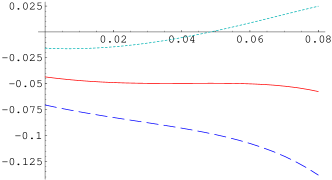
Figure 5: Free energy of the caloron gas in units of $T^{3}V$ at $T=1.3\Lambda$ (dotted), $T=1.125\Lambda$ (solid) and $T=1.05\Lambda$ (dashed) as function of the asymptotic value of $A_{4}$ in units of $2\pi T$.

Although several simplifying assumptions have been made in this derivation, it may indicate the instability of the trivial holonomy at temperatures below some critical one related to $\Lambda$.

Appendix A ADHM construction for the BPS dyon and the KvBLL caloron

A.1 General ADHM construction

The basic object in the ADHM construction  ADHM is the $k\times(k+1)$ quaternionic-valued matrix $\Delta$ which is taken to be linear in the space-time variable $x$:

$$\Delta(x)={\cal A}+{\cal B}x,\qquad x\equiv x_{\mu}\sigma_{\mu},\qquad\sigma_{\mu}=(i\vec{\tau},1_{2})\;.$$ (94)

The ADHM gauge potential is given by

$$A_{\mu}(x)=v^{\dagger}(x)\partial_{\mu}v(x),$$ (95)

where $v(x)$ is a $(k+1)$ dimensional quaternionic vector, the normalized solution to

$$\Delta^{\dagger}(x)v(x)=0,$$ (96)

and $k$ is the topological charge of the gauge field. An important property of the ADHM construction is that the operator $\Delta^{\dagger}(x)\Delta(x)$ is a real-valued matrix:

$$f=(\Delta(x)^{\dagger}\Delta(x))^{-1}\in{\rm I\kern-1.79993ptR}^{k\times k}\;.$$ (97)

In what follows we shall use the equation

$$\Delta f\Delta^{\dagger}=1-vv^{\dagger}\;.$$ (98)

It becomes obvious when one notes that both sides are projectors onto the space orthogonal to the vector $v$, which follows from $v^{\dagger}v=1$, $\Delta^{\dagger}v=0$.

In the case of finite temperatures, because of the infinite number of copies of space in the compact direction, the topological charge $k=\infty$, and it is convenient to make a discrete Fourier transformation with respect to the infinite range indices. The Fourier transformed $v(x)$ are $2\times 2$ matrix-valued functions $v(x_{\mu},z)$ of a new variable $z\in[-1/2,1/2]$ and $\Delta$ becomes a differential operator in $z$.

A.2 ADHM construction for the BPS dyon

As stated above, at nonzero temperatures the essence of the ADHM construction is the introduction of $2\times 2$ matrix-valued functions $v(x_{\mu},z)$. The scalar product is defined as

$$\langle v_{1}|v_{2}\rangle=\int^{1/2}_{-1/2}v^{+}_{1}(x_{\mu},z)v_{2}(x_{\mu},z)dz\;.$$ (99)

For the BPS dyon solution $v$ has been found by Nahm Nahm80 :

$$v(x_{\mu},z)=\sqrt{\frac{{\rm v}r}{\sinh({\rm v}r)}}\exp(iz{\rm v}x^{\dagger})$$ (100)

where $\sigma^{\dagger}_{\mu}=(1_{2},-i\vec{\tau}),\;x^{\dagger}=x_{\mu}\sigma^{\dagger}_{\mu}$ and $r=|\vec{x}|$). The matrix-valued function $v$ is the solution of the equation

$$\Delta^{\dagger}(x)v(x,z)=0,\;\;\;\;\;\Delta^{\dagger}(x)=i\partial_{z}+{\rm v}x^{\dagger}$$ (101)

normalized to unity,

$$\langle v|v\rangle=1.$$ (102)

The gauge field is expressed through $v$ as

$$A_{\mu}=\langle v|\partial_{\mu}v\rangle.$$ (103)

We use anti-hermitian fields such that the covariant derivative is $D_{\mu}=\partial_{\mu}+A_{\mu}$. Comparing eq.(101) with the general eq.(94) we conclude that in this case

$${\cal A}=-i\partial_{z},\;\;\;\;\;{\cal B}={\rm v}.$$ (104)

Eq.(100) corresponds to the ‘hedgehog’ gauge. However we find it more convenient to work in the ‘stringy’ gauge where $A_{\mu}$ has a pure gauge string-like singularity. One proceeds from the ‘hedgehog’ gauge to the ‘stringy’ gauge using the singular gauge transformation (see e.g. DPSUSY )

$$v\rightarrow v^{s}=vS_{-}^{\dagger},\quad A_{\mu}\rightarrow A_{\mu}^{s}=S_{-}A_{\mu}S_{-}^{\dagger}+S_{-}\partial_{\mu}S^{\dagger}_{-}$$ (105)

with

$$S_{-}=e^{-i\frac{\phi}{2}\tau^{3}}e^{i\frac{\pi-\theta}{2}\tau_{2}}e^{-i\frac{\phi}{2}\tau^{3}}$$ (106)

having the property that it “gauge-combs” $A_{4}$ at spatial infinity to a fixed (third) direction:

$$S_{-}n^{a}\tau^{a}S_{-}^{\dagger}=\tau^{3}\;.$$ (107)

In the ‘stringy’ gauge

$$v^{s}=S_{-}^{\dagger}\sqrt{\frac{{\rm v}r}{\sinh({\rm v}r)}}\exp[z{\rm v}(ix_{4}+r\tau^{3})]\;.$$ (108)

One can check that $A_{\mu}=\langle v^{s}|\partial_{\mu}v^{s}\rangle$ gives the M dyon field in the ‘stringy’ gauge as in eq.(13). We note that in the ‘stringy’ gauge $v^{s}$ has a remarkable property

$$v^{s}(x_{4}+n,\vec{x})=e^{in{\rm v}z}v^{s}(x_{4},\vec{x})\;.$$ (109)

A.3 ADHM construction for the KvBLL caloron

Unfortunately, the original paper KvB does not present an explicit expression for $v$, the main ingredient of the ADHM construction. We could have used ref. LL but it seems that ref. KvB is more informative in some other respects. Therefore, we have to calculate $v$ ourselves.

From the point of view of the original ADHM construction $v$ is a quaternionic vector of infinite length since finite-temperature field configuration can be viewed as an infinite set of equal strips, the total topological charge in ${\rm I\kern-1.79993ptR}^{4}$ being infinite. The bracket is formally defined as a contraction along this infinite-dimension side:

$$\langle v|\tilde{v}\rangle\equiv v^{\dagger}\tilde{v}\;.$$ (110)

The gauge potential results from

$$A_{\mu}(x)=v^{\dagger}(x)\partial_{\mu}v(x),\;\;\;\;\;D_{\mu}=\partial_{\mu}+A_{\mu}\;.$$ (111)

The vector $v(x)$ is the normalized solution of the equation

$$\Delta^{\dagger}(x)v(x)=0,\;\;\;\;\;\Delta(x)=\left(\!\!\begin{array}[]{c}\lambda\\ B-x\end{array}\!\!\right),$$ (112)

where $B$ is a square quaternionic matrix, $\lambda$ is an (infinite) quaternionic vector, $x\equiv x_{\mu}\sigma_{\mu},\;\sigma_{\mu}=(i\vec{\tau},1_{2})$. Introducing the notations

$$v(x)=\Phi^{-\frac{1}{2}}(x)\left(\!\!\begin{array}[]{c}-1\\ u(x)\end{array}\!\!\right),\quad u(x)=(B^{\dagger}-x^{\dagger})^{-1}\lambda^{\dagger}\;,$$ (113)

eq.(112) becomes

$$(B^{\dagger}-x^{\dagger})u(x)=\lambda^{\dagger}.$$ (114)

The inverse of the matrix $(B^{\dagger}-x^{\dagger})$ exists almost in all points. The points where it does not exists, are monopole positions. We are interested in those singular points that lie in the interval $0<x_{4}<1$ (we have rescaled the units to set temperature $T=1$). The unknown function $\Phi(x)$ is determined from the normalization of $v$:

$$\Phi(x)=1+u^{\dagger}u\;.$$ (115)

The formalism of infinite-dimensional matrices is not convenient. Following Nahm Nahm80 we pass to the Fourier transforms in the discrete but infinite-range indices and get instead a continuous variable $z\in[-\frac{1}{2},\frac{1}{2}]$. In the notations of ref. KvB :

$$(B^{\dagger}-x^{\dagger})_{nm}=-\int_{-1/2}^{1/2}\!\frac{dz}{2\pi i}\,e^{-2\pi izn}\hat{D}^{\dagger}_{x}(z)\,e^{2\pi izm},\qquad\hat{D}^{\dagger}_{x}(z)=-\partial_{z}+\hat{A}^{\dagger}(z)+2\pi ix^{\dagger}\equiv-\partial_{z}+2\pi ir^{\dagger}(z)\;,$$

where

$$\hat{A}(z)=2\pi i[\xi+{\overrightarrow{r_{12}}}\cdot\vec{\sigma}\Theta_{\omega}(z)].$$ (116)

Here the function $\Theta_{\omega}(z)=2\bar{\omega}$ when $z\in[-\omega,\omega]$ and $-2\omega$ otherwise; $r^{\dagger}(z)\equiv r_{\mu}(z)\sigma^{\dagger}_{\mu},\;x^{\dagger}\equiv x_{\mu}\sigma^{\dagger}_{\mu}$. As it can be seen from eq.(A.3), the quaternion $\xi$ simply represents the center of mass position of the whole system and can be set to zero, $\xi=0$. We define $r_{\mu}(z)=r_{\mu}$ when $z\in[\omega,1-\omega]$, and $r_{\mu}(z)=s_{\mu}$ otherwise, where

$$\vec{s}=\vec{x}-2\bar{\omega}{\overrightarrow{r_{12}}},\qquad\vec{r}=\vec{x}+2\omega{\overrightarrow{r_{12}}},\qquad s_{4}=r_{4}=x_{4}.$$ (117)

Here $\bar{\omega}\equiv\frac{1}{2}-\omega$, and $r_{\mu}$ and $s_{\mu}$ have the meaning of the vectors from the dyon centers to the ‘observation’ point, ${\overrightarrow{r_{12}}}=\vec{r}-\vec{s}$ has the meaning of dyon the separation. We choose dyons to be separated in the 3d direction: ${\overrightarrow{r_{12}}}=r_{12}\vec{e}_{3}$. As for $\lambda$,

$$\lambda_{n}^{\dagger}=\rho U^{\dagger}e^{-2\pi in\vec{\omega}\cdot\vec{\tau}},$$ (118)

where $U$ is a unitary matrix, and $\rho>0$. We have an additional constraint KvB

$${\overrightarrow{r_{12}}}\cdot\vec{\sigma}=\pi\rho^{2}(U^{\dagger}\vec{\omega}\cdot\vec{\sigma}U)/\omega\;.$$ (119)

Here $2\pi i\vec{\omega}\cdot\vec{\tau}$ is the value of $A_{4}$ at spatial infinity, $\omega=|\vec{\omega}|$. It can be seen that $\pi\rho^{2}=r_{12}$. We choose to rotate the $A_{4}$ direction in color space instead of rotating monopole positions, so we do not loose the generality of the solution. We connect the vector $\vec{\omega}$ and $U$ by

$$U^{\dagger}\vec{\omega}\cdot\vec{\tau}U=\omega\tau_{3}\;.$$ (120)

Writing down the $m^{\rm th}$ component of the (infinite) quaternionic vector as a Fourier transform

$$u_{m}(x)=\int_{-1/2}^{1/2}u(x,z)e^{-2\pi imz}dz,$$ (121)

eq.(112) we have to solve can be rewritten as

$$(\partial_{z}-2\pi ir^{\dagger}(z))u(x,z)=2\pi i\rho U^{\dagger}\sum_{n}e^{-2\pi in\vec{\omega}\cdot\vec{\tau}}e^{2\pi izn}=2\pi i\rho U^{\dagger}(P_{+}\delta(z-\omega)+P_{-}\delta(z+\omega)),$$ (122)

where

$$P_{\pm}=\frac{1}{2}(1\pm\vec{\omega}\cdot\vec{\tau}/\omega)\;.$$ (123)

Eq.(122) is piece-wise homogeneous, therefore we present its solution in the form

$$u(x,z)\!=\!\left\{\begin{array}[]{ll}\exp\!\left(2\pi is^{\dagger}z\right)\!B_{1},&-\omega\!<\!z\!<\!\omega\\ \exp\!\left(2\pi ir^{\dagger}(z\!-\!1/2)\right)\!B_{2},&\omega\!<\!z\!<\!1\!-\!\omega\end{array}\right.$$ (124)

and match the values and the derivatives of $u$ at the endpoints of the pieces,

$$e^{-2\pi ir^{\dagger}\bar{\omega}}B_{2}-e^{2\pi is^{\dagger}\omega}B_{1}=f_{1},\qquad e^{-2\pi is^{\dagger}\omega}B_{1}-e^{2\pi ir^{\dagger}\bar{\omega}}B_{2}=f_{2}\;,$$ (125)

where

$$f_{1}=2\pi i\rho U^{\dagger}P_{+},\qquad f_{2}=2\pi i\rho U^{\dagger}P_{-},\qquad\bar{\omega}=\frac{1}{2}-\omega.$$

Note that $B_{1,2}$ are matrices that generally do not commute:

$$B_{2}=\left(e^{-2\pi is^{\dagger}\omega}e^{-2\pi ir^{\dagger}\bar{\omega}}-e^{2\pi is^{\dagger}\omega}e^{2\pi ir^{\dagger}\bar{\omega}}\right)^{-1}\left(e^{-2\pi is^{\dagger}\omega}f_{1}+e^{2\pi is^{\dagger}\omega}f_{2}\right)\equiv b_{22}b_{21}e^{-2\pi ix_{4}\omega\tau_{3}}U^{\dagger}/\hat{\psi},$$ (126)

$$B_{1}=\left(e^{-2\pi ir^{\dagger}\bar{\omega}}e^{-2\pi is^{\dagger}\omega}-e^{2\pi ir^{\dagger}\bar{\omega}}e^{2\pi is^{\dagger}\omega}\right)^{-1}\left(e^{-2\pi ir^{\dagger}\bar{\omega}}f_{2}+e^{2\pi ir^{\dagger}\bar{\omega}}f_{1}\right)\equiv b_{12}b_{11}e^{-2\pi ix_{4}\omega\tau_{3}}U^{\dagger}/\hat{\psi},$$

where

$$b_{22} = \left[-\cos(\pi x_{4})({\rm ch_{\frac{1}{2}}}\,\overline{{\rm sh_{\frac{1}{2}}}}\,\hat{r}+\overline{{\rm ch_{\frac{1}{2}}}}\,{\rm sh_{\frac{1}{2}}}\,\hat{s})+i\sin(\pi x_{4})({\rm ch_{\frac{1}{2}}}\,\overline{{\rm ch_{\frac{1}{2}}}}+\hat{r}\,\hat{s}\,{\rm sh_{\frac{1}{2}}}\,\overline{{\rm sh_{\frac{1}{2}}}})\right],$$

$$b_{12} = \left[-\cos(\pi x_{4})({\rm ch_{\frac{1}{2}}}\,\overline{{\rm sh_{\frac{1}{2}}}}\,\hat{r}+\overline{{\rm ch_{\frac{1}{2}}}}\,{\rm sh_{\frac{1}{2}}}\,\hat{s})+i\sin(\pi x_{4})({\rm ch_{\frac{1}{2}}}\,\overline{{\rm ch_{\frac{1}{2}}}}+\hat{s}\,\hat{r}\,{\rm sh_{\frac{1}{2}}}\,\overline{{\rm sh_{\frac{1}{2}}}})\right],$$

$$b_{21} = 2\pi i\rho({\rm ch_{\frac{1}{2}}}-\hat{s}\,\tau_{3}\,{\rm sh_{\frac{1}{2}}}),\qquad b_{11}=2\pi i\rho(\overline{{\rm ch_{\frac{1}{2}}}}+\hat{r}\,\tau_{3}\,\overline{{\rm sh_{\frac{1}{2}}}})e^{\pi ix_{4}\tau_{3}},$$

$$\hat{\psi} \equiv -\cos(2\pi x_{4})+{\rm ch_{\frac{1}{2}}}\,\overline{{\rm ch_{\frac{1}{2}}}}+\frac{\vec{s}\cdot\vec{r}}{s\,r}{\rm sh_{\frac{1}{2}}}\,\overline{{\rm sh_{\frac{1}{2}}}}\,.$$ (127)

Hat over the variable (notation found also in KvB ) means contraction of the corresponding normalized vector with Pauli matrices, e.g. $\hat{\omega}\equiv\vec{\omega}\cdot\vec{\tau}/\omega$. We denote for brevity

$$\mathrm{sh}\,\equiv\sinh(4\pi s\omega),\qquad\mathrm{ch}\,\equiv\cosh(4\pi s\omega),\qquad\overline{\mathrm{sh}}\,\equiv\sinh(4\pi r\bar{\omega}),\qquad\overline{\mathrm{ch}}\,\equiv\cosh(4\pi r\omega),$$ (128)

and the hyperbolic functions with subscript “$\frac{1}{2}$” are the corresponding functions of half the same arguments. Combining eqs.(124,126,127) back into eq.(113) one gets the two-dimensional quaternionic vector $v(x,z)$ which is the base for the construction of the Green’s function, see Appendix B. Note that we have made a Fourier transform of $u$ (121) and got a continuous index $z$, so that scalar products of infinite-dimensional vectors become $z$ integrations, see eq.(131).

We note that $U$ is actually a gauge transformation of $v$. Therefore, the gauge potential $A_{\mu}^{U}$ is obtained by a global gauge transformation of $A_{\mu}^{U=1}$. We conclude that the determinant does not depend on the relative ‘color orientation’ of the Polyakov line or holonomy, and of the vector $\overrightarrow{r_{12}}$ connecting monopole centers. Thus, we set $U=1$ and $\vec{\omega}=\omega\vec{e}_{3}$.

We notice further that $v(x,z)$ built above gives $A_{\mu}$ that is not periodic in time direction and zero $A_{4}$ at spatial infinity. It is a peculiar feature of the ‘algebraic’ gauge used in KvB . It is more convenient to use the gauge in which the fields are periodic. To that end we make a non-periodic gauge transformation $g=e^{2\pi ix_{4}\omega\tau_{3}}$ and obtain

$$v(x,z)^{\rm per}=\Phi^{-\frac{1}{2}}(x)\left(\!\!\begin{array}[]{c}-g\\ w(x,z)\end{array}\!\!\right),\;\;\;w\!=\!ug,$$ (129)

meaning

$$w(x,z)=u(x,z)\;e^{2\pi ix_{4}\omega\tau_{3}}.$$ (130)

In terms of the Fourier-transformed $v$ the bracket takes the form

$$\langle v|\tilde{v}\rangle\equiv v_{1}^{\dagger}\tilde{v}_{1}+\int_{-1/2}^{1/2}v_{2}^{\dagger}\tilde{v}_{2}\;dz\,,$$ (131)

where $v_{1}$ is an upper element and $v_{2}$ is a lower one.

Now let us determine $\Phi(x)$. We use the following identities:

$$b_{12}^{\dagger}b_{12}=b_{22}^{\dagger}b_{22}=\hat{\psi}/2,\qquad b_{21}^{\dagger}b_{21}=4\pi^{2}\rho^{2}\left({\rm ch_{\frac{1}{2}}}-\frac{s_{3}}{s}\,{\rm sh_{\frac{1}{2}}}\right),\qquad b_{11}^{\dagger}b_{11}=4\pi^{2}\rho^{2}\left(\overline{{\rm ch_{\frac{1}{2}}}}+\frac{r_{3}}{r}\,\overline{{\rm sh_{\frac{1}{2}}}}\right).$$ (132)

Note that the right-hand sides of eq.(132) are proportional to the unity $2\times 2$ matrix. Now we can easily calculate the normalization:

$$\langle v|v\rangle = {\hat{\psi}}^{-2}b_{11}^{\dagger}b_{11}b_{12}^{\dagger}b_{12}\int_{-\omega}^{\omega}\!dz\,e^{-4\pi\vec{s}\cdot\vec{\tau}z}+{\hat{\psi}}^{-2}b_{21}^{\dagger}b_{21}b_{22}^{\dagger}b_{22}\int_{-\bar{\omega}}^{\bar{\omega}}\!dz\,e^{-4\pi\vec{r}\cdot\vec{\tau}z}$$

$$= \frac{\pi\rho^{2}}{\hat{\psi}}\left[\left(\frac{\overline{{\rm ch_{\frac{1}{2}}}}\,{\rm sh_{\frac{1}{2}}}}{s}+\frac{{\rm ch_{\frac{1}{2}}}\,\overline{{\rm sh_{\frac{1}{2}}}}}{r}\right)+\frac{r_{12}}{s\,r}{\rm sh_{\frac{1}{2}}}\,\overline{{\rm sh_{\frac{1}{2}}}}\right]\equiv\frac{\psi-\hat{\psi}}{\hat{\psi}}\;.$$

We used the identity $\vec{r}-\vec{s}=\overrightarrow{r_{12}}=r_{12}\vec{e}_{3}$. Thus for $\Phi$ we get

$$\Phi=\frac{\psi}{\hat{\psi}},\qquad\psi=\hat{\psi}+r_{12}\left(\frac{\overline{{\rm ch_{\frac{1}{2}}}}\,{\rm sh_{\frac{1}{2}}}}{s}+\frac{{\rm ch_{\frac{1}{2}}}\,\overline{{\rm sh_{\frac{1}{2}}}}}{r}\right)+\frac{r_{12}^{2}}{s\,r}{\rm sh_{\frac{1}{2}}}\,\overline{{\rm sh_{\frac{1}{2}}}}\;.$$ (133)

We have checked the $A_{\mu}$ of the KvBLL caloron (7) by calculating $\langle v^{\rm per}|\partial_{\mu}v^{\rm per}\rangle$. Note that $v^{\rm per}$ has the following periodicity property (only for integer $n$):

$$v^{\rm per}(z,x_{4}+n)=e^{2\pi inz}v^{\rm per}(z,x_{4})\;.$$ (134)

Appendix B Spin-0 isospin-1 propagator

B.1 General construction of the Green function

Once the self-dual field is found in terms of the ADHM construction, such that the gauge field is written as $A_{\mu}=\langle v|\partial_{\mu}v\rangle$ where the scalar product is defined in eq.(131), it is possible to construct explicitly the Green function of spin-0 isospin-1 field in the background of the self-dual field Nahm80 ; KvB ; LL . The solution of the equation

$$-\left(D_{\mu}^{2}\right)^{ca}(x)G^{ab}(x,y)=\delta^{cb}\,\delta^{(4)}(x-y)$$ (135)

is given by

$$G^{ab}(x,y) = \frac{\frac{1}{2}{\rm Tr}\,\tau^{a}\langle v(x)|v(y)\rangle\tau^{b}\langle v(y)|v(x)\rangle}{4\pi^{2}(x-y)^{2}}$$ (136)

$$+ \frac{1}{4\pi^{2}}\int_{-1/2}^{1/2}dz_{1}\,dz_{2}\,dz_{3}\,dz_{4}\,M(z_{1},z_{2},z_{3},z_{4})\frac{1}{2}{\rm Tr}\!\left({\cal V}^{\dagger}(x,z_{1}){\cal V}(x,z_{2})\tau^{a}\right){\rm Tr}\!\left({\cal V}^{\dagger}(y,z_{4}){\cal V}(y,z_{3})\tau^{b}\right)\,,$$

where ${\cal V}(x,z)\equiv{\cal B}^{\dagger}v(x,z)$.

We denote the first term by $G_{1}$ and the second term (the M-part) by $G_{2}$. The only new object is the function $M(z_{1},z_{2},z_{3},z_{4})$ which we determine bellow. As we shall see, we do not need $M$ with arbitrary arguments, but only at $z_{3}=z_{4}$. For coincident arguments we obtain

$$M(z_{1},z_{2},z,z)=\delta(z_{1}-z_{2})M(z_{1},z),$$ (137)

see below.

The propagator (136) is written for the ${\rm I\kern-1.79993ptR}^{4}$ space and does not obey the periodicity condition. The periodic propagator, however, can be easily obtained from it by a standard procedure:

$${\cal G}(x,y)=\sum_{n=-\infty}^{+\infty}G(x_{4},{\vec{x}};y_{4}+n,{\vec{y}}).$$ (138)

In what follows it will be convenient to split it into three parts:

$${\cal G}(x,y)={\cal G}^{\rm r}(x,y)+{\cal G}^{\rm s}(x,y)+{\cal G}^{\rm m}(x,y),$$

$${\cal G}^{\rm s}\equiv\left.G_{1}\right|_{n=0},\qquad{\cal G}^{\rm r}\equiv\sum\limits_{n\neq 0}G_{1},\qquad{\cal G}^{\rm m}\equiv\sum_{n}G_{2}\;.$$ (139)

The vacuum current (20) will be also split into three parts, in accordance to which part of the periodic propagator (139) is used to calculate it:

$$J_{\mu}=J^{\rm r}_{\mu}+J^{\rm s}_{\mu}+J^{\rm m}_{\mu}\;.$$ (140)

B.2 Propagator in the BPS dyon background

In Appendix A.2 we have found the needed periodic quaternion $v(x,z)$ for the single BPS monopole (see eq.(108)). The 4-argument function $M$ for the BPS monopole was computed in ref. Nahm80 . The result with the two last arguments taken equal is

$$M(z_{3},z_{4},z,z)=\delta(z_{3}-z_{4})M(z_{3},z),$$

$$M(z,z^{\prime})=-\frac{1}{4{\rm v}^{2}}\left(2|z-z^{\prime}|-1+4zz^{\prime}\right)\;.$$ (141)

Eqs.(108,141) completely determine the periodic propagator defined in eqs.(136,138) in the BPS dyon background. The use of this propagator is demonstrated in Appendix C.

B.3 Propagator in the KvBLL caloron background

In Appendix A.3 we have found the needed quaternion $v(x,z)$ for the KvBLL caloron. In this Appendix we derive the $M$-function for the KvBLL caloron. The propagator (136) will be then completely determined in the caloron background.

In the notations of Nahm80 $M$ is an infinite-dimensional rank-4 tensor, with indices running from 1 to $k$, the topological charge in ${\rm I\kern-1.79993ptR}^{4}$. As in the case of $v$, it is convenient to make the Fourier transformation with respect to the indices:

$$M_{pqnm}=\int_{-1/2}^{1/2}M(z_{1},z_{2},z_{3},z_{4})\,e^{2\pi i(\!-\!pz_{1}\!+\!qz_{2}\!+\!nz_{3}\!-\!mz_{4})}dz_{1}dz_{2}dz_{3}dz_{4}.$$ (142)

The tensor $M_{pqmn}$ is defined by the equation CWS

$$\frac{1}{2}{\rm Tr}[({\cal A}^{\dagger}{\cal A})_{il}({\cal B}^{\dagger}{\cal B})_{mj}+({\cal B}^{\dagger}{\cal B})_{il}({\cal A}^{\dagger}{\cal A})_{mj}-2({\cal A}^{\dagger}{\cal B})_{il}({\cal B}^{\dagger}{\cal A})_{mj}]M_{rsij}=\delta_{rl}\delta_{sm}\;,$$ (143)

All indices here run from 1 to $k$ as rectangular $k\times(k+1)$ matrices ${\cal A}$ and ${\cal B}$ are contracted along the longer side. Here ${\cal A}$ and ${\cal B}$ are:

$$\Delta(x)\equiv{\cal A}+{\cal B}x,\quad{\cal A}=\Delta(0),\quad{\cal B}=\left(\!\!\begin{array}[]{c}0\\ -1\end{array}\!\!\right)\;.$$ (144)

Eq.(143) can be rewritten as

$$\frac{1}{2}{\rm Tr}[(\Delta^{\dagger}\Delta(0))_{il}\delta_{mj}+(\Delta^{\dagger}\Delta(0))_{mj}\delta_{il}-2B^{\dagger}_{il}B_{mj}]M_{rsij}=\delta_{rl}\delta_{sm}\;,$$ (145)

where $\Delta^{\dagger}\Delta(0)=\lambda^{\dagger}\lambda+B^{\dagger}B$, $\;B$ and $\lambda$ are found in eq.(A.3) and eq.(118), respectively. In our case $k$ is infinite and we rewrite eq.(145) in the Fourier basis:

$$\frac{1}{2}{\rm Tr}\left[\tilde{\Delta}^{\dagger}\tilde{\Delta}(0,z_{3})+\tilde{\Delta}^{\dagger}\tilde{\Delta}(0,z_{4})+2\left(\frac{\partial_{z_{3}}}{2\pi i}+r^{\dagger}(z_{3})\right)\left(\frac{\partial_{z_{4}}}{2\pi i}-r(z_{4})\right)\right]M(z_{1},z_{2},z_{3},z_{4})=\delta(z_{1}-z_{3})\delta(z_{2}-z_{4})\;,$$

where $r(z)=r_{i}\sigma_{i}$ when $z\in[\omega,1-\omega]$, and $r(z)=s_{i}\sigma_{i}$ otherwise; $\sigma_{i}=i\tau_{i}$. Zero components of $r_{\mu},\;s_{\mu}$ are absent because $x_{\mu}=0$. We use

$$\tilde{\Delta}^{\dagger}\tilde{\Delta}(0,z)=\!-\!\frac{\partial_{z}^{2}}{4\pi^{2}}\!+\!r^{2}(z)\!+\!\frac{\rho^{2}}{2}\left(\delta(z\!-\!\omega)\!+\!\delta(z\!+\!\omega)\right)\;.$$ (146)

Here the first two terms come from the Fourier transformation of $B^{\dagger}B$ (A.3) and the last one comes from the Fourier transformation of $\lambda^{\dagger}\lambda$. We obtain the explicit equation for $M$:

$$\left(-\frac{(\partial_{z_{3}}+\partial_{z_{4}})^{2}}{4\pi^{2}}+|\vec{r}(z_{3})-\vec{r}(z_{4})|^{2}\right)M(z_{1},z_{2},z_{3},z_{4})+$$

$$+\frac{\rho^{2}}{2}\left(\delta(\!z_{3}\!-\!\omega\!)+\delta(\!z_{3}\!+\!\omega\!)+\delta(\!z_{4}\!-\!\omega\!)+\delta(\!z_{4}\!+\!\omega\!)\right)M(z_{1},z_{2},z_{3},z_{4})=\delta(z_{1}-z_{3})\delta(z_{2}-z_{4})\;.$$ (147)

In the case $z_{3}=z_{4}$, which is the only one we need as we shall see in a moment, we look for the solution in the form

$$M(z_{1},z_{2},z,z)=\delta(z_{1}-z_{2})M(z_{1},z)\;.$$ (148)

The equation for the two-argument function simplifies to

$$\left(-\frac{\partial_{z}^{2}}{4\pi^{2}}+\frac{r_{12}}{\pi}\delta(z-\omega)+\frac{r_{12}}{\pi}\delta(z+\omega)\right)M(z^{\prime},z)=\delta(z-z^{\prime})\;,$$ (149)

where $r_{12}=\pi\rho^{2}$. We see that the solution has to be piece-wise linear in its arguments. The solution is symmetric in its two arguments and for $z<z^{\prime}$ is given by

$$M(z,z^{\prime})=\left\{\begin{array}[]{ll}\frac{32r_{12}^{2}{\pi^{3}}\omega(z-\omega)(1-z^{\prime}-\omega)-8r_{12}\pi^{2}({{\omega}^{2}}+z(z^{\prime}-1))+\pi}{2d(8r_{12}\pi\omega\bar{\omega}+1)},\quad z,z^{\prime}\in[\omega,1-\omega]\\ \frac{1}{2}\pi\left(\frac{4\pi z(1-2z^{\prime})}{8r_{12}\pi\omega\bar{\omega}+1}+\frac{1}{r_{12}}\right),\quad\quad\quad\quad\quad\quad\quad\quad\quad z\in[-\omega,\omega],z^{\prime}\in[\omega,1-\omega]\\ \frac{4r_{12}\pi^{2}[z-z^{\prime}-2z^{\prime}z-2(\omega-1)\omega-8r_{12}\pi(z^{\prime}-\omega)(z+\omega)\bar{\omega}]+\pi}{2r_{12}(8r_{12}\pi\omega\bar{\omega}+1)},\quad z,z^{\prime}\in[-\omega,\omega]\end{array}\right.\;.$$ (153)

Outside this range $M$ is defined by periodicity: $M(z+n,z^{\prime}+m)=M(z,z^{\prime})$, where $n,m$ are integers.

Now let us demonstrate that actually only the two-argument function $M(z,z^{\prime})$ is needed to construct the propagator satisfying the periodicity. It turns out that making the Green function periodic simplifies $G_{2}$ (section III). One has from the definitions (136)-(139):

$${\cal G}^{\rm m}\equiv\sum_{n}\frac{1}{8\pi^{2}}\int_{-1/2}^{1/2}\!dz_{1}\!\dots\!dz_{4}\,M(\!z_{1}\!\dots\!z_{4}\!)\,{\rm Tr}\!\left(\!{\cal V}^{\dagger}(x,z_{1}){\cal V}(x,z_{2})\tau^{a}\!\right){\rm Tr}\!\left(\!{\cal V}^{\dagger}(y^{n},z_{4}){\cal V}(y^{n},z_{3})\tau^{b}\!\right)\;,$$ (154)

where $y^{n}_{4}=y_{4}+n,\;\vec{y}^{n}=\vec{y}$. Using eq.(134) we put

$${\cal V}(y^{n},z)=e^{2\pi i\eta nz}{\cal V}(y,z)$$ (155)

Further on, we note that for $|\eta|\leq 1$ one has

$$\sum_{n}{\rm Tr}\!\left({\cal V}^{\dagger}(y^{n},z_{4}){\cal V}(y^{n},z_{3})\tau^{b}\right)={\rm Tr}\!\left({\cal V}^{\dagger}(y,z_{4}){\cal V}(y,z_{3})\tau^{b}\right)\delta(z_{3}-z_{4})\frac{1}{|\eta|}\;.$$

Now we can see that making the Green’s function periodic results in the substitution

$$M(z_{1},z_{2},z_{3},z_{4})\rightarrow\frac{1}{|\eta|}M(z_{1},z_{2},z_{3},z_{3})\delta(z_{3}-z_{4})=\frac{1}{|\eta|}M(z_{1},z_{3})\delta(z_{1}-z_{2})\delta(z_{3}-z_{4})\;.$$

It follows from eq.(109) and eq.(134) that for the monopole one has to take $\eta={\rm v}/(2\pi)<1$ and for the KvBLL caloron $\eta=1$. In both cases the $M$-part of the periodic propagator is given by

$${\cal G}^{\rm m}=\frac{1}{8\pi^{2}|\eta|}\int_{-1/2}^{1/2}dzdz^{\prime}M(z,z^{\prime})\,{\rm Tr}\left({\cal V}^{\dagger}(x,z){\cal V}(x,z)\tau^{a}\right)\,{\rm Tr}\left({\cal V}^{\dagger}(y,z^{\prime}){\cal V}(y,z^{\prime})\tau^{b}\right),$$ (156)

where the two-argument $M$ functions are found in eq.(141) and eq.(153), respectively.

Appendix C Vacuum current in the BPS monopole background

We compute the vacuum current (20) in the BPS monopole background in this Appendix. We assume $0<{\rm v}<2\pi$ and work in the stringy gauge (13) dropping the index $s$ in $v^{s}$ given by eq.(108).

C.1 Singular part of the monopole current $J^{\rm s}_{\mu}$

This part of the current corresponds to the second term ${\cal G}^{\rm s}$ in eq.(139). At $x\rightarrow y$ this part of the propagator is singular. The regularization is presented in Appendix E. Eqs.(E,104) state:

$${J^{\rm s}_{\mu}}^{ab}=i\varepsilon^{adb}{\rm tr}\left(\tau^{d}j_{\mu}\right),\qquad j_{\mu}=\frac{{\rm v}^{2}}{12\pi^{2}}\left\langle v\left|f\sigma_{\mu}\Delta^{\dagger}f\right|v\right\rangle-{\rm h.c.},\qquad\Delta^{\dagger}(x)=i\partial_{z}+{\rm v}x^{\dagger}\;.$$ (157)

The function $f(z,z^{\prime},x)$ for the BPS monopole is known Nahm80 :

$$f(x;z,z^{\prime})=-\frac{e^{i{\rm v}x_{4}(z-z^{\prime})}}{2{\rm v}s}\left(\sinh{\rm v}s|z-z^{\prime}|+\coth\frac{{\rm v}s}{2}\,\sinh{\rm v}sz\,\sinh{\rm v}sz^{\prime}-\tanh\frac{{\rm v}s}{2}\,\cosh{\rm v}sz\,\cosh{\rm v}sz^{\prime}\right).$$ (158)

Here we denoted by $s$ the distance to the M-monopole center. It is helpful to calculate the action of the Green function on $v$. Since monopole is a static configuration, we can take $x_{4}=0$, moreover $f$ is a scalar function and we can move $S^{\dagger}_{-}$ matrix to the left:

$$\left.|\nu{\rangle}\equiv S_{-}f|v{\rangle}\right|_{x_{4}=0}=\frac{\cosh(svz)\tanh(sv/2)-2z\sinh(svz)}{4\sqrt{sv\sinh(sv)}}1_{2}+\frac{\sinh(svz)\coth(sv/2)-2z\cosh(svz)}{4\sqrt{sv\sinh(sv)}}\tau_{3}\;.$$

We use the following identities

$$S_{-}\vec{n}_{r}\vec{\tau}S_{-}^{\dagger}=\tau_{3}\;,$$

$$S_{-}\vec{n}_{\theta}\vec{\tau}S_{-}^{\dagger}=-\cos(\phi)\tau_{1}-\sin(\phi)\tau_{2}\;,$$

$$S_{-}\vec{n}_{\phi}\vec{\tau}S_{-}^{\dagger}=\sin(\phi)\tau_{1}-\cos(\phi)\tau_{2}$$ (159)

and arrive, after simple algebra, to

$$\{j_{4},j_{r},j_{\theta},j_{\phi}\}=\frac{{\rm v}^{3}}{12\pi^{2}}{\langle}\nu|\{i,-\tau_{3},\cos\!\phi\;\tau_{1}\!+\!\sin\!\phi\;\tau_{2},-\!\sin\!\phi\;\tau_{1}\!+\!\cos\!\phi\;\tau_{2}\}(\partial_{z}-{\rm v}\tau_{3}s)|\nu{\rangle}+{\rm h.c.}\;.$$

Finally we obtain the singular part of the vacuum current:

$$J^{\rm s}_{r} = 0,$$

$$J^{\rm s}_{\phi} = -\frac{i{\rm v}\left(s^{2}{\rm v}^{2}{\mathrm{csch}^{2}(s{\rm v})+s{\rm v}\coth(s{\rm v})-2}\right)}{24\pi^{2}s^{2}\sinh(s{\rm v})}(T_{1}\cos(\phi)+T_{2}\sin(\phi)),$$

$$J^{\rm s}_{\theta} = -\frac{i{\rm v}\left(s^{2}{\rm v}^{2}{\mathrm{csch}^{2}(s{\rm v})+s{\rm v}\coth(s{\rm v})-2}\right)}{24\pi^{2}s^{2}\sinh(s{\rm v})}(T_{1}\sin(\phi)-T_{2}\cos(\phi)),$$

$$J^{\rm s}_{4} = -\frac{i\left(1-s^{3}{\rm v}^{3}\coth(s{\rm v}){\mathrm{csch}^{2}(s{\rm v})}\right)}{24\pi^{2}s^{3}}T_{3}\;,$$ (160)

where ${(T_{c})}^{ab}\equiv i\varepsilon^{acb}$.

C.2 Regular part of the monopole current $J^{\rm r}_{\mu}$

We are going to calculate the part of the current that corresponds to

$$({\cal G}^{{\rm r}})^{ab}(x,y)\equiv\sum_{n\neq 0}\frac{1}{8\pi^{2}(x-y_{n})^{2}}{\rm Tr}\left[\tau^{a}{\langle}v(x)|v(y_{n}){\rangle}\tau^{b}{\langle}v(y_{n})|v(x){\rangle}\right],\qquad y_{n}=\vec{y},\quad y_{n4}=y_{4}+n,$$ (161)

namely

$$J^{\rm r}_{\mu}=J^{{\rm r}1}_{\mu}+J^{{\rm r}2}_{\mu},\qquad J^{{\rm r}1}_{\mu}=A_{\mu}{\cal G}^{{\rm r}}+{\cal G}^{{\rm r}}A_{\mu},\qquad J^{{\rm r}2}_{\mu}=(\partial^{x}_{\mu}-\partial^{y}_{\mu}){\cal G}^{{\rm r}}\;.$$

At first consider $J^{{\rm r}1}_{\mu}$. We have to compute ${\cal G}^{{\rm r}}$ with equal arguments. Substituting (108) into (161) and calculating the trace one has

$$({\cal G}^{{\rm r}})^{ab}(x,x)\equiv\sum_{n\neq 0}\int dzdz^{\prime}\frac{{\rm Tr}}{8\pi^{2}n^{2}},$$ (162)

where

$${\rm Tr}=2\frac{s^{2}{\rm v}^{2}e^{in{\rm v}(z-z^{\prime})}}{\sinh^{2}(s{\rm v})}\left[\cosh(2s{\rm v}(z-z^{\prime}))(\delta^{ab}-\delta^{a3}\delta^{b3})+\cosh(2s{\rm v}(z\!+\!z^{\prime}))\delta^{a}_{3}\delta^{b}_{3}\!+\!\sinh(2s{\rm v}(z\!-\!z^{\prime}))T_{3}^{ab}\right]$$

with $T^{c}=i\varepsilon^{acb}$. To compute the sum in this expression we use the summation formula (note that ${\rm v}<2\pi$)

$$\sum_{n\neq 0}\frac{e^{izn}}{4\pi^{2}n^{2}}=\frac{z^{2}}{8\pi^{2}}-\frac{|z|}{4\pi}+\frac{1}{12},\qquad-2\pi<z<2\pi\;.$$ (163)

It remains now to calculate integrals over $z$ and $z^{\prime}$. The result is

$${{\cal G}^{\rm r}}(x,x) = \left[\frac{3\coth(s{\rm v})-s{\rm v}(3\mathrm{csch}^{2}(s{\rm v})+2)}{8\pi s}+\frac{(s{\rm v}\coth(s{\rm v})-1)^{2}}{8\pi^{2}s^{2}}\right](\delta^{ab}-\delta^{a}_{3}\delta^{b}_{3})$$

$$+ \left[\frac{s{\rm v}\;\mathrm{csch}^{2}(s{\rm v})-\coth(s{\rm v})}{8\pi s}+\frac{1-s^{2}{\rm v}^{2}\;\mathrm{csch}^{2}(s{\rm v})}{16\pi^{2}s^{2}}+\frac{1}{12}\right]\delta^{ab}\;.$$

Now we turn to the $J^{{\rm r}2}_{\mu}$ part of the current where we have to sum over $n$ a derivative of the propagator. First of all we consider derivatives of the trace in (161). One finds for $x=y$:

$$(\partial^{x}_{\theta}-\partial^{y}_{\theta}){\rm Tr} \!\!\!= \!\!\!\frac{2s^{2}{\rm v}^{2}i}{\sinh(s{\rm v})^{2}}(\cosh(2s{\rm v}z)+\cosh(2s{\rm v}z^{\prime}))(T_{1}\sin\phi-T_{2}\cos\phi)e^{i{\rm v}n(z-z^{\prime})}\,,$$

$$(\partial^{x}_{\phi}-\partial^{y}_{\phi}){\rm Tr} \!\!\!= \!\!\!\left(\sin\theta\frac{4s^{2}{\rm v}^{2}i}{\sinh(s{\rm v})^{2}}\cosh(s{\rm v}(z+z^{\prime}))\cosh(s{\rm v}(z-z^{\prime}))(T_{1}\cos\phi+T_{2}\sin\phi)\right.$$

$$\!\!\!\left.-\frac{4s^{2}{\rm v}^{2}i}{\sinh(s{\rm v})^{2}}\cosh(2s{\rm v}(z-z^{\prime}))(1-\cos\theta)T_{3}\right)e^{i{\rm v}n(z-z^{\prime})}\,,$$

$$(\partial^{x}_{4}-\partial^{y}_{4}){\rm Tr} \!\!\!= \!\!\!-\frac{4s^{2}{\rm v}^{3}i}{\sinh^{2}(s{\rm v})}(z-z^{\prime})\sinh(2s{\rm v}(z-z^{\prime}))T_{3}e^{i{\rm v}n(z-z^{\prime})}\,,$$

$$(\partial^{x}_{s}-\partial^{y}_{s}){\rm Tr} \!\!\!= \!\!\!0\;.$$ (164)

Here only terms even in $z-z^{\prime}$ were left. The last two equations are especially clear as we can drop out the matrices $S$ in eq.(108).

A derivative of the denominator of (161) is equal to zero for $x=y$ except for the derivative with respect to $x_{4}$, but in this case we have the expression of the form (162) with $n^{3}/4$ instead of $n^{2}$ in the denominator. Now we can sum over $n$. We use the summation formula

$$\sum_{n\neq 0}\frac{e^{izn}}{i\pi^{2}n^{3}}=\frac{z^{3}}{6\pi^{2}}-\frac{z|z|}{2\pi}+\frac{z}{3},\;\;\;\;\;-2\pi<z<2\pi\;.$$ (165)

Next one has to integrate over $z,\;z^{\prime}$. Combining all pieces we obtain:

$$J^{\rm r}_{r} = 0,$$

$$J^{\rm r}_{\phi} = i\frac{\cos(\phi)T_{1}+\sin(\phi)T_{2}}{48\sinh^{3}(s{\rm v})\pi^{2}s^{2}}\wp_{1},$$

$$J^{\rm r}_{\theta} = i\frac{\sin(\phi)T_{1}-\cos(\phi)T_{2}}{48\sinh^{3}(s{\rm v})\pi^{2}s^{2}}\wp_{1},$$

$$J^{\rm r}_{4} = \frac{iT_{3}}{24{\pi}^{2}s^{3}}\wp_{2},$$ (166)

where we denote

$$\wp_{1} \equiv (s^{2}{\rm v}^{3}+6\pi s^{2}{\rm v}^{2}+3{\rm v}+3s({\rm v}+\pi)\sinh(2s{\rm v}){\rm v}-(s^{2}{\rm v}^{3}+3{\rm v}+6\pi)\cosh(2s{\rm v})+6\pi),$$

$$\wp_{2} \equiv 8{\pi}^{2}s^{2}(-1+s{\rm v}\coth(s{\rm v}))-12\pi s\coth(s{\rm v}){(-1+s{\rm v}\coth(s{\rm v}))}^{2}$$

$$+ (-3(1+4s^{2}{\rm v}^{2})+s{\rm v}(4(3+s^{2}{\rm v}^{2})\coth(s{\rm v})+3s{\rm v}(-4+s{\rm v}\coth(s{\rm v})){\mathrm{csch}^{2}(s{\rm v})})).$$

We have used spherical coordinates. For example, a projection of $\vec{J}$ onto the direction $\vec{n}_{\theta}=(\cos\theta\cos\phi,\cos\theta\sin\phi,-\sin\theta)$ is denoted by $J_{\theta}$.

C.3 M-part of the monopole current $J^{\rm m}_{\mu}$

Combining together eqs.(141,156) we have for the $M$-part of the periodic Green’s function:

$${\cal G}^{\rm m}=-\frac{{\rm v}}{16\pi}\int_{-1/2}^{1/2}\!dzdz^{\prime}\!\left(2|z\!-\!z^{\prime}|\!-\!1\!+\!4zz^{\prime}\right)\,{\rm Tr}\!\left(\!v^{\dagger}(x,z)v(x,z)\tau^{a}\!\right)\,{\rm Tr}\!\left(\!v^{\dagger}(y,z^{\prime})v(y,z^{\prime})\tau^{b}\!\right)$$ (167)

Note that we can drop out $S_{-}$ in (108). In the stringy gauge one has

$${v}^{\dagger}(x_{\mu},z)v(x_{\mu},z)=\frac{{\rm v}s}{\sinh({\rm v}s)}\exp[-2{\rm v}s\tau^{3}z]\;.$$ (168)

It means that ${\cal G}^{\rm m}$ has only the ‘33’ component. Taking the trace we get:

$${\rm Tr}\left[{v}^{\dagger}(x_{\mu},z)v(x_{\mu},z)\tau^{3}\right]=-2\frac{{\rm v}s}{\sinh({\rm v}s)}\sinh(2{\rm v}sz)\;.$$ (169)

Therefore the only nonzero component of ${\cal G}^{\rm m}$ is

$${\cal G}^{33}_{\rm m}(x,y)=-\frac{{\rm v}^{3}r_{x}r_{y}}{4\pi}\int_{-1/2}^{1/2}\!dzdz^{\prime}\left(2|z\!-\!z^{\prime}|\!-\!1\!+\!4zz^{\prime}\right)\,\frac{\sinh(2{\rm v}r_{y}z^{\prime})\sinh(2{\rm v}r_{x}z)}{\sinh({\rm v}r_{x})\sinh({\rm v}r_{y})}\;,$$

($r_{x}=|\vec{x}|$, $r_{y}=|\vec{y}|$). Performing the integrations we get

$${\cal G}^{33}_{\rm m}(x,y)=-\frac{1}{4\pi{\rm v}}\left(\frac{1}{r_{x}r_{y}}+\frac{{\rm v}r_{x}\coth{\rm v}r_{y}-{\rm v}r_{y}\coth{\rm v}r_{x}}{r^{2}_{y}-r^{2}_{x}}\right)\,.$$ (170)

Note that (170) is symmetric in its arguments. For that reason the contribution to the current coming from (ordinary) derivatives of ${\cal G}^{\rm m}$ is zero,

$$\left.\partial_{x}{\cal G}^{\rm m}(x,y)-\partial_{y}{\cal G}^{\rm m}(x,y)\right|_{x=y}=0,$$

and only the anticommutator $\{{\cal G}^{\rm m}(x,x),A_{\mu}\}$ remains. Taking the limit $x\rightarrow y$ we get for ${\cal G}^{\rm m}$

$${\cal G}^{33}_{\rm m}(x,x)=\frac{1}{8\pi s}\left[\coth({\rm v}s)-\frac{2}{{\rm v}s}+\frac{{\rm v}s}{\sinh^{2}({\rm v}s)}\right]$$ (171)

and for the contribution to the current $J^{\rm m}_{\mu}=A_{\mu}{\cal G}^{\rm m}+{\cal G}^{\rm m}A_{\mu}$ we obtain in spherical coordinates

$$J^{\rm m}_{r}=0,$$

$$J^{\rm m}_{\phi}=-\frac{i(\sin(\phi)T_{2}+\cos(\phi)T_{1})\left(s{\rm v}\coth(s{\rm v})+{s}^{2}{\rm v}^{2}{\mathrm{csch}^{2}(s{\rm v})}-2\right)}{16\pi\sinh(s{\rm v})s^{2}},$$

$$J^{\rm m}_{\theta}=-\frac{i(\sin(\phi)T_{1}-\cos(\phi)T_{2})\left(s{\rm v}\coth(s{\rm v})+{s}^{2}{\rm v}^{2}{\mathrm{csch}^{2}(s{\rm v})}-2\right)}{16\pi\sinh(s{\rm v})s^{2}},$$

$$J^{\rm m}_{4}=0\;.$$ (172)

Adding up (160,166) and (172) we obtain the full vacuum current in the BPS background, see eq.(IV.1) of the main text.

Appendix D Vacuum current in the KvBLL caloron background

There are no principal problems to make the calculation of the caloron Green’s function and the ensuing vacuum currents exactly. One can consider this Appendix as an instruction how to perform the exact calculation. In fact, we have done it but unfortunately the exact result for the current is about 200 pages long and thus too large to be printed. However, in certain limits the expressions drastically simplify. In particular, assuming the case when the dyons inside the caloron are widely separated such that their cores do not overlap, it is relatively easy to find the KvBLL caloron current with the exponential precision (i.e. dropping out term of the order $e^{-r\overline{{\rm v}}},\;e^{-s{\rm v}}$). This will be sufficient to find the determinant of the KvBLL caloron for large $r_{12}$ up to some constant.

With the exponential precision, the only nonzero components of the KvBLL caloron’s gauge potential in fundamental representation are (see section II)

$$A_{4}\simeq\frac{i\tau_{3}}{2}\left(4\pi\omega+\frac{1}{r}-\frac{1}{s}\right),\qquad A_{\varphi}\simeq-\frac{i\tau_{3}}{2}\left(\frac{1}{r}+\frac{1}{s}\right)\sqrt{\frac{(r_{12}-r+s)(r_{12}+r-s)}{(r_{12}+r+s)(r+s-r_{12})}}\;.$$ (173)

We are using the coordinates $x_{4},r,s,\varphi$, where $r,s$ are defined in (117) and $\varphi$ is defined by

$$\vec{x}=x_{\varrho}(\cos\!\varphi\;\vec{e}_{2}+\sin\!\varphi\;\vec{e}_{1})\!+\!\left(\!\frac{r_{12}^{2}+r^{2}-s^{2}}{2r_{12}}-2r_{12}\omega\right)\vec{e}_{3},\quad x_{\varrho}\equiv\frac{\sqrt{(r_{12}\!+\!r\!-\!s)(r_{12}\!+\!s\!-\!r)(r\!+\!s\!-\!r_{12})(r_{12}\!+\!r\!+\!s)}}{2r_{12}}.$$ (174)

One can easily check the consistency of this definition, i.e. that

$$s=|\vec{s}|,\;\;r=|\vec{r}|,\;\;{\rm where}\;\;\vec{s}=\vec{x}-2\bar{\omega}{\overrightarrow{r_{12}}},\;\;\;\vec{r}=\vec{x}+2\omega{\overrightarrow{r_{12}}},\;\;\;{\overrightarrow{r_{12}}}=r_{12}\vec{e}_{3}\;.$$

Since $A_{r}=0$ and $A_{s}=0$ we have to calculate only the $J_{4}$ and $J_{\phi}$ components.

We shall use the ADHM construction. The main steps of the calculation are similar to that for the monopole. Dropping out exponentially small terms in eq.(129) one has in the periodic gauge

$$v(x,z)\simeq\sqrt{\frac{r+s-r_{12}}{r+s+r_{12}}}\left(\!\!\begin{array}[]{c}-e^{2\pi ix_{4}\omega\tau_{3}}\\ w(x,z)\end{array}\!\!\right),$$ (175)

$$w(x,z)\simeq\left\{\begin{array}[]{cc}-i\pi\rho e^{2\pi(is^{\dagger}z-\omega s)}\left[\frac{r_{12}+r-s}{r_{12}}\tau_{3}+\frac{2x_{\varrho}}{r+s-r_{12}}\left(\tau_{1}\sin\!\varphi+\tau_{2}\cos\!\varphi\right)\right],&\!-\!\omega\!<\!z\!<\!\omega\\ {\begin{array}[]{c}i\pi\rho e^{2\pi(ir^{\dagger}z-ir^{\dagger}/2-r\bar{\omega})}\left[\frac{r_{12}+s-r}{r_{12}}\left(i1_{2}\sin\!\pi x_{4}+\tau_{3}\cos\!\pi x_{4}\right)+\right.\\ \left.+\frac{2x_{\varrho}}{r+s-r_{12}}\left(\sin(\pi x_{4}\!-\!\varphi)\tau_{1}\!-\!\cos(\pi x_{4}\!-\!\varphi)\tau_{2}\right)\right]\end{array}},&\!\omega\!<\!z\!<\!1\!-\!\omega\end{array}\right.$$ (176)

where $s^{\dagger}\equiv s_{\mu}\sigma^{\dagger}_{\mu},\;s\equiv|\vec{s}|,\;s_{4}=x_{4}$. We shall use the following formulas to pass to the cylindrical coordinates $x_{3},x_{\varrho},\varphi$:

$$\frac{\partial r}{\partial x_{3}}=\frac{r_{12}^{2}+r^{2}-s^{2}}{2r_{12}r},\;\;\;\;\;\frac{\partial r}{\partial x_{\varrho}}=\frac{x_{\varrho}}{r},\;\;\;\;\;\frac{\partial r}{\partial\varphi}=0\qquad\frac{\partial s}{\partial x_{3}}=-\frac{r_{12}^{2}+s^{2}-r^{2}}{2r_{12}s},\;\;\;\;\;\frac{\partial s}{\partial x_{\varrho}}=\frac{x_{\varrho}}{s},\;\;\;\;\;\frac{\partial s}{\partial\varphi}=0\;.$$ (177)

D.1 Singular part of the caloron current $J^{\rm s}_{\mu}$

Let us calculate the singular part of the vacuum current with exponential precision. It is related to the zero Matsubara frequency. Similar to the monopole case, we could use eq.(E), where the Green’s function (97) for the case of KvBLL caloron was found in KvB . However it is more convenient to use eq.(196)) because then we have only to take derivatives of the simple expression (175) and no integrations arise. Eq.(E) would have been more suitable for the exact calculation.

It is straightforward to calculate the quantity $\Gamma$ from eq.(195). It is sufficient to calculate the second time derivative:

$$\Gamma\simeq<\partial_{4}\partial_{4}v|v>-A_{4}^{2}\;.$$ (178)

Bearing in mind that $\Gamma$ is a vector under gauge transformations, we can perform calculations in any gauge. Up to the exponentially small terms we have

$$\Gamma^{ab}=-\frac{\left(r+s\right)\left({\left(r-s\right)}^{2}+r_{12}\left(r+s\right)\right)\delta^{ab}}{4r^{2}s^{2}\left(r_{12}+r+s\right)}\;.$$ (179)

One can observe from eq.(173) that all terms with derivatives in the right-hand side of eq.(196) are zero. Writing the Laplace operator in the cylindrical coordinates we find

$$j^{\rm s}_{4}\! \simeq \!\frac{1}{48\pi^{2}}\!\left[{\langle}\partial_{4}\!\left(\partial_{4}^{2}\!+\!\partial_{3}^{2}\!+\!\frac{1}{x_{\varrho}}\partial_{\varrho}x_{\varrho}\partial_{\varrho}\!+\!\frac{1}{x_{\varrho}^{2}}\partial_{\varphi}^{2}\right)\!v|v{\rangle}\!-\!{\rm h.c.}\right]+\frac{1}{24\pi^{2}}\!\left(A_{4}^{3}\!+\!A_{\varphi}A_{4}A_{\varphi}\!+\!6A_{4}\Gamma\right)\,,$$

$$j^{\rm s}_{\varphi}\! \simeq \!\frac{1}{48\pi^{2}}\!\left[{\langle}\frac{\partial_{\varphi}}{x_{\varphi}}\!\left(\partial_{4}^{2}\!+\!\partial_{3}^{2}\!+\!\frac{1}{x_{\varrho}}\partial_{\varrho}x_{\varrho}\partial_{\varrho}\!+\!\frac{1}{x_{\varrho}^{2}}\partial_{\varphi}^{2}\right)\!v|v{\rangle}\!-\!{\rm h.c.}\right]+\frac{1}{24\pi^{2}}\!\left(A_{\varphi}^{3}\!+\!A_{4}A_{\varphi}A_{4}\!+\!6A_{\varphi}\Gamma\right)\;.$$

Taking the derivatives we obtain simple expressions:

$$j^{\rm s}_{4} = \frac{i\tau_{3}}{48\pi^{2}}\left(\frac{1}{r^{3}}-\frac{1}{s^{3}}\right),$$ (180)

$$j^{\rm s}_{\phi} = -\left(\frac{1}{r}+\frac{1}{s}\right)\frac{i\tau_{3}x_{\varrho}r_{12}}{8\pi^{2}rs(r_{12}+r+s)^{2}}\;.$$ (181)

D.2 Regular part of the caloron current $J^{\rm r}_{\mu}$

Next we calculate the temperature-dependent part of the KvBLL caloron vacuum current. As in the monopole case (Appendix C.2) we divide the current into two parts,

$$J^{\rm r}_{\mu}=J_{\mu}^{{\rm r}2}+J_{\mu}^{{\rm r}1}\;,$$ (182)

where

$$J_{\mu}^{{\rm r}2} = \sum_{n\neq 0}\frac{1}{8\pi^{2}}(\partial_{\mu}^{x}-\partial_{\mu}^{y})\frac{{\rm Tr}[\tau^{a}v^{\dagger}(x)v(y)\tau^{b}v^{\dagger}(y)v(x)]}{(x-y)^{2}},$$

$$J_{\mu}^{{\rm r}1} = \sum_{n\neq 0}\frac{1}{8\pi^{2}}\left\{A_{\mu},\frac{{\rm Tr}[\tau^{a}v^{\dagger}(x)v(y)\tau^{b}v^{\dagger}(y)v(x)]}{n^{2}}\right\}$$

and $y_{4}=x_{4}+n$. The quaternion function $v(x,z)$ has been constructed in Appendix A.3 (actually called $v^{\rm per}(x,z)$ there). It is important that $v(x,z)$ has the remarkable periodicity property (134).

In evaluating the above currents the tactics is to factor the matrix part out of the integrals over $z$. We use the following notations for the integrals over $z$:

$$I^{n}_{+} \equiv \int_{-\omega}^{\omega}e^{2\pi inz}\cosh(4\pi sz)dz,\qquad\bar{I}^{n}_{+}\equiv\int_{-\bar{\omega}}^{\bar{\omega}}e^{2\pi in(z+1/2)}\cosh(4\pi rz)dz,$$

$$I^{n}_{-} \equiv \int_{-\omega}^{\omega}e^{2\pi inz}\sinh(4\pi sz)dz,\qquad\bar{I}^{n}_{-}\equiv\int_{-\bar{\omega}}^{\bar{\omega}}e^{2\pi in(z+1/2)}\sinh(4\pi rz)dz\;.$$

We obtain the following relations for the matrix structures:

$$\hat{\psi}^{2}w^{\dagger}(x_{4})w(x_{4}+n)=(I^{n}_{+}\beta+I_{-}^{n}\beta_{s})+(\bar{I}^{n}_{+}\bar{\beta}+\bar{I}_{-}^{n}\bar{\beta}_{r}),$$

$$\hat{\psi}^{2}w^{\dagger}(x_{4}+n)w(x_{4})=(I^{n}_{+}\beta-I_{-}^{n}\beta_{s})+(\bar{I}^{n}_{+}\bar{\beta}-\bar{I}_{-}^{n}\bar{\beta}_{r}),$$

$$\hat{\psi}^{2}w^{\dagger}(x_{4})\bar{\partial}_{4}w(x_{4}+n)=(I^{n}_{+}\beta_{0}+I_{-}^{n}\beta^{0}_{s}+i\partial_{s}I_{-}^{n}\beta+i\partial_{s}I_{+}^{n}\beta_{s})+...$$

$$\hat{\psi}^{2}w^{\dagger}(x_{4}+n)\bar{\partial}_{4}w(x_{4})=(I^{n}_{+}\beta_{0}-I_{-}^{n}\beta^{0}_{s}-i\partial_{s}I_{-}^{n}\beta+i\partial_{s}I_{+}^{n}\beta_{s})+...$$

where ‘…’ means the same expression but with bar over each quantity and $r$ instead of $s$. The notation $\bar{\partial}_{4}$ means: derivative from the right minus derivative from the left. The definition and the evaluation of the matrix structures with the exponential precision is

$$\beta^{0}_{s} \equiv b_{11}^{\dagger}b_{12}^{\dagger}\hat{s}\overline{\partial}_{4}b_{12}b_{11}\simeq o(e^{4\pi s\omega}e^{8\pi r\bar{\omega}}),$$

$$\bar{\beta}^{0}_{r} \equiv b_{21}^{\dagger}b_{22}^{\dagger}\hat{r}\overline{\partial}_{4}b_{22}b_{21}\simeq\frac{i\pi^{2}r_{12}}{2}(\vartheta+1)(s_{3}-1)e^{8\pi s\omega}e^{4\pi r\bar{\omega}},$$

$$\beta_{0} \equiv b_{11}^{\dagger}b_{12}^{\dagger}\overline{\partial}_{4}b_{12}b_{11}\simeq o(e^{4\pi s\omega}e^{8\pi r\bar{\omega}}),$$

$$\bar{\beta}_{0} \equiv b_{21}^{\dagger}b_{22}^{\dagger}\overline{\partial}_{4}b_{22}b_{21}\simeq\frac{\pi^{2}r_{12}}{2i}(\vartheta+1)(s_{3}-1)\hat{\omega}e^{8\pi s\omega}e^{4\pi r\bar{\omega}},$$

$$\beta_{s} \equiv b_{11}^{\dagger}b_{12}^{\dagger}\hat{s}b_{12}b_{11}\simeq\frac{\pi r_{12}}{4}(\vartheta+1)(r_{3}+1)\hat{\omega}e^{4\pi s\omega}e^{8\pi r\bar{\omega}},$$

$$\bar{\beta}_{r} \equiv b_{21}^{\dagger}b_{22}^{\dagger}\hat{r}b_{22}b_{21}\simeq\frac{\pi r_{12}}{4}(\vartheta+1)(s_{3}-1)\hat{\omega}e^{8\pi s\omega}e^{4\pi r\bar{\omega}},$$

$$\beta \equiv b_{11}^{\dagger}b_{12}^{\dagger}b_{12}b_{11}\simeq\frac{r_{12}\pi}{4}(\vartheta+1)(r_{3}+1)e^{4\pi s\omega}e^{8\pi r\bar{\omega}},$$

$$\bar{\beta} \equiv b_{21}^{\dagger}b_{22}^{\dagger}b_{22}b_{21}\simeq\frac{r_{12}\pi}{4}(\vartheta+1)(1-s_{3})e^{8\pi s\omega}e^{4\pi r\bar{\omega}},$$

where

$$\hat{\psi}\simeq\frac{1}{4}(\vartheta+1)e^{4\pi s\omega}e^{4\pi r\bar{\omega}},\qquad\vartheta\equiv\frac{\vec{r}\,\vec{s}}{sr}=\frac{r^{2}\!+\!s^{2}\!-\!r_{12}^{2}}{2sr},\qquad rr_{3}=ss_{3}=\frac{r_{12}^{2}\!+\!r^{2}\!-\!s^{2}}{2r_{12}}\;.$$

Substituting this into in the currents $J^{r_{1},r_{2}}_{\mu}$ we obtain certain sums, which are of the form

$$\sum\limits_{n\neq 0}I_{+}^{n}I_{+}^{n}/(4\pi^{2}n^{2}),\qquad\sum\limits_{n\neq 0}\cos(2\pi n\omega)gI_{+}^{n}/(4\pi^{2}n^{2}),\qquad\sum\limits_{n\neq 0}\sin(4\pi n\omega)/(\pi^{2}n^{3}).$$

All such sums can be calculated using the summation formulae

$$\sum_{n\neq 0}\frac{e^{2\pi in(z-1/2)}}{4\pi^{2}n^{2}}=\frac{z^{2}}{2}-\frac{1}{24}\equiv c_{2}(z),\;\;\;-\frac{1}{2}\!\leq\!z\!\leq\!\frac{1}{2}\,,$$

$$\sum_{n\neq 0}\frac{e^{2\pi in(z-1/2)}}{\pi^{2}n^{3}}=8\pi i\left(\frac{z^{3}}{6}-\frac{z}{24}\right)\equiv c_{3}(z),\;\;\;-\frac{1}{2}\!\leq\!z\!\leq\!\frac{1}{2}\;.$$

For example,

$$\sum_{n\neq 0}I_{+}^{n}I_{+}^{n}/(4\pi^{2}n^{2})=\int_{-\omega}^{\omega}\int_{-\omega}^{\omega}c_{2}(z+z^{\prime}-1/2)\cosh(4\pi sz)\cosh(4\pi sz^{\prime})\;dz\;dz^{\prime}$$

and so on. With some help from Mathematica we come to the final result

$$J^{\rm r}_{4}=\left[\frac{1}{4{\pi}^{2}\,r^{3}}-\frac{1}{{\pi}^{2}\,r^{2}\,s}+\frac{1}{{\pi}^{2}\,r\,s^{2}}-\frac{1}{4\,{\pi}^{2}\,s^{3}}-\frac{1}{\pi\,r^{2}}+\frac{2}{\pi\,r\,s}-\frac{1}{\pi\,s^{2}}+\frac{2}{3\,r}-\frac{2}{3\,s}+\right.$$ (183)

$$\left.\left(\frac{4}{\pi\,r^{2}}-\frac{8}{\pi\,r\,s}+\frac{4}{\pi\,s^{2}}-\frac{8}{r}+\frac{8}{s}+\frac{8\,\pi}{3}\right)\,\omega+\left(\frac{16}{r}-\frac{16}{s}-16\,\pi\right)\,{\omega}^{2}+\frac{64\,\pi\,\omega^{3}}{3}\right]\frac{iT_{3}}{2},$$

$$J^{\rm s}_{\phi}=\left(\frac{1}{r}+\frac{1}{s}\right)\frac{iT_{3}x_{\varrho}r_{12}}{4\pi^{2}rs(r_{12}+r+s)^{2}}\;.$$ (184)

D.3 M-part of the caloron current $J^{\rm m}_{\mu}$

This part of the current is especially simple: with exponential precision it is zero. The main steps are the same as in the case of a single monopole. The starting formula is our eq.(156). First of all we note that only the lower components of $v$ are left and only the $a=3$ component is nonzero:

$${\rm Tr}\left[{\cal V}^{+}(x,z){\cal V}(x,z)\tau^{a}\right]=\frac{1}{\phi(x)}{\rm Tr}\left[w^{+}(x,z)w(x,z)\tau^{a}\right]\propto\delta^{a3}\;.$$

Inspecting the definition of the M-part of the propagator (156) we observe that

$$G^{{\rm m}\,ab}(x,y)\propto\delta^{a3}\delta^{b3},\;\;\;\;\;G^{{\rm m}\,ab}(x,y)=G^{{\rm m}\,ab}(y,x)\;.$$ (185)

The second equation means that the terms with derivatives in the expression for the current (20) cancel each other. It follows from the first one that the product of $G^{\rm m}$ and $A_{\mu}^{ab}\propto\varepsilon^{3ab}$ is equal to zero, too. Therefore we conclude that

$$J^{\rm m}_{\mu}\simeq 0\;.$$ (186)

Appendix E Regularization of the current

Here we consider in more detail $J^{\rm s}_{\mu}$, the contribution to the current from the singular (as $x\rightarrow y$) part of the propagator ${\cal G}^{\rm s}(x,y)$ defined by eq.(139). This part is obviously temperature-independent, so the zero-temperature results are applicable. We regularize the current by setting $x-y=\epsilon$ and inserting a parallel transporter to support gauge invariance, see e.g. BC :

$$J_{\mu}^{\rm s}\; = J_{\mu}^{{\rm s}1}+J_{\mu}^{{\rm s}2},$$

$$J_{\mu}^{{\rm s}1} \equiv \left[A_{\mu}(z-\epsilon/2)G^{\rm s}(z-\epsilon/2,z+\epsilon/2)\right.+\left.G^{\rm s}(z-\epsilon/2,z+\epsilon/2)A_{\mu}(z+\epsilon/2)\right]\mathrm{Pexp}\left(-\int_{x}^{y}A_{\mu}dz_{\mu}\right),$$

$$J_{\mu}^{{\rm s}2} \equiv \left[(\partial^{x}_{\mu}-\partial^{y}_{\mu})G^{\rm s}(x,y)\right]\mathrm{Pexp}\left(-\int_{x}^{y}A_{\mu}dz_{\mu}\right)\;,$$ (187)

where $x=z-\epsilon/2,\;y=z+\epsilon/2$ and we imply averaging over all directions of $\epsilon$ in the $4d$ space. This regularization method was proved to be equivalent to the $\zeta$-function regularization approach CGOT .

For a background field written in terms of the ADHM construction, a useful expression for the vacuum current was derived in refs. CGOT ; BC . In the $SU(2)$ case it acquires the form:

$${J^{\rm s}_{\mu}}^{ab}=i\varepsilon^{adb}{\rm tr}\left(\tau^{d}j_{\mu}\right),\qquad j_{\mu}=\frac{1}{12\pi^{2}}\left\langle v\left|{\cal B}f\left(\sigma_{\mu}\Delta^{\dagger}{\cal B}-{\cal B}^{\dagger}\Delta\sigma_{\mu}^{\dagger}\right)f{\cal B}^{\dagger}\right|v\right\rangle$$

(see Appendix A for notations of the ADHM construction elements).

We would like to derive another expression for this part of the current – in terms of derivatives. In some cases it is more useful. We start from writing our result:

$$j_{\mu}=\frac{1}{48\pi^{2}}\left[\left(D_{\mu}D^{2}{\langle}v|\right)|v{\rangle}-{\;\rm h.c.}\right]\;.$$ (188)

Let us prove it. First of all we consider the action of one derivative

$$D_{\mu}{\langle}v(x)| \!\!\!= \!\!\!\partial_{\mu}{\langle}v|-\partial_{\mu}{\langle}v|v{\rangle}{\langle}v|=\partial_{\mu}{\langle}v|(1-|v{\rangle}{\langle}v|)$$ (189)

$$\!\!\!= \!\!\!\partial_{\mu}{\langle}v|\Delta f\Delta^{\dagger}=-{\langle}v|\partial_{\mu}\Delta f\Delta^{\dagger}$$

$$\!\!\!= \!\!\!-{\langle}v|{\cal B}\sigma_{\mu}f\Delta^{\dagger}\;.$$ (190)

At the end of the first line we have used eq.(98). The first equation in the second line comes from differentiating the ADHM equation

$$0=\partial_{\mu}({\langle}v|\Delta)=\partial_{\mu}{\langle}v|\Delta+{\langle}v|\partial_{\mu}\Delta.$$

The last equation follows from the definition (144). Therefore we obtain

$$D_{\mu}{\langle}v(x)|v(y){\rangle}=-{\langle}v(x)|{\cal B}\sigma_{\mu}f_{x}\Delta_{x}^{\dagger}|v(y){\rangle}=-{\langle}v(x)|{\cal B}\sigma_{\mu}f_{x}(x-y)^{\dagger}{\cal B}^{\dagger}|v(y){\rangle}\;,$$

where in the last line we have used the ADHM equation (96). We next consider two derivatives. It is important here that $f$ is proportional to the unity $2\times 2$ matrix. We have

$$D^{2}_{x}{\langle}v(x)|v(y){\rangle} \!\!\!= \!\!\!-D^{x}_{\mu}\left({\langle}v(x)|{\cal B}\sigma_{\mu}f_{x}(x-y)^{\dagger}{\cal B}^{\dagger}|v(y){\rangle}\right)$$

$$\!\!\!= \!\!\!{\langle}v(x)|{\cal B}\sigma_{\mu}f_{x}\Delta_{x}^{\dagger}{\cal B}\sigma_{\mu}f_{x}(x-y)^{\dagger}{\cal B}^{\dagger}|v(y){\rangle}-{\langle}v(x)|{\cal B}\sigma_{\mu}\partial_{\mu}f_{x}(x-y)^{\dagger}{\cal B}^{\dagger}|v(y){\rangle}-{\langle}v(x)|{\cal B}\sigma_{\mu}f_{x}\sigma^{\dagger}_{\mu}{\cal B}^{\dagger}|v(y){\rangle}$$

$$\!\!\!= \!\!\!-4{\langle}v(x)|{\cal B}f_{x}{\cal B}^{\dagger}|v(y){\rangle}\;.$$

We have used here

$$\sigma_{\mu}\partial_{\mu}f_{x}=-f_{x}\partial_{\mu}(\sigma_{\mu}\Delta^{\dagger}\Delta)f_{x}=-f_{x}\sigma_{\mu}(\sigma_{\mu}^{\dagger}{\cal B}^{\dagger}\Delta+\Delta^{\dagger}{\cal B}\sigma_{\mu})f_{x}=-2f_{x}{\cal B}^{\dagger}\Delta f_{x}=f_{x}\sigma_{\mu}\Delta^{\dagger}{\cal B}\sigma_{\mu}f_{x}\;.$$

We have also used that the derivative of the inverse operator is $\partial(O^{-1})=-O^{-1}(\partial O)O^{-1}$, as well as the relations

$$\sigma_{\mu}\sigma^{\dagger}_{\mu}=4,\;\;\;\;\;\sigma_{\mu}c\;\sigma_{\mu}=-2c^{\dagger},$$ (191)

where $c$ is an arbitrary quaternion.

Finally, let us consider three derivatives:

$$D_{\mu}^{x}D^{2}_{x}{\langle}v(x)|v(y){\rangle}=-4D_{\mu}^{x}\left({\langle}v(x)|{\cal B}f_{x}{\cal B}^{\dagger}|v(y){\rangle}\right)=4{\langle}v(x)|{\cal B}f_{x}\sigma_{\mu}\Delta_{x}^{\dagger}{\cal B}f_{x}{\cal B}^{\dagger}|v(y){\rangle}+4{\langle}v(x)|{\cal B}\partial_{\mu}f_{x}{\cal B}^{\dagger}|v(y){\rangle}\;.$$

Notice that the last term is hermitian at $x=y$. Thus we have proven that the current written in form of eq.(188) is equivalent to that of eq.(E):

$$\frac{1}{48\pi^{2}}\left[\left(D_{\mu}D^{2}{\langle}v|\right)|v{\rangle}-{\;\rm h.c.}\right]=\frac{1}{12\pi^{2}}\left\langle v\left|{\cal B}f\left(\sigma_{\mu}\Delta^{\dagger}{\cal B}-{\cal B}^{\dagger}\Delta\sigma^{\dagger}_{\mu}\right)f{\cal B}^{\dagger}\right|v\right\rangle\;.$$

In fact it is more useful to rewrite everything in terms of ordinary rather than covariant derivatives:

$$\left(D_{\mu}D^{2}{\langle}v|\right)|v{\rangle}={\langle}\partial_{\mu}\partial^{2}v|v{\rangle}+A_{\nu}A_{\mu}A_{\nu}-\partial_{\nu}A_{\nu}A_{\mu}-A_{\nu}\partial_{\nu}A_{\mu}-\partial_{\mu}A_{\nu}A_{\nu}+\partial_{\mu}\partial_{\nu}A_{\nu}+6A_{\mu}\Gamma\;,$$ (192)

where $A_{\mu}$ is in the fundamental representation and

$$\frac{1}{2}\left(D_{\mu}D_{\nu}+D_{\nu}D_{\mu}{\langle}v|\right)|v{\rangle}=\delta_{\mu\nu}\Gamma\;.$$ (193)

We have to prove that the left-hand-side of eq.(193) is a Lorentz scalar as is the right-hand side. Note that eq.(E) is proportional to $x-y$. The only way to obtain a nonzero result at $x-y\to 0$ is to differentiate this factor:

$$\frac{1}{2}\left(D_{\mu}D_{\nu}+D_{\nu}D_{\mu}{\langle}v|\right)|v{\rangle}=-\frac{1}{2}{\langle}v|{\cal B}(\sigma_{\mu}\sigma^{\dagger}_{\nu}+\sigma_{\nu}\sigma^{\dagger}_{\mu})f{\cal B}^{\dagger}|v{\rangle}=-\delta_{\mu\nu}{\langle}v|{\cal B}f{\cal B}^{\dagger}|v{\rangle}\;.$$ (194)

It follows from eq.(194) that $\Gamma$ is hermitian. We can write $\Gamma$ as follows:

$$\Gamma\delta_{\mu\nu}={\langle}\partial_{\mu}\partial_{\nu}v|v{\rangle}+\frac{1}{2}(\partial_{\mu}A_{\nu}+\partial_{\nu}A_{\mu})-\frac{1}{2}(A_{\mu}A_{\nu}+A_{\nu}A_{\mu})\;.$$ (195)

Finally, the regularized singular part of the current can be written as

$$j_{\mu}=\frac{1}{48\pi^{2}}\left({\langle}\partial_{\mu}\partial^{2}v|v{\rangle}-\;{\rm h.c.}\right)+\frac{1}{24\pi^{2}}\left(A_{\nu}A_{\mu}A_{\nu}+\partial_{\mu}\partial_{\nu}A_{\nu}+3A_{\mu}\Gamma+3\Gamma A_{\mu}\right)\;.$$ (196)

Eqs.(195,196) are used for the calculation of the singular part of the vacuum current in Appendix D.1.

References

- (1) B.J. Harrington and H.K. Shepard, Phys. Rev. D 17, 2122 (1978); ibid. 18, 2990 (1978).
- (2) D.J. Gross, R.D. Pisarski and L.G. Yaffe, Rev. Mod. Phys. 53, 43 (1981).
- (3) D. Diakonov and A. Mirlin, Phys. Lett. B 203, 299 (1988).
- (4) T.C. Kraan and P. van Baal, Phys. Lett. B 428, 268 (1998) 268, hep-th/9802049; Nucl. Phys. B 533, 627 (1998), hep-th/9805168.
- (5) K. Lee and C. Lu, Phys. Rev. D 58, 025011 (1998), hep-th/9802108.
- (6) E.B. Bogomolnyi, Yad. Fiz. 24, 861 (1976) [Sov. J. Nucl. Phys. 24, 449 (1976)].
- (7) M.K. Prasad and C.M. Sommerfeld, Phys. Rev. Lett. 35, 760 (1975).
- (8) K. Lee and P. Yi, Phys. Rev. D 56, 3711 (1997), hep-th/9702107.
- (9) D. Diakonov and V. Petrov, Phys. Rev. D 67, 105007 (2003), hep-th/0212018.
- (10) N. M. Davies, T. J. Hollowood, V. V. Khoze and M. P. Mattis, Nucl. Phys. B 559, 123 (1999), hep-th/9905015; N.M. Davies, T.J. Hollowood and V.V. Khoze, hep-th/0006011.
- (11) A. Belavin, A. Polyakov, A. Schwartz and Yu. Tyupkin, Phys. Lett. 59, 85 (1975).
- (12) D. Diakonov and M. Oswald, Phys. Rev. D 68, 025012 (2003), hep-ph/0303129.
- (13) E. Megias, E. Ruiz Arriola and L.L. Salcedo, hep-ph/0312126.
- (14) N. Weiss, Phys. Rev. D 24, 475 (1981); ibid. D25, 2667 (1982).
- (15) D. Diakonov, Prog. Part. Nucl. Phys. 51, 173 (2003), hep-ph/0212026; D. Diakonov, talks given at BNL, JLab and SLAC, March 2003.
- (16) R. C. Brower, D. Chen, J. Negele, K. Orginos and C. I. Tan, Nucl. Phys. Proc. Suppl. 73, 557 (1999), hep-lat/9810009.
- (17) E.M. Ilgenfritz, B.V. Martemyanov, M. Muller-Preussker, S. Shcheredin and A.I. Veselov, Phys. Rev. D 66, 074503 (2002), hep-lat/0206004; hep-lat/0209081, hep-lat/0301008, hep-lat/0402010.
- (18) C. Gattringer, hep-lat/0210001; C. Gattringer and S. Schaefer, hep-lat/0212029; C. Gattringer et al., hep-lat/0309106; C. Gattringer and R. Pullirsch, hep-lat/0402008.
- (19) G. ’t Hooft, Phys. Rev. D 14, 3432 (1976).
- (20) L.S. Brown and D.B. Creamer, Phys. Rev. D 18, 3695 (1978).
- (21) K. Zarembo, Nucl. Phys. B 463, 73 (1996), hep-th/9510031.
- (22) N. Dorey, T. J. Hollowood, V. V. Khoze and M. P. Mattis, Phys. Rept. 371, 231 (2002), hep-th/0206063.
- (23) S. Adler, Phys. Rev. D 18, 411 (1978); ibid. 19, 2997 (1979).
- (24) P. Rossi, Nucl. Phys. B 149, 170 (1979).
- (25) W. Nahm, Phys. Lett. B 90, 413 (1980).
-
(26)
N.H. Christ, E.J. Weinberg and N.K. Stanton, Phys. Rev. D 18, 2013 (1978);
E. Corrigan, P. Goddard and S. Templeton, Nucl. Phys. B 151, 93 (1979). - (27) C. Bernard, Phys. Rev. D 19, 3013 (1979).
- (28) M.F. Atiyah, V.G. Drinfeld, N.J. Hitchin and Yu.I. Manin, Phys. Lett. A 65, 185 (1978).
- (29) E. Corrigan, P. Goddard, H. Osborn and S. Templeton, Nucl. Phys. B 159, 469 (1979).
-
(30)
S. Huang and M. Lissia, Nucl. Phys. B 438, 54 (1995);
K. Kajantie, M. Laine, K. Rummukainen and M.E. Shaposhnikov, Nucl. Phys. B 503, 357 (1997);
S. Chapman, Phys. Rev. D 50, 5308 (1994). - (31) A. Hasenfratz and P. Hasenfratz, Nucl. Phys. B 193, 210 (1981).
- (32) D. Diakonov and V. Petrov, Nucl. Phys. B 245, 259 (1984).
-
(33)
V.M. Belyaev and V.L. Eletsky, Z. Phys. C 45, 355 (1990);
K. Enqvist and K. Kajantie, Z. Phys. C 47, 291 (1990).