Noncommutative Regularization In Gauge Theories

Abstract

Gauge invariance of noncommutative (NC) regularization which, on the basis of a Lorentz-invariant NC action regarded as a ‘regulated’ action, neither introduces auxiliary fields nor extends dimensions to complex values, is proved by explicitly calculating photon self-energy in the one-loop approximation in scalar QED. Transversality of vacuum polarization in NC regularization is also briefly reviewed comparing with Pauli-Villars-Gupta and dimensional regularizations. NC regularization is applied to gauge-invariant calculation of one-loop gluon self-energy in $U(N)$ gauge theory. It is shown that $U(1)$ decouples from $SU(N)$ in the one-loop gluon self-energy diagrams. That is, gauge-invariant result on the one-loop $SU(N)$ gluon self-energy is obtained from consideration of Lorentz-invariant NC $U(N)$ gauge theory.

1 Introduction

To handle UV divergences in quantum field theory (QFT) to carry through renormalization it is necessary to ‘regulate’ Feynman amplitudes in a way compatible with Ward-Takahashi identities. In spite of its purely technical nature any gauge-invariant regularization of divergent integrals is necessary mathematical device of obtaining sensible physical result in perturbative QFT.
Among many regularization techniques Pauli-Villars-Gupta and dimensional regularizations are well-known. In the former one first introduces some (normal and abnormal) auxiliary fields in the Lagrangian density, obtaining ‘regulated’ action. Their quanta are given infinitely large masses to be unobservable. The minimum number of the auxiliary fields depend on the model. On the other hand, dimensional regularization defines Feynman amplitudes as analytic functions in complex space-time dimension $n$ so that only physical particles run through internal loops, assuming them to propagate in complex dimensional space-time. Divergences appear as poles at $n=4$ and/or $n=2$. Physical results are obtained after subtraction thereof thanks to gauge invariance. Since dimensional regularization is especially convenient for non-Abelian gauge theory on the basis of which the standard model is constructed, it becomes indispensable for perturbational calculations in QFT and is now widely used in the literature.
In comparison with them noncommutative (NC) regularization we have recently proposed[1] deals with only physical fields and keeps dimensions 4, yet possible to ‘regulate’ Feynman amplitudes in a gauge-invariant way. The mechanism of regularization is quite different. One first computes finite amplitudes based on Lorentz-invariant NC action. They contain, however, IR singularity in Euclidean metric, which is a necessary consequence of recovering QFT in the commutative limit. The presence of IR singularity brings about a new problem upon continuation back to Minkowski metric, which is avoided only if consistent ‘subtraction’ is carried out. The ‘subtraction’ reproduces the well-known renormalized amplitudes. We would like to explain what motivated us to formulate NC regularization. Before doing it we have to confess that whether or not it works in multi-loops and even one-loop with three and four vertices has yet to be investigated.
Quantum field theory on NC space-time (NCQFT)[2] has been investigated extensively in recent years. The upsurge is revived by Seiberg and Witten[3] who realized that, when open strings propagate under constant background $B$ field, the coordinates they attach on $D$-branes become noncommutative. There is another strong motivation that space-time noncommutativity at, say, Planck scale provides a fascinating possibility of modifying the conception of the structure of space-time, which may shed light on the long-standing divergence problem in QFT. One then naturally expects that NCQFT, if consistently formulated, would suggest a step forward beyond standard picture of present-day particle theory. The purpose of the present paper is to convey, against the current dominant streams in the study of NCQFT, our biased view that the lack of Lorentz symmetry in NCQFT may be a fundamental obstacle to go beyond (relativistic) QFT. If Lorentz symmetry is restored without encountering singularity, a finite theory would be dreamed.
It is well-known that NCQFT violates Lorentz symmetry. This is apparent because NC parameter $\theta^{\mu\nu}$ defined by

$$[{\hat{x}}^{\mu},{\hat{x}}^{\nu}]=i\theta^{\mu\nu},\quad\quad\mu,\nu=0,1,2,3,$$ (1)

is a constant anti-symmetric matrix, singling out one particular inertial frame from others. Here, ${\hat{x}}^{\mu}(\mu=0,1,2,3)$ are the space-time coordinates represented by hermitian operators, which are assumed to transform as 4-vector under the Lorentz transformations. This assumption implies that one can define Lorentz-covariant fields to describe interactions on NC space (1). There is no problem in the tree level if one accepts unavoidable appearance of Lorentz-violating parameters in observable quantities. Consideration of quantum effects changes the situation drastically. From numerous works[2] on NCQFT one learns that the Lorentz-violating parameter $\theta^{\mu\nu}$ causes unexpected features like IR/UV mixing[4] for nonplanar diagram and (consequent) unitarity problem.[5] In a sense they are pathological, but it is rather natural to suppose that the existence of IR/UV mixing implies that a commutative limit of NCQFT reproduces QFT with UV divergence provided that IR divergence can be isolated subject to invariant subtraction. This, in particular, means that IR singularity in perturbative NCQFT should be observed not only in nonplanar diagrams but also in planar diagrams in a Lorentz-invariant way so that the subtraction of IR singularity works as an equivalent alternative to the subtraction of UV divergence in QFT.
As a matter of fact, if Lorentz symmetry is assumed to stand as fundamental in NCQFT as in QFT, it is no longer possible to consider $\theta^{\mu\nu}$ as constant. It should be regarded as an operator ${\hat{\theta}}^{\mu\nu}$. Lorentz-invariant NC space-time, called quantum space-time, intimately connected with NC space-time (1) was proposed ten years ago by Doplicher, Fredenhagen and Roberts (DFR)[7]. DFR assumed ${\hat{\theta}}^{\mu\nu}$ to be central so that the irreducible representations of the DFR algebra are characterized by an anti-symmetric second-rank tensor, $\theta^{\mu\nu}$, the eigenvalue of the operator ${\hat{\theta}}^{\mu\nu}$, and the algebra (1) with tensorial $\theta^{\mu\nu}$ may be valid in a particular representation space of the DFR algebra. Feynman rules of QFT defined on quantum space-time are derived by Filk[8] who, within a single irreducible representation of the DFR algebra, found that UV divergence persists for planar diagram, while nonplanar diagram is regulated by the noncommutativity assumption. Minwalla, Raamsdonk and Seiberg[4] studied perturbation theory of NC scalar models and showed that such a regularization of nonplanar diagram generates IR singularity which would instead show up as UV divergence in the commutative limit. They termed the phenomenon IR/UV mixing. IR/UV mixing was found for nonplanar diagrams only. The presence of IR/UV mixing in perturbative NCQFT indicates that NCQFT correlates short-distance (UV) with long-distance (IR) behaviors in an intriguing way and makes it impossible for NCQFT to satisfy the correspondence principle in the sense that it possesses ‘classical’ limit, i.e., the commutative limit of NCQFT exists and should be identical to QFT. This is simply because IR limit defined in Ref. 4) corresponds to the commutative limit so that IR singularity automatically excludes the existence of the commutative limit of NCQFT. This conclusion, which is also obtained by Hayakawa[9] for NC $U(1)$ gauge theory coupled to fermions (NCQED), is valid only for nonplanar diagrams because their formulation of IR/UV mixing did not meet Lorentz invariance: the result explicitly contains the Lorentz-violating parameters which affect loop integrals in nonplanar but not planar diagrams. Only if one manages to ‘subtract off’ IR singularity in an invariant way (as explained in the paragraph containing (1)), can NCQFT go over to QFT in a smooth way in the commutative limit. In other words, we should yet look for NCQFT which satisfies the correspondence principle. Restricting to a particular representation space of the DFR algebra does not guarantee the validity of the correspondence principle.
NCQFT without Lorentz violation proposed by Carlson, Carone and Zobin (CCZ)[10] is also based on the DFR algebra. These authors treated NC parameter $\theta^{\mu\nu}$ as a kind of ‘internal’ coordinates. This results in $\theta$-integration of NC action that now contains fields defined on 10-dimensional space, 4 for the usual space-time and 6 for ‘internal’ coordinates, $\theta^{\mu\nu}$. They asserted that only non-gauge theory allows fields not to ‘depend’ on ‘internal’ coordinates. In such a case we can apply perturbation theory. On the other hand, perturbation theory cannot be applied to gauge theory because it is impossible to determine vertices involving fields defined on the 10-dimensional space in terms of simple rules. In fact, CCZ resorted to the so-called $\theta$-expansion[11] to calculate $S$-matrix element in their Lorentz-invariant NCQED.
We took in I a different view point that perturbation theory can be applied to both non-gauge and gauge theories in Lorentz-invariant NCQFT. We should then find IR singularity also in gauge theory since we already found[12] IR singularity in NC $\phi^{4}$ model in CCZ formalism. IR singularity depends on external momenta but should be ‘subtracted off’ so as to satisfy the correspondence principle. If otherwise, such Lorentz-invariant NCQFT does not make sense and should be put in the garbage bag. If, on the other hand, one succeeds in finding an invariant subtraction method, the Lorentz-invariant NCQFT merely works to provide a ‘regulated’ action. We could not then hear new physics from it. See, however, comments on possible dual roles of the Lorentz-invariant NCQFT in the last section.
Along this line of thought we carefully investigated[1] the unitarity problem[5] in NC $\phi^{3}$ model and vacuum polarization in Lorentz-invariant NCQED. Our Lorentz-invariant NC action is obtained by integrating the conventional NC action over $\theta^{\mu\nu}$,

$${\hat{S}}=\int\!d^{\,4}xd^{\,6}\theta\,W(\theta){\mbox{${\cal L}$}}(\varphi(x),\partial_{\mu}\varphi(x))_{*}.$$ (2)

Here, $\varphi(x)$ is a field variable to be quantized, the subscript $\ast$ of the Lagrangian indicates that the Moyal $\ast$-product

$$\varphi_{1}(x)*\varphi_{2}(x)\equiv\varphi_{1}(x)e^{\frac{i}{2}\theta^{\mu\nu}{\mbox{\scriptsize${\overleftarrow{{\partial_{\mu}}}}$}}{\mbox{\scriptsize$\overrightarrow{\partial_{\nu}}$}}}\varphi_{2}(x),$$ (3)

should be taken for all products of the field variables and $W(\theta)$ is a Lorentz-invariant weight function with the normalization

$$\int\!d^{6}\theta W(\theta)=1.$$ (4)

We define the length parameter $a$ by

$$\theta^{\mu\nu}=a^{2}{\bar{\theta}}^{\mu\nu}$$ (5)

with ${\bar{\theta}}^{\mu\nu}$ dimensionless. The commutative limit is obtained by taking the limit $a\to 0$. The normalization condition (4) is independent of $a$,

$$W(\theta) = a^{-12}w({\bar{\theta}}),$$

$$\int\!d^{6}\theta W(\theta) = \int\!d^{6}{\bar{\theta}}w({\bar{\theta}})=1.$$ (6)

It was shown[1] that the unitarity problem in NC $\phi^{3}$ model is caused by Lorentz violation and our Lorentz-invariant NC action avoids it, working as a ‘regulated’ action. NC regularization takes a new UV limit[12] of Feynman amplitudes calculated based on (2) such that

$$\Lambda^{2} \to \infty,\qquad a^{2}\to 0,\qquad\Lambda^{2}a^{2}:{\rm fixed}.$$ (7)

Here, $\Lambda$ denotes UV cutoff introduced to evade IR singularity. It is essential to realize that IR limit cannot be distinguishable from the commutative limit which is characterized by a single Lorentz scalar. It is this feature coming from Lorentz invariance that the new UV limit works to eliminate IR singularity and, as a consequence, UV divergence from the theory.
By calculating (one-loop) vacuum polarization in QED it was also shown[1] that the method preserves gauge invariance without cancellation. In the present paper we apply NC regularization method to scalar QED and $U(N)$ Yang-Mills gauge theory considering one-loop self-energy corrections of gauge boson (one-loop photon and gluon self-energies, respectively,) and prove the gauge invariance.
The present paper is organized as follows. The next section is intended to illustrate NC regularization method by considering photon self-energy in the one-loop approximation in scalar QED. The Maxwell sector of NCQED,[14, 9] which looks like a non-Abelian gauge theory by the noncommutativity assumption, was investigated in I with the result that three-point vertices including ghost-ghost-photon coupling disappear by $\theta$-integration in (2). Tadpole diagram arising from four-point vertex was also studied there and will be reconsidered in the end of the next section. Vacuum polarization in spinor QED is revisited in §3 to compare with Pauli-Villars-Gupta and dimensional regularizations. We present in §4 one-loop calculation of gluon self-energy in Lorentz-invariant NC $U(N)$ Yang-Mills and show that $U(1)$ decouples from $SU(N)$ in the new UV limit. We recall that Armoni[15] found that $U(1)$ does not decouple from $SU(N)$ in the conventional NC $U(N)$ Yang-Mills in the commutative limit. Our conclusion is in sharp contrast to that obtained in Ref. 14) due to $\theta$-integration, our imposition of Lorentz invariance. §5 is devoted to discussions. Some technical details are postponed to the Appendices.

2 One-loop photon self-energy in scalar QED

In this section we illustrate NC regularization method in scalar QED. To this purpose we start with Lorentz-invariant NC action of scalar QED given by

$${\hat{S}} = \int\!d^{4}x\int\!d^{6}\theta W(\theta)[(D_{\mu}\phi(x))^{{\dagger}}*(D^{\mu}\phi(x))-m^{2}\phi^{{\dagger}}(x)*\phi(x)]+{\hat{S}}_{EM},$$ (8)

where $\phi(x)$ is a complex scalar field subject to the $*$-gauge transformation,

$$\phi(x)\to^{g}\!\!\phi(x) = U(x)*\phi(x),\;\;\;U(x)*U^{{\dagger}}(x)=U^{{\dagger}}(x)*U(x)=1,$$ (9)

so that covariant derivative is defined by

$$D_{\mu}\phi(x) = \partial_{\mu}\phi(x)-ieA_{\mu}(x)*\phi(x),$$

$$A_{\mu}(x) \to {}^{g}\!A_{\mu}(x)=U(x)*A_{\mu}(x)*U^{{\dagger}}(x)+\frac{i}{e}U(x)*\partial_{\mu}U^{{\dagger}}(x).$$ (10)

The field strength tensor associated with $U(1)$ gauge field $A_{\mu}$ is defined by

$$F_{\mu\nu}(x) = \partial_{\mu}A_{\nu}(x)-\partial_{\nu}A_{\mu}(x)-ie[A_{\mu}(x),A_{\nu}(x)]_{*},$$ (11)

with the Moyal bracket

$$[A_{\mu}(x),A_{\nu}(x)]_{*}\equiv A_{\mu}(x)*A_{\nu}(x)-A_{\nu}(x)*A_{\mu}(x).$$ (12)

It determines Lorentz-invariant NC action of the Maxwell sector

$${\hat{S}}_{EM} = -\displaystyle{{1\over 4}}\int\!d^{4}xd^{6}\theta W(\theta)F_{\mu\nu}(x)*F^{\mu\nu}(x).$$ (13)

Vertices in Feynman rules in the matter sector are given in Fig. 1. Except for kinematical factors they are given by the average

$$V(p,q)=\int\!d^{6}\theta W(\theta)e^{\frac{i}{2}p\wedge q}\equiv\langle e^{\frac{i}{2}p\wedge q}\rangle$$ (14)

with $p\wedge q=p_{\mu}\theta^{\mu\nu}q_{\nu}$. It has the properties:

$$V(p,p) = 1\qquad({\rm normalization}),$$

$$V(q,p) = V(p,q)\qquad({\rm symmetry}),$$

$$V(p^{\prime},q^{\prime}) = V(p,q)\qquad({\rm Lorentz}\;{\rm invariance}),$$

$$V(p+cq,q) = V(p,q)\;\;\;{\rm for}\;{\rm any}\;c\qquad({\rm translation}\;{\rm invariance}).$$ (15)

The normalization is due to the anti-symmetry $\theta^{\nu\mu}=-\theta^{\mu\nu}$ and the normalization condition (4). The symmetry comes from the Lorentz invariance of the weight function, $W(-\theta)=W(\theta)$. Lorentz invariance of $V(q,p)$ is obvious from the tensor nature of $\theta^{\mu\nu}$. The translation invariance (in the momentum space) is also obvious from the anti-symmetric nature of $\theta^{\mu\nu}$.

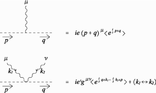
Figure 1: Vertices in Lorentz-invariant, scalar NCQED. Wavy lines for photon and dashed lines for charged scalar.

Photon self-energy diagrams as shown in Fig. 2 sum up to

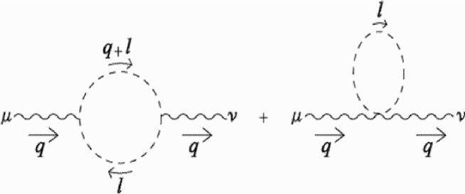
Figure 2: Photon self-energy diagrams in scalar QED.

$$i\Pi_{b(2)}^{\mu\nu}(q) = e^{2}\int\!\frac{d^{4}l}{(2\pi)^{4}}\big{[}\frac{(2l+q)^{\mu}(2l+q)^{\nu}}{(l^{2}-m^{2}+i\epsilon)((l+q)^{2}-m^{2}+i\epsilon)}\langle e^{\frac{i}{2}l\wedge q}\rangle\langle e^{\frac{i}{2}q\wedge l}\rangle$$ (16)

$$\hskip 54.06006pt-\frac{2g^{\mu\nu}}{l^{2}-m^{2}+i\epsilon}\langle e^{-iq\wedge l}\rangle\big{]},$$

where $q$ is the momentum of the external photon and $l$ the loop momentum. By writing

$$\langle e^{-iq\wedge l}\rangle=\langle e^{\frac{i}{2}q\wedge l}\rangle^{2}+[\langle e^{-iq\wedge l}\rangle-\langle e^{\frac{i}{2}q\wedge l}\rangle^{2}]$$ (17)

in the second term in (16) we can show that the contribution from the square bracket in (17) vanishes in the new UV limit. (See Appendix B.) We may therefore write using Feynman parameter

$$i\Pi_{b(2)}^{\mu\nu}(q) = i\stackrel{{\scriptstyle\!\!\!(1)}}{{\Pi_{b(2)}^{\mu\nu}}}(q)+i\stackrel{{\scriptstyle\!\!\!(2)}}{{\Pi_{b(2)}^{\mu\nu}}}(q),$$

$$i\stackrel{{\scriptstyle\!\!\!(1)}}{{\Pi_{b(2)}^{\mu\nu}}}(q) = 2e^{2}\int_{0}^{1}\!dx\int\!\frac{d^{4}l}{(2\pi)^{4}}\frac{2l^{\mu}l^{\nu}-g^{\mu\nu}(l^{2}-\Delta)}{(l^{2}-\Delta+i\epsilon)^{2}}V^{2}(q,l),$$

$$i\stackrel{{\scriptstyle\!\!\!(2)}}{{\Pi_{b(2)}^{\mu\nu}}}(q) = e^{2}(q^{\mu}q^{\nu}-q^{2}g^{\mu\nu})\int_{0}^{1}\!dx(1-2x)^{2}\int\!\frac{d^{4}l}{(2\pi)^{4}}\frac{V^{2}(q,l)}{(l^{2}-\Delta+i\epsilon)^{2}},$$ (18)

where $\Delta=-q^{2}x(1-x)+m^{2}$ and we have translated the integration variable. Since the extra vertex factor $V^{2}(q,l)$ depends on $q^{2},l^{2}$ as well as $q\cdot l$ by Lorentz invariance, we cannot replace $l^{\mu}l^{\nu}\to(1/4)g^{\mu\nu}l^{2}$ in the integrand of $\stackrel{{\scriptstyle\!\!\!(1)}}{{\Pi_{b(2)}^{\mu\nu}}}(q)$ as usually done in the symmetric integration. Consequently, we cannot conclude that the amplitude $\stackrel{{\scriptstyle\!\!\!(1)}}{{\Pi_{b(2)}^{\mu\nu}}}(q)$ is proportional to the metric tensor and, hence, exhibits quadratic divergence.
To evaluate the integral (18) we make Wick rotation,

$$l^{0} = il_{E}^{4},\quad{\boldsymbol{l}}={\boldsymbol{l}}_{E},$$

$$q^{0} = iq_{E}^{4},\quad{\boldsymbol{q}}={\boldsymbol{q}}_{E}.$$ (19)

Since the theory involves another parameter $\theta^{\mu\nu}$ carrying Lorentz indices, we must also perform Wick rotation

$$\theta^{0i}\to-i\theta_{E}^{4i},\;\;\;\theta^{ij}\to\theta_{E}^{ij},$$ (20)

such that

$$p\wedge l=p_{E}\wedge_{E}l_{E}\equiv\sum_{\mu,\nu=1,2,3,4}(p_{E})_{\mu}\theta_{E}^{\mu\nu}(l_{E})_{\nu}.$$ (21)

This is dictated by Lorentz invariance of $V(q,l)$. Then the amplitude (18) becomes in Euclidean metric with $g_{E}^{\mu\nu}=-\delta^{\mu\nu}$,

$$\stackrel{{\scriptstyle\!\!\!(1)}}{{\Pi_{b(2)}^{\mu\nu}}}(q_{E}) = 2e^{2}\int_{0}^{1}\!dx\int\!\frac{d^{4}l_{E}}{(2\pi)^{4}}\frac{2l_{E}^{\mu}l_{E}^{\nu}+g_{E}^{\mu\nu}(l_{E}^{2}+\Delta_{E})}{(l_{E}^{2}+\Delta_{E})^{2}}V^{2}(q_{E},l_{E}),$$

$$\stackrel{{\scriptstyle\!\!\!(2)}}{{\Pi_{b(2)}^{\mu\nu}}}(q) = e^{2}(q_{E}^{\mu}q_{E}^{\nu}+q_{E}^{2}g_{E}^{\mu\nu})\int_{0}^{1}\!dx(1-2x)^{2}\int\!\frac{d^{4}l_{E}}{(2\pi)^{4}}\frac{V^{2}(q_{E},l_{E})}{(l_{E}^{2}+\Delta_{E})^{2}},$$ (22)

where $\Delta_{E}=q_{E}^{2}x(1-x)+m^{2}$. Put

$$\int\!\frac{d^{4}l_{E}}{(2\pi)^{4}}\frac{l_{E}^{\mu}l_{E}^{\nu}}{(l_{E}^{2}+\Delta_{E})^{2}}V^{2}(q_{E},l_{E}) = C_{1}g_{E}^{\mu\nu}+C_{2}q_{E}^{\mu}q_{E}^{\nu},$$

$$\int\!\frac{d^{4}l_{E}}{(2\pi)^{4}}\frac{1}{l_{E}^{2}+\Delta_{E}}V^{2}(q_{E},l_{E}) = C_{3},$$ (23)

where $C_{1,2,3}$ are functions of invariant $q_{E}^{2}$. For Gaussian weight function which we employ in what follows, they are given by (see Appendix A)

$$C_{1}(-q_{E}^{2}) = -\frac{1}{32\pi^{2}}\int_{0}^{\infty}\!ds\frac{\sqrt{s}e^{-s\Delta}}{\big{(}\sqrt{s+A_{E}q_{E}^{2}}\big{)}^{5}},$$

$$C_{2}(-q_{E}^{2}) = \frac{1}{32\pi^{2}}A_{E}\int_{0}^{\infty}\!ds\frac{e^{-s\Delta}}{\sqrt{s}\big{(}\sqrt{s+A_{E}q_{E}^{2}}\big{)}^{5}},$$

$$C_{3}(-q_{E}^{2}) = \frac{1}{16\pi^{2}}\int_{0}^{\infty}\!ds\frac{e^{-s\Delta}}{\sqrt{s}\big{(}\sqrt{s+A_{E}q_{E}^{2}}\big{)}^{3}},$$ (24)

with $A_{E}=\frac{a^{4}}{2}\frac{\langle{\bar{\theta}}_{E}^{\,2}\rangle}{24}$. It follows that

$$2C_{1}(-q_{E}^{2})+C_{3}(-q_{E}^{2})=2C_{2}(-q_{E}^{2})q_{E}^{2}.$$ (25)

Substituting this equation with (23) into (22) yields

$$\stackrel{{\scriptstyle\!\!\!(1)}}{{\Pi_{b(2)}^{\mu\nu}}}(q_{E}) = 2e^{2}(q_{E}^{\mu}q_{E}^{\nu}+q_{E}^{2}g_{E}^{\mu\nu})\int_{0}^{1}\!dx(2C_{2}(-q_{E}^{2})),$$

$$\stackrel{{\scriptstyle\!\!\!(2)}}{{\Pi_{b(2)}^{\mu\nu}}}(q) = e^{2}(q_{E}^{\mu}q_{E}^{\nu}+q_{E}^{2}g_{E}^{\mu\nu})\int_{0}^{1}\!dx(1-2x)^{2}C_{4}(-q_{E}^{2}),$$ (26)

where we have defined

$$C_{4}(-q_{E}^{2})=\int\!\frac{d^{4}l_{E}}{(2\pi)^{4}}\frac{1}{(l_{E}^{2}+\Delta_{E})^{2}}V^{2}(q_{E},l_{E})=\frac{1}{16\pi^{2}}\int_{0}^{\infty}\!ds\frac{\sqrt{s}e^{-s\Delta_{E}}}{(\sqrt{s+A_{E}q_{E}^{2}})^{3}}.$$ (27)

Analytic continuation back to Minkowski metric gives

$$\stackrel{{\scriptstyle\!\!\!(1)}}{{\Pi_{b(2)}^{\mu\nu}}}(q) = 2e^{2}(q^{\mu}q^{\nu}-q^{2}g^{\mu\nu})\int_{0}^{1}\!dx(2C_{2}(q^{2})),$$

$$\stackrel{{\scriptstyle\!\!\!(2)}}{{\Pi_{b(2)}^{\mu\nu}}}(q) = e^{2}(q^{\mu}q^{\nu}-q^{2}g^{\mu\nu})\int_{0}^{1}\!dx(1-2x)^{2}C_{4}(q^{2}),$$ (28)

where $C_{i}(q^{2})(i=1,2,3,4)$ are obtained from $C_{i}(-q_{E}^{2})$ by $q_{E}^{2}\to-q^{2}$ and $A_{E}\to A=\frac{a^{4}}{2}\frac{\langle{\bar{\theta}}^{\,2}\rangle}{24}>0$. Thus the piece $\stackrel{{\scriptstyle\!\!\!(1)}}{{\Pi_{b(2)}^{\mu\nu}}}$ also becomes transverse as does $\stackrel{{\scriptstyle\!\!\!(2)}}{{\Pi_{b(2)}^{\mu\nu}}}$. This well-come situation is obtained without cancellation in our Lorentz-invariant NCQED. Unfortunately, however, this continuation process brings about a new problem. The problem arises because, although the functions $C_{i}(-q_{E}^{2})$ are finite for $a^{4}q_{E}^{2}\neq 0$, the functions $C_{i}(q^{2})$ are not well-defined for $a^{4}q^{2}\geq 0$. This is due to the presence of IR singularities in $C_{i}(-q_{E}^{2})$. In this respect see, also, the next section.
To avoid them we may modify $C_{i}(q^{2})$ to cutoff at the lower limit of the integration region. As explained in I we instead take the regularized functions

$$C_{2}(q^{2},\Lambda^{2})=\frac{1}{32\pi^{2}}A\int_{0}^{\infty}\!ds\frac{e^{-s\Delta-\frac{1}{s\Lambda^{2}}}}{\sqrt{s}\big{(}\sqrt{s-Aq^{2}}\big{)}^{5}},$$

$$C_{4}(q^{2},\Lambda^{2})=\frac{1}{16\pi^{2}}\int_{0}^{\infty}\!ds\frac{\sqrt{s}e^{-s\Delta-\frac{1}{s\Lambda^{2}}}}{\big{(}\sqrt{s-Aq^{2}}\big{)}^{3}}.$$ (29)

The cutoff factor $e^{-\frac{1}{s\Lambda^{2}}}$ is introduced to avoid the singularity at $s=Aq^{2}$ by taking the new UV limit (7) and the parameter $\Lambda$ is qualified to be called UV cutoff because it effectively cuts off the lower limit of Schwinger’s $s$-integration. Since $C_{2}$ goes like $A\Lambda^{4}/(32\pi^{2})$ in the new UV limit, we impose the condition

$$\Lambda^{2}a^{2}\to 0$$ (30)

to eliminate it since $A$ is proportional to $a^{4}$. In other words, the first term in (18) vanishes in the new UV limit supplemented with (30) as in other regularizations. The new UV limit of $C_{4}$ turns out to be given by

$$\mathop{\rm lim}_{\Lambda^{2}\to\infty,a^{2}\to 0,\Lambda^{2}a^{2}:{\rm fixed}}\;C_{4}(q^{2},\Lambda^{2}) = \mathop{\rm lim}_{\Lambda^{2}\to\infty}\,\frac{1}{8\pi^{2}}K_{0}\big{(}2\sqrt{\Delta/\Lambda^{2}}\big{)},$$ (31)

where $K_{0}$ is the modified Bessel function of the second kind. Subtraction at $q^{2}=0$ leads to

$$\Pi_{b(2),R}^{\mu\nu}(q) = \stackrel{{\scriptstyle\!\!\!(2)}}{{\Pi_{b(2),R}^{\mu\nu}}}(q)=\frac{\alpha}{4\pi}(q^{\mu}q^{\nu}-q^{2}g^{\mu\nu})\int_{0}^{1}\!dx(1-2x)^{2}\ln{\big{(}\frac{m^{2}}{\Delta}\big{)}}.$$ (32)

This is the renormalized photon self-energy amplitude obtained through NC regularization and the same as obtained in other gauge-invariant regularizations.
Let us now consider the Maxwell sector. In order to consistently quantize the gauge field in NCQED it is necessary to introduce the ghost fields, $c,{\bar{c}}$, and the Nakanishi-Lautrup field $B$ such that the full action is BRST-invariant.[14, 9] We use the Feynman rules of Ref. 9) as shown in Fig. 3 and choose the Feynman-’t Hooft gauge.

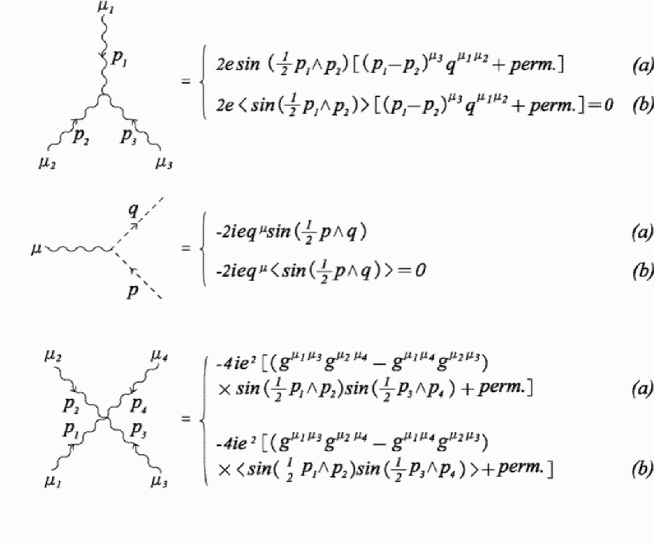
Figure 3: Feynman rules in the Maxwell sector of NCQED (a) and Lorentz-invariant NCQED (b). Wavy line represents photon and dashed line with arrow ghost.

Note that there exist no three-point vertices in the Lorentz-invariant NCQED if the action (13) is employed, because $\langle\sin{(\frac{1}{2}p\wedge q)}\rangle=0$. Consequently, ghosts decouple and there is only one more contribution to the photon self energy, the tadpole diagram.
The tadpole diagram as shown in Fig. 4 is given by

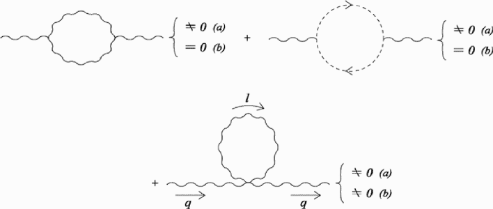
Figure 4: Photon self-energy diagrams in the Maxwell sector of NCQED. All diagrams contribute in NCQED (a), while only tadpole diagram has to be considered in Lorentz-invariant NCQED (b).

$$i\Pi_{\rm tadpole(2)}^{\mu\nu}(q) = -12e^{2}g^{\mu\nu}\int\!\frac{d^{4}l}{(2\pi)^{4}}\frac{1}{l^{2}+i\epsilon}\langle\sin^{2}{(\frac{1}{2}q\wedge l)}\rangle$$ (33)

$$= -6e^{2}g^{\mu\nu}\big{[}\int\!\frac{d^{4}l}{(2\pi)^{4}}\frac{1}{l^{2}+i\epsilon}-\int\!\frac{d^{4}l}{(2\pi)^{4}}\frac{1}{l^{2}+i\epsilon}\langle\cos{(q\wedge l)}\rangle\big{]},$$

where $q$ denotes the external photon momentum. As shown in I the new UV limit of the tadpole diagram is proportional to $a^{4}\Lambda^{4}$ and vanishes if we impose the condition (30). All contributions arising from non-Abelian nature of Lorentz-invariant NC Maxwell action (13) with ghost and gauge-fixing terms included disappear at least at one-loop order. In conclusion NC regularization with (30) gives rise to the renormalized one-loop photon self-energy in scalar QED given by (32) in accordance with other regularization schemes.

3 Vacuum polarization in QED

This section is devoted to a compact presentation of our previous[1] treatment of vacuum polarization in NC regularization scheme comparing with Pauli-Villars-Gupta and dimensional regularizations. The basic mathematical formulae we needed in I have repeatedly been used in the previous section and are collected in the Appendix A.
According to (2) the matter sector of the Lorentz-invariant NCQED is defined by the action

$${\hat{S}}_{\rm D} = \int\!d^{4}xd^{6}\theta W(\theta)\big{[}{\bar{\psi}}(x)(i\gamma^{\mu}\partial_{\mu}-M)\psi(x)+e{\bar{\psi}}(x)*\gamma^{\mu}A_{\mu}(x)*\psi(x)\big{]}.$$ (34)

The spinor is subject to the $\ast$-gauge transformation as in (9) and has the same covariant derivative,

$$\psi(x) \to {}^{\hat{g}}\psi(x)=U(x)*\psi(x),\;\;\;U(x)*U^{{\dagger}}(x)=U^{{\dagger}}(x)*U(x)=1,$$

$$D_{\mu}\psi(x) = \partial_{\mu}\psi(x)-ieA_{\mu}(x)*\psi(x).$$ (35)

The gauge field $A_{\mu}$ transforms as in (10). The discrete symmetries of Lorentz-invariant NCQED can be shown as in Ref. 16) in which we assumed fields to depend on $x$ as well as $\theta$. What we need in the present case is to delete the additional ‘dependence’ of fields on $\theta$.
Using the action (34) the vacuum polarization tensor in Lorentz-invariant NCQED is given by (see Fig. 5)

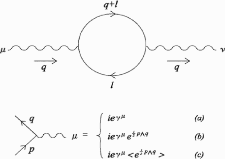
Figure 5: Vacuum polarization. Wavy lines for photon and solid lines for fermion. Vertices in QED (a), NCQED (b) and Lorentz-invariant NCQED (c).

$$i\Pi_{f(2)}^{\mu\nu}(q) = (ie)^{2}(-1)\int\!\frac{d^{4}l}{(2\pi)^{4}}{\rm Tr}\big{[}\gamma^{\mu}\frac{i}{l{\raise 0.8pt\hbox{$\!\!\!/$}}-M+i\epsilon}\gamma^{\nu}\frac{i}{q{\raise 0.8pt\hbox{$\!\!\!/$}}+l{\raise 0.8pt\hbox{$\!\!\!/$}}-M+i\epsilon}\big{]}\langle e^{\frac{i}{2}q\wedge l}\rangle\langle e^{\frac{i}{2}l\wedge q}\rangle,$$ (36)

where $q$ is the external photon momentum and $l$ the loop momentum. The vacuum polarization tensor in QED and NCQED is given by (36) without the extra vertex factors. It is denoted $\Pi_{f(2)}^{\mu\nu}(q)_{0}$ below. Computing the Dirac trace and translating the integration variable we have a similar expression like the scalar case,

$$\Pi_{f(2)}^{\mu\nu}(q) = \stackrel{{\scriptstyle\!\!\!(1)}}{{\Pi_{f(2)}^{\mu\nu}}}(q)+\stackrel{{\scriptstyle\!\!\!(2)}}{{\Pi_{f(2)}^{\mu\nu}}}(q),$$

$$i\stackrel{{\scriptstyle\!\!\!(1)}}{{\Pi_{f(2)}^{\mu\nu}}}(q) = -4e^{2}\int_{0}^{1}\!dx\int\!\frac{d^{4}l}{(2\pi)^{4}}\frac{2l^{\mu}l^{\nu}-g^{\mu\nu}(l^{2}-\Delta)}{(l^{2}-\Delta+i\epsilon)^{2}}V^{2}(q,l),$$

$$i\stackrel{{\scriptstyle\!\!\!(2)}}{{\Pi_{f(2)}^{\mu\nu}}}(q) = 4e^{2}(q^{\mu}q^{\nu}-q^{2}g^{\mu\nu})\int_{0}^{1}\!dx2x(1-x)\int\!\frac{d^{4}l}{(2\pi)^{4}}\frac{V^{2}(q,l)}{(l^{2}-\Delta+i\epsilon)^{2}},$$ (37)

with $\Delta=-q^{2}x(1-x)+M^{2}$. Before computing ‘non-transverse’ part $\stackrel{{\scriptstyle\!\!\!(1)}}{{\Pi_{f(2)}^{\mu\nu}}}\!\!(q)$ in NC regularization, let us first consider it in Pauli-Villars-Gupta and dimensional regularizations when no extra vertex factors appear as in QED and NCQED. Put

$$I^{\mu\nu}(q,M) = -i\int\!\frac{d^{4}l}{(2\pi)^{4}}\frac{2l^{\mu}l^{\nu}-g^{\mu\nu}(l^{2}-\Delta)}{(l^{2}-\Delta+i\epsilon)^{2}}$$ (38)

$$= \int\!\frac{d^{4}l_{E}}{(2\pi)^{4}}\frac{2l_{E}^{\mu}l_{E}^{\nu}-g_{E}^{\mu\nu}(-l_{E}^{2}-\Delta)}{(l_{E}^{2}+\Delta)^{2}},$$

where we have made Wick rotation. It is integrated over $x$ from 0 to 1 to give $\stackrel{{\scriptstyle\!\!\!(1)}}{{\Pi_{f(2)}^{\mu\nu}}}\!\!(q)_{0}$ apart from a constant. By symmetric integration $l^{\mu}l^{\nu}\to(1/4)g^{\mu\nu}l^{2}$ in the first integrand (or $l_{E}^{\mu}l_{E}^{\nu}\to-(1/4)g_{E}^{\mu\nu}l_{E}^{2}$ in the second integrand). Using Schwinger representation we obtain

$$I^{\mu\nu}(q,M) = g_{E}^{\mu\nu}\int_{0}^{\infty}\!dss\int\!\frac{d^{4}l}{(2\pi)^{4}}(\frac{1}{2}l_{E}^{2}+\Delta)e^{-s(l_{E}^{2}+\Delta)}$$ (39)

$$= -g_{E}^{\mu\nu}\frac{1}{16\pi^{2}}\int_{0}^{\infty}\!ds\frac{\partial}{\partial s}\big{(}\frac{1}{s}e^{-s\Delta)}\big{)}=-g_{E}^{\mu\nu}\frac{1}{16\pi^{2}}\frac{1}{s}e^{-s\Delta}|_{s=0}^{s=\infty}.$$

The lower limit does not exist (provided $\Delta$ is assumed to be positive). Pauli-Villars-Gupta regularization to cure this defect consists of replacing the integral $I^{\mu\nu}(q,M)$ with $I^{\mu\nu}_{reg}(q)=\sum_{i=0,1,2}C_{i}I^{\mu\nu}(q,M_{i})$ such that $\sum_{i=0,1,2}C_{i}=0$ and $\sum_{i=0,1,2}C_{i}M_{i}^{2}=0$, where $C_{0}=1,M_{0}=M$. It follows that $I^{\mu\nu}_{reg}(q)=0$ because

$$I^{\mu\nu}_{reg}(q) = g_{E}^{\mu\nu}\frac{1}{16\pi^{2}}\sum_{i=0,1,2}C_{i}\big{(}\frac{1}{s}e^{-s\Delta_{i}}\big{)}|_{s=0}$$ (40)

$$= g_{E}^{\mu\nu}\frac{1}{16\pi^{2}}\sum_{i=0,1,2}C_{i}\big{(}\frac{1}{s}+q^{2}x(1-x)-M_{i}^{2}\big{)}|_{s=0}=0.$$

On the other hand, dimensional regularization extends dimensions 4$\to n$ in which case $l^{\mu}l^{\nu}\to(1/n)g^{\mu\nu}l^{2}$ by symmetric integration. Then we have again using Schwinger representation

$$I_{4\to n}^{\mu\nu}(q,M) = g_{E}^{\mu\nu}\int\!\frac{d^{n}l_{E}}{(2\pi)^{n}}\frac{(1-\frac{2}{n})l_{E}^{2}+\Delta}{(l_{E}^{2}+\Delta)^{2}}$$ (41)

$$= g_{E}^{\mu\nu}\frac{1}{\Gamma(n/2)(4\pi)^{n/2}}$$

$$\hskip 14.22636pt\times\int_{0}^{\infty}\!ds\big{(}(1-2/n)\Gamma(n/2+1)s^{-n/2}+\Delta\Gamma(n/2)s^{-n/2+1}\big{)}e^{-s\Delta}=0,$$

where we have used $\Gamma(z+1)=z\Gamma(z)$. In either case we regularize $\stackrel{{\scriptstyle\!\!\!(1)}}{{\Pi_{f(2)}^{\mu\nu}}}\!\!(q)_{0}$ to zero satisfying gauge invariance.
On the contrary, NC regularization ‘dispenses’, in a sense, with the above regularization. We directly integrates the amplitudes (37) for Gaussian weight function, which turn out to be finite for $a^{4}q^{2}<0$. The procedure is already illustrated in scalar QED and detailed in I. By Wick rotation (19) through (21) we obtain (see (28))

$$\stackrel{{\scriptstyle\!\!\!(1)}}{{\Pi_{f(2)}^{\mu\nu}}}\!\!(q) = -4e^{2}(q^{\mu}q^{\nu}-q^{2}g^{\mu\nu})\int_{0}^{1}\!dx(2C_{2}(q^{2})),$$

$$\stackrel{{\scriptstyle\!\!\!(2)}}{{\Pi_{f(2)}^{\mu\nu}}}\!\!(q) = 4e^{2}(q^{\mu}q^{\nu}-q^{2}g^{\mu\nu})\int_{0}^{1}\!dx2x(1-x)C_{4}(q^{2}).$$ (42)

Since $C_{2,4}(q^{2})$ are finite for $a^{4}q^{2}<0$, (42) give finite, transverse vacuum polarization tensor in Lorentz-invariant NCQED (34) in the same region. At first sight this conclusion seems to differ from that of the known regularizations, $\stackrel{{\scriptstyle\!\!\!(1)}}{{\Pi_{f(2)}^{\mu\nu}}}\!\!(q)_{0}\to 0$, in QED. However, it is possible to fill up this apparent difference by noting that the commutative limit $a\to 0$ cannot be interchangeable with UV limit $\Lambda\to\infty$, that is, they must be taken simultaneously according to the new UV limit (7) with the condition (30). To be more precise we replace $C_{2,4}(q^{2})$ by the regularized functions (29) and take the new UV limit (7) with (30). It can then be shown in exactly the same way as in scalar QED that the piece $\stackrel{{\scriptstyle\!\!\!(1)}}{{\Pi_{f(2)}^{\mu\nu}}}\!\!(q)$ vanishes, leaving the well-known result after subtraction at $q^{2}=0$,

$$\Pi_{f(2),\lower 1.2pt\hbox{{\scriptsize${R}$}}}^{\mu\nu}(q) = (q^{\mu}q^{\nu}-q^{2}g^{\mu\nu})\big{(}-\frac{2\alpha}{\pi}\big{)}\int_{0}^{1}\!dxx(1-x)\ln{\big{(}\frac{M^{2}}{\Delta}\big{)}}.$$ (43)

The Maxwell sector is the same as in scalar QED and need not be repeated here. (See also I.)

4 One-loop gluon self-energy in $U(N)$ gauge theory

In this section we consider $U(N)$ gauge theory without matter. The basic field variable in the theory is $U(N)$ gauge field $A_{\mu}(x)=\sum_{A=0\cdots N^{2}-1}T_{A}A_{\mu}^{A}(x)$, where $T_{A},A=0,1,\cdots,N^{2}-1$ denote $U(N)$ generators with

$$[T_{A},T_{B}] = if_{ABC}T_{C},$$

$$\{T_{A},T_{B}\} = d_{ABC}T_{C},$$

$${\rm Tr}T_{A}T_{B} = \frac{1}{2}\delta_{AB}.$$ (44)

Following Ref. 15) we label $SU(N)$ components by small letters, say, $a=1,2,\cdots,N^{2}-1$. The structure constant $f_{ABC}$ equals $f_{abc}$ for $SU(N)$ components and $f_{0BC}=f_{A0C}=0$. The gauge field transforms as

$$A_{\mu}(x) \to {}^{g}A_{\mu}(x)=U(x)*A_{\mu}(x)*U^{{\dagger}}(x)+\frac{i}{g}U(x)*\partial_{\mu}U^{{\dagger}}(x),$$ (45)

$$U(x)*U^{{\dagger}}(x)=U^{{\dagger}}(x)*U(x)=1.$$

This gauge transformation mixes $U(1)$ component $A_{\mu}^{0}$ with $SU(N)$ ones $A_{\mu}^{a}$. NC non-Abelian gauge field strength takes of the same form as that in (11),

$$F_{\mu\nu}(x) = \partial_{\mu}A_{\nu}(x)-\partial_{\nu}A_{\mu}(x)-ig[A_{\mu}(x),A_{\nu}(x)]_{*},$$ (46)

where the nonlinear term is decomposed as follows.

$$[A_{\mu}(x),A_{\nu}(x)]_{*} \equiv A_{\mu}(x)*A_{\nu}(x)-A_{\nu}(x)*A_{\mu}(x)$$ (47)

$$= \frac{1}{2}\sum_{A,B=0,1,\cdots,N^{2}-1}(A_{\mu}^{A}(x)*A_{\nu}^{B}(x)-A_{\nu}^{B}(x)*A_{\mu}^{A}(x))\{T_{A},T_{B}\}$$

$$+\frac{1}{2}\sum_{a,b=1,\cdots,N^{2}-1}(A_{\mu}^{a}(x)*A_{\nu}^{b}(x)+A_{\nu}^{b}(x)*A_{\mu}^{a}(x))[T_{a},T_{b}].$$

To obtain the last term we used the relation $f_{0BC}=f_{A0C}=0$. Consequently, only in the Moyal bracket term appears the zeroth component. The fact that (47) contains not only the commutators but also the anti-commutators of generators explicitly demonstrates that $U(1)$ is not decoupled from $SU(N)$ in the field strength.
Lorentz-invariant, gauge-fixed action of NC $U(N)$ YM is given by

$${\hat{S}} = \int\!d^{4}xd^{6}\theta W(\theta){\rm Tr}\big{[}-\displaystyle{{1\over 4}}F_{\mu\nu}(x)*F^{\mu\nu}(x)-\frac{1}{2\xi}(\partial_{\mu}A^{\mu})^{2}+\frac{1}{2}(i{\bar{c}}*\partial_{\mu}D^{\mu}c-\partial_{\mu}D^{\mu}c*{\bar{c}})\big{]},$$ (48)

where covariant derivative of the ghost field is given by

$$D_{\mu}c=\partial_{\mu}c-ig[A_{\mu},c]_{*}.$$ (49)

Our prescription leading to the above action is based on (2) using gauge-fixed action of NC $U(N)$ YM in Ref.16). We employ Feynman-’t Hooft gauge $\xi=1$ as in §2. Feynman rules for NC $U(N)$ gauge theory without $\theta$-integration are given in Refs. 15) and 17). We need Feynman rules derived from (48). They are simply given by integrating those in Refs. 15) and 17) over $\theta$ at each vertex. The result is displayed in Fig. 6.

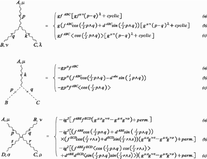
Figure 6: Feynman rules in $U(N)$ Yang-Mills (a), NC $U(N)$ Yang-Mills (b) and Lorentz-invariant $U(N)$ Yang-Mills. Wavy lines for gauge bosons and dashed lines with arrow for ghosts.

It is seen that $\theta$-integration helps decouple $U(1)$ from $SU(N)$ in all three-point vertices. This implies, in particular, that the zeroth component of ghost field completely decouples from the theory. On the other hand, $U(1)$ gauge boson couples to $SU(N)$ gauge boson only through 4-point vertex with the extra vertex factor carrying $\langle\sin{\frac{1}{2}(p\wedge q)}\sin{\frac{1}{2}(r\wedge s)}\rangle$ where $p,q,r,s$ are momenta flowing into the vertex.
One-loop self-energy correction of $SU(N)$ gauge boson is given by the sum of diagrams as shown in Fig. 7.

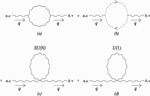
Figure 7: One-loop gluon self-energy diagrams. (a), (b), (c) contain only $SU(N)$ loops, while $U(1)$ circulates in the loop (d) in Lorentz-invariant NC $U(N)$ YM.

Ignoring the last diagram Fig. 7(d) for the moment and replacing the extra vertex factor $\langle\cos^{2}{\frac{1}{2}(l\wedge q)}\rangle$ in the tadpole diagram with $\langle\cos{\frac{1}{2}(l\wedge q)}\rangle^{2}$, we find the following result in terms of the invariant functions defined by (24) and (27):

$${\rm Fig.~{}7(a)} = \frac{1}{2}g^{2}f_{acd}f_{bcd}\int\!d^{4}l\frac{-i}{l^{2}+i\epsilon}\frac{-i}{(l+q)^{2}+i\epsilon}[g^{\mu\rho}(q-l)^{\sigma}+g^{\rho\sigma}(q+2l)^{\mu}+g^{\sigma\mu}(-2q-l)^{\rho}]$$

$$\times[\delta^{\nu}_{\;\;\rho}(l-q)_{\sigma}+g_{\rho\sigma}(-q-2l)^{\nu}+\delta_{\sigma}^{\;\;\nu}(2q+l)_{\rho}]\langle\cos{\frac{1}{2}(l\wedge q)}\rangle^{2}$$

$$= -\frac{i}{2}g^{2}C_{2}(SU(N))\delta_{ab}\int_{0}^{1}\!dx\big{[}g_{E}^{\mu\nu}\{2C_{3}(-q_{E}^{2})+q_{E}^{2}(4x^{2}-10x+8)C_{4}(-q_{E}^{2})-10C_{1}(-q_{E}^{2})\}$$

$$\hskip 136.5733pt+q_{E}^{\mu}q_{E}^{\nu}\{-10C_{2}(-q_{E}^{2})-(10x^{2}-10x-2)C_{4}(-q_{E}^{2})\}\big{]}$$

$${\rm Fig.~{}7(b)} = (-1)g^{2}f_{acd}f_{bdc}\int\!d^{4}l\frac{i}{l^{2}+i\epsilon}\frac{i}{(l+q)^{2}+i\epsilon}(l+q)^{\mu}l^{\nu}\langle\cos{\frac{1}{2}(l\wedge q)}\rangle^{2}$$

$$= -ig^{2}C_{2}(SU(N))\delta_{ab}\int_{0}^{1}\!dx\big{[}g_{E}^{\mu\nu}C_{1}(-q_{E}^{2})+q_{E}^{\mu}q_{E}^{\nu}(C_{2}(-q_{E}^{2})-x(1-x)C_{4}(-q_{E}^{2}))\big{]},$$

$${\rm Fig.~{}7(c)} = \frac{1}{2}(-ig)^{2}f_{acd}f_{bdc}\int\!d^{4}l\frac{-i}{l^{2}+i\epsilon}6g^{\mu\nu}\langle\cos{\frac{1}{2}(l\wedge q)}\rangle^{2}$$ (50)

$$= ig^{2}C_{2}(SU(N))\delta_{ab}3g_{E}^{\mu\nu}\int_{0}^{1}\!dx\big{[}C_{3}(-q_{E}^{2})+q_{E}^{2}(2x^{2}-3x+1)C_{4}(-q_{E}^{2})\big{]},$$

where $C_{2}(SU(N))$ is the second Casimir. Using the identity (25) to eliminate $C_{1,3}$ in favor of $C_{2}$, we obtain

$$i\Pi_{g(2)}^{\mu\nu,ab}(q_{E}) \equiv {\rm Fig.~{}7(a)}+{\rm Fig.~{}7(b)}+{\rm Fig.~{}7(c)}=ig^{2}C_{2}(SU(N))\delta_{ab}(q_{E}^{\mu}q_{E}^{\nu}+q_{E}^{2}g_{E}^{\mu\nu})\pi_{(2)}(-q_{E}^{2}),$$

$$\pi_{(2)}(-q_{E}^{2}) = \int_{0}^{1}\!dx[4C_{2}(-q_{E}^{2})+(4x^{2}-4x-1)C_{4}(-q_{E}^{2})].$$ (51)

Analytic continuation back to Minkowski metric finally gives

$$\Pi_{g(2)}^{\mu\nu,ab}(q) = g^{2}C_{2}(SU(N))\delta_{ab}(q^{\mu}q^{\nu}-q^{2}g^{\mu\nu})\pi_{(2)}(q^{2}),$$

$$\pi_{(2)}(q^{2}) = \int_{0}^{1}\!dx[4C_{2}(q^{2})+(4x^{2}-4x-1)C_{4}(q^{2})].$$ (52)

Consequently, the amplitude $\Pi_{g(2)}^{\mu\nu,ab}(q)$, which is finite for $a^{4}q^{2}<0$, becomes transverse as in QED. As we have seen in §2, IR singularity in $C_{2,4}(-q_{E}^{2})$ is eliminated by employing the regularized functions (27) which lead, in the new UV limit under the condition (30), to $C_{2}\to 0$ and $C_{4}\to(1/8\pi^{2})K_{0}(2\sqrt{\Delta/\Lambda^{2}})$ (see (31)). Hence, $\pi_{(2)}(q^{2})$ exhibits log divergence as should be the case. Subtraction at $q^{2}=-\mu^{2}$ yields

$$\Pi_{g(2),R}^{\mu\nu,ab}(q) = \frac{g^{2}}{4\pi}C_{2}(SU(N))\delta_{ab}(q^{\mu}q^{\nu}-q^{2}g^{\mu\nu})\pi_{(2),R}(q^{2}),$$

$$\pi_{(2),R}(q^{2}) = \int_{0}^{1}\!dx(4x^{2}-4x-1)\ln{\big{(}\frac{\mu^{2}}{-q^{2}}\big{)}}=-\frac{5}{3}\ln{\big{(}\frac{\mu^{2}}{-q^{2}}\big{)}}.$$ (53)

The diagram as shown in Fig. 7(d), in which $U(1)$ gauge boson circulates in the loop, gives

$${\rm Fig.~{}7(d)} = -3g^{2}\frac{2}{N}\delta_{ab}g^{\mu\nu}\int\!\frac{d^{4}l}{(2\pi)^{4}}\frac{1}{l^{2}+i\epsilon}\langle\sin^{2}{\frac{1}{2}(q\wedge l)}\rangle.$$ (54)

This is essentially equal to (33). As noted there the new UV limit of (54) vanishes upon using the condition (30). To sum up one-loop self-energy amplitude of $SU(N)$ gauge boson is given by (53) which include only $SU(N)$ gauge bosons circulating in the loop.
As for $U(1)$ gauge boson one-loop self-energy diagrams are given by Figs. 8(a) and 8(b) where $SU(N)$ loop and $U(1)$ loop are considered, respectively;

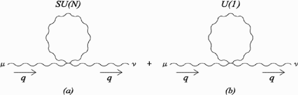
Figure 8: One-loop $U(1)$ gluon self-energy diagrams with $SU(N)$ (a) and $U(1)$ (b) loops, respectively.

$${\rm Fig.~{}8(a)} = -6g^{2}g^{\mu\nu}\int\!\frac{d^{4}l}{(2\pi)^{4}}\frac{1}{l^{2}+i\epsilon}\langle\sin^{2}{\frac{1}{2}(q\wedge l)}\rangle,$$

$${\rm Fig.~{}8(b)} = -\frac{6}{N}g^{2}g^{\mu\nu}\int\!\frac{d^{4}l}{(2\pi)^{4}}\frac{1}{l^{2}+i\epsilon}\langle\sin^{2}{\frac{1}{2}(q\wedge l)}\rangle.$$ (55)

Both of them vanish in the new UV limit with the condition (30). That is, $U(1)$ decouples from $SU(N)$ in the one-loop approximation for the self-energy diagram.

5 Discussions

We have presented several model calculations in the previous[1] and this papers that NC regularization works in non-gauge and gauge theories. The scenario of the method is based on the observation that, since UV divergence in QFT is renormalized away, the commutative limit of our Lorentz-invariant NCQFT must exhibit IR divergences to be subtracted off, if the IR limit and the commutative limit cannot be distinguishable. Indeed, one cannot discriminate the two limits as far as one-loop self-energy diagrams in Lorentz-invariant NCQFT are concerned. Moreover, it is important to recognize that the two limits have invariant meanings. Lorentz invariance unravels the hitherto-unknown aspect of the IR/UV mixing.
As remarked in I and reemphasized in §1 of this paper our use of Lorentz-invariant NCQFT as a means of the regularization in QFT is motivated to understand the IR/UV mixing in an invariant way. The elimination of the IR singularity is necessitated to make sense the Lorentz-invariant NCQFT quantum mechanically. There is alternative approach[10, 12] to the Lorentz-invariant NCQED using Seiberg-Witten map.[3] It tries to look for small effects arising from the nonvanishing small value of the fundamental length $a$. In this approach Feynman rules in the theory are the same as those of the commutative fields, regarding the Lorentz-invariant NCQED as an effective field theory. There is no vertex factor like $V(p,q)$ as introduced in §2.
Considering this possibility we may argue that the Lorentz-invariant NCQFT has dual roles. On one hand, it provides a kind of regularization by taking the new UV limit in which we let $a\to 0$. On the other hand, we seek for new physical effects by allowing $a$ to remain finite but extremely small with only known Feynman rules being encountered.
We have not yet checked consistency on the decoupling of $U(1)$ from $SU(N)$ since evaluation of multi-points vertices and higher-loops are still beyond our present ability. For instance, one may suppose that our one-loop calculation indicates different running of $U(1)$ and $SU(N)$ coupling constants, which may clash with $\ast$-gauge invariance. On the other hand, one may also suppose that, if $SU(N)$ is not broken as color, $U(1)$ is neither broken as $U(1)_{em}$. We shall study these and other problems including renormalization program in our scheme step by step.

Appendix A Some mathematical formulae

We collect here some mathematical formulae used in §2 and §3 from I. For typographical reason we omit the index $E$ and work in Euclidean metric, $g^{\mu\nu}=-\delta^{\mu\nu},\mu,\nu=1,2,3,4,$ with $q\cdot l=q^{4}l^{4}+{\boldsymbol{q}}\cdot{\boldsymbol{l}}$.
The definition (23) reads in this notation

$$\int\!\frac{d^{4}l}{(2\pi)^{4}}\frac{l^{\mu}l^{\nu}}{(l^{2}+\Delta)^{2}}V^{2}(q,l) = C_{1}g^{\mu\nu}+C_{2}q^{\mu}q^{\nu},$$ (56)

$$\int\!\frac{d^{4}l}{(2\pi)^{4}}\frac{1}{l^{2}+\Delta}V^{2}(q,l) = C_{3}.$$ (57)

To evaluate $l$-integral it is necessary to determine the extra vertex factor $V(q,l)$. Since there is no guiding principle to determine the weight function, we employ the simplest, namely, Gaussian weight function:

$$w({\bar{\theta}})=\frac{1}{\pi^{3}}e^{-b[({\bar{\theta}}^{41})^{2}+({\bar{\theta}}^{42})^{2}+({\bar{\theta}}^{43})^{2}+({\bar{\theta}}^{12})^{2}+{\bar{\theta}}^{23})^{2}+({\bar{\theta}}^{31})^{2}]},b>0.$$ (58)

The extra vertex factor is then determined[12] as

$$V(p,l) = e^{-\frac{A}{2}[l^{2}p^{2}-(p\cdot l)^{2}]},$$ (59)

where

$$A=\frac{a^{4}}{2}\frac{\langle{\bar{\theta}}^{\,2}\rangle}{24}$$ (60)

with $\langle{\bar{\theta}}^{\,2}\rangle=6/b$. Since $C_{1,2}$ are functions of invariant $q^{2}$ only, we calculate the integral in (A$\cdot$ 1) by choosing the 4-th direction in $l$-space as pointing to the vector $q$ so that

$$q = (0,0,0,q),\quad l=(l^{1},l^{2},l^{3},l^{4}),$$

$$l^{4} = l\cos{\theta_{1}},\quad l^{3}=l\sin{\theta_{1}}\cos{\theta_{2}},$$

$$l^{2} = l\sin{\theta_{1}}\sin{\theta_{2}}\cos{\theta_{3}},\quad l^{1}=l\sin{\theta_{1}}\sin{\theta_{2}}\sin{\theta_{3}}.$$ (61)

The $\mu=\nu=4$ component of (A$\cdot$ 1) is then given by

$$\int\!\frac{d^{4}l}{(2\pi)^{4}}\frac{l^{2}\cos^{2}{\theta_{1}}}{(l^{2}+\Delta)^{2}}e^{-Al^{2}q^{2}\sin{\theta_{1}}} = -C_{1}+C_{2}q^{2},$$ (62)

while the $\mu=\nu=3$ component determines $C_{1}$,

$$\int\!\frac{d^{4}l}{(2\pi)^{4}}\frac{l^{2}\sin^{2}{\theta_{1}}\cos^{2}{\theta_{2}}}{(l^{2}+\Delta)^{2}}e^{-Aq^{2}l^{2}\sin^{2}{\theta_{1}}} = -C_{1}.$$ (63)

The $l$-integrals in (A$\cdot$ 7) and (A$\cdot$ 8) can easily be done in the spherical coordinates using Schwinger representation to yield

$$C_{1} = -\frac{1}{32\pi^{2}}\int_{0}^{\infty}\!ds\frac{\sqrt{s}e^{-s\Delta}}{\big{(}\sqrt{s+Aq^{2}}\big{)}^{5}},$$

$$C_{2} = \frac{1}{32\pi^{2}}A\int_{0}^{\infty}\!ds\frac{e^{-s\Delta}}{\sqrt{s}\big{(}\sqrt{s+Aq^{2}}\big{)}^{5}}.$$ (64)

On the other hand, the definition for $C_{3}$ leads to the result

$$C_{3} = \int\!\frac{d^{4}l}{(2\pi)^{4}}\frac{1}{l^{2}+\Delta}e^{-Aq^{2}l^{2}\sin^{2}{\theta_{1}}}$$ (65)

$$= \frac{1}{16\pi^{2}}\int_{0}^{\infty}\!ds\frac{e^{-s\Delta}}{\sqrt{s}\big{(}\sqrt{s+Aq^{2}}\big{)}^{3}}.$$

The relation

$$2C_{1}+C_{3}=2C_{2}q^{2}$$ (66)

follows immediately. Equations (A$\cdot$ 9), (A$\cdot$ 10) and (A$\cdot$ 11) are reported in (24) and (25).
The integrals considered so far are divergent as $a\to 0$ where $V(q,l)\to 1$. This divergent behavior is transferred to IR singularity as seen from (A$\cdot$ 9) and (A$\cdot$ 10). It may not be uninteresting to see what happens for ‘convergent’ integrals at $a=0$ ignoring Ward-Takahashi identity. We expect that they possess no IR singularity at all and the relation (A$\cdot$ 11) breaks down.
To be definite we consider the following ‘convergent’ integrals

$$\int\!\frac{d^{4}l}{(2\pi)^{4}}\frac{l^{\mu}l^{\nu}}{(l^{2}+\Delta)^{4}}V^{2}(q,l) = D_{1}g^{\mu\nu}+D_{2}q^{\mu}q^{\nu},$$ (67)

$$\int\!\frac{d^{4}l}{(2\pi)^{4}}\frac{1}{(l^{2}+\Delta)^{3}}V^{2}(q,l) = D_{3}.$$ (68)

We use the same function (A$\cdot$ 4) for $V(q,l)$. The result turns out to be

$$D_{1} = -\frac{1}{32\pi^{2}}\frac{1}{\Gamma(4)}\int_{0}^{\infty}\!ds\frac{s^{5/2}e^{-s\Delta}}{\big{(}\sqrt{s+Aq^{2}}\big{)}^{5}},$$

$$D_{2} = \frac{1}{32\pi^{2}}\frac{1}{\Gamma(4)}A\int_{0}^{\infty}\!ds\frac{s^{3/2}e^{-s\Delta}}{\big{(}\sqrt{s+Aq^{2}}\big{)}^{5}},$$

$$D_{3} = \frac{1}{16\pi^{2}}\frac{1}{\Gamma(3)}\int_{0}^{\infty}\!ds\frac{s^{3/2}e^{-s\Delta}}{\big{(}\sqrt{s+Aq^{2}}\big{)}^{3}}.$$ (69)

These integrals have no IR singularity because they are convergent at $a=0$. Instead of the relation (A$\cdot$ 11) we find

$$6D_{1}+D_{3}=6D_{2}q^{2}.$$ (70)

The absence of IR singularity makes the relation (A$\cdot$ 11) change into a different one like (A$\cdot$ 15). The transversality of the amplitudes $\stackrel{{\scriptstyle\!\!\!(1)}}{{\Pi_{b,f(2)}^{\mu\nu}}}(q)$ can be proven only for (18) and (37).
There is a similar circumstance in dimensional regularization. Although the integral

$$I^{\mu\nu}=\int\!\frac{d^{n}l}{(2\pi)^{n}}\frac{2l^{\mu}l^{\nu}-g^{\mu\nu}(l^{2}-\Delta)}{(l^{2}-\Delta+i\epsilon)^{2}}$$ (71)

vanishes in dimensional regularization as shown in §3, the integral

$$J^{\mu\nu}=\int\!\frac{d^{n}l}{(2\pi)^{n}}\frac{2l^{\mu}l^{\nu}-g^{\mu\nu}(l^{2}-\Delta)}{(l^{2}-\Delta+i\epsilon)^{4}}$$ (72)

does not vanish for $n\to 4$.

Appendix B Tadpole contribution to photon self-energy

Set $\Delta V=\langle e^{-iq\wedge l}\rangle-\langle e^{\frac{i}{2}q\wedge l}\rangle^{2}$. We prove that the integral

$$K(q^{2})=i\int\!\frac{d^{4}l}{(2\pi)^{4}}\frac{\Delta V}{l^{2}-m^{2}+i\epsilon}$$ (73)

vanishes in the new UV limit. Wick rotation gives

$$K(-q_{E}^{2})=\int\!\frac{d^{4}l_{E}}{(2\pi)^{4}}\frac{\Delta V_{E}}{l_{E}^{2}+m^{2}}.$$ (74)

Using (A$\cdot$ 4) we have

$$K(-q_{E}^{2}) = \int\!\frac{d^{4}l_{E}}{(2\pi)^{4}}\frac{1}{l_{E}^{2}+m^{2}}[e^{-2A_{E}(q_{E}^{2}l_{E}^{2}-(q_{E}\cdot l_{E})^{2})}-e^{-A_{E}(q_{E}^{2}l_{E}^{2}-(q_{E}\cdot l_{E})^{2})}],$$ (75)

which is cast into the form by (A$\cdot$ 10)

$$K(-q_{E}^{2}) = \frac{1}{16\pi^{2}}\int_{0}^{\infty}\!ds\big{[}\frac{e^{-sm^{2}}}{\sqrt{s}\big{(}\sqrt{s+2A_{E}q_{E}^{2}}\big{)}^{3}}-\frac{e^{-sm^{2}}}{\sqrt{s}\big{(}\sqrt{s+A_{E}q_{E}^{2}}\big{)}^{3}}\big{]}.$$ (76)

Analytic continuation back to Minkowski metric introduces the UV cutoff as in (29),

$$K(q^{2},\Lambda^{2}) = \frac{1}{16\pi^{2}}\int_{0}^{\infty}\!ds\big{[}\frac{e^{-sm^{2}-\frac{1}{s\Lambda^{2}}}}{\sqrt{s}\big{(}\sqrt{s-2Aq^{2}}\big{)}^{3}}-\frac{e^{-sm^{2}-\frac{1}{s\Lambda^{2}}}}{\sqrt{s}\big{(}\sqrt{s-Aq^{2}}\big{)}^{3}}\big{]}.$$ (77)

We may expand the integrand with respect to $Aq^{2}$ and take the new UV limit (7) to obtain

$$\mathop{\rm lim}_{\Lambda^{2}\to\infty,a^{2}\to 0,\Lambda^{2}a^{2}:{\rm fixed}}\;K(q^{2},\Lambda^{2})=\mathop{\rm lim}_{\Lambda^{2}\to\infty,a^{2}\to 0,\Lambda^{2}a^{2}:{\rm fixed}}\;\frac{3}{32\pi^{2}}Aq^{2}2(m^{2}\Lambda^{2})K_{2}\big{(}2\sqrt{m^{2}/\Lambda^{2}}\big{)}$$ (78)

which vanishes by the condition (30) since $K_{2}(z)\to 2/z^{2}$ as $z\to 0$. This proves that the square-bracketed term in (17) can be neglected in the new UV limit with (30).
We may skip the above detailed calculation by noting that $\Delta V$ behaves like $a^{4}l^{2}$ for small $a$. Inserting $a^{4}l^{2}$ for $\Delta V$ in (B$\cdot$ 1) we find $a^{4}$ times a quartic divergent integral, that is, $K(q^{2})$ is essentially given by $a^{4}\Lambda^{4}$ which vanishes by the condition (30).

Appendix C Tadpole contribution to $SU(N)$ gluon self-energy

Here put $\Delta^{\prime}V=\langle\cos^{2}{\frac{1}{2}l\wedge q}\rangle-\langle\cos{\frac{1}{2}l\wedge q}\rangle^{2}$. We prove that the integral

$$L(q^{2})=i\int\!\frac{d^{4}l}{(2\pi)^{4}}\frac{\Delta^{\prime}V}{l^{2}+i\epsilon}$$ (79)

vanishes in the new UV limit. Using $\Delta^{\prime}V=1-\langle\sin^{2}{\frac{1}{2}l\wedge q}\rangle-\langle\cos{\frac{1}{2}l\wedge q}\rangle^{2}$ and noting the fact that (33) vanishes in the new UV limit, we may replace $\Delta^{\prime}V$ in (79) with $\Delta^{\prime\prime}V=1-\langle\cos{\frac{1}{2}l\wedge q}\rangle^{2}$ to get

$$L(q^{2})=i\int\!\frac{d^{4}l}{(2\pi)^{4}}\frac{\Delta^{\prime\prime}V}{l^{2}+i\epsilon}.$$ (80)

Wick rotation and use of (65) yields

$$L(q^{2},\Lambda^{2})=\int\!\frac{d^{4}l_{E}}{(2\pi)^{4}}\frac{1}{l_{E}^{2}}|_{\Lambda^{2}}-\frac{1}{16\pi^{2}}\int_{0}^{\infty}\!ds\frac{e^{-\frac{1}{s\Lambda^{2}}}}{\sqrt{s}\big{(}\sqrt{s-Aq^{2}}\big{)}^{3}},$$ (81)

where we regulated the integrals. This goes like $a^{4}\Lambda^{4}$ in the new UV limit and can be neglected if we impose the condition (30). This allows us to evaluate the tadpole diagram for $S(N)$ gluon self-energy by replacing the extra vertex factor $\langle\cos^{2}{\frac{1}{2}(l\wedge q)}\rangle$ with $\langle\cos{\frac{1}{2}(l\wedge q)}\rangle^{2}$ as done in §4. Similar proof goes through for all other tadpole diagrams.

References

- [1] K. Morita, ‘A New Gauge-Invariant Regularization Scheme Based On Lorentz-Invariant Noncommutative Quantum Field Theory’, hep-th/0312080. This paper is referred to as I in the text.
- [2] See, for instance, M. R. Douglas and N. A. Nekrasov, ‘Noncommutative field theory’, Rev. Mod. Phys. 73(2001), 1029, (hep-th/0106048); R. J. Szabo, ‘Quantum Field Theory on Noncommutative Spaces’, Phys. Rep. 378(2003), 207, (hep-th/0109162).
- [3] N. Seiberg and E. Witten, ‘String Theory and Noncommutative Geometry’, J. High Energy Phys. 09 (1999), 032. (hep-th/9908142).
- [4] S. Minwalla, M. Van Raamsdonk and N. Seiberg, ‘Noncommutative Perturbative Dynamics’, JHEP 02, 035. (hep-th/9912072); see, also, N. Seiberg, L. Susskind and N. Toumbas, J. High Energy Phy. 06(2000), 044. (hep-th/0005015); Y. Kinar, G. Lifshytz and J. Sonnenschein, ‘UV/IR connection, a matrix perspective’, JHEP 02, 0108:001 (hep-th/0105089) and references therein.
- [5] J. Gomis and T. Mehen, ‘Space-Time Noncommutative Field Theories And Unitarity’; Nucl. Phys. B591(2000), 265. (hep-th/0005129)
- [6] H. S. Snyder, Phys. Rev. 71 (1947), 38; C. N. Yang, Phys. Rev. 72 (1947), 874.
- [7] S. Doplicher, K. Fredenhagen and J. E. Roberts, Phys. Lett. B 331 (1994), 39; Commun. Math. Phys. 172 (1995), 187.
- [8] T. Filk, Phys. Lett. B 376 (1996), 53.
- [9] M. Hayakawa, ‘Perturbative analysis on infrared and ultraviolet aspects of noncommutative QED on ’, Phys. Lett. B478 (2000), 394. (hep-th/9912167).
- [10] C. E. Carlson, C. D. Carone and N. Zobin, ‘Noncommutative Gauge Theory without Lorentz Violation’, Phys. Rev. D66(2002), 075001. (hep-th/0206035).
- [11] B. Juro, L. Möller, S. Shraml, P. Schupp, and J. Wess, ‘Construction of non-Abelian gauge theories on noncommutative spaces’, hep-th/0104153, Eur. Phys. J. C 21 (2001), 383.
- [12] K. Morita, ‘Lorentz-Invariant Non-Commutative QED’, Prog. Theor. Phys. 108(2002), 1099. (hep-th/0209243).
- [13] H. Kase, K. Morita, Y. Okumura, and E. Umezawa, ‘Lorentz-Invariant Non-Commutative Space-Time Based On DFR Algebra’, Prog. Theor. Phys. 109(2003), 664. (hep-th/0212176).
- [14] C. P. Martín and D. Sánchez-Ruiz, ‘One-loop UV Divergent Structure of Yang-Mills Theory on noncommutative ’, Phys. Rev. Lett. B83 (1999), 476. (hep-th/990377).
- [15] A. Armoni, ‘Comments on perturbative dynamics of non-commutative Yang-Mills theory’, Nucl. Phys. B593 (2001), 229, (hep-th/0005208);
- [16] K. Morita, ‘Discrete Symmetries In Lorentz-Invariant Non-Commutative QED’, Prog. Theor. Phys. 110(2003), 1003. (hep-th/0309159).
- [17] L. Bonora and M. Salizzoni, ‘Renormalization of noncommutative gauge theories’, Phys. Lett. B504 (2001), 80. (hep-th/0011088).