Expansion for the solutions of the Bogomolny equations on the torus

Abstract:

We show that the solutions of the Bogomolny equations for the Abelian Higgs model on a two-dimensional torus, can be expanded in powers of a quantity $\epsilon$ measuring the departure of the area from the critical area. This allows a precise determination of the shape of the solutions for all magnetic fluxes and arbitrary position of the Higgs field zeroes. The expansion is carried out to 51 orders for a couple of representative cases, including the unit flux case. We analyse the behaviour of the expansion in the limit of large areas, in which case the solutions approach those on the plane. Our results suggest convergence all the way up to infinite area.

1 Introduction

Topological defects play an important role in Particle Physics, Cosmology, and many areas of Condensed Matter Physics, like superconductivity, superliquid helium, etc. Minimum energy(action) configurations carrying topological charges arise as solutions of non-linear partial differential equations. In some situations, these solutions are not explicitly known, and one needs to make use of approximate analytical or numerical methods to study their structure and properties.

The Abelian Higgs model is one of the simplest models to study these ideas. It serves as a relativistic field theory extension of the Ginzburg-Landau description of a superconductor, in which a scalar field represents the condensate of Cooper pairs. In addition to superconductivity, modifications of the Abelian Higgs model have found applications in other domains of Physics, such as Cosmology (see for example Ref. vilenkin ). On a different level, the Abelian Higgs model acts as a simplified model in which to explore ideas and develop methods useful for non-abelian gauge theories. It illustrates phenomena such as spontaneously broken gauge symmetry, colour confinement, the dual Meissner effect, topological charges, and others, all of which play a role in our present understanding of Particle Physics.

Abrikosov abrikosov realised that superconductors contain string-like topological defects or configurations, which represent magnetic flux tubes. A corresponding stable stationary cylindrically-symmetric configuration of minimum energy per unit length of the Abelian Higgs model was discovered by Nielsen and Olesen no:vortice . Cutting a slice orthogonal to the direction of the string, we obtain a two-dimensional field configuration. Its stability arises from the fact that it possesses non-trivial topological charge. In this case, the topological charge is just the magnetic flux going through the plane which, for finite energy (per unit length) configurations, is quantised in multiple units of $2\pi$. Despite its conceptual simplicity, there is no explicit analytical expression for the unit magnetic-flux minimum energy configuration(the Nielsen-Olesen vortex).

The self-coupling constant of the scalar field $\lambda$ determines the ratio of photon to scalar field masses. There is a critical value of this coupling $\lambda_{c}$ (equal to one, in our units), separating the case of type I ($\lambda<\lambda_{c}$) and type II ($\lambda>\lambda_{c}$) superconductors Kramer:1966 ; Muller:1966 . Similarly to what happens with non-abelian gauge theories in 4 dimensions, Bogomolny Bogomolny:1975de discovered that (for $\lambda\geq\lambda_{c}$) the 2-dimensional energy of any configuration is bounded by a given constant times the absolute value of the topological charge. At the critical coupling $\lambda_{c}$, the bound is saturated by the solutions of a system of first order partial differential equations: the Bogomolny equations.

Solutions of the Bogomolny equations not only exist but, for $\lambda=\lambda_{c}$, exhaust all solutions of the two-dimensional field equations (energy extrema) Taubes1980cm . Furthermore, the space of solutions defines a manifold of dimension $2q$ Taubes:1980tm , where $q$ is the number of flux quanta. This is again very similar to the situation for self-duality equations in non-abelian gauge theories in 4 dimensions (4D). Indeed, a connection between both topics is known Taubes1980cm . Despite these properties, there are no explicit analytical expressions for these solutions. The unit flux cylindrically-symmetric solution was constructed as a power series in the radial coordinate by H. J. de Vega and F. A. Schaposnik deVega:1976mi . For higher fluxes, a solution is determined uniquely by the location of the $q$ zeroes (counted with multiplicity) of the Higgs field. These points can be interpreted as the position in the plane of $q$ unit-vortices. Since the energy does not depend on these positions (is given by the flux alone), one can think of these unit-vortices as non-interacting (This is not exactly true when one takes into account the kinetic terms in 4D). There are corresponding zero-modes associated with this degeneracy Weinberg:er . This contrasts with the situation for non-critical coupling. Numerical simulations rb:vortice and other methods tell us that when $\lambda>\lambda_{c}$, the interaction between vortices is repulsive, and there are no static solutions of the equations of motion for flux greater that $2\pi$ in the plane. On the other hand, if $\lambda<\lambda_{c}$ the interaction between vortices is attractive, and the solution of the equations of motion is a single vortex that carries all the flux (also called a “giant” vortex).

Certain problems require some knowledge of the structure of the solutions, and, in the absence of analytical expressions for them, one must rely upon approximate methods. Frequently these methods are specific to cylindrically symmetric solutions, or make use of specific ansatze. This is the case of the numerical methods of Ref. rb:vortice , for example. Other approximations are based on expansions in powers of certain quantities. We already cited the study of de Vega and Schaposnik deVega:1976mi for cylindrically-symmetric solutions. Similar expansions have been used to study excitations of the vortices in the type II superconducting phase Arodzycia .

In this paper we will present a new method to obtain the solutions of the Bogomolny equations on the 2-dimensional torus by means of an expansion in a parameter measuring the departure of the area from the critical area of $4q\pi$ (measured in units of the square correlation length). The method can be applied to obtain solutions of arbitrary flux and with Higgs zeroes at prescribed (but arbitrary) points. Truncating this expansion at a given order one obtains approximations to the solutions which tend to become worse with increasing area. However, as we will see, accessible truncations of the expansion give precise results even for large sizes, where the torus solutions approach those of the plane. Thus, although our primary goal is that of obtaining the solutions on the torus, it seems possible that problems pertaining to the plane can be addressed in this way too. Part of our motivation arises from the fact that a similar expansion was proposed to study self-dual Yang-Mills field configurations on the four dimensional torus GarciaPerez:2000yt . The present case is a simplified version of the 4D problem, and hence better suited for performing a more detailed convergence analysis.

The outline of the paper is as follows. In the next section the method will be presented. In the following one, we will apply it to the two simplest cases: The unit-flux vortex case and a flux=2 case with no circular symmetry. In both cases the expansion is carried out up to 51 orders. This enables us to do an analysis of convergence of the series for various sizes, including the infinite area case. Finally, in the last section, we present the conclusions and indicate prospects for future research. In addition, we have included an appendix describing a variant method with a quantum mechanical flavour. Although, less efficient than the method explained in section 2, it has several advantages over it, one being that, at the present stage, seems better suited for generalisation to the non-abelian self-duality study. It also has served as a test of the actual computed coefficients of the expansion, since they have been obtained with both methods and two independent codes.

2 Description of the method

In suitable units (unit charge and photon mass), the Lagrangian density of the abelian Higgs model in four-dimensional($4D$) Minkowski space-time, is given by:

$$\mathcal{L}=-\frac{1}{4}F_{\mu\nu}F^{\mu\nu}+\frac{1}{2}(D_{\mu}\phi)^{*}(D^{\mu}\phi)-\frac{\lambda}{8}(|\phi|^{2}-1)^{2}$$ (1)

where $\phi$ is a complex scalar field, and $D_{\mu}=\partial_{\mu}-iA_{\mu}$ is the covariant derivative with respect to $A_{\mu}$, the $U(1)$ gauge potential. This system is known abrikosov ; no:vortice ; Taubes:1980tm to possess static, $z$-independent (vortex like) solutions of the classical equations of motion. These configurations are local minima of the $2D$ energy, whose density is

$$\mathcal{E}=\frac{1}{4}F_{ij}F^{ij}+\frac{1}{2}|D_{i}\phi|^{2}+\frac{\lambda}{8}(|\phi|^{2}-1)^{2}$$ (2)

where Latin indices run over two spatial coordinates: $i,j,\dots=1,2$.

We will focus in the case in which the coupling $\lambda$ takes the critical value $\lambda_{c}=1$. Then, the second order (2D) differential equations of motion reduce to a set of first order ones (Bogomolny equations)Bogomolny:1975de . For positive flux and in our units these equations take the form:

$$(D_{1}+iD_{2})\phi=0$$ (3)

$$B=\frac{1}{2}(1-|\phi|^{2})$$ (4)

where $B$ is the (z-component of the) magnetic field.

Our goal is to study the solution to these Bogomolny equations for fields living in a $2D$ Torus (for an introduction to gauge fields on the torus seega:torus ). The appropriate mathematical description involves sections of a U(1) bundle. We will be working within a fixed trivialisation. The torus can be viewed as the quotient space of the plane ${\mathbb{R}}^{2}$ modulo the lattice $\Lambda$ generated by two linearly independent 2D vectors $e^{(1)}$, $e^{(2)}$. We assume that the torus is equipped with a flat Riemannian metric, which we will fix to be Euclidean. Within a specific trivialisation, the charged fields(sections) $\phi(x)\equiv\phi(x_{1},x_{2})$ are given by complex valued functions satisfying certain periodicity properties:

$$\phi(x+e^{(i)})=\Omega_{i}(x)\,\phi(x)$$ (5)

The $U(1)$ fields $\Omega_{i}(x)$ are the transition functions, which have to satisfy the following consistency conditions

$$\Omega_{1}(x+e^{(2)})\,\Omega_{2}(x)=\Omega_{2}(x+e^{(1)})\,\Omega_{1}(x)$$ (6)

The topological properties of the bundle, encoded in the transition functions, are associated with the first Chern class $c_{1}$. Its corresponding integer Chern number is known, and will be shown later, to physically correspond to the magnetic flux going through the torus in units of $2\pi$.

Without loss of generality we can choose the following specific form of the transition functions:

$$\Omega_{i}(x)=\exp\{\imath\pi\omega(e^{(i)},x)\}$$ (7)

where $\omega$ is an antisymmetric form. The consistency condition (6) forces
$\omega(e^{(1)},e^{(2)})\equiv q$ to take integer values. This is precisely the first Chern number mentioned previously.

Gauge fields are connections on this bundle. It is well known that the space of gauge fields is an affine space. The associated vector space is the space of 1-forms on the torus. Thus, we can decompose

$$A=A^{(0)}+\sigma$$ (8)

where $\sigma$ is a 1-form and $A^{(0)}$ is a specific connection. For the latter, it is natural to select a gauge field having constant field strength $f=F_{12}=-F_{21}$:

$$A^{(0)}_{i}(x)=-\frac{1}{2}F_{ij}x_{j}$$ (9)

Compatibility with the boundary conditions relates the antisymmetric matrix $F$ with $\omega$ as follows

$$F=2\pi\omega$$ (10)

which shows the relation between flux and Chern number. For the 1-form $\sigma$ we might use Hodge theorem and split it as a sum of of an exact, co-exact and a harmonic form:

$$A=\pi\omega(x,dx)+v+dg-\delta h$$ (11)

In components we might write

$$A_{i}(x)=A_{i}^{(0)}(x)+\partial_{i}g-\epsilon_{ij}\partial_{j}h+v_{i}$$ (12)

where $h$ and $g$ are real periodic functions and $v_{i}$ are constants (a representative of the harmonic forms on the torus). Although locally these constants are pure gauges, globally they are not. Their value influences Polyakov loops winding around the torus, which are gauge invariant quantities. In this way it is easy to realise that the $v_{i}$ can be considered elements of the dual torus ${\mathbb{R}}^{2}/\Lambda^{*}$. In addition, one can fix $h$ so that its integral over the torus vanishes ($\int d^{2}x\,h=0$).

Now we can return to the Bogomolny equations and express them in terms of $v_{i}$ and the periodic function $h$. For simplicity we will restrict to orthogonal periods $e^{(1)}=(l_{1},0)$, $e^{(2)}=(0,l_{2})$ (in appendix A we will study the general case). It is convenient to make use of complex coordinates:

$$z=\frac{x_{1}+ix_{2}}{2};\qquad\overline{z}=\frac{x_{1}-ix_{2}}{2}$$ (13a)

$$\partial=\partial_{1}-i\partial_{2};\qquad\overline{\partial}=\partial_{1}+i\partial_{2}$$ (13b)

$$\partial_{1}=\frac{1}{2}(\partial+\overline{\partial});\qquad\partial_{2}=\frac{1}{2i}(\partial-\overline{\partial})$$ (13c)

The notation is chosen so that $\partial z=\overline{\partial}\overline{z}=1$.

Similarly the vector potential can be expressed as a complex function $A=A_{1}-iA_{2}$ (with $\overline{A}=A_{1}+iA_{2}$). In this notation the Bogomolny equations take the form:

$$(\overline{\partial}-i\overline{A})\phi=0$$ (14a)

$$-\frac{i}{2}\left(\partial\overline{A}-\overline{\partial}A\right)=\frac{1}{2}(1-|\phi|^{2})$$ (14b)

Our specific parametrisation of the vector potential ($A^{(0)}=-if\overline{z}$) becomes:

$$A=\partial g-i\partial h+v-if\overline{z}$$ (15)

where $h$ and $g$ are periodic functions, and $v=v_{1}-iv_{2}$ is a complex constant. For the Higgs field we will use the following parametrisation

$$\phi={\mathcal{N}}e^{-h+ig}\chi$$ (16)

where $\chi$ is a normalised function (i.e. $\int_{\mathbb{T}^{2}}|\chi|^{2}d^{2}x=l_{1}l_{2}$), satisfying the same boundary conditions as $\phi$, and $\mathcal{N}$ is a normalisation constant. With this terminology the Bogomolny equations become:

$$(\overline{\partial}+fz)\chi=i\bar{v}\chi$$ (17a)

$$\partial\overline{\partial}h=\frac{1}{2}(1-2f-|{\mathcal{N}}|^{2}e^{-2h}|\chi|^{2})$$ (17b)

These equations can be solved sequentially. The first equation allows one to determine $\chi$, satisfying the correct boundary and normalisation conditions. This can be done analytically as will be shown in the next subsection. Once this is solved, we can use the second equation to solve for the periodic function $h$ and the normalisation $\mathcal{N}$. The equation is, however, a non-linear partial differential equation and the analytic solution is not known. For a particular value of the area $l_{1}l_{2}=4q\pi$, corresponding to $f=\frac{1}{2}$, a solution is given by $h=\mathcal{N}=0$. Our strategy consists in using $\epsilon=1-2f$ as a perturbative parameter. In what follows we will explain more precisely the procedure that we follow.

Since $h$ is periodic, we can use its Fourier decomposition:

$$h=\sum_{n_{1}n_{2}}h_{n_{1}n_{2}}e^{2\pi in_{1}x_{1}/l_{1}}e^{2\pi in_{1}x_{2}/l_{2}}$$ (18)

and expand the Fourier coefficients in a power series in $\epsilon$:

$$h_{n_{1}n_{2}}=\sum_{k=1}^{\infty}h_{n_{1}n_{2}}^{(k)}\epsilon^{k}$$ (19)

Similarly, we can write

$$|{\mathcal{N}}|^{2}=\sum_{k=1}^{\infty}\mathtt{A}_{k}\epsilon^{k}$$ (20)

The only additional input that we will need are the Fourier coefficients of $|\chi|^{2}$. Although in some cases it is interesting and possible to deal with Fourier coefficients which are series expansions in powers $\epsilon$, we will restrict here to the case in which these coefficients are independent of $\epsilon$ (but dependent on the aspect ratio $\tau=\frac{l_{2}}{l_{1}}$). The different situations will be clarified in the following subsection. Notice that our condition on $h$ fixes $h_{00}=0$. Alternatively, we might have taken $\mathcal{N}=1$, and allow for non-zero $h_{00}$, but our choice is more natural within our expansion.

To solve Eq. 17b we equate the Fourier coefficients of both sides of the equation order by order in $\epsilon$. The left-hand side takes the form

$$-(1-\epsilon)\xi(\tau,n_{1},n_{2})\sum_{k}h^{(k)}_{n_{1}n_{2}}\epsilon^{k}$$ (21)

where

$$\xi(\tau,n_{1},n_{2})=\frac{\pi\tau}{q}\left[n_{1}^{2}+\frac{n_{2}^{2}}{\tau^{2}}\right]$$ (22)

which vanishes for $n_{1}=n_{2}=0$. We remind the reader that $\tau=l_{2}/l_{1}$ and $q$ is the first Chern number.

To treat the right-hand side we first expand it in powers of $\epsilon$. To order $\epsilon$ the coefficient is given by $(1-\mathtt{A}_{1}|\chi|^{2})/2$. The coefficient of order $\epsilon^{N}$ (for $N>1$) is given by

$$-\frac{1}{2}\sum_{k=0}^{N-1}\mathtt{A}_{N-k}\left[\frac{(-2)^{k}}{k!}\sum_{\begin{array}[]{c}i_{1},{\ldots},i_{N-1}\\ /\sum_{s}si_{s}=k\end{array}}\binom{\sum_{s}i_{s}}{i_{1},{\ldots},i_{N-1}}{h^{(1)}}^{i_{1}}\cdots{h^{(N-1)}}^{i_{N-1}}\right]|\chi|^{2}$$ (23)

Now, using the Fourier coefficients of $|\chi|^{2}$ (see the following subsection), we can obtain the Fourier coefficients of the expression above by applying a series of convolutions. We will label these Fourier modes with the symbol $\mathcal{F}_{n_{1}n_{2}}^{(N)}$. These are functions of $\mathtt{A}_{i}(i=1,\dots,N)$, and $h^{(i)}(i=1,\dots,N-1)$. In order for the equation to have a solution it is necessary that $\mathcal{F}_{00}^{(N)}=0$. This can be regarded as an equation for $\mathtt{A}_{N}$. It allows to determine this coefficient uniquely in terms of $\mathtt{A}_{i}(i=1,\dots,N-1)$, and $h^{(i)}(i=1,\dots,N-1)$.

Finally, the equation allows one to obtain the Fourier coefficients $h^{(N)}_{n_{1}n_{2}}$ to order $\epsilon^{N}$ as follows:

$$h_{n_{1}n_{2}}^{(N)}=\left\{\begin{array}[]{ll}-\frac{\mathcal{F}_{n_{1}n_{2}}^{(N)}}{\xi(\tau,n_{1},n_{2})}+h_{n_{1}n_{2}}^{(N-1)}&n_{1}\neq 0\quad\mbox{or}\quad n_{2}\neq 0\\ 0&n_{1}=n_{2}=0\\ \end{array}\right.$$ (24)

This equation defines a recurrence which, starting from $h^{(0)}_{n_{1}n_{2}}=0$, enables the determination of the coefficients $h^{(k)}_{n_{1}n_{2}}$ uniquely. To order $\epsilon$, $\mathcal{F}_{n_{1}n_{2}}^{(1)}$ are the Fourier coefficients of $(1-\mathtt{A}_{1}|\chi|^{2})$. The vanishing of the $n_{1}=n_{2}=0$ coefficient and the normalisation condition for $\chi$ implies $A_{1}$=1. The coefficients $h_{n_{1}n_{2}}^{(1)}$ are then given by

$$h_{n_{1}n_{2}}^{(1)}=-(1-\delta_{n_{1}0}\delta_{n_{2}0})\frac{\mathcal{F}_{n_{1}n_{2}}^{(1)}}{\xi(\tau,n_{1},n_{2})}$$ (25)

Computing the coefficients to higher orders demands performing convolutions, which involve infinite sums over several integers. We do not have closed analytical expressions for them. In practice, however, the Fourier coefficients decrease very fast with the order, so that a truncation of these sums to a finite subset allows, as we will show later, the numerical determination of the coefficients to machine precision up to high orders in the expansion.

We emphasise that the previous procedure gives rise to a unique solution $h$. All the degrees of freedom associated to the space of solutions of the Bogomolny equations resides in the function $\chi$ which will be treated in the following subsection.

2.1 The function $\chi$

In this section we will solve the first Bogomolny equation, Eq. 17a. First of all we will analyse the dependence on $\bar{v}=v_{1}+\imath v_{2}$. It is easy to see that if $\chi_{\bar{v}}$ is the solution the equation for a value of $\bar{v}$, then a solution for $\bar{v}^{\prime}=\bar{v}+2ifa$ is given by

$$\chi_{\bar{v}^{\prime}}=e^{f(\overline{a}z-a\overline{z})}\chi_{\bar{v}}(z+a,\overline{z}+\overline{a})$$ (26)

Since the prefactor is simply a phase, it is clear that solutions corresponding to different values of $v$ represent solutions translated in space. Having this point in mind we can simply restrict from now on to $v=0$.

To solve Eq. 17a we define $\eta=e^{fz(\overline{z}-z)}\chi$. In terms of this function the first Bogomolny equation is equivalent to the condition of holomorphicity $\overline{\partial}\eta=0$. So $\eta=\eta(z)$ is an analytic function of the variable $z$. The boundary conditions for this function can be obtained from the ones of $\phi$ (Eq. 5), and are given by

$$\eta\left(z+\frac{l_{1}}{2}\right)=\eta(z)$$ (27a)

$$\eta\left(z+i\frac{l_{2}}{2}\right)=e^{-2ifl_{2}z+f\frac{l_{2}^{2}}{2}}\eta(z)$$ (27b)

These are the typical conditions satisfied by theta functions ww:analysis . We will now analyse the space of solutions in various cases.

For minimal flux $q=1$ $f=\frac{2\pi}{l_{1}l_{2}}$, it is easy to see that our function is given by

$$\eta=\left(\frac{2l_{2}}{l_{1}}\right)^{\frac{1}{4}}\vartheta_{3}\left(\frac{2\pi z}{l_{1}}|i\frac{l_{2}}{l_{1}}\right)$$ (28)

This, together with the normalisation condition, allows us to obtain the Fourier decomposition of $\chi^{2}$:

$$|\chi|^{2}=\sum_{n_{1},n_{2}}e^{-\frac{\xi(\tau,n_{1},n_{2})}{2}}e^{2\pi in_{1}x_{1}/l_{1}}e^{2\pi in_{2}x_{2}/l_{2}}(-1)^{n_{1}n_{2}}$$ (29)

where $\xi(\tau,n_{1},n_{2})$ is given by Eq. 22. From here it is trivial to obtain $\mathcal{F}_{n_{1}n_{2}}^{(1)}$ to initiate the iteration that determines $h$.

For flux $2\pi q$ the space of solutions is multiple dimensional. There are several alternative ways to characterise individual solutions. One possibility is to fix the position of the zeroes of $\chi$, which coincide with those of the Higgs field $\phi$. Then we can write

$$\eta\propto\vartheta_{3}\left(\frac{2\pi(z+z_{c}-\omega_{1})}{l_{1}}|i\frac{l_{2}}{l_{1}}\right)\vartheta_{3}\left(\frac{2\pi(z+z_{c}-\omega_{2})}{l_{1}}|i\frac{l_{2}}{l_{1}}\right)\cdots\vartheta_{3}\left(\frac{2\pi(z+z_{c}-\omega_{q})}{l_{1}}|i\frac{l_{2}}{l_{1}}\right)$$ (30)

where $\omega_{i}$ are complex constants, and $z_{c}=\frac{1}{4}(l_{1}+il_{2})$. This is a holomorphic function, and satisfies the correct boundary conditions provided

$$\sum_{i}\omega_{i}=qz_{c}$$ (31)

The function $\eta$ defined in this way has $q$ zeros located at the points $\omega_{i}$. Eq. 31 then specifies that the centre of mass of all the zeroes is located at the centre of the torus ($\frac{l_{1}}{2},\frac{l_{2}}{2}$). To shift the centre of mass one must choose $v\neq 0$.

An alternative description of the space of solutions follows naturally from the quantum mechanical formulation of appendix A. A basis of the space of holomorphic functions satisfying the same boundary conditions as $\eta(z)$ is given by:

$$\eta_{s}(z)=\vartheta\left[\begin{array}[]{c}s/q\\ 0\end{array}\right]\left(\frac{2\pi qz}{l_{1}}|iq\frac{l_{2}}{l_{1}}\right)\qquad(s=0,\dots,q-1)$$ (32)

where the symbols $\vartheta\left[\begin{array}[]{c}a\\ b\end{array}\right]$ denote Theta functions with rational characteristics:

$$\vartheta\left[\begin{array}[]{c}a\\ b\end{array}\right](z|\tau)=\sum_{n\in\mathbb{Z}}e^{i\pi\tau(n+a)^{2}}e^{2i(n+a)(z+b)}$$ (33)

The functions $\eta_{s}(z)$ have $q$ zeros located at

$$\left(\frac{l_{1}}{2q}(2k+1),\frac{l_{2}}{2}-\frac{s}{q}l_{2}\right)\qquad(k=0,\dots,q-1)$$ (34)

An arbitrary solution of the problem is given by a suitably normalised linear combination of $\eta_{s}(z)$: $\eta\propto\sum_{s}c_{s}\eta_{s}(z)$.

Now we can relate the two descriptions by relating the coefficients $c_{s}$ to the position of the zeroes $\omega_{i}$. We can construct a linear combination that possesses $q-1$ zeros at the (distinct) complex points $\omega_{i}$, $i=1,\dots,q-1$ by setting

$$\eta(z)\propto\left|\begin{array}[]{cccc}\eta_{0}(z)&\eta_{1}(z)&\cdots&\eta_{q-1}(z)\\ \eta_{0}(\omega_{1})&\eta_{1}(\omega_{1})&\cdots&\eta_{q-1}(\omega_{1})\\ \vdots&\vdots&\vdots&\vdots\\ \eta_{0}(\omega_{q-1})&\eta_{1}(\omega_{q-1})&\cdots&\eta_{q-1}(\omega_{q-1})\\ \end{array}\right|$$ (35)

General theorems about elliptic functions tell us that the remaining zero of this $\eta$ function is located at a point $\omega_{0}$ which enforces the centre-of-mass condition.

The coefficients

$$c_{s}=\varepsilon_{si_{1}\dots i_{q-1}}\eta_{i_{1}}(\omega_{1})\cdots\eta_{i_{q-1}}(\omega_{q-1})$$ (36)

give rise to coordinates in the manifold of solutions of the Bogomolny equations. Actually, they define coordinates in the submanifold defined by the centre of mass condition for the zeroes Eq. 31. Using properties of elliptic functions and the result of Taubes Taubes:1980tm one can easily see that this submanifold is diffeomorphic to $\mathbf{CP}^{q-1}$ and $c_{s}$ are homogeneous coordinates. One has to include $v$ to give coordinates over the whole manifold of solutions. Since the latter varies over a torus, we recover the fiber bundle structure described in Refs. Shah:1993us ; Nasir:1998 ; Nasir:1999 .

The formula relating the coordinates to the zeroes Eq. 36 fails if two or more zeroes coincide. To write the correct formula one has to substitute some rows of Eq. 35 with the values of the derivatives (up to order given by the degeneracy) of the functions $\eta_{s}$.

Finally, it is easy to obtain the Fourier coefficients of $|\chi|^{2}$, using the corresponding ones for theta functions with rational characteristics. The result is

$$|\chi|^{2}=\frac{1}{\sum_{s}|c_{s}|^{2}}\sum_{n_{1},n_{2}}e^{-\frac{\xi(\tau,n_{1},n_{2})}{2}}e^{i\pi\frac{n_{1}n_{2}}{q}}\left(\sum_{s}c_{s}c^{*}_{s+n_{1}}e^{2\pi i\frac{sn_{2}}{q}}\right)e^{2\pi in_{1}\frac{x_{1}}{l_{1}}}e^{2\pi in_{2}\frac{x_{2}}{l_{2}}}$$ (37)

where $c_{s}$ is given above.

In all our previous construction the position of the zeroes of the Higgs field have been fixed relative to the Torus lengths $l_{1},l_{2}$. One could, in principle, insist in fixing the position of the zeroes in units of the inverse photon mass. This amounts to taking the positions $\omega_{i}$ as functions of $\epsilon$. We might still use the previous formula but now one has

$$|\chi|^{2}=\sum_{k}C_{k}(x)\epsilon^{k}$$ (38)

The iterative solution of Eq. 17b given in the previous subsection must then be modified by combining the powers of $\epsilon$ from $|\chi|^{2}$ into the expansion.

3 Representative examples

In this section we will show the effectiveness of the method presented in the previous section, by applying it to two explicit examples. The first one is the standard $q=1$ case, which should converge towards the usual Nielsen-Olesen vortex with cylindrical symmetry when the Torus is big enough. An extensive analysis of convergence of the series for different volumes will be presented. The second example is a $q=2$ case which has no remnant continuous spatial symmetry. This is important since many alternative methods are specific to cylindrical symmetry.

3.1 $q=1$

We have applied the machinery explained in the previous section to the unit flux $q=1$ and unit aspect ratio $\tau=l_{2}/l_{1}=1$ case. The solution is unique up to translations. We have obtained the coefficients of the expansion $h_{n_{1}n_{2}}^{(k)}$ up to order $k=51$. Convolutions were performed by truncating the sums to Fourier modes in the range $|n_{i}|\leq n_{\rm\tiny max}$. This was a implemented using a FORTRAN 90 program running in a standard PC. Results up to $k=51$ required computation times around 100 hours.

We have, first of all, analysed the effect of truncation in the number $n_{\rm\tiny max}$ of Fourier modes used in convolutions on the value of the coefficients. We explored the cases $n_{\rm\tiny max}=10,14$ and $20$. We estimate the relative difference (difference over sum) in the coefficient $h_{n_{1}n_{2}}^{(k)}$ obtained from two different truncations 10-14 or 14-20. The difference is attributed to an error in the value for the smaller $n_{\rm\tiny max}$. The differences increase with $n_{i}$ and with $k$. However, even for the highest order ($k=51$) the relative difference between the results with $n_{\rm\tiny max}=14$ and $20$ is of the order of machine precision $10^{-16,-17}$ for all modes having $n_{i}<7$. For higher modes it is to be expected that the error is mostly due to an error in the values for $n_{\rm\tiny max}=14$, so the modes for $n_{\rm\tiny max}=20$ remain probably within machine precision for higher $n_{i}$. To analyse this we used the comparison 10-14 to try to understand the dependence of errors with $n_{i}$, $k$ and $n_{\rm\tiny max}$. It is to be expected that the error is proportional to (some power) of the size of the neglected terms $h_{n_{\rm\tiny max}n_{\rm\tiny max}}^{(k)}$. This fits nicely with the observed dependence of the relative difference

$$-3(1)-\frac{1270(30)}{k}+\max(n_{1},n_{2})\left(-0.15(6)+\frac{54(1)}{k}\right)$$ (39)

Our interpretation of the source of the errors suggest that the coefficients multiplying $\frac{1}{k}$ are proportional to $n^{2}_{\rm\tiny max}$. This allows us to scale the results to $n_{\rm\tiny max}=14$. Indeed, our data on the difference 14-20 is consistent with this interpretation, although there are few values of $k$ and $n_{i}$ to allow an analysis by itself. On the basis of these results, we conclude that, even at $k=51$, the coefficients obtained for $n_{\rm\tiny max}=20$ are correct up to machine (double) precision for $n_{i}\leq 14-15$.

Once the coefficients are obtained, one can reconstruct the Fourier modes of $h$, the magnetic field $B$ and the modulus of the Higgs field $|\phi|$ for arbitrary torus areas ${\cal A}=l_{1}l_{2}=\frac{4\pi}{1-\epsilon}$. Obviously, the precision of the truncated series depends on the value of $\epsilon$, decreasing as $\epsilon$ increases up to the infinite area case of $\epsilon=1$. Even for relatively large areas the shape of the reconstructed function looks qualitatively quite good. See for example Fig. 1,2, where we display the magnetic field for $\epsilon=0.9$, obtained from the Fourier modes ($|n_{i}|\leq 20$) computed with 51 orders in the expansion.

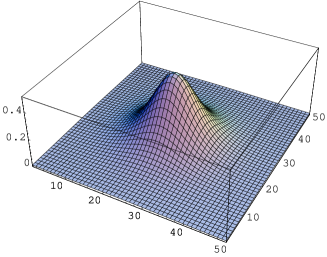
Figure 1: Shape of the magnetic field $B(x)$ obtained for $\epsilon=0.9$ with 51 orders in the expansion.

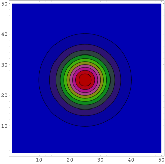
Figure 2: Contour plot of $B(x)$.

To go beyond the qualitative level and estimate the accuracy of the truncated series, we use the degree of satisfaction of the Bogomolny equation as a measure of the error. Thus, we compute the magnetic field $B(x)$ for various values of $\epsilon$ and compare it with the right-hand side of Eq. 4   $\frac{1}{2}(1-|\phi(x)|^{2})$. The latter is computed using the truncated expansion of $h$ and the parametrisation Eq. 16. More precisely we computed the $L_{2}$ and $L_{\infty}$ norm of the difference:

$$L_{2}(N,\epsilon)=\left(\frac{1}{l_{1}l_{2}}\int_{\mathbb{T}^{2}}dx\,\left[B(x)-\frac{1}{2}(1-|\phi(x)|^{2})\right]^{2}\right)^{1/2}\quad$$ (40a)

$$L_{\infty}(N,\epsilon)=\max_{x}\left\{\left|B(x)-\frac{1}{2}(1-|\phi(x)|^{2})\right|\right\}$$ (40b)

where $N$ is the maximal order in the expansion. We have analysed the $N$ and $\epsilon$ dependence of both quantities. Results are qualitatively the same for both, so we will choose $L_{2}$ to display. First, we will comment on the maximum precision, attained for $n=51$. For $\epsilon\leq 0.6$ the $L_{2}$ norm is compatible with zero within machine precision (order $10^{-16,-17}$). Beyond this value $L_{2}$ becomes sizable and increases, reaching $10^{-4}$ at $\epsilon=0.95$. For comparison we point out that with $N=1$ the value (at $\epsilon=0.95$) is $\mathcal{O}(10^{-2})$. Convergence is therefore slow in this case, but notice that the linear size of the box is 15 times the Debye screening length or 4.5 times the square root of the critical area.

Figure 3: $L_{2}(N,\epsilon)$ versus $N$ (in $\log_{10}$ scale) for $\epsilon=0.9$.

Figure 4: $a(\epsilon)$ versus $\epsilon$ compared to our best fit Eq. 3.5.

We performed a more systematic study by analysing the $N$ dependence for fixed value of $\epsilon$, in the range $0.1-0.95$. In this range the results are unaffected by the truncation in the number of Fourier modes $n_{\rm\tiny max}$. In all cases, we found that, beyond the first few orders, the dependence of $L_{2}(N,\epsilon)$ with $N$ oscillates around an exponential fall-off. As an example, we show in Fig. 3 the $\epsilon=0.9$ case . Therefore, we fitted $\log_{10}L_{2}$ data to the following linear function:

$$\log_{10}L_{2}(N,\epsilon)=a(\epsilon)N+b(\epsilon)$$ (41)

The parameter $a(\epsilon)$ is determined with errors reflecting the statistical and systematic uncertainties (range of fitting for example). Its value determines how the approximation improves when increasing the order $N$ in the expansion. Its negative value is an indication that the expansion is indeed convergent. Obviously as $\epsilon$ increases so does $a(\epsilon)$. This is displayed in Fig. 4. For a convergent series and small $\epsilon$ one expects

$$\log_{10}L_{2}(N,\epsilon)\approx(N+1)\log_{10}(\epsilon)+\log_{10}(c_{N})$$ (42)

and hence, $a(\epsilon)=\log_{10}(\epsilon)+\mbox{constant}+O(\epsilon)$. This is indeed the behaviour shown by the Fig. 3. Fitting $a(\epsilon)$ to a linear function of $\log_{10}\epsilon$ gives:

$$a(\epsilon)=1.022(5)\log_{10}\epsilon-0.0106(6)$$ (43)

Errors reflect the quality of the fit. Remarkably nothing seems to be happening at $\epsilon=1$, where the area diverges. Data cannot be taken directly at $\epsilon=1$ because they are severely affected by the truncation in the number of Fourier modes, but the behaviour up to $\epsilon=0.95$ shows no sign of a change of pattern and extrapolates to $a(1)<1$. Similar smooth behaviour is shown by $b(\epsilon)$. So we take our results as an indication that the series actually converges all the way up to $\epsilon=1$.

Within our spirit of identifying the $L_{2}$ (or $L_{\infty}$) norm of the equation with the error on the Higgs and magnetic field, we can use our data from a more practical viewpoint as an estimate of the number of terms required in the expansion to attain an a priori decided precision. An approximate formula can be derived from our data. If one is willing to compute the magnetic field with an error of $10^{-p}$ then the number of terms required in the expansion is given by:

$$n\approx\frac{1.83\epsilon+p-3.25}{0.01-1.02\log_{10}\epsilon}$$ (44)

Although the formula gives a finite number even for $\epsilon=1$, we stress once more that in practise at that very large volumes, truncation in the number of Fourier of terms would make the expansion increasingly computationally costly.

Now we will explore the implications of our expansion for large volumes. Our main assumption is that the solutions on the torus do converge to those on the plane. The convergence is expected to be fairly fast. A torus configuration is equivalent to a periodic array of vortices on the plane. However, vortices are exponentially localised objects so that if the period is large compared to the typical size of a vortex, the effect of the replicas is presumably very small. Now the convergence of the solution implies the following behaviour of the Fourier modes:

$$Y(\vec{p})\equiv\frac{\hat{B}(p)}{4\pi q}=\lim_{\epsilon\rightarrow 1}\xi(1,n_{1}(p),n_{2}(p))\,h_{n_{1}(p),n_{2}(p)}\,(-1)^{n_{1}(p)+n_{2}(p)}$$ (45)

where $\hat{B}(\vec{p})$ is the Fourier transform of the magnetic field on the plane. The limit is taken at fixed $p$ given by:

$$p^{2}\equiv|\vec{p}|^{2}=\xi\,(1-\epsilon)$$ (46)

where $\xi$ is given by Eq. 22. This means that as $\epsilon$ tends to 1, the integers $n_{i}(p)$ have to grow. If instead, we take the limit $\epsilon\rightarrow 1$ keeping $n_{i}$ fixed, the values should converge to $Y(0)=0.5$ irrespective of $n_{i}$. In our case ($q=1$), computing the value at $\epsilon=1$ using our 51 orders and $n_{1}=1$,$n_{2}=0$ we get $Y(0)=0.499947172199$. Worse results follow for higher modes ($0.499572$ for $n_{1}=n_{2}=1$, $0.465354$ for $n_{1}=2$, $n_{2}=1$, $0.387814$ for $n_{1}=n_{2}=2$, etc). The numerical agreement provides an additional hint that the expansion converges up to $\epsilon=1$. It also indicates a poorer convergence for larger $n_{i}$ (see later).

For $p$ non-zero, Eq. 45 and the expectation of fast convergence, suggests that tuning $\epsilon$ and $n_{i}$ in such a way that $p$ is fixed we should obtain similar values. Only $p$, the modulus of $\vec{p}$, matters due to the cylindrical symmetry of the $q=1$ solution on the plane. This is also satisfied by our expansion to a fairly high precision. For example, $Y(p)$ can be computed for $p^{2}=\pi/20$ using $\epsilon=0.975$ and $n_{1}=n_{2}=1$, or $\epsilon=0.95$ and $n_{1}=1,n_{2}=0$. From our expansion we get $0.39967$ and $0.39977$ respectively. This number is presumably very close ($<1\%$) to $Y(p)$ on the plane. Similarly for $p^{2}=\pi/10$ we get $0.326083$ and $0.326075$ from the same two modes and $\epsilon=0.95,0.9$ respectively. For $p^{2}=\pi/5$ we get $0.22627$ ($\epsilon=0.8$), $0.22676$ ($\epsilon=0.9$) and $0.22608$ ($\epsilon=0.95$). In this way we can use our expansion to compute the Fourier transform of the magnetic field for a vortex on the plane with a precision of a few percent.

Now we will try to extract the consequences of the convergence of the expansion for the Fourier modes to a universal function of $p$ as $\epsilon\rightarrow 1$. For very large $n_{i}$ (large $\xi$) we can compute $Y(p)$ by taking $\epsilon=1-p^{2}/\xi$. Thus,

$$Y(p)\approx-\xi\,(-1)^{n_{1}+n_{2}}\,h_{n_{1}n_{2}}(\epsilon)\approx-\xi\sum_{k=0}^{N}(-1)^{n_{1}+n_{2}}\,h_{n_{1}n_{2}}^{(k)}e^{-p^{2}\frac{k}{\xi}}$$ (47)

This suggests that for $\xi\rightarrow\infty$

$$h_{n_{1}n_{2}}^{(k)}\longrightarrow\frac{-1}{\xi^{2}}\,\varphi(k/\xi)\,(-1)^{n_{1}+n_{2}}$$ (48)

where the function $\varphi(y)$ satisfies

$$Y(p)=\int_{0}^{\infty}dy\,\varphi(y)\,e^{-p^{2}y}$$ (49)

Fourier transforming we get:

$$B(x)=\int_{0}^{\infty}\frac{dy}{y}\varphi(y)\,e^{-|\vec{x}|^{2}/(4y)}$$ (50)

One can test these considerations by computing approximants to $\varphi(y)$ by using Eq. 48 for finite $n_{i}$. In Fig. 5 we show the shape obtained from the coefficients $h_{n_{1}n_{2}}^{(k)}$. For any $y$ we plot only those values of $n_{i}$ such that $\xi\geq y/25$. The smoothness and small dispersion of values agrees with our expectations. We also investigated the way in which the limit is approached for large $\xi$. For example in Fig. 6 we plot $-\xi^{2}(-1)^{n_{1}+n_{2}}h_{n_{1}n_{2}}^{(k)}$ for different values of $n_{i}$ and a fixed value of $y=k/\xi=1/\pi$. The solid line is the result of a fit to a function of the form $a+\frac{b}{\xi}$. Similar behaviour obtains for other $y$ values. This analysis could be used to obtain a more precise estimation of the value $\varphi(y)$. For the time being we simply used the non-extrapolated shape shown in Fig. 5 and analysed the behaviour for large and small values of the argument $y$. For small $y$, the function is well described by $\exp\{a^{\prime}-b^{\prime}/y\}$ with $a^{\prime}$ and $b^{\prime}$ very close to 1. For large $y$ the behaviour is also very well described by an exponential $\exp\{-a-by\}$. A fit in the range $y\in[2,6]$ gives $a=0.2973$ and $b=0.9443$. Assuming our formula Eq. 50, we can, by saddle point methods, relate the large $|x|$ behaviour of $B(x)$ to these parameters. Indeed, $b$ is predicted to be $1$. The parameter $a$ is given by $-\log(Z_{1}/2)$ where $Z_{1}$ was obtained numerically by de Vega and Schaposnik ($Z_{1}=1.7079$)deVega:1976mi , and recently Ref. Tong:2002rq predicted its value to be $\log(2)/4$. These values of $Z_{1}/2$ differ by 10% from $e^{-a}$. This is a quite satisfactory agreement for the non-extrapolated curve obtained from the coefficients of our expansion.

Figure 5: $\varphi(y)$ vs. $y$ computed using Eq. 3.10

Figure 6: $-\xi^{2}(-1)^{n_{1}+n_{2}}h_{n_{1}n_{2}}^{(k)}$ for different values of $\xi$ and $y=k/\xi=1/\pi$ fixed.

From formula 50 one can deduce a connection between our expansion and that of Ref. deVega:1976mi in powers of $|x|^{2}$. The expression becomes

$$D_{s}=2\frac{(-1)^{s}}{s!}\int_{0}^{\infty}dz\,z^{s-2}\,\varphi(\frac{1}{z})$$ (51)

Numerically integrating the data we get $D_{1}=-0.999976$, $D_{2}=0.747034$, $D_{3}=-0.523573$, $D_{4}=0.36505$, in good agreement with Ref.deVega:1976mi ($-1$, $0.72791$, $-0.48527$, $0.31444$ respectively).

From all the discussion above we see that our expansion, though originating from a small volume expansion on the torus, matches nicely with results known for the single vortex case at infinite area. Even though it might not give the same level of precision as other methods in that regime, it has the advantage of being readily generalisable to arbitrary fluxes and positions of the Higgs field zeroes. Furthermore, the same coefficients provide solutions in arbitrary torus sizes.

We can actually employ the previous formulas to estimate the error committed in $h_{n_{1}n_{2}}(\epsilon)$, the Fourier coefficients of the function $h$, as a result of the truncation of the series. The contribution of terms higher than $N$ in the expansion, $\Delta_{N}h_{n_{1}n_{2}}(\epsilon)$, can be estimated in terms of the function $\varphi(k)$ and Eq. 48. The appropriate formula is

$$(-1)^{n_{1}+n_{2}}\,\Delta_{51}h_{n_{1}n_{2}}(\epsilon)=-\frac{1}{\xi}\int_{51/\xi}^{\infty}dy\,\varphi(y)\,\epsilon^{\xi y}\approx\frac{Z_{1}(e^{-1/\xi}\epsilon)^{51}}{2\xi(1-\xi\ln{\epsilon})}$$ (52)

The last equality is obtained from the asymptotic behaviour of $\varphi(y)$ and, thus, is only valid for $(n_{1}^{2}+n_{2}^{2})<10$. Applying this formula we get results which match with the discrepancies observed in some cases. For example, as we said before, $Y(0)$ ($\epsilon=1$) should be equal to $0.5$ irrespective of which mode is used to compute it. However, our formula Eq. 52 predicts that the truncated evaluation up to 51 orders and $n_{1}=n_{2}=2$ should fall short by $0.1105$. The actual discrepancy found previously is $0.1122$. Everything fits nicely. Our formulas can also be used to estimate the number of terms in the expansion required to obtain a given Fourier coefficient on the torus with a certain precision.

3.2 $q=2$

Here we will apply our method to a multivortex situation. We take unit aspect ratio ($\tau=1$) and two units of flux. We can also use the procedure explained previously to fix the position of the zeroes of the Higgs field. We took the following points:

$$\left(0.35l_{1},\frac{l_{2}}{2}\right);\left(0.65l_{1},\frac{l_{2}}{2}\right);$$ (53)

which are separated along the $x$ direction a distance $0.3l_{1}$.

In Figs. 7,8 we display the shape of the magnetic field obtained for $\epsilon=0.9$ and 51 orders in the expansion. There is no particular difference in computational cost between this case and the unit flux one. The effects of truncation are similar to those obtained in the previous section: modes up to $\max(n_{1},n_{2})<15$ are calculated up to machine precision. Note, however, that the position of the zeroes introduces a new scale in the problem, which translates into a typical scale for the modes. This might cause trouble if the zeroes are very close together.

We have repeated all our previous analysis of convergence with qualitatively identical results. For example, the $L_{2}$ norm of the function $(B(x)-\frac{1}{2}(1-|\phi|^{2}))$, noted $L_{2}(N,\epsilon)$, seems to fall off exponentially fast with $N$, as in the $q=1$ case. With similar definitions and methods to the ones used for $q=1$ we got $a(\epsilon)$ and $b(\epsilon)$. Our best fit to the former quantity now gives:

$$a(\epsilon)=1.032(6)\log_{10}\epsilon-0.020(1)$$ (54)

Our previous conclusions about convergence extend to this case as well.

Focus It is interesting to compare the precision of our results with those employing other methods. In particular, the shape of the solution was computed

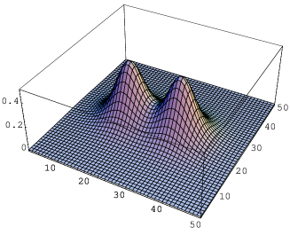
Figure 7: $B(x)$ field for $\epsilon=0.9$, and 51 orders.

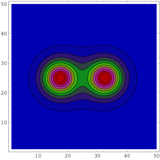
Figure 8: Contour of $B(x)$ for $\epsilon=0.9$, and 51 orders.

Focusing on the results for large areas, we emphasise that the main effect of a change in $\epsilon$ will the be to vary the separation between the vortices. Thus, with the coefficients obtained from our analysis we can actually explore the variations in shape for nearby vortices as a function of separation, a study which can have some interest (see for example Ref.Burzlaff:2000wv ). In this ($\epsilon\sim 1$) case, we can also compare with other alternative methods. In particular, in Ref. Samols:ne the two vortex solution is computed by numerical methods. The finite square size used corresponds to $\epsilon=0.91$ and the precision attained $10^{-4}$. Our formulas give a precision in the $10^{-5}-10^{-4}$ for this size, which is, at least, as good.

4 Conclusions

Let us summarise our results. We have shown how one can expand the solutions of the Bogomolny equations on a two dimensional torus in powers of $\epsilon=1-2f$, where $f$ is the average magnetic field (flux over area). The coefficients of the Fourier modes can be constructed using an iterative procedure involving convolutions. Although, no close analytical expression for the coefficients exist beyond the first non-trivial order, these coefficients can be determined up to double precision machine accuracy (15-17 significant digits), by truncating to a finite number of modes. This method can be applied to construct solutions with arbitrary flux and location of the Higgs field zeroes. We have computed the coefficients for a couple of cases ($q=1$ and $q=2$) and the results are very encouraging. The 51 order truncated expansion is estimated to describe the shape of the function within machine precision up to areas which are two and a half times the critical area. But meaningful values can be extracted also for large sizes, where due to the exponential localisation of the solution, the configurations are close to those of infinite area. In particular, these results match nicely with what is known about the unit-vortex on the plane. Turning the information around, this allows to obtain precise expectations about the behaviour of the coefficients for large order, which are satisfied by the data. No significant difference in performance is observed when studying multivortex solutions.

The solutions on the torus are relevant to depict the behaviour of the system in a situation of high vortex density. Their thermodynamics was analysed in Ref. Shah:1993us . The description in terms of Fourier modes has been used previously in other contexts, like in the study of skyrmion crystals Ref. kugler ; castillejo . It seems, however, on the basis of our results, that our method can be used successfully to study the infinite area case as well.

There are a number of possible applications and generalisations of the method to other problems or situations, some of which are currently under study. Special mention deserves the application to self-dual configurations on the four dimensional torus. In this case, there are no explicit analytic formulas for the solutions and the present method might provide good results, as an alternative to numerical methods GarciaPerez:1989gt . Actually, the first term in the expansion was obtained previously GarciaPerez:2000yt and served as initial motivation of this work.

There are other interesting problems for which the present method can be used. For example, in the study of the dynamics of vortices, specially in the low energy limit in which the geodesic approximation is valid Manton:1981mp ; Stuart:tc . The main issue here is the determination of the metric within the manifold of solutions. This metric can be extracted from the behaviour of the solution itself in the vicinity of the Higgs zeroes Samols:ne , which suggests that our method can be successfully usedin_prep . This study offers the opportunity to express and analyse the conserved quantities studied in Ref. mantonnasir within our formalism.

Finally, it is interesting to notice that the critical area case has a generalisation to Higgs-gauge systems in any Kahler manifold, in what is called the Bradlow limitBradlow:ir . From this point of view, our expansion can be viewed as a particular case of a much more general concept: an expansion in the Bradlow parameter. Although part of our technology is specific to the torus, we think that there are appropriate generalisations to other manifolds and Riemannian metrics by using a different set of basis functions. Indeed, the lowest term has already studied for the case of the two-sphereBaptista:2002kb . These generalisations are currently under study by the present authors.

Appendix A Quantum mechanical formalism

In this section we will describe the formalism in quantum mechanical terms. Here we follow the spirit, notation and formulas of Ref. Giusti:2001ta . Our goal is to characterise the space of sections of a U(1) vector bundle on the two-dimensional torus within a fixed trivialisation.

Fields satisfying the boundary conditions (5-7) make up a pre-Hilbert space ${\cal H}_{q}$ with scalar product

$$\langle\Phi|\Psi\rangle=\frac{1}{\cal A}\int_{T^{2}}dx\;\Phi^{*}(x)\Psi(x)$$ (55)

where ${\cal A}$ is the area of the torus. The integration is over the torus and because of the integrand periodicity can be performed over any fundamental cell.

Following the standard quantum mechanical procedure we will now look for a complete set of commuting operators which can serve to find a basis of the Hilbert space. One family of operators ${\mathbf{U}}_{\tilde{a}}$ is labelled by elements $\tilde{a}$ of the dual lattice $\Lambda^{*}$:

$${\mathbf{U}}_{\tilde{a}}\Psi(x)=\exp\{2\pi\imath\tilde{a}(x)\}\Psi(x)$$ (56)

where $\tilde{a}$ is a linear function of $x$ satisfying $\tilde{a}(e^{(i)})\in{\mathbf{Z}}$. Notice that we can introduce two special elements $\omega_{i}$ of $\Lambda^{*}$ associated with the form $\omega$:

$$\omega_{i}(x)=\frac{\omega(e^{(i)},x)}{q}$$ (57)

The set of these two elements is the dual basis to $\{e^{(i)}\}$. All the ${\mathbf{U}}_{\tilde{a}}$ operators are mutually commuting. They are just gauge transformations of a special kind.

In addition we will look at operators implementing translations. However, ordinary translations map out of ${\cal H}_{q}$ because the transition functions depend on $x$. It is clear on the basis of the nature of our fields that we should replace translations by appropriate parallel transporters. For that purpose we will make use of the privileged connection $A^{(0)}$ on the torus, having constant (or uniform) field strength:

$$A^{(0)}=\pi\omega(x,dx)$$ (58)

Finite translation operators ${\cal T}_{a}$ can be defined as parallel transporters along straight lines:

$$({\cal T}_{a}\Psi)=e^{-\imath\int_{\gamma}A^{(0)}}\;\Psi(x+a)=e^{-\imath\pi\omega(x,a)}\,\Psi(x+a)$$ (59)

Obviously these operators do not commute: their commutator is determined by the flux of the gauge field through the corresponding parallelogram.

Our boundary conditions can be then reformulated by saying that elements of ${\cal H}_{q}$, are those fields left invariant by the operators:

$${\cal T}_{e^{(i)}}{\mathbf{U}}_{(-qw_{i})}$$ (60)

We can then introduce the operators

$$K^{(i)}={\cal T}_{-e^{(i)}/q}\,{\mathbf{U}}_{w_{i}}$$ (61)

and re-express the boundary conditions by saying that $(K^{(i)})^{q}={\mathbf{I}}$. Furthermore the operators obey:

$$K^{(1)}K^{(2)}=\exp\{2\pi\imath/q\}\ K^{(2)}K^{(1)}$$ (62)

The operator $K^{(1)}$ generates a $Z_{q}$ group and its eigenvalues are given by $\exp\{-2\pi\imath\frac{s}{q}\}$, where $s$ is an integer modulo $q$. Thus, one can decompose ${\cal H}_{q}$ into the $q$ orthogonal subspaces of eigenvectors:

$${\cal H}_{q}=\oplus_{s=1}^{q}{\cal H}_{q,s}$$ (63)

$K^{(2)}$ maps ${\cal H}_{q,s}$ into ${\cal H}_{q,s-1}$. The translation operators ${\cal T}_{a}$ commute with $K^{(i)}$ and hence leave these subspaces invariant.

Our task of finding a complete set of operators is achieved by $K^{(1)}$ and an operator involving translations. As we will see in the study of the Bogomolny equation it is natural to select this operator to be the covariant Laplacian constructed with the constant field strength gauge potential. Up to now the choice of metric in space has played no basic role. Here, however, this operator depends on the metric. We will take the metric to be Euclidean. Within this metric the lattice vectors $e^{(i)}$ have a well defined length and scalar product. It is always possible to make a coordinate transformation to bring $e^{(1)}$ to the form $(l_{1},0)$. The other vector $e^{(2)}$ is then given by $l_{2}(\cos\varphi,\sin\varphi)$. This reduces for $\varphi=\frac{\pi}{2}$ to the special case considered in section 2.

The generators of translations along each axis are precisely the components of the covariant derivative corresponding to the $A^{(0)}$ field. We obtain

$$D^{(0)}_{i}=\partial_{i}+\pi\imath q\epsilon_{ij}x_{j}/{\cal A}$$ (64)

where $\epsilon_{ij}$ is the antisymmetric tensor with two indices($\epsilon_{12}=1$), and ${\cal A}$ is the area of the fundamental cell. These operators are anti-hermitian and satisfy the following commutation relations:

$$[D_{1}^{(0)},D_{2}^{(0)}]=-\imath f\equiv\frac{-2\pi\imath q}{{\cal A}}$$ (65)

After an appropriate rescaling this is just the Heisenberg algebra satisfied by momentum and position operators in one dimensional Quantum Mechanics. Using standard formulas one can construct operators $\mathbf{a}$, $\mathbf{a}^{\dagger}$ satisfying the commutation relations of creation-annihilation operators, and express the covariant derivatives in terms of them:

$$D_{1}^{(0)}=i\sqrt{\frac{f}{2}}(\mathbf{a}+\mathbf{a}^{\dagger})$$ (66)

$$D_{2}^{(0)}=\sqrt{\frac{f}{2}}(\mathbf{a}-\mathbf{a}^{\dagger})$$ (67)

The covariant Laplacian associated to the $A^{(0)}$ field is proportional to the Hamiltonian of a harmonic oscillator:

$$D_{i}^{(0)}D_{i}^{(0)}=-f(\mathbf{a}^{\dagger}\mathbf{a}+\frac{1}{2})$$ (68)

Thus the space of classical sections of a U(1) bundle, has identical structure as the Landau levels of the quantum system.

Finally, a basis of our space of sections is provided by the states $|n,s\rangle$ which are simultaneous eigenstates of the number operator and $K^{(1)}$, where $n$ is an arbitrary non-negative integer and $s$ an integer modulo $q$. We have the following relations

$$K^{(1)}|n,s\rangle=e^{-i\frac{2\pi s}{q}}|n,s\rangle$$ (69)

$$K^{(2)}|n,s\rangle=|n,s-1\rangle$$ (70)

$$D_{1}^{(0)}|n,s\rangle=i\sqrt{\frac{f}{2}}\,(\sqrt{n+1}|n+1,s\rangle+\sqrt{n}|n-1,s\rangle)$$ (71)

$$D_{2}^{(0)}|n,s\rangle=\sqrt{\frac{f}{2}}\,(-\sqrt{n+1}|n+1,s\rangle+\sqrt{n}|n-1,s\rangle)$$ (72)

We consider the $|n,s\rangle$ states to be orthonormal within the scalar product Eq. 55.

We will now give the explicit form of the functions $\Psi_{n,s}(x_{1},x_{2})$ corresponding to these states ($|n,s\rangle$). For that purpose notice that any function $\Psi(x_{1},x_{2})\in{\cal H}_{q}$ can be expressed as:

$$\Psi(x_{1},x_{2})=e^{-\imath\pi q\omega_{1}(x)\omega_{2}(x)}\,\sum_{p\in{\mathbf{Z}}}e^{-2\pi\imath p\omega_{2}(x)}{\cal J}_{p}(\omega_{1}(x))$$ (73)

which follows from analysing the periodicity under $e^{(1)}$. Now imposing that $\Psi$ belongs to ${\cal H}_{q,s}$, one concludes that, in the sum appearing in Eq. 73, $p$ is restricted to $p=s\bmod q$. Imposing now periodicity under $e^{(2)}$ we arrive at:

$$\Psi(x_{1},x_{2})=e^{-\imath\pi q\omega_{1}(x)\omega_{2}(x)}\,\sum_{p\in s+q{\mathbf{Z}}}e^{-2\pi\imath p\omega_{2}(x)}\,{\cal J}(q\omega_{1}(x)+p)$$ (74)

Now we look at eigenstates of the number operator. For that purpose it is interesting to look at the way in which the creation and annihilation operators act on the function ${\cal J}$ appearing in the previous formula. We have:

$$(\mathbf{a}{\cal J})(y)=\frac{1}{\sqrt{2}}(\frac{d}{dy^{\prime}}-\imath\frac{e^{i\varphi}}{\sin\varphi}y^{\prime}){\cal J}(y)$$ (75)

$$(\mathbf{a}^{\dagger}{\cal J})(y)=\frac{-1}{\sqrt{2}}(\frac{d}{dy^{\prime}}-\imath\frac{e^{-i\varphi}}{\sin\varphi}y^{\prime}){\cal J}(y)$$ (76)

where $y^{\prime}=\sqrt{\frac{2\pi l_{2}\sin\varphi}{ql_{1}}}y$.

After a standard quantum mechanical calculation we arrive at the expression of the function $\Psi_{ns}(x_{1},x_{2})$ corresponding to the state $|n,s\rangle$

$$\Psi_{ns}(x_{1},x_{2})=(\frac{2ql_{2}\sin\varphi}{l_{1}})^{1/4}\,e^{-\imath\pi q\omega_{1}(x)\omega_{2}(x)}\,\sum_{p\in s+q{\mathbf{Z}}}e^{-2\pi\imath p\omega_{2}(x)}e^{\imath\frac{e^{\imath\varphi}}{2\sin\varphi}y^{\prime 2}}H_{n}(y^{\prime})$$ (77)

where $H_{n}$ is a Hermite polynomial and $y^{\prime}=\sqrt{f}(x_{2}+\frac{pl_{2}\sin\varphi}{q})$. To reduce to the case of orthogonal $e^{(i)}$ one can fix $\varphi=\frac{\pi}{2}$, $\omega_{1}(x)=x_{2}/l_{2}$ and $\omega_{2}(x)=-x_{1}/l_{1}$.

For the special case of the vacuum state ($n=0$), we get

$$\Psi_{0s}(x_{1},x_{2})=(\frac{2ql_{2}\sin\varphi}{l_{1}})^{1/4}\,e^{-\imath\pi q\omega_{1}(x)\omega_{2}(x)}\,e^{\imath\pi\tau\omega_{1}^{2}}\,\vartheta\left[\begin{array}[]{c}s/q\\ 0\end{array}\right](z,\tau)$$ (78)

where $\vartheta\left[\begin{array}[]{c}s/q\\ 0\end{array}\right](z,\tau)$ is a theta function with rational characteristics with arguments:

$$z=\pi(\tau\omega_{1}-q\omega_{2})$$ (79)

$$\tau=e^{\imath\varphi}q\frac{l_{2}}{l_{1}}$$ (80)

Now we need to deduce the action of the translation operator ${\cal T}(a)$ on these states. The translation operator is defined as ${\cal T}(a)=\exp\{a_{1}D_{1}^{(0)}+a_{2}D_{2}^{(0)}\}=\exp\{-(z(a)\mathbf{a}-z^{*}\mathbf{a}^{\dagger})\}$. Now we can compute the matrix elements

$$\langle m,s^{\prime}|{\cal T}(a)|n,s\rangle=\delta_{ss^{\prime}}\,e^{i\beta(n-m)}(-1)^{(M+n)}\times$$ (81)

$$\,e^{-\frac{|z|^{2}}{2}}|z|^{|m-n|}\sum_{j=0}^{M}(-1)^{j}\frac{\sqrt{n!m!}\,|z|^{2j}}{j!(M-j)!(j+|m-n|)!}$$

where $M=\min{(m,n)}$ and

$$z(a)=-i\sqrt{\frac{f}{2}}(a_{1}-ia_{2})\equiv|z|e^{i\beta}$$ (82)

We can also compute the matrix elements of the operators ${\mathbf{U}}_{\tilde{a}}$. Expanding $\tilde{a}$ in the dual basis of $\Lambda^{*}$ we can write $\tilde{a}(x)=-k_{1}\omega_{2}(x)+k_{2}\omega_{1}(x)$. We will then denote ${\mathbf{U}}_{\tilde{a}}\equiv U(k_{1},k_{2})$. This operator can be expressed in terms of $K^{(i)}$ and translations as follows:

$$U(k_{1},k_{2})=e^{-i\pi\frac{k_{1}k_{2}}{q}}\,(K^{(2)})^{-k_{1}}(K^{(1)})^{k_{2}}{\cal T}(a(k_{1},k_{2}))$$ (83)

From here we can compute the matrix elements:

$$\langle m,s^{\prime}|U(k_{1},k_{2})|n,s\rangle=\delta_{s^{\prime}\,s+k_{1}}e^{2\pi i\frac{sk_{2}}{q}}\,e^{-i\pi\frac{k_{1}k_{2}}{q}}\,e^{i\alpha(n-m)}(-1)^{(M+n)}\times$$ (84)

$$\,e^{-\frac{\tilde{\xi}}{2}}\tilde{\xi}^{|m-n|/2}\sum_{j=0}^{M}(-1)^{j}\frac{\sqrt{n!m!}\,\tilde{\xi}^{j}}{j!(M-j)!(j+|m-n|)!}$$

where $\alpha$ and $\tilde{\xi}$ can be obtained from the complex number

$$\kappa=-\imath\sqrt{\frac{f}{2}}(l_{1}k_{2}-l_{2}k_{1}e^{i\varphi})/q=\sqrt{\tilde{\xi}}\,e^{\imath\alpha}$$ (85)

and $\tilde{\xi}$ is the generalisation of $\xi$ defined in Eq. 22 to the case of non-orthogonal $e^{(i)}$:

$$\tilde{\xi}=|\kappa|^{2}=\frac{\pi}{q\sin\varphi}(k_{1}^{2}\frac{l_{2}}{l_{1}}+k_{2}^{2}\frac{l_{1}}{l_{2}}-2k_{1}k_{2}\cos\varphi)$$ (86)

A.1 The Bogomolny equations

We can now reformulate the Bogomolny equations in this formalism. We can write the Higgs field as $\phi=\epsilon\psi$, where $\psi$ is a normalised element of ${\cal H}_{q}$. It can be decomposed in our basis

$$\psi=\sum_{n=0}^{\infty}c(n,s)\,|n,s\rangle$$ (87)

where the sum of the modulus square of the coefficients $c(n,s)$ equals unity. Similarly the function $h$ appearing in Section 2 is expressed in terms of a generalised Fourier decomposition

$$h(x_{1},x_{2})=\sum_{k_{1}k_{2}}\,h_{k_{1}k_{2}}e^{2\pi i(-k_{1}\omega_{2}(x)+k_{2}\omega_{1}(x))}\,$$ (88)

The first Bogomolny equation can then be expressed as follows:

$$\mathbf{a}\psi=i\frac{1}{\sqrt{2f}}\left((\partial_{1}+i\partial_{2})h\right)\psi$$ (89)

Hence, using the decompositions of $h$ and $\psi$ and the matrix elements deduced in this Section, we can re-express the Bogomolny equations as follows:

$$(1-\epsilon)|\kappa|^{2}h_{k_{1}k_{2}}=\frac{\epsilon}{2}\sum_{m,s^{\prime},n,s}\,c^{*}(m,s^{\prime})\,c(n,s)\,\langle m,s^{\prime}|U(-k_{1},-k_{2})|n,s\rangle$$ (90)

$$\sqrt{n+1}\,c(n+1,s^{\prime})=-\sum_{k_{1}k_{2}}\,\kappa^{*}h_{k_{1}k_{2}}\,\sum_{p,s}\,c(p,s)\,\langle n,s^{\prime}|U(k_{1},k_{2})|p,s\rangle$$ (91)

where $\kappa=\imath\sqrt{\frac{f}{2}}(k_{1}l_{2}e^{-\imath\varphi}-k_{2}l_{1})/q$. The volume dependence of these equations is explicit (contained in the dependence on $\epsilon$). Our method consists then in expanding the unknown coefficients in powers of $\epsilon$:

$$c(p,s)=\sum_{k=0}^{\infty}c^{(k)}(p,s)\,\epsilon^{k}$$ (92)

$$h_{k_{1}k_{2}}=\sum_{k=1}^{\infty}h^{(k)}_{k_{1}k_{2}}\,\epsilon^{k}$$ (93)

and solving the equations order by order.

Let us compute the leading terms for the $q=1$ case. To lowest non-trivial order we have

$$c^{(0)}(n)=\delta_{n0}$$ (94)

and $h^{(0)}_{k_{1}k_{2}}=0$. Then, plugging this value into the first Bogomolny equation we get:

$$h^{(1)}_{k_{1}k_{2}}=\frac{1}{\tilde{\xi}}\langle 0|U(-k_{1}-k_{2})|0\rangle=\frac{(-1)^{k_{1}k_{2}}}{2\tilde{\xi}}\,e^{-\tilde{\xi}/2}$$ (95)

The following order obtains from the other equation

$$c^{(1)}(n)=-\frac{1}{\sqrt{n}}\sum_{k_{1}k_{2}}\,\kappa^{*}h^{(1)}(k_{1},k_{2})\,\langle n-1|U(k_{1},k_{2})|0\rangle=-\frac{1}{2\sqrt{n!}}\sum_{k_{1}k_{2}}\,\frac{(\kappa^{*})^{n}}{\tilde{\xi}}\,e^{-\tilde{\xi}}$$ (96)

This is real and vanishes for odd $n$.

One can then continue to iterate Eqs. 90–91 to higher orders in $\epsilon$. To evaluate the expressions one has to restrict to a finite number of elements on the basis. Now, in addition to the cut in Fourier modes $n_{\mbox{\tiny max}}$, one has to cut in the spectrum of the number operator $n\leq n_{\mbox{\tiny part}}$. As the order $k$ grows both $n_{\mbox{\tiny max}}$ and $n_{\mbox{\tiny part}}$ should grow to keep the numbers within machine precision. We have developed an independent Fortran90 program to evaluate the $c^{(k)}(n)$, $h^{(k)}(n_{1},n_{2})$ using this procedure. With this program we have reproduced, within machine precision, the coefficients in the expansion of the low lying modes $n_{i}$ up to 30th order in the expansion for the $q=1$ case. This serves as a check that there are no unexpected bugs in the determination of the coefficients. Increasing the order one starts noticing sizable errors associated to the cut in $n_{\mbox{\tiny part}}$. Unfortunately, increasing this number is not only limited by computer resources, but also by numerical instabilities. For example the computation of the matrix elements $\langle n,s^{\prime}|U(k_{1},k_{2})|p,s\rangle$ becomes unstable for large $k_{i}$, $n$ and $p$. This is due to wild cancellations of large numbers appearing in their definition. Actually, the problem already appears at lower orders. In our calculation to order 30, we had to tabulate these matrix elements and compute them independently with a C code and the GNU Multiple Precision Arithmetic Library (GMP) which allows arbitrary precision floating point operations. The values of the matrix elements were computed up to $n_{\mbox{\tiny part}}=150$ and performing intermediate calculations with $300$ significant decimal digits. In summary, it turns out that this method is less efficient than the one explained in section 2. Nevertheless, apart from serving as a check of the results, we found interesting to explore this quantum mechanical procedure, since it seems directly generalisable to the construction of self-dual configurations in the four-dimensional torus GarciaPerez:2000yt , and all the main intermediate objects (as $\langle n,s^{\prime}|U(k_{1},k_{2})|p,s\rangle$) appear there as well. This is currently under study.

- (1) A. Vilenkin and E. P. S. Shellard “Cosmic Strings and Other Topological Defects,” Cambridge University Press, (1994)
- (2) A. A. Abrikosov, Sov. Phys. JETP 5, 1174 (1957) [Zh. Eksp. Teor. Fiz. 32, 1442 (1957)].
- (3) H.B. Nielsen and P. Olesen. Nuclear Physics, B61:45–61, 1973.
- (4) L. Kramer, Phys. Lett. 23, 619 (1966)
- (5) E. Müller Hartman, Phys. Lett. 23, 521 (1966)
- (6) E. B. Bogomolny, Sov. J. Nucl. Phys. 24, 449 (1976) [Yad. Fiz. 24, 861 (1976)].
- (7) Clifford Henry Taubes. Comm. Math. Phys., 75:207–227, 1980.
- (8) Clifford Henry Taubes. Commun. Math. Phys., 72:277, 1980.
- (9) H. J. de Vega and F. A. Schaposnik. Phys. Rev., D14:1100–1106, 1976.
- (10) E. J. Weinberg, Phys. Rev. D 19, 3008 (1979).
- (11) L. Jacobs and C. Rebbi. Phys. Rev., B19:4486–4494, 1979.
- (12) H. Arodz and L. Hadasz. Phys. Rev., D54:4004–4012, 1996.; J. Karkowski and Z. Swierczynski. Acta Phys. Polon., B30:73–87, 1999.; J. Karkowski and Z. Swierczynski. Acta Phys. Polon., B31:601–615, 2000.
- (13) M. Garcia Perez, A. González-Arroyo and C. Pena, JHEP 0009, 033 (2000) [arXiv:hep-th/0007113].
- (14) A. González-Arroyo. Yang-Mills fields on the 4-dimensional Torus. Part I: Classical Theory, Proceedings of the Peñiscola 1997 advanced school on non-perturbative quantum field physics. World Scientific, 1998.
- (15) G. N. Watson and E. T. Whittaker. A course on modern analysis. Cambridge University Press, 1969.
- (16) P. A. Shah and N. S. Manton, J. Math. Phys. 35, 1171 (1994) [arXiv:hep-th/9307165].
- (17) S. M. Nasir, Phys. Lett. 419B, 253 (1998).
- (18) N. S. Manton and S. M. Nasir, Commun. Math. Phys. 199, 591 (1999).
- (19) D. Tong, JHEP 0207, 013 (2002) [arXiv:hep-th/0204186].
- (20) J. Burzlaff and E. Kellegher, J. Math. Phys. 42, 182 (2001) [arXiv:hep-th/0007244].
- (21) T. M. Samols, Commun. Math. Phys. 145, 149 (1992).
- (22) M. Kugler and S. Shtrikman Phys. Lett., B 208:491 (1988).
- (23) L. Castillejo, P. S. J. Jones, A. D. Jackson, J. J. M. Verbaarschot and A. Jackson, Nuc. Phys. A501, (1989).
- (24) M. Garcia Perez, A. González-Arroyo and B. Soderberg, Phys. Lett. B 235, 117 (1990).; M. Garcia Perez and A. Gonzalez-Arroyo, J. Phys. A 26, 2667 (1993) [arXiv:hep-lat/9206016].
- (25) N. S. Manton, Phys. Lett. B 110, 54 (1982).
- (26) D. Stuart, Commun. Math. Phys. 166, 149 (1994).
- (27) A. González-Arroyo and A. Ramos, In preparation.
- (28) N. S. Manton and S. M. Nasir, Nonlinearity 12, 851-865 (1999) [arXiv:hep-th/9809071].
- (29) S. B. Bradlow, Commun. Math. Phys. 135, 1 (1990).
- (30) J. M. Baptista and N. S. Manton, J. Math. Phys. 44, 3495 (2003) [arXiv:hep-th/0208001].
- (31) L. Giusti, A. González-Arroyo, C. Hoelbling, H. Neuberger and C. Rebbi, Phys. Rev. D 65, 074506 (2002) [arXiv:hep-lat/0112017].